1. Introduction
Natural convection in fluid layers encompasses a broad class of instability mechanisms, ranging from the canonical Rayleigh–Bénard problem – driven exclusively by boundary thermal forcing – to systems dominated by internal heat generation (Lappa Reference Lappa2009; Goluskin Reference Goluskin2016). An intermediate configuration that exhibits characteristics of both boundary-driven and internally heated flows is that of natural convection driven by the absorption of overhead irradiation (Lei & Patterson Reference Lei and Patterson2002; Amber & O’Donovan Reference Amber and O’Donovan2018). In this setting, radiation is partially absorbed within the fluid, establishing a vertical temperature gradient that tends to stabilise the fluid layer. The remaining energy reaches and heats the bottom boundary, producing an upward heat flux that warms and destabilises the fluid. A recurring simplification in these works, however, is the assumption of an adiabatic top boundary – an idealisation that neglects surface cooling, which is often significant in realistic environments. In practice, the interplay between radiation absorption and surface cooling governs convective processes across a wide spectrum of natural and engineered systems. In the atmosphere, for instance, greenhouse gases modulate global circulation through the combined effects of solar absorption and longwave emission to space (Manabe Reference Manabe2023). In the oceans, penetrating radiation and surface cooling act together to regulate vertical mixing and large-scale thermohaline circulation (Groeskamp & Iudicone Reference Groeskamp and Iudicone2018). Engineering applications – including solar ponds, direct absorption solar collectors and CSPonD receivers – also exhibit convective dynamics shaped by this coupled physics, where absorbed radiation and surface thermal losses collectively dictate flow stability and thermal efficiency (Raj & Subudhi Reference Raj and Subudhi2018; Tetreault-Friend et al. Reference Tetreault-Friend, Diago, Cooper, Gray and Slocum2018; Calvet et al. Reference Calvet2021; Saxena et al. Reference Saxena, Cuce, Singh, Cuce, Gupta, Suryavanshi, Farrokhi and El-Sebaii2022). A fundamental understanding of this coupled mechanism is therefore essential for accurately predicting convective behaviours in geophysical contexts and for optimising the performance of energy-related systems.
Convection onset in the system, illustrated in figure 1, arises from the competition between two destabilising forcings – surface cooling and bottom heating – a mechanism that falls within the class of boundary-layer-driven Rayleigh modes (Farrow & Patterson Reference Farrow and Patterson1993; Gershuni et al. Reference Gershuni, Lyubimov, Lyubimova and Roux1994; Dittko, Kirkpatrick & Armfield Reference Dittko, Kirkpatrick and Armfield2013). This destabilisation disrupts the stable temperature stratification established by volumetric radiation absorption following the Beer–Lambert law (Lepot, Aumaître & Gallet Reference Lepot, Aumaître and Gallet2018; Bouillaut et al. Reference Bouillaut, Lepot, Aumaître and Gallet2019; Kazemi et al. Reference Kazemi, Ostilla-Mónico and Goluskin2022). Thus, the system constitutes a canonical form of penetrative convection, in which motions generated in unstable regions intrude into adjacent stably stratified zones (Arnone et al. Reference Arnone, Cantini, Capone and Carnevale2023). Specifically, the system may evolve into either a single well-mixed layer or a triple-layer structure (Zhou et al. Reference Zhou, Yang, You, Liu, Sun and Li2025). In the triple-layer regime, a stably stratified interlayer resulting from volumetric radiation absorption is sandwiched between two unstably mixed layers generated by bottom heating and surface cooling, respectively. This intricate layering gives rise to a spectrum of stability behaviours – including the near-complete suppression of convection under certain conditions (Xue, Zhang & Ni Reference Xue, Zhang and Ni2024). The interplay among volumetric radiation heating, surface cooling and bottom heating leads to a dynamic equilibrium with strongly time-dependent stability characteristics. Consequently, the stability of the system is inherently transient, requiring time-dependent analysis to accurately capture the subtle transitions between convective suppression and onset.
A fundamental problem in convective onset analysis is the determination of the critical Rayleigh number
 $\textit{Ra}_c$
, which marks the transition from a quiescent, conductive state to convective motion. Over the past century, linear stability analysis (LSA) has been widely employed to investigate the onset of hydrodynamic instability in fluid flows (Rayleigh Reference Rayleigh1916). A standard methodology for determining
 $\textit{Ra}_c$
is grounded in the classical normal mode approach (Mahajan Reference Mahajan2024), where the assumption of marginal stability transforms the stability problem into an eigenvalue problem (Arnone et al. Reference Arnone, Cantini, Capone and Carnevale2023; Ding & Ouyang Reference Ding and Ouyang2023). For certain systems, analytical expressions for
 $\textit{Ra}_c$
can be obtained through specialised techniques such as asymptotic expansion (Goluskin Reference Goluskin2015; Praveena, Babu & Bixapathi Reference Praveena, Babu and Bixapathi2025).
Schematic of the convection system.

Another essential problem concerns the prediction of the critical time
 $t_c$
for flow onset, which arises when the Rayleigh number
 $\textit{Ra}$
exceeds the critical value
 $\textit{Ra}_c$
. To address this, several time-dependent LSA approaches have been developed, including the frozen-time model, propagation theory and amplification theory. The frozen-time model treats the temporally evolving base flow as a sequence of stationary states by analysing stability at discrete, frozen instants (Gresho & Sani Reference Gresho and Sani1971; Doumenc et al. Reference Doumenc, Boeck, Guerrier and Rossi2010). This approach predicts the onset time of growing instabilities, a theoretical threshold marking the initial growth of infinitesimal perturbations. A notable feature of this prediction is its independence of the Prandtl number
 $\textit{Pr}$
(Hattori, Patterson & Lei Reference Hattori, Patterson and Lei2015b
). Nevertheless, in many experimental and natural settings, the moment of greater practical importance is the detection time of manifest convection, which exhibits a clear dependence on
 $\textit{Pr}$
(Choi et al. Reference Choi, Park, Kim, Lee, Kim and Davis2004; Tilton Reference Tilton2018). Propagation theory offers an alternative framework by rescaling the governing equations with the thermal penetration depth, enabling a self-similar analysis of disturbance growth in developing thermal boundary layers (TBLs) under transient conditions (Choi et al. Reference Choi, Kang, Kim and Hwang1998; Saravanan & Vigneshwaran Reference Saravanan and Vigneshwaran2025). A limitation of this approach, however, is its reliance on specific mathematical transformations and a particular form of the conductive temperature profile, which restricts its applicability to the present configuration. Amplification theory, in contrast, directly examines the spatiotemporal evolution of transient perturbations, assessing system instability by computing the maximum amplification factor of a perturbation over a prescribed time interval (Foster Reference Foster1965; Sabet, Hassanzadeh & Abedi Reference Sabet, Hassanzadeh and Abedi2018; Tilton Reference Tilton2018). The primary challenge with this method is the absence of a universally accepted, physically motivated criterion for instability; assessments are therefore inherently empirical and require cross-validation against other methods (Jaupart & Parsons Reference Jaupart and Parsons1985; Rapaka et al. Reference Rapaka, Chen, Pawar, Stauffer and Zhang2008; Doumenc et al. Reference Doumenc, Boeck, Guerrier and Rossi2010).
A conceptually simpler alternative to the aforementioned LSA frameworks is the local
 $\textit{Ra}$
criterion (Bejan Reference Bejan2013). Defined in terms of the instantaneous TBL thickness, the local
 $\textit{Ra}$
provides a physically intuitive predictor for the onset of instability: convection is expected to emerge once this local value exceeds a critical threshold. This approach has been employed in previous studies to estimate the onset time of convective instability (Tan & Thorpe Reference Tan and Thorpe1996; Hattori et al. Reference Hattori, Patterson and Lei2015c
).
In light of the above-mentioned discussion, the goal of the present work is to determine
 $\textit{Ra}_c$
and
 $t_c$
for the onset of transient natural convection induced by radiation absorption and surface cooling. To this end, we employ LSA to investigate the temporal evolution of stability. The transition of instability modes, such as the global mode relevant to the single-layer structure and the local mode specific to the triple-layer structure, is expected to be identified. For the local instability mode, a local
 $\textit{Ra}$
model is developed to predict the critical threshold, thereby connecting the system’s behaviour to the classical Rayleigh–Bénard instability framework. Scaling laws for
 $t_c$
are derived and the amplification theory is adopted to clear the dependence of
 $t_c$
on all key governing parameters. The entire theoretical framework is then rigorously validated against direct numerical simulations (DNSs), establishing a robust predictive tool for convective onset in this class of systems.
The remainder of this paper is organised as follows. The mathematical formulation of the convection system induced by radiation absorption and surface cooling is presented in § 2. In § 3.1, two distinct linear stability approaches are employed: the marginal stability assumption to predict
 $\textit{Ra}_c$
, and the amplification theory to determine both
 $\textit{Ra}_c$
and
 $t_c$
. The local
 $\textit{Ra}$
model is developed in § 3.2, followed by the derivation of scaling laws for
 $t_c$
via scaling analysis in § 3.3. All theoretical predictions are validated in § 4 through DNS. Finally, concluding remarks are drawn in § 5.
2. Problem description and mathematical formulation
We consider a two-dimensional semitransparent Newtonian fluid layer of depth
 $H^*$
, bounded by a rigid bottom and a free top surface, subject to internal heating from uniform collimated irradiation with incident flux
 $I_0$
(see figure 1). The fluid is initially stationary and isothermal. The radiative intensity decays exponentially along the penetration path according to the Beer–Lambert law, giving rise to a nonlinear volumetric heat source (Hattori et al. Reference Hattori, Patterson and Lei2015a
),
 \begin{equation} S = I_0 \eta \exp (\eta z^*), \end{equation}
where
 $\eta$
is the bulk absorption coefficient of the fluid.
The rigid black bottom wall absorbs residual radiation and re-emits it as a heating flux,
 \begin{equation} u^*=w^*=0,\quad -\lambda \frac {\partial T^*}{\partial z^*} = I_0\exp (-\eta H^*),\quad \text{at} \quad z^*=-H^*, \end{equation}
where
 $u^*$
and
 $w^*$
represent the velocity components in the
 $x^*$
and
 $z^*$
directions respectively,
 $T^*$
the temperature, and
 $\lambda$
the thermal conductivity of fluid. The free top surface loses heat through a prescribed flux
 $q_0$
,
 \begin{equation} \frac {\partial u^*}{\partial z^*}=w^*=0, \quad -\lambda \frac {\partial T^*}{\partial z^*} = q_0, \quad \text{at} \quad z^*=0. \end{equation}
In general,
 $q_0$
is not equal to the radiative input
 $I_0$
; for example, in a solar collector,
 $q_0 \lt I_0$
must be maintained, whereas in a lake, a balance between
 $q_0$
and
 $I_0$
is required only over long time scales (e.g. a day or longer). Here, we assume
 $q_0$
to be constant. This assumption is justified because the constant-flux top boundary condition is appropriate for systems in which surface temperature fluctuations are small relative to the system-environment temperature difference, as supported by experimental studies (Li Reference Li2018; Pushtaev et al. Reference Pushtaev, Vinnichenko, Plaksina and Uvarov2021). In particular, in the present study, the onset of convection occurs over a short time scale, during which variations in surface temperature are negligible. Additionally, periodic boundary conditions are imposed in the horizontal direction.
The physical properties of fluid, including density
 $\rho$
, thermal diffusivity
 $a$
, thermal expansion coefficient
 $\beta$
, specific heat capacity
 $C_{\!p}$
, kinematic viscosity
 $\nu$
and thermal conductivity
 $\lambda$
, are all assumed constant. The gravitational acceleration is denoted by
 $g$
. Under the Boussinesq approximation and accounting for the radiative heating, the governing equations are
 \begin{equation} \frac {\partial u^*}{\partial x^*}+\frac {\partial w^*}{\partial z^*}=0, \end{equation}
 \begin{equation} \frac {\partial u^*}{\partial t^*}+u^*\frac {\partial u^*}{\partial x^*}+w^*\frac {\partial u^*}{\partial z^*}=-\frac {1}{\rho }\frac {\partial p^*}{\partial x^*}+\nu {\nabla} ^2 u^*, \end{equation}
 \begin{equation} \frac {\partial w^*}{\partial t^*}+u^*\frac {\partial w^*}{\partial x^*}+w^*\frac {\partial w^*}{\partial z^*}=-\frac {1}{\rho }\frac {\partial p^*}{\partial z^*}+\nu {\nabla} ^2 w^*+\beta g \big(T^*-T_{\textit{ref}}^*\big), \end{equation}
 \begin{equation} \frac {\partial T^*}{\partial t^*}+u^*\frac {\partial T^*}{\partial x^*}+w^*\frac {\partial T^*}{\partial z^*}=a{\nabla} ^2T^*+\frac {I_0 \eta }{\rho C_{\!p}}\exp (\eta z^*), \end{equation}
where
 $t^*$
represents the time,
 $p^*$
the pressure and
 $T_{\textit{ref}}^*$
the reference temperature. Here, we adopt the spatially averaged temperature
 $\langle T^* \rangle$
of the convection system as the reference temperature. Owing to the imbalance between the heat input
 $I_0$
and the surface heat loss
 $q_0$
,
 $\langle T^* \rangle$
increases linearly with time:
 \begin{equation} \langle T^* \rangle = T_0^* + \frac {I_0-q_0}{\rho C_{\!p} H^*}t^*, \end{equation}
where
 $T_0^*$
is the initial temperature.
We introduce the following dimensionless variables:
 \begin{equation} \left \{ \begin{array}{ll}\!\! \left (x, z\right ) = \eta \left (x^*, z^*\right )\!, \\[5pt] \!\! \left (u, w\right ) = \frac {1}{a\eta }\left (u^*, w^*\right )\!, \\[5pt] \!\! t = a\eta ^2 t^*, \\[5pt] \!\! p = \frac {C_{\!p} a \eta ^2}{g \beta I_0}p^*, \\[13pt] \!\! T = \frac {\rho C_{\!p} a \eta }{I_0} \big (T^* - T_{\textit{ref}}^* \big ). \end{array} \right . \end{equation}
Substituting (2.9) into (2.4)–(2.7) yields the dimensionless governing equations
 \begin{equation} \frac {\partial u}{\partial x}+\frac {\partial w}{\partial z}=0, \end{equation}
 \begin{equation} \frac {\partial u}{\partial t}+u\frac {\partial u}{\partial x}+w\frac {\partial u}{\partial z}=-\textit{RaPr}\frac {\partial p}{\partial x}+\textit{Pr}{\nabla} ^2 u, \end{equation}
 \begin{equation} \frac {\partial w}{\partial t}+u\frac {\partial w}{\partial x}+w\frac {\partial w}{\partial z}=-\textit{RaPr}\frac {\partial p}{\partial z}+\textit{Pr}{\nabla} ^2w+\textit{RaPrT}, \end{equation}
 \begin{equation} \frac {\partial T}{\partial t}+u\frac {\partial T}{\partial x}+w\frac {\partial T}{\partial z}={\nabla} ^2T+\exp (z)-\frac {1-\phi }{H}. \end{equation}
The boundary conditions become
 \begin{equation} u=w=0,\quad \frac {\partial T}{\partial z} = -\exp (-H),\quad \mbox{at} \quad z=-H, \end{equation}
 \begin{equation} \frac {\partial u}{\partial z}=w=0, \quad \frac {\partial T}{\partial z} = -\phi , \quad \mbox{at} \quad z=0, \end{equation}
and the initial condition is
 \begin{equation} u=w=0, \quad T = 0, \quad \mbox{at} \quad t=0. \end{equation}
The control parameters appearing in the earlier formulation are the Rayleigh number
 $\textit{Ra}$
, the Prandtl number
 $\textit{Pr}$
, the cooling parameter
 $\phi$
and the dimensionless depth
 $H$
:
 \begin{equation} \textit{Ra}=\frac {\beta g I_0}{\rho C_{p} \nu a^2 \eta ^4},\quad \textit{Pr}=\frac {\nu }{a},\quad \phi =\frac {q_0}{I_0},\quad H=\eta H^*. \end{equation}
The cooling parameter
 $\phi$
quantifies the intensity of surface heat loss and can take any positive value in practical systems. In the context of solar collectors,
 $1-\phi$
represents the heat collecting efficiency and the condition
 $\phi \lt 1$
must be satisfied. The dimensionless depth
 $H$
measures the optical thickness of the fluid layer. For a given fluid, a larger
 $H$
corresponds to a greater physical depth. For different fluids at the same geometric depth, a larger
 $H$
indicates a higher absorption coefficient. In either case, as evident from the bottom boundary condition (2.14), a larger
 $H$
implies weaker bottom heating.
We adopt the spatially averaged temperature
 $\langle T^* \rangle$
as the reference in (2.9), so that the dimensionless temperature
 $T$
represents the deviation from the instantaneous mean temperature of the system. By construction, the spatial average
 $\langle T \rangle$
remains zero at all times (Mique et al. Reference Miquel, Bouillaut, Aumaître and Gallet2020). An alternative choice is to reference the initial temperature, as done by Lei & Patterson (Reference Lei and Patterson2002), in which case, the dimensionless temperature measures the departure from the initial state and its spatial average increases linearly with time. The constant in the source term in (2.13) would then vanish. Nevertheless, the two formulations are physically equivalent, as they describe the same convection system and convection is driven by temperature differences rather than by absolute temperature itself.
3. Theoretical analysis
3.1. Linear stability analysis
Before the onset of flow, the fluid remains static and the energy equation (2.13) is reduced to a one-dimensional differential equation of heat conduction, which has been solved through the Laplace transform by Zhou et al. (Reference Zhou, Yang, You, Liu, Sun and Li2025) as
 \begin{eqnarray} T_{\textit{st}}(t,z) &=& -\exp \left (z\right )+\left (1-\phi \right )\left (\frac {z^2}{2H}+z+\frac {H}{3}\right ) + \frac {1}{H}\left [1-\exp \left (-H\right )\right ] \nonumber \\ &&-\frac {2}{H}\sum _{n = 1}^{\infty }\left \{\left [\frac {1-\phi }{\left (n\pi /H\right )^2}-\frac {1-\left (-1\right )^n \exp \left (-H\right )}{1+\left (n\pi /H\right )^2}\right ]\right . \nonumber \\ &&\left .\times \exp \left [-\left (\frac {n\pi }{H}\right )^2t\right ]\cos \left (\frac {n\pi }{H}z\right )\right \}\!, \end{eqnarray}
where the subscript
 $(\boldsymbol{\cdot })_{\textit{st}}$
denotes the static state.
The series (3.1) converges very slowly at early times (
 $t \rightarrow 0$
). For practical calculations at small times (
 $t \leqslant 0.1$
), we use an asymptotic solution that retains only the leading-order contributions,
 \begin{eqnarray} T_{\textit{st}} (t,z) & \thickapprox & 2 \left (1-\phi \right )\sqrt {\frac {t}{\pi }}\exp \left (-\frac {z^2}{4t}\right )+\left (1-\phi \right )z\boldsymbol{\cdot }\operatorname {erfc}\left (-\frac {z}{2\sqrt {t}}\right ) \nonumber \\ &&-\frac {1}{2}\exp \left (z+t\right )\boldsymbol{\cdot }\operatorname {erfc}\left (-\frac {z}{2\sqrt {t}}-\sqrt {t}\right )+\frac {1}{2}\exp \left (-z+t\right )\boldsymbol{\cdot }\operatorname {erfc}\left (-\frac {z}{2\sqrt {t}} + \sqrt {t}\right ) \nonumber \\ &&+\frac {\exp \left (-H\right )}{2}\exp \left [-\left (z+H\right )+t\right ]\boldsymbol{\cdot }\operatorname {erfc}\left (\frac {z+H}{2\sqrt {t}}-\sqrt {t}\right ) \nonumber \\ &&-\frac {\exp \left (-H\right )}{2}\exp \left [\left (z+H\right )+t\right ]\boldsymbol{\cdot }\operatorname {erfc}\left (\frac {z+H}{2\sqrt {t}}+\sqrt {t}\right ) \nonumber \\ &&-\exp \left (z\right )\left [1 - \exp \left (t\right )\right ] -\frac {1-\phi }{H}t. \end{eqnarray}
In the LSA, the flow variables are decomposed into a static state and infinitesimal perturbations:
 \begin{equation} \left (u,w,p,T\right ) = \left (u_{\textit{st}},w_{\textit{st}},p_{\textit{st}},T_{\textit{st}}\right )+\epsilon \big (\tilde {u},\tilde {w},\tilde {p},\tilde {T}\big ), \end{equation}
where the tilde
 $\tilde {(\boldsymbol{\cdot })}$
denotes the perturbations and
 $\epsilon \ll 1$
is the perturbation amplitude. In the present system, the base flow is motionless, so the temperature field is purely conductive, given by (3.1) and (3.2). Substituting the decomposition (3.3) into the governing equations (2.10)–(2.13), linearising by neglecting terms of
 $O(\epsilon ^2)$
and eliminating the pressure perturbation yields the linear system:
 \begin{equation} \left \{ \begin{array}{ll} \!\! \left (\frac {\partial }{\partial t}-\textit{Pr}{\nabla} ^2\right ){\nabla} ^2 \tilde {w} = \textit{RaPr}\frac {\partial ^2 \tilde {T}}{\partial x^2}, \\[11pt] \!\! \frac {\partial \tilde {T}}{\partial t}+\tilde {w}\frac {\partial T_{\textit{st}}}{\partial z}={\nabla} ^2\tilde {T}. \end{array} \right . \end{equation}
Owing to the horizontal periodicity of the domain, the perturbations are expressed in the form of normal modes with horizontal wavenumber
 $k$
(Christopher, Le Bars & Smith Reference Christopher, Le Bars and Smith2023):
 \begin{equation} \left \{ \begin{array}{ll}\!\! \tilde {w}(x,z,t) = \hat {w}(z,t)\exp (-i k x), \\ \!\! \tilde {T}(x,z,t) = \hat {T}(z,t)\exp (-i k x). \end{array} \right . \end{equation}
Substituting the normal mode expansion (3.5) into the linearised system (3.4) leads to the following governing equations for the perturbation amplitudes:
 \begin{equation} \left \{ \begin{array}{ll}\!\! \left (\frac {\partial ^2}{\partial z^2}-k^2\right )\frac {\partial \hat {w}}{\partial t} = \textit{Pr}\!\left (\frac {\partial ^2}{\partial z^2}-k^2\right )^2\hat {w}-\textit{RaPr}k^2\hat {T}, \\[11pt] \!\! \frac {\partial \hat {T}}{\partial t}=-\frac {\partial T_{\textit{st}}}{\partial z}\hat {w}+\left (\frac {\partial ^2}{\partial z^2}-k^2\right )\hat {T}. \end{array} \right . \end{equation}
The corresponding boundary conditions for (3.6) are given by
 \begin{equation} \left \{ \begin{array}{ll}\!\! \hat {w}=\frac {\partial \hat {w}}{\partial z}=\frac {\partial \hat {T}}{\partial z}=0, & \mbox{at} \quad z=-H, \\[9pt] \!\! \hat {w}=\frac {\partial ^2 \hat {w}}{\partial z^2}=\frac {\partial \hat {T}}{\partial z}=0, & \mbox{at} \quad z=0. \end{array} \right . \end{equation}
3.1.1. Marginal stability assumption
The assumption of marginal stability implies that the temporal derivative terms in (3.6) can be eliminated. Under this assumption,
 $\textit{Pr}$
no longer appears in the governing equations, while the time dependence is retained solely through the static temperature profile
 $T_{\textit{st}}$
. The resulting eigenproblem is given by
 \begin{equation} \left \{ \begin{array}{ll}\!\! \textit{Ra} k^2\hat {T} = \left (\frac {\partial ^2}{\partial z^2}-k^2\right )^2\hat {w}, \\[7pt] \!\! 0 = \left (\frac {\partial ^2}{\partial z^2}-k^2\right )\hat {T}-\frac {\partial T_{\textit{st}}}{\partial z}\hat {w}. \end{array} \right . \end{equation}
For given
 $H$
,
 $\phi$
and
 $t$
, the flow becomes unstable when
 $\textit{Ra}$
exceeds a critical value
 $\textit{Ra}_c$
, defined as the smallest positive eigenvalue of the eigenproblem (3.8) (Farrow & Patterson Reference Farrow and Patterson1993):
 \begin{equation} \textit{Ra}_c(H,\phi ,t) = \underset {\substack {k\neq 0 \\ \textit{Ra}\gt 0}}{\min } \left \{\textit{Ra} \big (k^2,H,\phi ,t\big )\right \}\!. \end{equation}
We note that for a large
 $H$
, the minimum eigenvalue of (3.8) may be negative. It is therefore essential to define
 $\textit{Ra}_c$
specifically as the smallest positive eigenvalue – a criterion that fundamentally differs from that used in traditional Rayleigh–Bénard convection.
For the fixed heat flux boundary, the eigenvalue approaches its infimum as
 $k^2 \rightarrow 0$
(Chapman & Proctor Reference Chapman and Proctor1980; Farrow & Patterson Reference Farrow and Patterson1993; Goluskin Reference Goluskin2015). The analytic solution for
 $\textit{Ra}_c$
can then be obtained via an asymptotic expansion in
 $k^2$
:
 \begin{equation} \left \{ \begin{array}{ll}\!\! \hat {w}(z) = \hat {w}_0(z) + k^2 \hat {w}_2(z) + \ldots , \\[5pt] \!\! \hat {T}(z) = \hat {T}_0(z) + k^2 \hat {T}_2(z) + \ldots , \\[5pt] \!\!\textit{Ra} = \textit{Ra}_0 + k^2 \textit{Ra}_2 + \ldots , \end{array} \right . \end{equation}
where
 $\textit{Ra}_0 = \textit{Ra}_c$
.
Substituting the expansion (3.10) into the eigenproblem (3.8), and retaining terms at
 $O(1)$
and
 $O(k^2)$
yield the following system for
 $\hat {w}$
and
 $\hat {T}$
:
 \begin{equation} \left \{ \begin{array}{ll}\!\! \frac {\partial ^4}{\partial z^4}\hat {w}_{0}(z) = 0, \\[7pt] \!\!\textit{Ra}_0 \hat {T}_{0}(z) = \frac {\partial ^4}{\partial z^4}\hat {w}_{2}(z) - 2\frac {\partial ^2}{\partial z^2}\hat {w}_{0}(z), \\[7pt] \!\!\frac {\partial ^2}{\partial z^2}\hat {T}_{0}(z) = \hat {w}_{0}(z)\frac {\partial T_{\textit{st}}}{\partial z} , \\[11pt] \!\!0 = -\frac {\partial T_{\textit{st}}}{\partial z}\hat {w}_{2}(z) + \frac {\partial ^2}{\partial z^2}\hat {T}_{2}(z) - \hat {T}_{0}(z). \end{array} \right . \end{equation}
Here,
 $\{\hat {w}_{0},\hat {w}_{2}\}$
and
 $\{\hat {T}_{0}, \hat {T}_{2} \}$
satisfy the same boundary conditions as
 $\hat {w}$
and
 $\hat {T}$
, respectively. Solving (3.11) leads to an expression for
 $\textit{Ra}_c$
:
 \begin{equation} \textit{Ra}_c = -\frac {H}{\int _{-H}^{0} \frac {\partial T_{\textit{st}}}{\partial z} \frac {1}{48} \left (2z^4 + 3Hz^3 - H^3z \right )\,\text{d}z}=\frac {48H}{A + B}, \end{equation}
where
 \begin{equation} A = \big (-6H^2 - 30H - 48 \big ) \exp (-H) + 48 - 18H + H^3 - \frac {1-\phi }{12}H^5, \end{equation}
 \begin{eqnarray} B & = & \sum _{n=1}^{\infty }\frac {12H^3}{\left (n\pi \right )^2} \left \{(-1)^n+\frac {8}{\left (n\pi \right )^2}\left [1-(-1)^n\right ]\right \}\exp \left [-\left (\frac {n\pi }{H}\right )^2t\right ] \nonumber \\ && \times \left [\frac {1-\phi }{\left (n\pi /H \right )^2}-\frac {1-(-1)^n\exp (-H)}{1+\left (n\pi /H \right )^2}\right ]\!. \end{eqnarray}
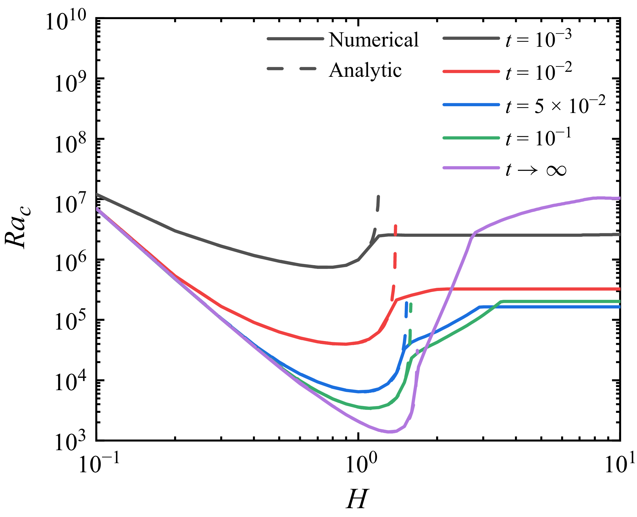
The eigenproblem (3.8) can also be solved numerically using the Chebyshev collocation spectral method (Zhou & Li Reference Zhou and Li2017; Zhou, Sun & Li Reference Zhou, Sun and Li2022; Shankar & Shivakumara Reference Shankar and Shivakumara2023). Grid-independent results are attained with 50 nodes for most configurations. As shown in figure 2, the numerical and analytical solutions of (3.8) are in excellent agreement until
 $H$
exceeds a critical value. This discrepancy arises because the minimum positive eigenvalue of (3.8) does not occur in the limit
 $k^2 \rightarrow 0$
. In such cases, the asymptotic expansion (3.10) is no longer applicable. The observed inconsistency can be attributed to the localisation of the instability at large
 $H$
, where the stable interlayer, rather than the top and bottom boundaries, acts as the effective boundaries for the unstable layers (Farrow & Patterson Reference Farrow and Patterson1993). Consequently, the characteristic vertical scale of the instability is effectively reduced – a behaviour that is corroborated by the local
 $\textit{Ra}$
model presented in § 3.2.
According to figure 2,
 $\textit{Ra}_c$
exhibits a non-monotonic dependence on
 $H$
, first decreasing and then increasing. For small
 $H$
,
 $\textit{Ra}_c$
decreases monotonically with time, asymptotically approaching a minimum value as
 $t \rightarrow \infty$
. For large
 $H$
, it first decreases to a minimum before increasing. Thus, we define the upper and lower bounds of
 $\textit{Ra}_c$
as
 \begin{equation} \left \{ \begin{array}{ll}\!\! \textit{Ra}_{c,u}(H,\phi ) = \textit{Ra}_c(H,\phi , t \rightarrow \infty ), \\[3pt] \!\!\textit{Ra}_{c,l}(H,\phi ) = \min \limits _{t}\left \{\textit{Ra}_c(H,\phi , t)\right \}\!. \end{array} \right . \end{equation}
Comparison of the numerical and analytic solutions of eigenproblem (3.8) for
 $\phi =0.1$
.

Three distinct stability regimes are identified based on the applied
 $\textit{Ra}$
. The flow remains unconditionally stable for
 $\textit{Ra} \lt \textit{Ra}_{c,l}$
and permanently unstable for
 $\textit{Ra} \gt \textit{Ra}_{c,u}$
. In the intermediate range
 $\textit{Ra}_{c,l} \leq \textit{Ra} \leq \textit{Ra}_{c,u}$
, the system exhibits transient instability: it becomes unstable once the time-dependent critical value
 $\textit{Ra}_c(t)$
decreases below the applied
 $\textit{Ra}$
and restabilises when
 $\textit{Ra}_c(t)$
increases above it. A detailed analysis of these regimes is provided in § 4.2.
It should be emphasised that the obtained
 $\textit{Ra}_{c,l}$
is the theoretical minimum for the onset of any instability. In practice, however, the threshold for manifest convection generally exceeds this theoretical value. To illustrate this distinction, let
 $\textit{Ra}_{c,l} = \textit{Ra}_c(t_1)$
. Although an applied
 $\textit{Ra} \gt \textit{Ra}_c(t_1)$
triggers linear instability at
 $t = t_1$
, a finite time is required for perturbations to amplify into manifest convection. Consequently, if manifest convection has not been observed by a later time
 $t_2 \gt t_1$
under
 $\textit{Ra} = \textit{Ra}_c(t_2)$
, the flow will remain stable thereafter. This behaviour stems from the monotonic increase of
 $\textit{Ra}_c(t)$
for
 $t \gt t_1$
, which prevents the applied
 $\textit{Ra}$
from re-entering the unstable regime.
3.1.2. Amplification theory
The linear stability equations (3.6) admit solutions in the form of a Fourier cosine series (Foster Reference Foster1965):
 \begin{equation} \hat {T}(z,t) = \sum _{m=1}^{N}A_m(t) \cos \left (\frac {2m\pi }{H}z\right )\!, \end{equation}
a representation that also describes the initial perturbations and inherently satisfies the temperature boundary conditions (3.7).
Numerical solutions are obtained using the Chebyshev collocation spectral method with a first-order implicit time discretisation. The evolution of perturbations is quantified by the amplification factor
 $E_T(t)$
, defined as the normalised
 $L_2$
energy norm of the temperature perturbation:
 \begin{equation} E_T(t) = \left [ \frac {\int _{-H}^{0}\hat {T}^2 (z,t) \mathrm{d}z}{\int _{-H}^{0}\hat {T}^2 (z,0) \mathrm{d}z} \right ]^{\tfrac {1}{2}}\!. \end{equation}
A comparison of the initial perturbation profiles is presented in figure 3. The ‘single mode’ perturbation initialises one Fourier coefficient to unity while setting all others to zero, whereas the ‘white noise’ perturbation initialises all coefficients to unity. Results from both approaches are found to be broadly consistent. Therefore, for simplicity, only the ‘single mode’ initialisation is employed in the subsequent analysis.
Growth of instabilities under various initial conditions for
 $k = 1$
,
 $\textit{Ra} = 10^9$
,
 $\textit{Pr} = 7$
,
 $H = 2$
and
 $\phi = 0.2$
. The initial perturbations are characterised by the Fourier mode
 $m$
and the series truncation level
 $N$
.

Theoretically, the upper critical Rayleigh number
 $\textit{Ra}_{c,u}$
can be determined by the marginal stability condition
 $\partial _t E_T(t \to \infty ) = 0$
. However, in practice,
 $E_T(t)$
may decay to levels comparable to numerical noise and subsequently exhibit unphysical growth or oscillations. To mitigate such spurious behaviour, we adopt a more robust criterion
 $E_T(t \to \infty ){}= 1$
. Analogously, the lower bound
 $\textit{Ra}_{c,l}$
is identified as
 $\textit{Ra}$
for which
 $E_T(t) = 1$
is first satisfied at some finite time
 $t\gt 0$
. Accordingly,
 $\textit{Ra}_c$
is defined as
 \begin{equation} \textit{Ra}_c \left (H, \phi , t \right )=\underset {\substack {k,m \\E_T(t)=1}}{\min } \left \{\textit{Ra} \big (k^2, H, \phi , t \big ) \right \}\!, \end{equation}
and is computed numerically via the bisection method.
For given
 $\textit{Ra}$
,
 $\phi$
and
 $H$
, the critical time
 $t_c$
for flow onset is defined as the shortest time
 $t$
at which the amplification factor
 $E_T(t)$
first reaches a threshold of 1000, minimised over all wavenumbers
 $k$
and mode indices
 $m$
. This leads to the minimisation problem:
 \begin{equation} t_c=\underset {\substack {k, m}}{\min } \left \{t \mid E_T(t)=1000 \right \}\!, \end{equation}
which we solve using the particle swarm optimisation (PSO) algorithm (Kennedy & Eberhart Reference Kennedy and Eberhart1995). The choice of threshold,
 $E_T(t) = 1000$
, follows Kaviany (Reference Kaviany1984). In practice, the computed
 $t_c$
depends only weakly on the specific threshold value, due to the high growth rate of the underlying instability (Jaupart & Parsons Reference Jaupart and Parsons1985).
3.2. Local Ra model
Although radiation-induced convection differs fundamentally from the classical Rayleigh–Bénard configuration, the two systems can exhibit similar linear instability characteristics. To quantify this similarity, we introduce a Rayleigh number based on the temperature difference across the layer:
 \begin{equation} \textit{Ra}_T = \frac {\beta g \Delta T^* H^{*3}}{\nu a}, \end{equation}
which, in dimensionless form, becomes
 \begin{equation} \textit{Ra}_T = \textit{Ra} \Delta T H^3. \end{equation}
Here,
 $\Delta T^*$
and
 $\Delta T$
denote the dimensional and dimensionless temperature differences between the top and bottom boundaries, respectively.
By combining (3.1), (3.12) and (3.21), and applying a Taylor expansion for the limiting case
 $H \ll 1$
,
 $t \to \infty$
, we obtain the asymptotic expressions:
 \begin{equation} \textit{Ra}_c = \frac {576}{(0.8+\phi )H^4} \end{equation}
and
 \begin{equation} \textit{Ra}_{\textit{Tc}} = \frac {288(1+\phi )}{0.8+\phi }. \end{equation}
Equation (3.23) provides two asymptotic bounds, 288 and 360, which agree with the results reported by Goluskin (Reference Goluskin2015) for analogous configurations. Specifically, in the framework of Goluskin (Reference Goluskin2015):
-
(i) a rigid fixed-heat-flux top and a free-slip diabatic bottom yield a
 $\textit{Ra}_{\textit{Tc}}$
of 720;
-
(ii) a free-slip fixed-heat-flux top and a rigid diabatic bottom give 576;
-
(iii) a free-slip fixed-heat-flux top and a free-slip diabatic bottom lead to 240.

Note that the characteristic temperature scale used by Goluskin (Reference Goluskin2015) is twice the actual temperature difference between the top and bottom boundaries. Therefore, when recast in terms of the
 $\textit{Ra}_T$
defined in (3.20), these three configurations correspond to
 $\textit{Ra}_{\textit{Tc}} = 360$
, 288 and 120, respectively. The first two values represent the limiting regimes of the present convection system: the case of pure surface cooling (
 $\phi \gg 1$
) and the case dominated by bottom heating (
 $\phi \to 0$
,
 $H \ll 1$
).
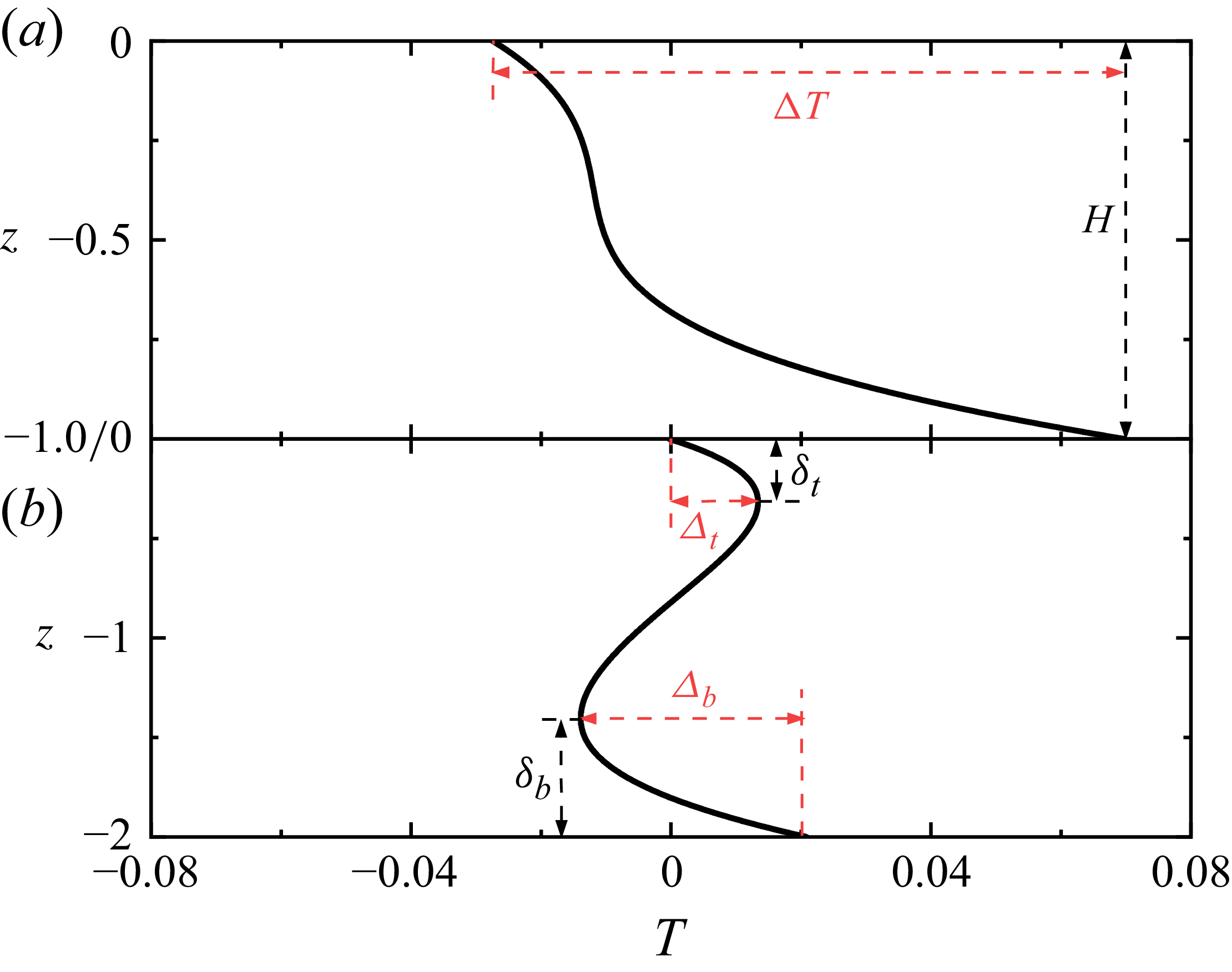
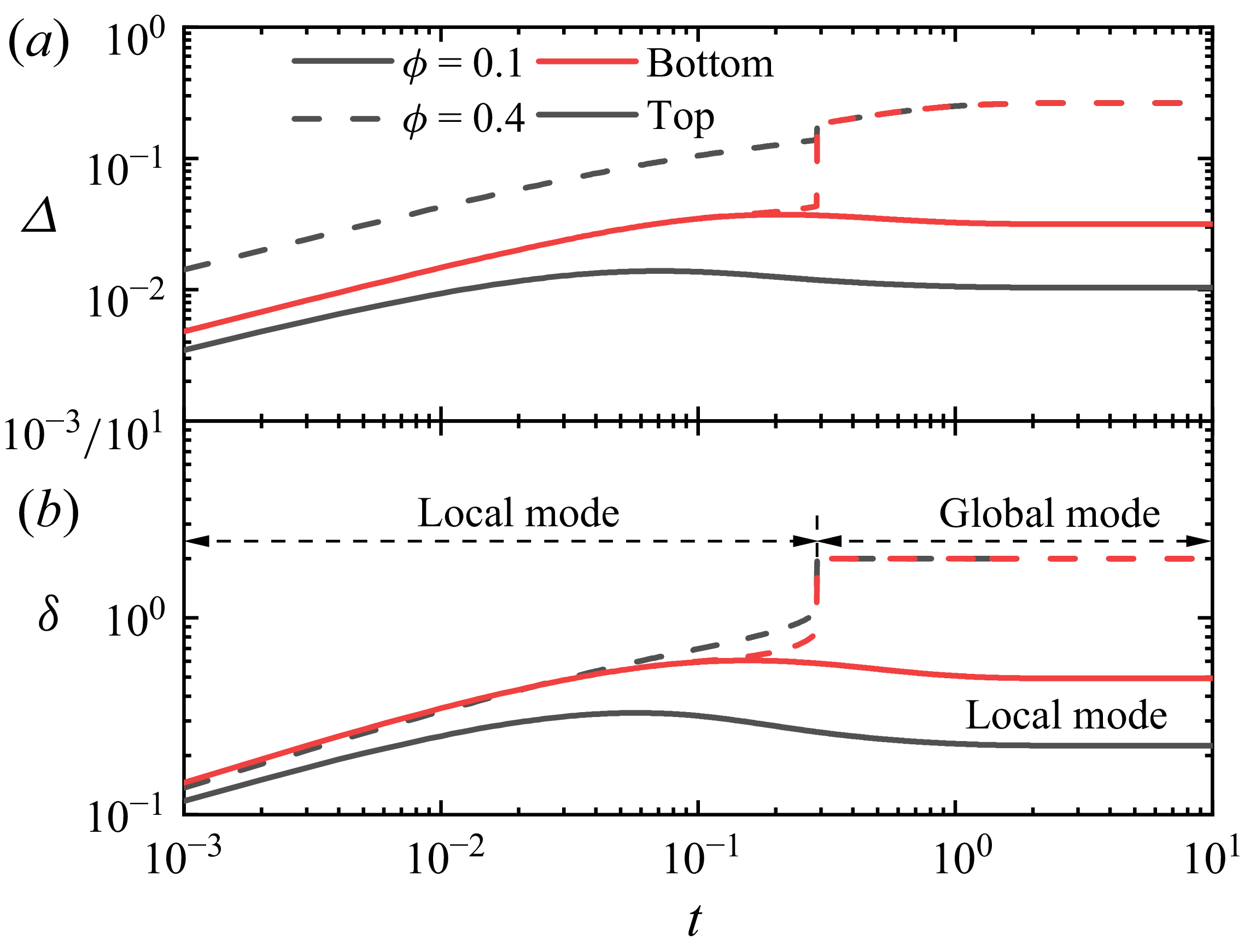
The static temperature profile (3.1) supports two distinct instability modes, shown schematically in figure 4: the global mode and the local mode. In the global mode, the temperature decreases monotonically with height and the instability scale is the full fluid depth
 $H$
. Instability occurs when the applied
 $\textit{Ra}$
exceeds
 $\textit{Ra}_c$
, with
 $\textit{Ra}_c$
given explicitly by (3.12). In contrast, local instability develops within the TBLs bounded by the physical boundaries and the local temperature extrema, separated by a stable interlayer with a positive vertical temperature gradient. The instability in this case is controlled by the TBL thickness
 $\delta$
and the onset criterion is expressed in terms of the local Rayleigh number:
 \begin{equation} \textit{Ra}_{\textit{TL}} = \textit{Ra} \varDelta \delta ^3 \geqslant \textit{Ra}_{\textit{Tc}}, \end{equation}
where
 $\varDelta$
is the temperature difference across the TBL. The stable interlayer acts as an effective free-slip adiabatic boundary for each TBL, yielding critical local Rayleigh numbers of
 $\textit{Ra}_{\textit{Tc}} = 120$
for the top TBL and
 $\textit{Ra}_{\textit{Tc}} = 360$
for the bottom TBL.
Temperature distributions for: (a) global instability mode where
 $H=1$
,
 $\phi =0.1$
and
 $t=0.05$
; (b) local instability mode where
 $H=2$
,
 $\phi =0.1$
and
 $t=0.1$
.

The thickness and temperature difference of each TBL can be directly obtained from the conductive temperature profile in (3.1). Together with the instability mode identified from the TBL thickness (see figure 5),
 $\textit{Ra}_c$
can be evaluated:
 \begin{align} \textit{Ra}_c =\left \{ \begin{array}{ll}\!\! \frac {48H}{A+B}, \quad \delta = H, \\[7pt] \!\! \min \left \{\frac {120}{\varDelta _t \delta _t^3},\frac {360}{\varDelta _b \delta _b^3} \right \}\!, \quad \delta \neq H, \end{array} \right . \end{align}
where subscripts
 $(\boldsymbol{\cdot })_t$
and
 $(\boldsymbol{\cdot })_b$
denote the top and bottom TBLs, respectively.
(a) Temperature differences, and (b) thicknesses of the top and bottom TBLs, along with the identified instability modes, as derived from the conductive temperature profile.

3.3. Scaling analysis
At the initial stage (
 $t \to 0$
), the fluid is motionless. In the vicinity of the top boundary, the volumetric heat source is approximately constant. Consequently, the energy equation (2.13) reduces to a balance between thermal inertia and conduction:
 \begin{equation} \frac {\varDelta _t}{t} \sim \frac {\varDelta _t}{\delta _t^2}, \end{equation}
where the contribution of the heat source vanishes because, to leading order, it heats the fluid within the boundary layer uniformly and thus does not contribute to the local temperature difference. That is, the top TBL grows diffusively as
 \begin{equation} \delta _t \sim \sqrt {t}. \end{equation}
This growth continues until the onset of convective motion, at which point both
 $\delta _t$
and
 $\varDelta _t$
attain their maximum values and
 $\partial _t \varDelta _t = 0$
. The energy balance in (2.13) then simplifies to
 \begin{equation} w_t\frac {\varDelta _t}{\delta _t} \sim \frac {\varDelta _t}{\delta _t^2}. \end{equation}
The thermal boundary condition (2.15) yields
 \begin{equation} \frac {\varDelta _t}{\delta _t} \sim \phi . \end{equation}
The momentum equation (2.12) reflects a balance among inertia, viscous friction and buoyancy:
 \begin{equation} \frac {w_t}{t}+\frac {w_t^2}{\delta _t} \sim -\textit{Pr}\frac {w_t}{\delta _t^2} + \textit{RaPr} \varDelta _t. \end{equation}
Combining (3.27)–(3.30) leads to the scaling for the critical time for flow onset at the top boundary:
 \begin{equation} t_{c,t} \sim \left (\frac {\textit{RaPr}\phi }{2+\textit{Pr}}\right )^{-1/2}. \end{equation}
A similar procedure yields the scaling for the bottom boundary:
 \begin{equation} t_{c,b} \sim \left [\frac {\textit{RaPr}\exp (-H)}{2+\textit{Pr}}\right ]^{-1/2}. \end{equation}
The overall critical time
 $t_c$
is then given by the minimum of the two:
 \begin{equation} t_c = \min \left \{ t_{c,t},\ t_{c,b} \right \}. \end{equation}
From (3.31) and (3.32), the dependence of
 $t_c$
on
 $\textit{Pr}$
follows the scaling
 \begin{equation} t_c \sim \left \{ \begin{array}{ll}\!\! \textit{Pr}^{-1/2}, \quad \textit{Pr} \ll 1, \\[3pt] \!\! \textit{Pr}^0, \quad \textit{Pr} \gg 1. \end{array} \right . \end{equation}
An alternative estimate can be obtained from the local
 $\textit{Ra}$
criterion. Substituting the TBL scaling from (3.27) and the temperature scaling from (3.29) into the local criterion (3.24) yields
 \begin{equation} t_{c,t} \sim \sqrt {\frac {120}{\textit{Ra} \phi } }, \end{equation}
and similarly for the bottom boundary,
 \begin{equation} t_{c,b} \sim \sqrt {\frac {360}{\textit{Ra} \exp \left (-H \right )} }. \end{equation}
These expressions are structurally similar to (3.31) and (3.32), differing primarily in their dependence on
 $\textit{Pr}$
. This distinction reflects a key physical difference: (3.31) and (3.32) characterise the onset time for manifest convection, whereas (3.35) and (3.36) correspond to the onset of flow instability.
4. Validation by direct numerical simulations
The theoretical predictions presented earlier are validated against two-dimensional DNS of flow in a horizontal fluid layer. The computational domain has a fixed horizontal length of
 $L = 4$
, while the depth
 $H$
varies over the range
 $0.5 \leqslant H \leqslant 3$
.
4.1. Numerical method and codes validation
The DNSs are performed using the open-source framework Dedalus (Burns et al. Reference Burns, Vasil, Oishi, Lecoanet and Brown2020). The governing equations (2.10)–(2.13), and boundary conditions (2.14) and (2.15) are discretised spectrally using the tau method, with Fourier series in the horizontal direction and Chebyshev polynomials in the vertical direction. A
 $3/2$
dealiasing rule is applied in both directions. Time discretisation is carried out via a Crank–Nicolson/Adams–Bashforth scheme with an adaptive time step, constrained by a CFL condition with a maximum value of 0.2. To ensure accurate determination of
 $t_c$
, the time step is further restricted to values below
 $10^{-6}$
. A random noise perturbation of amplitude
 $10^{-5}$
is superimposed on the initial temperature field.
In the DNS,
 $\textit{Ra}_c$
is determined by monitoring the temporal evolution of the maximum velocity in the domain. A sustained growth in the velocity signals the onset of instability and
 $\textit{Ra}_c$
is located using a bisection method with a relative precision of
 $1\,\%$
. For a given set of parameters,
 $t_c$
is extracted by tracking the evolution of the temperature difference between the top and bottom boundaries. Specifically,
 $t_c$
is defined as the bifurcation point at which the DNS results depart from the pure conductive solution and this point is identified using the tangent method. The use of separate criteria for
 $\textit{Ra}_c$
and
 $t_c$
is motivated by their distinct underlying physics. Velocity is employed to determine
 $\textit{Ra}_c$
because the incipient flow near the critical threshold is too weak to perturb the conductive temperature profile appreciably, rendering velocity a more sensitive and reliable indicator of instability. In contrast, the tangent method applied to velocity is unsuitable for detecting
 $t_c$
, as the velocity magnitude spans a large dynamic range with
 $\textit{Ra}$
. The temperature difference, by contrast, exhibits smaller variation and admits a theoretical prediction (Zhou et al. Reference Zhou, Yang, You, Liu, Sun and Li2025), offering a more accurate and consistent measure for determining
 $t_c$
.
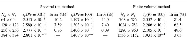
A systematic grid-independence test is conducted to verify the adequacy of the numerical resolution. Four grid resolutions (
 $N_x \times N_z$
) are evaluated for the most computationally demanding parameter combination (
 $\textit{Ra} = 10^{10}$
,
 $\phi = 0.7$
,
 $H = 3$
), covering two extreme Prandtl numbers (
 $\textit{Pr} = 0.01$
and
 $100$
) that exhibit the highest sensitivity to grid resolution. As summarised in table 1, the critical time
 $t_c$
converges monotonically with grid refinement. Relative to the benchmark set by the finest grid (
 $384 \times 384$
), the relative error for the
 $256 \times 256$
grid is within
 $1\,\%$
. Consequently, this resolution is adopted for all subsequent DNS runs, ensuring grid-independent results across the entire parameter space investigated in the present study. Furthermore, the performance of the spectral tau method is compared against a second-order finite volume method (FVM) at
 $\textit{Pr} = 100$
. When the
 $384 \times 384$
spectral tau solution is used as the reference, the FVM results exhibit significantly larger deviations even at substantially higher resolutions. This stark contrast highlights the superior accuracy and efficiency of the spectral tau method, thereby justifying its adoption in the present study.
Grid-independence test and method comparison for the critical time
 $t_c$
at
 $\textit{Ra} = 10^{10}$
,
 $\phi = 0.7$
and
 $H = 3$
. The reference solution used to compute the relative errors entails the spectral tau method evaluated on a
 $384 \times 384$
grid.

To validate the DNS methodology, we simulate the classical Rayleigh–Bénard convection system heated from below with a constant heat flux, a configuration that has been extensively studied both experimentally and theoretically (Nielsen & Sabersky Reference Nielsen and Sabersky1973; Chu Reference Chu1990; Choi et al. Reference Choi, Park, Kim, Lee, Kim and Davis2004). The working fluids considered in those experiments include silicone oils (
 $\textit{Pr} = 45$
, 896, 4700) and syrup (
 $\textit{Pr} = 4.5 \times 10^5$
) (Nielsen & Sabersky Reference Nielsen and Sabersky1973; Chu Reference Chu1990). Choi et al. (Reference Choi, Park, Kim, Lee, Kim and Davis2004) employed propagation theory in the infinite-Prandtl-number limit to predict
 $t_c$
, reporting results that agree with experimental data to within a factor of 3.2. As shown in figure 6, our DNS results, together with predictions from amplification theory, are in excellent agreement with the published data. Furthermore, consistent with the scaling relation (3.34) derived for the present system,
 $t_c$
in the Rayleigh–Bénard configuration is found to be essentially independent of
 $\textit{Pr}$
for
 $\textit{Pr} \gg 1$
. The dimensionality of the simulation (two-dimensional (2-D) versus three-dimensional (3-D)) is also verified to have a negligible influence on the predicted onset time.
Validation of
 $t_c$
from DNS and amplification theory against literature data.

4.2. Critical Rayleigh number
Figure 7 presents the critical Rayleigh number
 $\textit{Ra}_c$
obtained from the marginal stability assumption as a function of
 $H$
for various cooling parameters
 $\phi$
. A monotonic decrease in
 $\textit{Ra}_c$
is observed with increasing
 $\phi$
. For
 $H \lt 1$
,
 $\textit{Ra}_c$
can be accurately predicted by (3.22). The bifurcation into the upper bound
 $\textit{Ra}_{c,u}$
and the lower bound
 $\textit{Ra}_{c,l}$
occurs for
 $H \gt 1$
. As
 $H$
increases,
 $\textit{Ra}_{c,l}$
forms a plateau, while the dependence of
 $\textit{Ra}_{c,u}$
on
 $H$
gradually weakens. This behaviour can be explained by the mechanism of local instability. For both
 $\phi = 0$
and
 $\phi = 0.1$
, the lower bounds
 $\textit{Ra}_{c,l}$
coincide over a range of
 $H$
, indicating that instability in this regime is governed primarily by bottom heating. As
 $H$
increases, the heat flux reaching the bottom wall diminishes. For non-adiabatic surfaces (
 $\phi \gt 0$
), instability eventually becomes dominated by surface cooling, leading to an
 $\textit{Ra}_{c,l}$
that is independent of
 $H$
. In contrast, the dependence of
 $\textit{Ra}_{c,u}$
on
 $H$
stems from the long-term influence of bottom heating on the temperature distribution near the top boundary – an effect that weakens as
 $H$
increases.
(a) Bounds of
 $\textit{Ra}_c$
and (b) the corresponding values compensated by the factor
 $576/(0.8+\phi )$
, plotted as functions of
 $H$
for various
 $\phi$
, obtained from the marginal stability assumption.

Figure 8 compares the bounds
 $\textit{Ra}_{c,l}$
and
 $\textit{Ra}_{c,u}$
obtained by different methods. Note that the results from the marginal stability assumption and local
 $\textit{Ra}$
model are
 $\textit{Pr}$
-independent, whereas those from the amplification theory and DNS are obtained at
 $\textit{Pr}=7$
. Overall, good agreement is observed across all methods, with the exception of the DNS results at large
 $H$
. The comparison further shows that
 $\textit{Ra}_{c,l}$
predicted by the marginal stability assumption is slightly lower than the values obtained from transient approaches, whereas excellent agreement is found for
 $\textit{Ra}_{c,u}$
. This discrepancy arises because the transient determination of
 $\textit{Ra}_{c,l}$
requires perturbations to amplify to a detectable level within a finite time, whereas
 $\textit{Ra}_{c,u}$
corresponds to a fully developed instability approached asymptotically at long times. Notably, the local
 $\textit{Ra}$
model exhibits good accuracy, offering a simple yet effective tool for predicting
 $\textit{Ra}_c$
for the onset of flow in penetrative convection.
Comparison of
 $\textit{Ra}_c$
obtained using different methods: (a) upper bound
 $\textit{Ra}_{c,u}$
; (b) lower bound
 $\textit{Ra}_{c,l}$
.

Typical flow regimes under different
 $\textit{Ra}$
, where
 $\textit{Pr} = 7$
,
 $H = 3$
and
 $\phi = 0.1$
: (a) discrepancy between the DNS and conductive solutions in the temperature difference across the boundaries; (b) temporal evolution of the maximum velocity magnitude.

For
 $H=3$
and
 $\phi =0.1$
, the marginal stability analysis yields the lower and upper critical bounds as
 $\textit{Ra}_{c,l}=120\,256$
and
 $\textit{Ra}_{c,u}=3\,269\,349$
, respectively. To illustrate the distinct flow regimes delineated by these bounds, we perform DNS and examine the evolution of both the top-bottom temperature difference and the maximum velocity magnitude at three representative Rayleigh numbers:
 $10^5$
,
 $10^6$
and
 $5 \times 10^6$
. Figure 9 illustrates the resulting flow regimes in the convection system driven by radiation absorption and surface cooling. At
 $\textit{Ra} = 10^5$
, which lies below
 $\textit{Ra}_{c,l}$
, the system remains stable and the temperature difference closely matches the conductive profile. For
 $\textit{Ra}$
above
 $\textit{Ra}_{c,l}$
, the DNS temperature difference initially agrees well with the conductive solution. As heating continues, however, flow instability develops, leading to a growing departure from the conductive solution. At
 $\textit{Ra} = 10^6$
, the temperature difference deviation rises rapidly from zero to a maximum, then decreases sharply and eventually returns to nearly zero. Correspondingly, the maximum velocity rises from zero to a peak before decaying back to zero. This behaviour reflects a transient growth of instability, where the flow temporarily departs from the conductive state but is eventually suppressed – confirming that this
 $\textit{Ra}$
exceeds the lower bound but remains below the upper bound. In contrast, at
 $\textit{Ra} = 5 \times 10^6$
, both the temperature difference deviation and the maximum velocity converge to non-zero steady values, indicating sustained, albeit relatively weak, convection. This confirms that the applied
 $\textit{Ra}$
exceeds the upper critical bound. Additionally, the supplementary material provide visualisations of this transient behaviour at
 $\textit{Ra} = 10^6$
, showing the transient onset and subsequent suppression of convection (see supplementary movies 1–3 available at https://doi.org/10.1017/jfm.2026.11498, which display the evolving temperature contours for the 2-D configuration, the 3-D configuration and a 2-D cross-section taken from the 3-D domain, respectively).
4.3. Critical time for flow onset
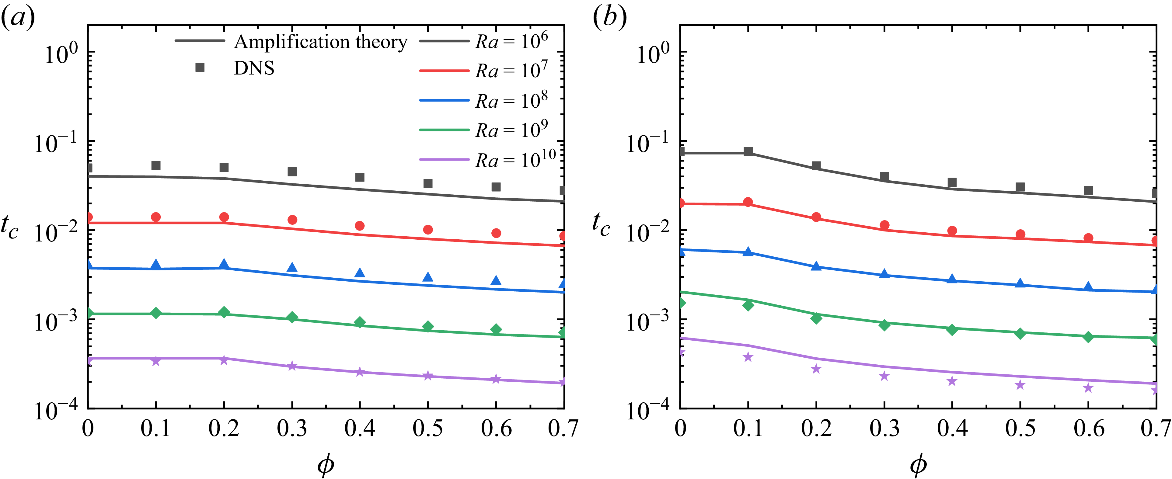
Figure 10 compares the critical time
 $t_c$
for flow onset predicted by amplification theory and DNS at two fluid depths: (a)
 $H = 1$
and (b)
 $H = 2$
. The two approaches demonstrate excellent agreement, both in the absolute values and in the functional dependence on the parameters. As expected,
 $t_c$
decreases with increasing
 $\textit{Ra}$
. The dominant triggering mechanism transitions from bottom-heating control at low
 $\phi$
, where
 $t_c$
is largely independent of
 $\phi$
, to surface-cooling control at higher
 $\phi$
, which systematically reduces
 $t_c$
. This regime transition occurs near
 $\phi = 0.2$
for
 $H = 1$
and near
 $\phi = 0.1$
for
 $H = 2$
. To clearly distinguish between the two triggering mechanisms in subsequent analyses, we adopt
 $H = 2$
with
 $\phi \geqslant 0.1$
to represent surface-cooling-driven onset and
 $\phi = 0$
for bottom-heating-driven onset.
Critical time
 $t_c$
for flow onset as a function of
 $\phi$
and
 $\textit{Ra}$
for
 $\textit{Pr} = 7$
: (a)
 $H = 1$
; (b)
 $H = 2$
.

To isolate the surface-cooling- and bottom-heating-driven regimes, we adopt distinct parameter sets and examine the collapse of the critical time data. Figure 11 plots
 $t_c$
against the rescaled surface cooling flux
 $\textit{Ra} \textit{Pr} \phi / (2+\textit{Pr} )$
and bottom heating flux
 $\textit{Ra} \textit{Pr} \exp (-H ) / (2+\textit{Pr} )$
, spanning the ranges
 $10^6\leqslant \textit{Ra} \leqslant 10^{10}$
,
 $0.07\leqslant \textit{Pr} \leqslant 70$
,
 $0\leqslant \phi \leqslant 0.7$
and
 $0.5\leqslant H \leqslant 3$
. Under this rescaling, all data points collapse onto a master curve exhibiting a scaling law with slope
 $-1/2$
, thereby confirming the theoretical relations (3.31) and (3.32). Enforcing a slope of
 $-1/2$
, a least-squares fit yields
 \begin{equation} \left \{ \begin{array}{ll} \!\! t_{c,t}=15.30\times \left (\frac {\textit{RaPr}\phi }{2+\textit{Pr}}\right )^{-1/2}, \\[9pt] \!\! t_{c,b}=19.20\times \left [\frac {\textit{RaPr}\exp (-H)}{2+\textit{Pr}}\right ]^{-1/2}. \end{array} \right . \end{equation}
Scaling law for
 $t_c$
: (a) surface-cooling-driven onset (
 $H = 2$
); (b) bottom-heating-driven onset (
 $\phi = 0$
).

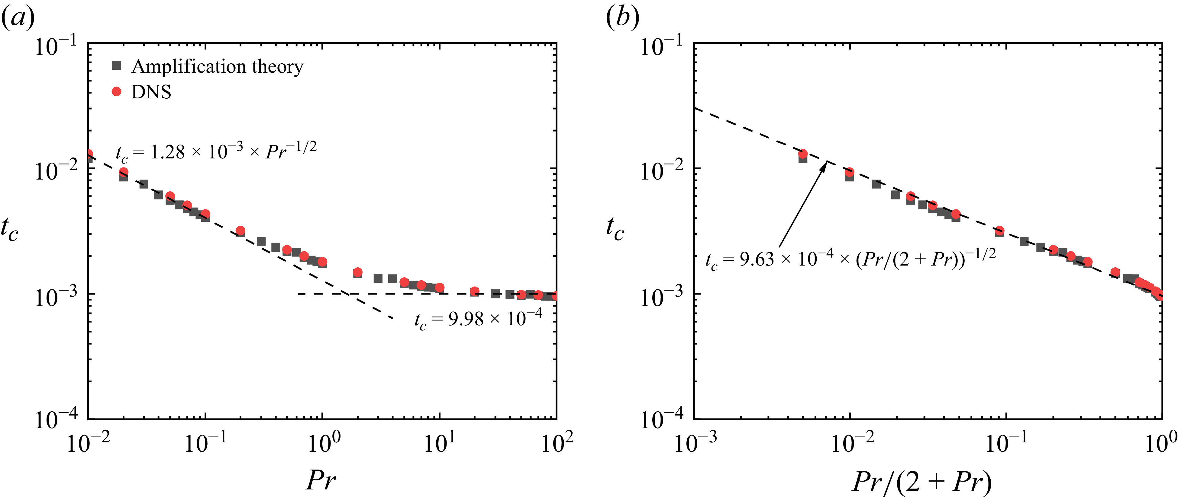
To further examine the
 $\textit{Pr}$
-scaling relation (3.34), figure 12 presents results over a wider span of
 $\textit{Pr}$
, under fixed conditions
 $\textit{Ra} = 10^9$
,
 $H=1$
and
 $\phi =0$
. Figure 12(a) shows the variation of
 $t_c$
with
 $\textit{Pr}$
: for low
 $\textit{Pr}$
, the scaling approaches
 $t_c \sim \textit{Pr}^{-1/2}$
, while for high
 $\textit{Pr}$
, it asymptotes to
 $t_c \sim \textit{Pr}^{0}$
. A unified scaling is proposed using the group
 $\textit{Pr}/(2+\textit{Pr})$
, as shown in figure 12(b). In this representation,
 $t_c$
scales with
 $\textit{Pr}/(2+\textit{Pr})$
and exhibits an exponent close to
 $-1/2$
.
Validation of the scaling relationship between
 $t_c$
and
 $\textit{Pr}$
, where
 $\textit{Ra} = 10^9$
,
 $\phi = 0$
and
 $H = 1$
: (a) scaling relationship between
 $t_c$
and
 $\textit{Pr}$
; (b) scaling relationship between
 $t_c$
and
 $\textit{Pr}/(2+\textit{Pr})$
.

5. Conclusions
This study investigates the transient stability of natural convection driven by coupled radiation absorption and surface cooling. We address two fundamental questions: the determination of the critical Rayleigh number
 $\textit{Ra}_c$
for convection onset from a static state and the quantification of the corresponding critical time
 $t_c$
for flow onset required for flow development beyond this threshold.
For
 $\textit{Ra}_c$
, we employ two LSA frameworks: a quasi-steady approach based on the marginal stability assumption applied to the instantaneous static state and a transient growth approach using amplification theory with the criterion
 $E_T \geqslant 1$
for instability onset. The analysis reveals a remarkable flow suppression phenomenon in deep fluid layers, leading to the identification of dual critical thresholds: an upper bound,
 $\textit{Ra}_{c,u}$
, above which convective flow sustains indefinitely, and a lower bound,
 $\textit{Ra}_{c,l}$
, at which flow onset occurs at a finite time. To predict these thresholds efficiently, a local
 $\textit{Ra}$
model is developed. Relying solely on the conductive temperature profile, this model directly bridges the stability criteria of our system with those of the classical Rayleigh–Bénard problems. It demonstrates excellent predictive capability and shows immediate potential for extension to other penetrative convection systems with similar suppression mechanisms. All theoretical predictions for
 $\textit{Ra}_c$
have been conclusively validated against DNS.
For
 $t_c$
, the validity of the adopted amplification criterion has been rigorously established, identifying
 $t_c$
as the time when the amplification factor reaches
 $E_T \geqslant 1000$
. This threshold effectively represents the transition from infinitesimal instability to manifest convection, accounting for the finite time required for perturbations
 $E_T$
to amplify from
 $E_T=1$
to
 $E_T=1000$
. The predictions of amplification theory are in excellent agreement with our DNS. Furthermore, through systematic scaling analysis, we have established explicit scaling laws connecting
 $t_c$
with key governing parameters, providing a comprehensive predictive framework for convective initiation across a wide range of physical conditions.
The physical configuration considered here, with its coupled radiation absorption and surface cooling, represents a fundamental paradigm for numerous natural and engineering systems, including atmospheric and oceanic circulation, solar ponds, and direct absorption solar collectors. While the present study focuses on an idealised case with fixed heating and cooling conditions, future work could incorporate more realistic factors such as diurnal solar radiation cycles (Chang & Scotti Reference Chang and Scotti2023), Taylor–Proudman effect (Leng et al. Reference Leng, Krasnov, Li and Zhong2021) and spectrally selective absorption (Du & He Reference Du and He2024).
Supplementary movies
Supplementary movies are available at https://doi.org/10.1017/jfm.2026.11498.
Funding
This work was supported by the National Natural Science Foundation of China (Nos. 52206103, 52306069, and 52476156) and the Shanghai Sailing Program (No. 21YF1430400).
Declaration of interests
The authors declare no conflict of interest.
Data availability statement
Data available on request from the corresponding author.
Declaration of AI assistance
The authors acknowledge the use of DeepSeek, an AI language model developed by DeepSeek Company, solely for the purpose of improving language fluency, clarity and academic style during the writing process. This tool was used for linguistic refinement and did not contribute to the generation of scientific ideas, data analysis or theoretical interpretations. The authors are solely responsible for the research content, findings and conclusions presented in this work.