





1. Introduction
We report the results of an experimental investigation into the slow motion of large rigid spheres through a highly deformable soft solid. The soft material comprises a highly concentrated collection of fully hydrated hydrogels immersed in water. The particle concentration is such that the swollen particles form a dense packing in the form of an interconnected network of highly elastic, porous material with no detectable connected regions of water in the interior or at the surface of the sample. The water maintains the hydrogels at an equilibrium swelling condition; hence, attractive forces between fully swollen hydrogel spheres are minimal: the chemical potential difference (Yoon et al. Reference Yoon, Cai, Suo and Hayward2010) between neighbouring, fully swollen particles, which may induce a negative solvent pressure, is assumed to be small. The material response of such packings is known to comprise both fluid-like rate dependence and solid-like elasto-plastic resistance. Hence, an embedded intruder that moves through the material will experience a drag force as a result of elasto-plastic deformation. Moreover, the material is compressed and expands smoothly as the intruder passes through the packing. Applications of such materials are wide ranging and can be found in soft robotics and soil sciences; see, for example, Tabuteau et al. (Reference Tabuteau, Sikorski and de Bruyn2007b ).
In the laboratory, submersed hydrogel particle packings are contained within well-defined boundaries. The two-phase material comprises water and hydrogel spheres. Each component responds differently to end boundaries: specifically, no-slip applies to the water along rigid walls but the particles slip with respect to any surface. In the sample creation process, the dry particles are added to water and they swell and settle into a submersed bed. We have shown that the particle packing boundary has a significant effect on the mechanical properties of the medium. Specifically, an external pressure exerted on the particle boundary exponentially affects the drag forces of an intruder moving through the sample (Dijksman & Mullin Reference Dijksman and Mullin2022, Reference Dijksman and Mullin2024b ). Here we now show that the presence of a free surface has a dramatic effect on the drag force. While a rigid end imposed on the boundary orthogonal to the imposed stress induces a time dependence in the speed of an intruder driven at constant stress, a free boundary condition allows an intruder under constant stress to attain a constant ‘terminal’ velocity. As previously reported by Pal & Kudrolli (Reference Pal and Kudrolli2021), the flow field around a moving intruder inside a hydrogel packing is highly localised at the sides of the moving intruder. However, here we find that the deformation field in front of the intruder affects the end boundary shape significantly when it is free.
Intruders moving under constant stress conditions have been used in the past to provide insights into the flow behaviour of non-Newtonian fluids, such as viscoelastic materials (Cho et al. Reference Cho, Hartnett and Lee1983; Tabuteau et al. Reference Tabuteau, Coussot and de Bruyn2007a
; Sgreva et al. Reference Sgreva, Davaille, Kumagai and Kurita2020). For example, in a study of a shear thinning fluid it is found that the distance the sphere travels is
 $\propto t^{1/2}$
(McKinley Reference McKinley2002). An explanation for this nonlinear behaviour is provided by Beris et al. (Reference Beris, Tsamopoulos, Armstrong and Brown1985) who postulate that a build up of stagnant fluid around the sphere will lead to an increase in its effective size over time and, hence, the drag force increases accordingly. In shear thickening fluids, a similar coupling has been observed between the effective size of the intruder and the viscous response of the material surrounding it for the nonlinear slowdown of an intruder (Brassard et al. Reference Brassard, Causley, Krizou, Dijksman and Clark2021), which may lead to oscillatory velocity fluctuations (von Kann et al. Reference von Kann, Snoeijer and van der Meer2013). These examples highlight that, for non-Newtonian fluids, the observed intruder kinematics can only be reliably interpreted with a detailed knowledge of the constitutive relationship of the fluid. Our work adds the important conclusion that the role of the deformation constraints placed by the end boundary conditions on the kinematics of an intruder in a fluid-like material must also be considered. The results indicate the tantalising possibility that boundary variations can be used as a rheometric tool to elucidate the flow behaviour of non-Newtonian fluids.
The focus of our current study is on a class of non-Newtonian materials, namely packings of hydrated hydrogel particles. These packings have many remarkable features, including sensitivity to the frictional properties of the hydrogels, non-Newtonian flow profiles, critical packing fraction behaviour in their high flow rate rheology and various forms of creep behaviour (Jewel et al. Reference Jewel, Panaitescu and Kudrolli2018; Workamp & Dijksman Reference Workamp and Dijksman2019; Tapia et al. Reference Tapia, Ichihara, Pouliquen and Guazzelli2022; Dijksman & Mullin Reference Dijksman and Mullin2022, Reference Dijksman and Mullin2024b ). Control of the properties of hydrogel suspensions in water can be achieved via the friction of hydrogel particles (Workamp & Dijksman Reference Workamp and Dijksman2019), packing density (Shewan & Stokes Reference Shewan and Stokes2015; Shewan et al. Reference Shewan, Yakubov, Bonilla and Stokes2021; Tapia et al. Reference Tapia, Ichihara, Pouliquen and Guazzelli2022; Dijksman & Mullin Reference Dijksman and Mullin2022) and even using the valency of added ions (Budtova et al. Reference Budtova, Budtov, Navard and Frenkel1994). In previous studies, the non-Newtonian fluid properties of dense hydrogel suspensions are known to be paramount. For example, hydrogel suspensions have been shown to behave as Herschel–Bulkley fluids (Workamp & Dijksman Reference Workamp and Dijksman2019) when probed with standard rheological methods under steady-state, constant volume and constant driving rate conditions.
2. Overview
2.1. Constant speed motion
It is perhaps surprising that a buoyant, rising sphere travels at a constant speed towards a free surface through packings of non-Newtonian hydrated hydrogels. Moreover, previous observations highlighted time dependency in the form of non-Newtonian creep in the motion towards a rigid end boundary in which the speed typically decreases with the square root of time (Dijksman & Mullin Reference Dijksman and Mullin2022, Reference Dijksman and Mullin2024b ). The latter observations indicate the presence of significant time-dependent, non-Newtonian behaviour at these constant stress driving conditions.
Hence, observation of constant speed motion in the presence of a free surface is a novel and surprising result that reinforces the need for establishing a connection with the constitutive equations that govern soft sphere packings. Our current results suggest a concrete route towards necessary further theoretical work to describe the action of boundary conditions on the constitutive behaviour of hydrogel particle packings. Below, we offer a hypothesis that connects the drag force acting on the intruder to the exponential stress sensitivity of the rheology under different boundary conditions.
2.2. Dependence on material properties and boundary conditions
We use the observation of a constant velocity
 $U$
to characterise the motion of an intruder at a prescribed value of the stress and given boundary conditions. We show that the constant speed motion can be consistently changed to a sublinear time dependence of the displacement when a buoyant sphere rises towards a rigid lid resting on the upper boundary of the hydrogel suspension. We therefore systematically explore different boundary conditions of the hydrogel suspension to find that constant speed motion is found for all intruder motions towards a free boundary, including a boundary formed with a heavy liquid below the hydrogel suspension, towards which the intruder is sinking.
Particle image velocimetry (PIV) is used to show that the deformation field of the hydrogel suspension is highly localised around the intruder. Despite the localisation of the flow, the free surface deformation observed when an intruder is far from it is substantial. We find the effective displacement rate of intruders inside the material to be exponentially dependent on the stress created by the intruder, which is consistent with our earlier work. This allows us to further probe the microscopic mechanisms behind the hydrogel packing rheology. The exponential stress dependence suggests Arrhenius or Eyring-type (Eyring Reference Eyring1935) mechanisms to be a leading factor in the dissipative mechanisms of the material, albeit that they occur at lower stress levels than the traditional pressure sensitivity of ordinary viscous fluids (Bridgman Reference Bridgman1925). However, the dependence on temperature of the hydrogel packing flow behaviour is observed to be significantly greater than that of water alone. This finding indicates the effective flow behaviour of the suspension is not dominated by the solvent viscosity, e.g. via a local mechanism such as lubrication layers between the particles, as these would scale sinking or rising speeds in proportion with the water viscosity. While further rheological characterisation of the bulk of the materials remains essential to understand the complete (microscopic) material behaviour of hydrogel suspensions, we here focus primarily on the effects of the boundary conditions on intruder dynamics. As suggested in § 8, the boundary effects explored here only depend on the previously established exponential rate dependence of dynamics in hydrogel suspensions, yet are largely insensitive to the details of flow curve characterisation, which we leave for future work.
(a) Sketch and (b) front view of the apparatus with time lapse imaging. The sample comprised
 $12.7$
g of dry hydrogel beads in
 $2$
l of triply boiled tap water. The hollow sphere is
 $40\pm 0.01$
mm in diameter and weighed
 $3.47$
g. The midplane of the sphere appears wider owing to lensing effects from the round container. The images are captured at
 $40$
s intervals. The equidistant separation of the time lapse images of the sphere highlights its constant speed. (c) The hydrogel sample surface as a function of hydrogel concentration shows a linear trend until the hydrogel packing reaches the water level (dashed line).

3. Experimental set-up
A front view of the apparatus used in the majority of the experiments is shown in figure 1. It comprises a
 $130$
mm outer diameter,
 $200$
mm long plexiglass cylinder that has a
 $3$
mm thick wall. The cylinder is aligned vertically in the laboratory frame of reference and is mounted on a
 $10$
mm thick aluminium base that has a machined
 $129$
mm diameter circular groove containing an ‘O’ ring. Silicone sealant is used to attach the cylinder to the base. The cylinder contains two litres of triply boiled Oxford tap water. Boiling is used to reduce the amount of dissolved gases in the water (see, for example, Butler et al. Reference Butler, Schoonen and Rickard1994) and, hence, suppresses the formation of bubbles over the periods of the experiment, which were typically months. It is observed that bubbles can significantly affect the reproducibility of the experimental results. This is a result of the effect of compressibility and surface tension on the packing mechanics (Dijksman & Mullin Reference Dijksman and Mullin2022) and the relatively high Laplace pressure in small bubbles in comparison to the other stress scales that apply in the material. Repeatable results are obtained over the entire period of the experiment using the sample preparation protocol detailed below.
3.1. Sample preparation
Sample preparation proceeds as follows. Measured amounts of dry hydrogel powder are slowly mixed with the water, the sample is gently stirred and left to settle for 2 h between additions of dry particles. The particles swell as they absorb water and sink to the bottom of the cylinder as they are slightly more dense than the fluid. The hydrogels absorb the water efficiently and form a layer of swollen particles at the bottom of the cylinder with a clear layer of fluid above. Measurements of the depth of the hydrogel layer plotted as a function of the added mass of dry powder is linear as in previous experiments (Dijksman & Mullin Reference Dijksman and Mullin2022). This finding is consistent with the hydrogel particles being essentially frictionless spheres (Gong Reference Gong2006; Workamp & Dijksman Reference Workamp and Dijksman2019; Shakya et al. Reference Shakya, van der Gucht and Dijksman2024), which settle to a random close packing. The height of hydrogel particle interface reaches the surface of the water at a hydrogel concentration
 $C \approx 6$
g L−1, where
 $C$
is the weight of the dry powder divided by the total volume of water in grams per litre (g L−1). A plot of the packing height versus concentration for three separate samples is given in figure 1(c). The repeatability of this measure over a number of experiments is worthy of note since the creation of each sample takes several days. Once the layer has reached the surface, the addition of further quantities of dry hydrogels does not produce any detectable change in the layer height and presumably there is a small compression of the particles throughout the layer (Dijksman & Mullin Reference Dijksman and Mullin2024b
). The average size of the swollen particles is measured to be
 ${\sim} 1$
mm.
The value of
 $C$
used in the majority of the experiments reported here is set to
 $6.35$
g L−1. We choose to use the concentration
 $C$
to set the properties of the sample. As mentioned above, this is a robust control parameter that produces repeatable experimental results. The more common parameter of volume fraction used in studies of suspensions of hard spheres (Guazzelli & Pouliquen Reference Guazzelli and Pouliquen2018) is difficult to estimate with soft materials. Recently, it has been shown that accurate estimates of the volume fraction of hydrogels in suspension (Burger et al. Reference Burger, Petrunin, Schweins and Scotti2025) can be made reliably when specialised imaging equipment, such as X-ray facilities are available.
3.2. Experimental methods
The motion of the sphere is tracked by capturing images using a computer-controlled camera at set intervals ranging from
 $5$
to
 $100$
s depending on the estimated speed of the ball. In the case shown in figure1 the images are taken at
 $40$
s intervals using a Nikon
 $400$
digital camera. The recorded images are stored on a PC using the software DigiCam and are processed offline using the software ImageJ. The position of the sphere is estimated from the calibrated sequential still images and the speed is estimated from the resulting distance versus time plots.
The majority of the experiments were performed over a period of approximately one year in a laboratory where the measured temperature of the sample was
 $19.0 \pm 1.0$
 $^{\circ }$
C. Over some periods the temperature varied outside of this range and the effects of this are reported below. However, the majority of the data given below is collected with the temperature within the given range. We see below that this temperature window gives
 ${\sim} 10\,\%$
variation of measured travelling speeds, which is insignificant for the effects considered, given the large range of travelling speeds explored via the variation of buoyancy stress and intruder size.
Experiments were also performed at the University of Amsterdam, under standard laboratory temperature control. In these cases, a suspension of hydrogel spheres was made inside a square plexiglass box of dimensions
 $25\times 25\times 40$
cm following our established protocol using dry hydrogel spheres with triply boiled Amsterdam tap water at a concentration of
 $6.09$
g L−1 unless otherwise noted. To initiate the experiments, a rod with a hoop was mainly used to place the sphere at the bottom, and in other cases a small magnet was placed inside the ball. An external magnet was used to hold and release the ping pong ball from the bottom of the container. No significant differences were found between the results obtained using these methods of control and release.
In the Amsterdam experiments the software TroublePix was used with a Lumenera Lt225C high-speed camera to record a video of the motion at a frame rate of
 $71$
frames s−1. Still images were captured using a Nikon D5200 camera with ball tracking imaging performed using MaxTraq and MATLAB. The flow field was measured using PIV. In this, the plane of motion of the sphere was illuminated by two vertical green laser sheets. Spatial averaging that co-moves with the intruder was used. Matlab integrated software ‘PIVlab’ was employed to analyse the sequences of images.
3.3. Upper boundary conditions
The cylinder is sealed at the top by a tight-fitting lid containing a neoprene ‘O’ ring. The sealed container helps to minimise any evaporation of the water. There is a
 ${\sim} 1$
cm gap between the upper surface of the sample and the underside of the external lid. The upper boundary of the sample is a free surface for
 ${\sim} 20\,\%$
of the experiments and a printed plastic lid is placed on the surface of the sample for the remainder. The lid is three-dimensionally printed in plastic (polylactic acid); hence, it is partially aerated and weighs
 ${\sim} 50.3$
g. Its bottom surface is smooth since it is formed in contact with the heating element of the three-dimensional printer, and hence, is comparatively free from defects. It is placed on the surface of the hydrogel packing and a thin layer of water is squeezed onto the upper surface. The results of an investigation into the effects of confinement (Dijksman & Mullin Reference Dijksman and Mullin2024b
) indicate a lid of this weight will produce a minimal contribution to the bulk stress on the material.
Finally, a third upper boundary condition is imposed using a steel mesh placed on the surface of the sample. The stainless steel mesh was circular and contained an array of approximately square holes formed by
 $0.5$
mm wires that cross orthogonally. Meshes of this type are used in devices such as cafetieres. It has a diameter of
 $100$
mm, thickness
 $1.0$
mm and a pore size of
 $0.2$
mm and weighs
 $\approx 3.6$
g. Hence, water may pass through the mesh easily, while hydrogels are held in position by the mesh. The surface of the mesh is very rough, providing a no-slip boundary condition for the hydrogel particles.
A time lapse set of images are superposed on a front view of the apparatus in figure 1 to give an impression of the upward motion of a ping pong ball. To initiate the experiment, a buoyant ping pong ball is pushed down to the centre of the base of the cylinder using a
 $1$
mm diameter metal rod that has a hoop at one end. Smaller spheres were manipulated with a similarly shaped
 $0.5$
mm diameter rod. A settling period of
 $10$
min is allowed before the ball is released on the centreline and the hoop is carefully moved to the side of the cylinder. The time scales for the insertion and release of the sphere are much shorter than the transit time through the sample.
3.4. Intruder specifications
Ping pong balls are manufactured from acrylonitrile butadiene styrene (ABS) plastic, have a diameter of
 $40\pm 0.01$
mm and each weigh
 $2.73\pm 0.02$
g. Their size, sphericity and weight are strictly controlled by the International Table Tennis Federation (2024) and the dimensions of each ball are checked using a vernier gauge. The diameter ratio of the sphere to container is
 $ d/D \approx 0.32$
, where
 $d$
is the diameter of the sphere and
 $D$
is that of the cylinder. Changing the buoyancy of a ping pong ball is relatively straightforward, as water can be injected into the ball using a hypodermic needle, the injection hole sealed and the weight of the ball measured using an electronic balance. The buoyancy force can then be estimated using the difference in mass between the sphere and the displaced water. We assume that the stress
 $\sigma _S$
that an intruder exerts on the hydrogel suspension is its effective weight divided by its projected cross-sectional area. Note that this is a somewhat different calculation of the stress exerted on a Newtonian fluid, which is integrated over the intruder’s entire surface. However, the difference is a prefactor of order 1.
The main set of experiments are performed using ping pong balls with a hydrogel sample with
 $C=6.35$
g L−1. A second set of experiments were carried out using a hollow
 $20$
mm diameter polypropylene ball (Precision Plastic Ball Co.). Injecting water and weighing is again used to change and estimate the buoyancy. The value of
 $C$
is
 $6.0$
g L−1. A third set of experiments are performed with hollow balls made from a range of plastics (polyamide, polypropylene, polytetrafluoroethylene (PTFE), polyethylene) and diameters (
 $25.0, 20.0, 19.0$
mm). These hollow plastic balls were weighed using an electronic balance and the weight was used to compute the buoyancy stress. The value of
 $C$
used was
 $6.15$
g L−1 for these experiments. Finally, in one set of experiments, a glass sphere with a diameter of
 $25$
mm was used.
A distance
 $\delta$
versus time graph for a sphere moving towards a free surface. The buoyancy stress is
 $\sigma _S \sim 210$
Pa. Error bars indicate a 5 % error due to imaging resolution limitations. The linear dependence of distance with time (solid line) is clear. For comparison with previous work, we also indicate a square root time dependence (blue dash–dotted line). The inset (a) has the same axes but in double logarithmic scaling, uses the same symbols and highlights the square root
 $\delta \propto t^{1/2}$
motion and exponent of the blue dash-dotted line.

4. Motion of a rising intruder
Distance versus time plots from a set of experiments with a free surface are shown in figure 2. It may be seen that the distance a sphere rises in this hydrogel sample is proportional to
 $t$
with a free upper surface on the sample. The inset in figure 2 confirms the linearity of the displacement dynamics on a double logarithmic scale. The constant speed motion is in stark contrast with previous square root time-dependence observations (Dijksman & Mullin Reference Dijksman and Mullin2022, Reference Dijksman and Mullin2024b
). We now present the results of a systematic investigation into this constant speed motion.
(a) Distance versus time plots for ping pong balls rising in a sample with a free surface. The rise speed depends on the weight of the partially filled sphere where the weight ranges from
 $2.7$
to
 $17.3$
g. This corresponds to a buoyancy stress
 $\sigma _S$
of
 $\approx 240$
to
 $\approx 130$
Pa. The lines indicate straight line fits to the data. (b) The displacement data can be rescaled by dividing out the terminal velocity
 $U$
to collapse all data on a linear master curve with slope 1 (dash–dotted line) over three orders of magnitude. (c) Graph of the slope of the fit to each measured time history plotted as a function of the buoyancy stress
 $\sigma _S$
. Note that the plot is presented on a log-lin scale. The dash–dotted line represents an exponential decay with a decay constant of
 $27$
Pa. The error indicates the fitting error.

4.1. Time histories with a free surface
As discussed above, the positive buoyancy of the ping pong ball can readily be changed by adding small measured quantities of water to its interior. The time histories obtained over a range of buoyancies are shown in figure 3(a). It can be seen that a straight line provides a satisfactory least squares fit to each time history with typically a 3 % root mean squared error, and hence, there is a linear dependence of distance on time. A wide range of buoyancies was explored, from a sphere without added water (
 $\sigma _S =240$
Pa) and the total rise time is
 ${\sim} 2$
min to one with
 $\sigma _S = 130$
Pa, where the sphere takes
 ${\sim} 2$
h to rise through the sample. We show all the
 $\delta (t)$
behaviour for the experiments with ping pong balls in a sample with
 $C=6.35$
g L−1 and a free upper surface in figure 3(a).
A fixed terminal velocity
 $U$
is found for each value of
 $\sigma _S$
, which enables us to rescale all the displacement data acquired for one sample onto a master curve that follows
 $\delta \propto t$
. We show the result of this analysis in figure 3(b). An excellent collapse over three orders of magnitude confirms the constant speed dynamics of an intruder rising towards a free surface.
The collapse of the data provides an important insight. It is possible that the slowing down associated with
 $\sqrt {t}$
dependence observed previously (Dijksman & Mullin Reference Dijksman and Mullin2022, Reference Dijksman and Mullin2024b
) could arise from several sources. For example, a gradient in the properties of the prepared sample resulting from concentration variations, the effects of hydrostatic pressure or other gradients because of the sensitivity of the viscosity to packing density around the random close packing limit (Shewan & Stokes Reference Shewan and Stokes2015). The constant speed motion, instead, highlights that carefully made concentrated samples of hydrated hydrogels do not display such spatiotemporal density variation effects induced by sample preparation. However, we show below that the exponential compression sensitivity of the packing can be linked to the time-dependent displacement dynamics.
A graph of the terminal velocities extracted from the time histories presented in figures 3(a) and 3(b) versus buoyancy stress
 $\sigma _S$
is given in figure 3(c). The dependence is exponential as shown by the linear fit to the data, since the ordinate has a logarithmic scale. We choose to show
 $1/U$
as this concept is most consistent with the prefactor
 $D$
used in earlier work (Dijksman & Mullin Reference Dijksman and Mullin2022, Reference Dijksman and Mullin2024b
) and, thus, aids comparison. Hence,
 $1/U\,\propto \,\exp (-\sigma _S/\sigma _0)$
with
 $\sigma _0$
a constant that depends on the hydrogel density, among other factors. This exponential dependence of propagation speeds also depends on packing fraction (Dijksman & Mullin Reference Dijksman and Mullin2022) and global confinement stress (Dijksman & Mullin Reference Dijksman and Mullin2024b
), which is consistent with material response previously reported for these materials.
5. End boundary conditions
All the data we have discussed thus far displays a linear dependence of distance on time for spheres moving towards a free boundary. As discussed in the introduction, previous results for the motion of heavy spheres through hydrated hydrogels (Dijksman & Mullin Reference Dijksman and Mullin2022, Reference Dijksman and Mullin2024b
), which correspond to cumulative 200+ measurements, show that
 $\delta \propto t^{1/2}$
. The main difference between the two configurations is that in the present study, the ping pong balls rise towards a free surface, whereas the heavy spheres and cylinders used in earlier work descended towards a rigid boundary. We thus identify several additional boundary conditions that need to be explored to investigate the role of end boundary conditions:
-
(i) an intruder rising towards a rigid boundary (§ 5.1),
-
(ii) an intruder sinking towards a rigid boundary (§ 5.2),
-
(iii) an intruder sinking towards a free boundary (§ 5.3).
(a) Time histories of ping pong balls over a range of buoyancies rising through a hydrogel sample towards a rigid lid. The sample used was the same as that used to obtain data for figure 3. The nonlinear data are fitted with the function
 $\delta (t) = \varTheta 't^\alpha + c$
with
 $\alpha = 0.75$
. (b) Rescaling
 $\delta (t)^{1/\alpha }/\varTheta$
. The dash–dotted line has slope 1. (c) Here
 $1/\varTheta$
depends exponentially on
 $\sigma _S$
, as indicated by the dash–dotted line. The line represents exponential stress dependence with a stress scale of 28 Pa, similar to the function used in figure 3(c).

5.1. A sphere moving towards a rigid lid
We perform a sequence of experiments in which a printed plastic lid sits on top of the swollen hydrogels, while an intruder moves towards the lid. The sample used as before has
 $C=6.35$
g L−1 and the buoyancy of the sphere is adjusted by adding or subtracting water to and from the interior of the ping pong ball as described previously. At the same value of
 $C$
and buoyancy, the sphere rises with a linear distance–time relationship with a free surface. However, it is sublinear when the lid is present. Note that a dependence of distance travelled on
 $\sqrt {t}$
is qualitatively different to the end effects in viscous Newtonian flows (Tanner Reference Tanner1963).
The observed sublinear dependence suggests a systematic exploration of the effects of a lid on
 $\delta (t)$
behaviour is required. The results of experiments with ping pong balls of various buoyancies are shown in figure 4(a). We observe a clear sublinear time-dependent behaviour for the motion of the sphere. In order to extract the time dependence of the displacement of the rising sphere, we again fit to each data set
 \begin{equation} \delta (t) = \varTheta '(\sigma _S)t^\alpha + c .\end{equation}
Here,
 $\varTheta ' = \varTheta ^\alpha$
is a prefactor set by the speed of motion, with the prefactor potentially dependent on
 $\sigma _S$
;
 $c$
is a small offset term that represents displacement uncertainty. We fit the prefactor
 $\varTheta '$
and
 $\alpha$
independently and extract
 $\varTheta$
afterwards to avoid a correlation between the two fitting parameters. We verify which rescaling coefficient provides the best collapse of the data; plotting
 $\delta ^{1/\alpha }/\varTheta$
shows a linear time dependence. We find that
 $\alpha = 0.75$
provides the best collapse of the data and show this result in figure 4(b). We verify the exponential dependence of prefactor
 $\varTheta$
that we use to characterise the strength of the sublinear behaviour in figure 4(c). Since the same hydrogel sample was used, we can compare the exponential dependence on the buoyancy stress for the sublinear case with the case of the sphere rising towards a free surface as discussed in § 4.1 (dash–dotted line). The data for the sublinear case clearly follows the same scaling of
 $\varTheta \propto \exp (\sigma _S/\sigma _0)$
, with the same
 $\sigma _0 = 23 \simeq 28$
Pa as used for the free surface case. We may not expect a perfect match in the prefactor, as
 $\varTheta$
absorbs some of the physical prefactors that we could separate out in the constant velocity case. We conclude that the motion of a sphere towards a rigid boundary is sublinear by way of contrast with the motion towards a free surface, which is linear.
Violin plots of all exponents
 $\alpha$
extracted from a fit of the displacement data. The data labelled ‘Rigid’ corresponds to data from previous studies. The data labelled ‘Resting’ corresponds to observations of rising spheres that move towards a resting rigid lid. Note that the superposition of images captured as the spheres approach and touch the lid indicate that there is no detectable movement of the lid. The data labelled ‘Free’ shows the data of an intruder rising towards a free surface. For each, the average exponent observed is indicated with a dot, the standard deviation of all measured exponents are shown as error bars and the distribution of exponents observed are used to construct the violin plot. Dash–dotted lines highlight two standard exponents 0.5 and 1 for comparison.

5.2. A sphere moving towards a rigid base – comparison with previous work
In previous work (Dijksman & Mullin Reference Dijksman and Mullin2022, Reference Dijksman and Mullin2024b
) we performed experiments with sinking intruders that moved towards the rigid base of the container. These additional data enable us to compare the observed time dependence with the cases reported here. We extract the data from the open repositories, e.g. Dijksman & Mullin (Reference Dijksman and Mullin2024a
), and perform the same fitting procedure to estimate the
 $\delta (t)$
behaviour for these data sets. To allow for a systematic comparison of our results, we publish our kinetic data and analysis scripts in an open repository (Dijksman et al. Reference Dijksman, Pettinari and Mullin2025).
We can extract the exponent for which a power-law model
 $\delta (t) = \varTheta t^{\alpha } + c$
provides the best fit. We note that there is no canonical definition of a ‘best’ fit, as fit quality as measured by a reduced
 $\chi ^2$
depends also on weights associated with data, and even with an optimal
 $\chi ^2$
, systematic deviations in the residual of the fit are neglected. Our choice for ‘best’ is hence simply the best goodness of fit estimate as returned by the MATLAB-based fitting routine.
Applying this standard across all data sets from two previous publications and the current one, yields the results as shown in figure 5, with over 300
 $\delta (t)$
sets fitted. The statistics of the distribution of
 $\alpha$
for each case of ‘rigid’ boundary, ‘resting lid’ and ‘free’ surface is indicated with a violin plot, including a separate scatter plot for the mean and standard deviation of the distribution (error bar). We observe a clear clustering of exponents around 0.5 for all the previously published data, in which an intruder was sinking towards a rigid base. In the present study, some data was obtained with an intruder rising towards a rigid lid sitting on the hydrogel packing; the exponents for these experiments centre around 0.7. The exponents for the creeping flow measurements for intruders that move towards a free boundary clearly centre around
 $\alpha =1$
, confirming again the strong influence of the boundary on the flow behaviour of the hydrogel suspension. Lastly, for the data sets of the previous investigations, we obtain a satisfactory collapse as obtained for the current data as shown in figure 4(b). The temporal resolution in our previous work was lower than used here, but the exponent that provides a satisfactory collapse for these datasets is
 $0.5$
for data from Dijksman & Mullin (Reference Dijksman and Mullin2022, Reference Dijksman and Mullin2024b
), albeit with increased scatter.
5.3. A sphere sinking towards a free, fluid boundary
To investigate whether the constant speed behaviour exists for heavy spheres that sink towards a ‘free’ boundary, we perform experiments on sinking spheres moving towards a boundary formed under the hydrogel suspension by placing a heavy immiscible fluid at the bottom of the container. In these experiments, the hydrogel suspension
 $(C= 3.14$
or
 $3.21\,\text{g mL}^{-1})$
was created on top of a
 $2$
cm liquid layer of Galden 135 fluid, with a density of
 $1.72\,\text{g mL}^{-1}$
. The hydrogel suspension was made with deionised water, in which the hydrogel particles swell more easily, as additional ions in the water screen the electrostatic forces that induce swelling (Hooper et al. Reference Hooper, Baker, Blanch and Prausnitz1990; Baker et al. Reference Baker, Blanch and Prausnitz1995; Okay & Sariisik Reference Okay and Sariisik2000). This accounts for the lower value of
 $C$
used here in comparison with the typical values used in the ping pong ball experiments. We confirmed that this lower value of
 $C$
produced a sample in which the entire water volume is densely packed with hydrogel spheres.
(a) Displacement of sinking spheres towards a fluid boundary. Panel (a) shows the data for three different sinking experiments:
 $C = 3.14$
g L−1, a standard ping pong ball filled with water and/or a metal sphere as an intruder, with a diameter of 40 mm and mass of 43 g for the blue and yellow (repeat) datasets;
 $C = 3.21$
g L−1, a glass marble as an intruder, with a diameter of 25 mm and mass of 20 g for the green dataset. (b) Rescaling the data with their displacement velocity
 $U$
extracted from the linear parts of the data collapses all data on a master curve with slope 1 (dash–dotted line). The outlier data points in the green dataset are due to an illumination-induced tracking error.

Four time histories with
 $C=6.35$
g L−1. Blue circles represent experiments with a free surface and black triangles represent experiments in which a metal mesh rests on the upper surface of the hydrogel packing. The straight dash–dotted line is a guide to the eye.

First, a water-filled ping pong ball is used in the initial experiments. Hence, it is negatively buoyant in the hydrogel suspension, but positively buoyant in the heavy Galden liquid. The motion of the filled ping pong ball achieves a constant velocity while fully immersed in the hydrogel suspension but slows to a standstill at the interface of the hydrogel suspension and the Galden. The observations are found to be repeatable. The second set of experiments involves a glass sphere (
 $\rho = 2500$
kgm
 $^{-3}$
), which is negatively buoyant in both the hydrogel suspension
 $(C = 3.21 \,\text{g L}^{-1})$
and Galden. The hydrogel suspension used in the second experiment is slightly denser to set the sinking time to be consistent with previous observations. Despite the differences between the two sinking experiments, the sphere reaches a constant velocity as indicated in figure 6(a). Rescaling the displacement data with the terminal velocity of the respective suspension-intruder pairs collapses the data in a straight line with slope
 $1$
, confirming that even if the motion is in the direction of gravity, an intruder driven by a constant stress moving towards a free boundary of a hydrogel suspension maintains a constant speed.
5.4. Rising towards a surface with a mesh
Having considered a systematic variation of completely unimpeded and rigid boundaries and positive and negative buoyancies, we show four time histories in figure 7 with hydrogel density
 $C =6.35$
g L−1. Two of the time histories were measured with a free surface and two with a metal mesh that sits
 ${\sim} 1$
mm below the surface of the packing. The mesh prevents the hydrogel particles at the surface from moving during the transit of the ping pong ball, yet it is sufficiently porous that water flows relatively unimpeded. In contrast to the resting lid, the boundary is rough and, hence, suppresses radial motion of the hydrogels at the top of the packing; as we shall see in § 6.1, such radial motion is substantial in the case of the free end boundary. However, the mesh is also very light. The results indicate that the mesh has very little effect on the constant speed motion of the ping pong ball. Moreover, the surface of the sample remains flat during the motion of the ball, indicating that the constant speed motion is not an end effect resulting from the imposition of a structure on the surface, suggesting that flexible rough lids will also not create sublinear motion. We cannot exclude the possibility that a smooth yet flexible boundary such as the surface tension boundary conditions from Dijksman & Mullin (Reference Dijksman and Mullin2022) can nevertheless be essential to create sublinear motion.
(a) Time histories obtained with ping pong balls scaled using the fitted velocity
 $U$
for samples of hydrogels with
 $C = 6.35, 6.15$
and
 $6.0$
g L−1 with a free surface. (b) Log-linear plot of the effective viscosity based on
 $U$
of the hydrogel sample versus buoyancy stress
 $\sigma _S$
for cases with a lid-free surface. The dash–dotted line indicates an exponential dependence on
 $\sigma _S$
with stress factor
 $\sigma _0$
, which depends on the sample. We used
 $\sigma _0 = 27,17,11$
Pa for the different samples, respectively.

5.5. Effects of changes in
 $C$

We now consider the consistency in our observations to changes in particle concentration
 $C$
. Constant speed motion is consistently observed for three different values of
 $C = 6.35, 6.15$
and
 $6.0$
g L−1, as shown in the results presented in figure 8(a). For these samples, there are good least squares fits of a straight line with comparable accuracy to those reported above. This indicates a constant velocity approximation is an appropriate descriptor for the dynamics of the sphere rising towards a free surface. The terminal speed of the sphere can again be estimated from the slope of the least squares fitted line through
 $\delta (t)$
and an estimate of
 $U$
from figure 8(a) is made in each case. The fitted value of
 $U$
can be used to rescale the time history plots and a convincing collapse of the data is found as shown over four orders of magnitude. Each measurement indicates an exponential dependence of
 $U$
on
 $\sigma _S$
. This trend is shown in figure 8(b) plotted as a function of buoyancy stress
 $\sigma _S$
. As expected, based on previous work (Dijksman & Mullin Reference Dijksman and Mullin2024b
), for each sample, the characteristic stress
 $\sigma _0$
of the scaling
 $1/U\propto \exp (-\sigma _S/\sigma _0)$
is slightly different.
We conclude that despite the constant speed motion of the sphere, the fluid medium is not Newtonian: there is an exponential drop in the resistance to motion as the buoyancy is increased. Specifically, the log-linear plot of the slopes of the
 $\delta$
vs
 $t$
plots shown in figure 8 indicates that the propagation speed of the sphere depends exponentially on the buoyancy stress with stress factor
 $\sigma _0$
, which varies between
 $11$
to
 $27$
Pa. This finding is consistent with previous results for stress dependence of creep at both local (Dijksman & Mullin Reference Dijksman and Mullin2022) and global (Dijksman & Mullin Reference Dijksman and Mullin2024b
) levels for both spheres and cylinders.
(a) Terminal velocity for different intruders and compared to ping pong ball data. Black
 $\triangle$
: 19 mm sphere; green
 $\triangleleft$
: 25 mm sphere; blue
 $\square$
20 mm sphere. Open circles and dash–dotted lines indicate the exponential dependence on
 $\sigma _S$
as shown in figure 8. (b) Log-linear plot of a Stokesian drag force versus gravitational driving term, which should have provided a linear relation for a Newtonian sample (c) Log-linear plot of the effective stress-dependent viscosity calculated with (5.2) for all data from panel (a).

5.6. Results with smaller diameter spheres
Smaller diameter buoyant spheres are used to test the robustness of the results. These include a hollow plastic sphere of
 $20$
mm in diameter, which is filled with different amounts of water to reach the desired weight. Hollow PTFE, polyamide and polypropylene spheres of
 $19$
mm,
 $20$
mm and
 $25$
mm are also employed. These intruders are used with the hydrogel sample at
 $C=6.15$
g L−1. The hollow plastic sphere was also tested on the hydrogel sample with
 $6.0$
g L−1. We find that the motion for the smaller diameters also have a terminal velocity that depends exponentially on the stress they exert on the hydrogel packing, after rescaling for the exerted stress on the cross-section of the sphere, as shown in figure 9(a). Results are in agreement with the data for the ping pong balls over the entire range of buoyant stresses investigated and cluster in the same way for different hydrogel samples. We conclude from these results that finite size effects of the spheres are not significant, and that an intruder-stress driving mechanism must be at play.
In principle, the existence of a terminal velocity of the intruder enables the assignation of an effective viscosity to suspensions of particles in fluids (Cho et al. Reference Cho, Hartnett and Lee1983; Cheng & Law Reference Cheng and Law2003). Using this approach for suspensions, one can extract an effective viscosity from the constant intruder velocity data by converting the directly measured terminal velocity
 $U$
of the rising sphere into a value with the units of
 $\text{Pa}\,\text{s}$
(Pascal-second), using the experimental variables
 $R$
as the radius of the sphere,
 $\Delta \rho = \rho _I-\rho _h$
as the difference in density between the intruder and the average of the hydrogel medium, respectively, and
 $g$
for gravity. In the observed force balanced motion, one can then verify if
 $4\pi\Delta \rho R^3g/3 = 6\pi \eta _{\textit{eff}}RU$
, leading to
 \begin{equation} \eta _{\textit{eff}} =\frac {2\Delta \rho R^2g}{9U}. \end{equation}
Stokesian dynamics would provide a linear relation
 $4g\pi \Delta \rho R^3/3 \propto 6\pi RU$
, only affected by the constant effective viscosity of the sample. Figure 9(b) shows that this proportionality is neither linear nor independent of the intruder size, so the samples are clearly non-Newtonian. However, in this interpretation,
 $\eta _{\textit{eff}}$
can still be the effective dynamic viscosity of the fluid, which may depend on the applied stresses
 $\sigma _L, \sigma _S$
. We use (5.2) to convert the terminal velocities from all previous rising sphere experiments and show the results in figure 9(c). We observe an improved collapse of the data with respect to figure 9(a), providing a rationale to consider the terminal velocity as a proxy for the effective intruder-stress-dependent viscosity of the fluid. Note that the constant velocity motion experiment yields effective viscosities that ensure that the effective Reynolds number
 $\textit{Re} = \rho U R/\eta _{\textit{eff}} \ll 1$
.
In order to explore possible finite size effects even further, we carried out experiments with small solid glass and stainless steel spheres with diameters ranging from 3 to 19 mm and densities of
 $2.5$
and
 $7.8 \,\text{g cm}^{-3}$
respectively. We measure the terminal sinking velocity
 $U$
as a function of the intruder stress
 $\sigma _S$
both extracted in the same way as described above. We perform these tests in a new hydrogel sample with
 $C=6.0\,\text{g L}^{-1}$
. We also perform tests using a ping pong ball to check the consistency of the new hydrogel sample. We find that the exponential stress dependence of the sinking velocity is in accord with those found for all the significantly larger ping pong balls. This is the case even for the steel spheres that are only approximately a factor of three larger than the swollen hydrogels. The results are shown in figure 10. We note that sinking dynamics towards the rigid base is always at constant velocity for these small spheres, consistent with the arguments provided in § 8. As in the limit of intruder spheres that approximate the particles size, our results remain robust, we confirm that finite size effects are limited.
Sinking tests for very small spheres: glass spheres
 $\triangleleft$
, stainless steel
 $\square$
, ping pong ball
 $\circ$
. The dash–dotted line represents an exponential stress dependence with decay constant
 $\sigma _0=16$
Pa. The colour bar indicates the diameter of the spheres.

6. Flow structure within the hydrogel packing
Results of PIV on the rising ball. (a) Sketch of the experimental set-up. (b–d) Visualisation of the flow field: (b) the horizontal velocity component
 $U$
clearly shows a quadrupolar nature, with a slight vertical asymmetry; (c) the vertical velocity of the ball, marked by the red arrow in the colour bar on the side, is an order of magnitude bigger than the backflow component in the hydrogel motion
 $V$
, marked by the dark blue arrow, and a factor 5 bigger than the small clump of hydrogel particles dragged along by the ping pong ball; (d) details of the vertical variation of the flow revealed by constraining the colour scale as compared to (c). The dashed horizontal red line represents the plane analysed in panel (e), where we can observe a comparison of the PIV measure of
 $|v| = \sqrt {V^2 + U^2}$
at the midplane of the sphere with respect to the expected radial Stokes solution at that point. The sensitivity of the measurement on the radial coordinate is
 ${\sim} 1$
mm, which is also the average size of a hydrogel particle.

The constant speed motion of the rising intruder begs the questions how far the flow field around the slowly moving sphere extends laterally and whether it reaches the end boundaries. To investigate this, we perform experiments with ping pong balls rising towards a free surface in a hydrogel packing in a square container illuminated by a pair of green laser sheets, as shown schematically in figure 11. We analyse the measured flow fields around the sphere using the software PIVlab (Thielicke & Stamhuis Reference Thielicke and Stamhuis2014) applied to the videos recorded with the high-speed camera. The videos were pre-processed using intensity capping to reduce the noise from the brightest spots that arise from scattering of the laser illumination by impurities in the hydrogel suspension. We also remove the image of the ping pong ball from the region of interest for the PIV analysis using a mask.
The flow-field analysis is performed using a multipass fast Fourier transform window deformation algorithm. In particular, we used three passes with an interrogation area of 80 × 80, 40 × 40 and 20 × 20 pixels (corresponding to approximately 18 × 18, 9 × 9 and 5 × 5 mm) with 50 % overlap and with the ‘Extreme’ correlation robustness option. This option has been shown to yield results with high signal-to-noise ratio in the presence of noise (Thielicke & Sonntag Reference Thielicke and Sonntag2021). We also employ a standard approach of using different frame jumps to measure the slow velocities far away from the moving intruder (Gollin et al. Reference Gollin, Brevis, Bowman and Shepley2017).
Finally, we remove the few outliers (which are a result of out-of-plane motion or poorly lit areas) through two velocity validation algorithms, automatically implemented in PIVlab. We first filter the velocity vectors based on the magnitude of each component, requiring that it does not deviate by more than 8 standard deviations from the mean, and then we apply the local median filter (Westerweel & Scarano Reference Westerweel and Scarano2005). This procedure yields a valid detection probability of higher than 98 %.
The resulting PIV fields are averaged over
 $700$
frames within a domain that co-moves with the steadily rising sphere. The velocity field
 $u$
representing left–right motion is shown in figure 11(b). The quadrupolar flow structure as required by mass conservation can be clearly distinguished, and there is a weak vertical asymmetry in the profile. The velocity component parallel to gravity
 $v$
is shown in figure 11(c). The colour scheme highlights that the upward speed of the sphere is significantly higher than the return downward speed of the water in the hydrogels. This is reasonable, since the downward counterflow required by conservation of mass is spread over a wide area surrounding the sphere. To highlight the structure of the additional flow field induced by the shear between the sphere and the hydrogel sample, we constrain the colour scale in figure 11(d). There is a significant wake flow dragged upwards with the sphere, and there is also a large volume of hydrogel particles pushed ahead of the sphere. However, adjacent to the sphere, the hydrogels are mainly stationary, even though a no-slip boundary condition exists between the water and the sphere, hence, one could expect the water–hydrogel suspension to be dragged along with the sphere, even though the sphere is not rough on the length scale of the hydrogel particles. Our measurements are accurate up to a distance of
 ${\sim} 1$
mm (approximately the size of a particle) from the spherical intruder. Combining the velocity components into
 $|\boldsymbol {v}|$
permits a comparison of PIV results with tracking measurements and the equatorial velocity component
 $|\boldsymbol {v}|(r)$
with the Stokes solution (figure 11
e). We observe that the hydrogel fluid velocity profile has a very short decay length when compared with the long-range Stokes solution.
6.1. Rising towards a free surface: radial displacement field
To investigate the radial velocity profile of the hydrogel suspension during a rising sphere test, the hydrogel suspension is marked with coloured swollen hydrogel beads, and their motion is imaged from the top of the container. The image shown in the top right panel of figure 12 is a composite constructed by superposing
 $32$
still images taken at
 $10$
second intervals during the period in which the sphere is moving towards the surface. Evidence for outward motion from the centre of the ball is clear. Upward movement of the hydrogel surface was also observed; see figure 12, bottom right. The flow visualisation observations in figure 12 illustrate that, despite the localisation of the flow next to the intruder, the radial flow of the hydrogel packing above the sphere is substantial, and that the boundary of the hydrogel fluid can deform significantly. However, as indicated with the mesh experiments, these deformation fields alone do not appear to be responsible for the creation of (sub)linear time-dependent motion of the intruder.
(a) Sketch of the experimental set-up, with some illustrative blue trails representing the displacement of coloured hydrogel beads. Top right: superposition of a sequence of
 $32$
images taken
 $10$
s apart. (b) When the ping pong ball rises towards the surface, the hydrogel particles create a bulge on the surface of the packing. The black background was edited to enhance the visibility of the bulge.
 $C = 6.35$
g L−1.

6.2. Smoothness of displacement
Implicit in our arguments thus far is that the medium flows in a continuous way. In practice, our sample comprises a mixture of polydisperse, deformable, porous, hydrogel particles and water that could give rise to discrete displacement steps from, e.g. stick-slip or other intermittent dynamics. We are unable to detect intermittency in the motion when we use higher spatiotemporal resolution. In figure 13 the results of an experiment on the motion of a ping pong ball recorded using the high-speed imaging system described above show there is no evidence for discrete steps in the motion. Note that these results were obtained using the square container set-up. The same qualitative behaviour was observed in separate experiments with a circular container, indicating that side-wall effects on the motion are also not significant.
Motion of a ping pong ball observed using a high-speed camera and tracking software. (a) The overall behaviour is a constant velocity after an initial transient. (b) The initial transient is a consequence of the release of the ping pong ball in the higher density lower fluid layer. After this, the motion smoothly changes into a constant velocity regime. The solid straight line is a guide to the eye. (c) In a regime of constant velocity, a close-up view highlights that the motion is smooth and there is no evidence for stick-slip behaviour.

Effective viscosity plotted versus temperature. The hydrogel experiments (blue circles) are performed with
 $C = 6.35$
g L−1 and
 $\sigma _S=213$
Pa. Tabulated values for water (black triangles) are provided for comparison. Data are normalised to have value unity at
 $17$
 $^{\circ }$
C.

7. Temperature and diffusion effects
The constant speed behaviour suggests that a water-based lubrication mechanism may play a role in the dynamics of the rising sphere. We can test this hypothesis by measuring the effective viscosity of a sample under varying environmental temperatures. The sample temperature is recorded in all experiments and the buoyancy stress is kept fixed for this particular investigation. We plot in figure 14 the effective viscosity of a hydrogel sample versus temperature with
 $C= 6.35$
g L−1 with a buoyancy stress of
 $\sigma _S=213$
Pa. The temperature range covered is
 $17$
–
 $27$
 $^{\circ }$
C. Also included in figure 14 are data points for water taken from tabulated values (Huber et al. Reference Huber, Perkins, Laesecke, Friend, Sengers, Assael, Metaxa, Vogel, Mareš and Miyagawa2009). The data sets are normalised to be unity at
 $17$
 $^{\circ }$
C. The fitted lines have an Arrhenius form; it can be seen that the hydrogel sample has a significantly stronger dependence on temperature than water. We conclude that a simple water-based lubrication mechanism, for example, in the observed slip between the sphere and the hydrogel sample found here and reported elsewhere (Pal & Kudrolli Reference Pal and Kudrolli2021), cannot be the only factor that plays a role in the effective viscosity of the two-phase medium. We speculate that other temperature-dependent mechanisms contribute to the effective viscosity of the hydrogel sample. One of these could be the temperature dependence of the stiffness of the hydrogels (Dijksman et al. Reference Dijksman, Brodu and Behringer2017), which controls their poroelastic behaviour (Chan et al. Reference Chan, Deeyaa, Johnson and Stafford2012). However, poroelastic effects typically have a time scale that is the ratio of the stiffness and the viscosity, which for the system observed here, both decrease with temperature, partially compensating this effect.
Another local mechanism that can drive the motion of an intruder is local particle diffusion in the hydrogel suspension. It is thus interesting to understand how fast the intruder moves with respect to diffusive processes in the hydrogel suspension. The intruder motion is of the order of
 $10^{-6}$
–
 $10^{-3}$
m s−1. There are two types of diffusive processes involved. At the molecular level motion within the water is one, but also the hydrogel particles close to the sphere are affected by the passage of the intruder (Hsiau & Hunt Reference Hsiau and Hunt1993). More intensive particle tracking velocimetry could aid in extracting the mean squared displacement
 $D$
of the hydrogel particles. With the intruder speed
 $U$
and a characteristic length scale
 $L$
, one can estimate a Peclet number
 $\textit{Pe} = UL/D$
. From the available dyed tracer particle measurement as discussed in § 6.1, we estimate that hydrogel particles do not diffuse more than a millimetre during the course of an experiment, putting an upper bound on their mean squared displacement
 $D \lt 10^{-8}$
m
 $^2$
s−1. The self-diffusion constant of water is approximately
 $10^{-9}$
m
 $^2$
s−1, suggesting that the Peclet number should be larger than one for both the linear and sublinear scenarios. This simplified interpretation may be more subtle in practice: for example, we expect
 $D$
to be
 $U$
dependent, as the diffusive motion of the hydrogels is not driven by thermal motion of the solvent molecules, but by the movement of the intruder (Hsiau & Hunt Reference Hsiau and Hunt1993), involving a self-fluidisation process that is commonly observed to be present for dry granular materials (Campbell Reference Campbell1997; Dijksman et al. Reference Dijksman, Wortel, van Dellen, Dauchot and van Hecke2011; Kamrin et al. Reference Kamrin, Hill, Goldman and Andrade2024). The typical length scale involved is also not easily identified and is dependent on the local stress (Kamrin et al. Reference Kamrin, Hill, Goldman and Andrade2024). We thus see several avenues for future research to explore the role of microscopic mechanisms that may contribute to driving the slow flow in hydrogel suspensions.
8. Deriving a model equation for the motion of the intruder
8.1. Derivation
In the results presented in § 5, evidence is provided in support of a relationship between the end boundary towards which the intruder is moving and the exponent
 $\alpha$
of (5.1). This equation describes the general power-law nature of the time dependence of the trajectory of the sphere through the packing under different end boundary conditions. A distinctive property of the equation is the exponential dependence on the stress exerted by the intruder,
 $\sigma _S$
, as shown in figure 4. We now present a derivation that connects these observations, yielding the following generalised version of (5.1) as the equation of motion for the intruder:
 \begin{equation} \delta = \left [ \varTheta (\sigma _S, \sigma _L)t \right ]^\alpha \!. \end{equation}
Here both linear and sublinear dynamics can be obtained by varying the end boundary condition. Additionally, the prefactor
 $\varTheta$
has an exponential dependence on both the intruder and the confinement stresses. The assumptions used in the derivation will be justified below using physical arguments based on our experimental observations. We conclude this section by providing a roadmap indicating the next steps to be taken in the development of a more rigorous theory.
We begin by considering the inertia-free motion of an intruder, as driven by its own effective weight. The driving stress is balanced by the hydrogel-induced drag:
 \begin{equation} f(\sigma _S) = \frac {\eta _{\textit{eff}}(\sigma _S, \sigma _L)\delta '}{R} .\end{equation}
Here,
 $\delta '$
is the derivative of the intruder displacement with respect to time and
 $\eta _{\textit{eff}}(\sigma _S, \sigma _L)$
is the coefficient that models the drag force, which can also depend on the intruder stress,
 $\sigma _S$
, and on the confinement stress exerted on the packing,
 $\sigma _L$
. Note that we use the same symbol as the effective viscosity defined at the end of § 5, but the two quantities are, in fact, only equivalent, modulo a numerical prefactor that we can safely ignore for the time being, given that we are interested in reproducing the scaling, rather than obtaining quantitative agreement. The reason why the drag coefficient can be identified as the effective viscosity will become clear later in the current section when we compare the model predictions with the experimental results, and interpret this scientific theory in terms of the physical system. Moreover, note the additional factor of
 $R^{-1}$
, required by dimensional analysis to obtain a stress. On the left-hand side of (8.2), the driving force
 $f(\sigma _S)$
is a (possibly nonlinear) function of the buoyancy stress acting on the intruder, it has the dimensions of stress and encodes the bulk rheology of the hydrogel suspension. In fact, the material may have a yield stress
 $\sigma _Y$
, which would reduce the effective driving stress or might even possess a more complex constitutive relation of the Herschel–Bulkley type. We generically denote the effective driving stress as
 $\sigma _{\textit{drive}} \equiv f(\sigma _S)$
and do not consider a specific type of constitutive relation. Specifically, we show that the scaling exponent of the intruder equation of motion is independent of any constitutive relationship.
The drag force coefficient
 $\eta _{\textit{eff}}(\sigma _S, \sigma _L)$
and, in particular, its dependence on the imposed stresses
 $\sigma _S, \sigma _L$
is now considered. We assume an exponential dependence of the following kind:
 \begin{equation} \eta _{\textit{eff}}(\sigma _S,\sigma _L) = \eta _0 \ {\rm e}^{-\frac {\sigma _S}{A_0 + k \sigma _L}} . \end{equation}
The exponential dependence is motivated by observations on intruder and confinement stress dependence; see, in particular, Dijksman & Mullin (Reference Dijksman and Mullin2024b
). In (8.3),
 $A_0$
represents a stress scale and
 $k$
is a prefactor. We follow with a more thorough discussion on the use of this exponential factor, after considering the connection between intruder motion
 $\delta$
and the confinement stress
 $\sigma _L$
. When moving, the intruder pushes together the hydrogel particles ahead of it locally on its trajectory towards the end boundary. This compresses the packing and increases the local confinement stress stored in the contact network. The packing may locally relax this intruder motion-induced compression, if the packing is unconstrained or the intruder motion is slow enough. Yet if the rearrangements of the hydrogel particles is reduced, for example, in the case of a rigid end boundary or a lid that confines the packing, the excess confinement stress built up during the intruder movement will not relax fast enough (with respect to a time scale set by the speed of the intruder). We can formalise the proposed mechanism using the following additional assumed relation between the confinement stress and the intruder displacement:
 \begin{equation} \sigma _L (\delta )= \sigma _{L_0} + \sigma _{L_{e}}(\delta ) =\sigma _{L_0} + \kappa \delta ^\beta. \end{equation}
Here
 $\beta$
is an exponent fixed by the boundary condition and
 $\kappa$
is a proportionality constant that plays the role of a generalised elastic modulus. Note that
 $\kappa$
will also depend on the boundary conditions, so that the product
 $\kappa \delta ^\beta$
is in units of Pa. The exponent
 $\beta$
can then be considered to be zero for a free end boundary: the intruder motion does not result in an additional stress build-up. A rigid boundary ahead of the intruder induces stronger compaction of the packing, hence,
 $\beta \gt 0$
. See figure 15 for a pictorial description of the different cases. Inserting (8.4) into our ansatz (8.3), and assuming that the additional excess confinement
 $\sigma _{L_e}$
is small with respect to
 $\sigma _{L_0}$
, hence that
 $\kappa$
is small, we can approximate the effective viscosity as
 \begin{equation} \eta _{\textit{eff}}\left (\sigma _S,\sigma _L(\delta )\right ) \approx \tilde {\eta }_{\textit{eff}} \left ( 1 + \frac {k \sigma _S}{(A_0 + k\sigma _{L_0})^2} \kappa \delta ^\beta \right )\!. \end{equation}
In this expression,
 $\tilde {\eta }_{\textit{eff}}$
includes both the prefactor
 $\eta _0$
and the order zero exponential factor
 $\exp { [- {\sigma _S}/({A_0 + k \sigma _{L_0}} )}]$
. We insert the expression for the displacement-dependent effective viscosity into the force balance equation (8.2) and obtain solutions for the trajectory of the intruder. In particular, the differential equation has the form
 \begin{equation} \varSigma = \left (1 + \varGamma \delta (t)^\beta \right ) \delta '(t) ,\end{equation}
where we make explicit the time dependence of the intruder displacement, and where we introduce the constants
 $\varSigma$
and
 $\varGamma$
:
 \begin{equation} \varSigma = \frac {\sigma _{\textit{drive}} R}{\tilde {\eta }_{\textit{eff}}} ,\quad \quad \varGamma = \kappa \frac {k \sigma _S}{(A_0 + k \sigma _{L_0})^2} . \end{equation}
The differential equation is separable and can be solved by the implicit equation
 \begin{equation} \varSigma t = \delta (t) + \varGamma \frac {\delta (t)^{\beta +1}}{\beta +1} , \end{equation}
which is not invertible for any arbitrary exponent
 $\beta$
. We can anyway obtain that at large time
 $t \gt t_0$
the displacement scales as
 $\delta \sim t^{ {1}/{(\beta +1)}}$
when taking into account the additional constraints that the observed displacement is a monotonically increasing function, and that
 $\beta \ge 0$
. This scaling corresponds to the desired behaviour, (8.1). As desired, the exponent
 $\alpha$
is completely determined by the rigidity
 $\beta$
of the boundary condition according to the relation
 $\alpha = 1 / (\beta + 1)$
.
A schematic of the response of the hydrogel packing to a rising intruder under different boundary conditions. (a) As the intruder rises towards a free surface, the internal stress of the packing relaxes vertically by expanding in the direction of motion, creating a bulge on the surface of the packing (the purple dashed line represents the deformed surface of the material). (b) A rigid end boundary prevents relaxation of the stress. Instead, it diffuses (isotropically) through the contact network. This produces a slight increase in the local density (represented in the picture by a darker shade of blue), which consequently leads to an increase in the apparent viscosity. (c) A flexible, light metallic mesh is placed at the surface. The mesh is flexible but has a finite bending stiffness. It is light and the relaxation of the stress causes the mesh to rise uniformly rather than bend as would be necessary to create a bulge. Note that the volume of material displaced is exaggerated in (c) to clarify the effect of the mesh.

The time scale
 $t_0$
is set by the parameters of the problem and represents the time at which the initial transient (which scales linearly) crosses over to the late time power-law scaling. The time
 $t_0$
can be obtained by comparing the linear and nonlinear contribution in (8.8), which yields
 $t_0 = ( {1}/{\varSigma }) (( {\beta + 1})/{\varGamma } )^{{1}/{\beta }}$
. Note, though, that the initial transient in the experimental measure of
 $\delta (t)$
is strongly affected by the intruder release mechanism, and is therefore unlikely to be well captured by our simplified model.
Equation (8.8) can be readily solved, instead, for
 $\beta = 0$
(which we associate to the free end boundary case), yielding linear motion of the intruder
 \begin{equation} \delta (t) = \frac {\varSigma }{\varGamma + 1} t ,\end{equation}
with a velocity proportional to the inverse effective viscosity
 $\tilde {\eta }_{\textit{eff}}$
(which depends exponentially on the intruder stress). When
 $\beta \gt 0$
, the effective viscosity
 $\eta _{\textit{eff}}$
increases with the intruder displacement, see (8.5), and we obtain sublinear motion. Note, in fact, that an implication of (8.2) is that, for a constant imposed stress
 $\sigma _S$
, we must have
 $\eta _{\textit{eff}}(t)\sim \delta '^{-1}(t)$
at all times.
The case
 $\beta = 1$
corresponds to a fully elastic local response of the packing ahead of the intruder as in the case of the rigid end boundary at the bottom of a container. In this situation, the full solution is
 \begin{equation} \delta (t) = \frac {1}{\varGamma } \big ( \sqrt {2 \varSigma \varGamma t + 1} - 1 \big ), \end{equation}
and we retrieve the square root scaling observed in experiments of sinking intruders as in Dijksman & Mullin (Reference Dijksman and Mullin2022).
8.2. Interpretation
The interpretation for the linear-to-sublinear transition of the intruder trajectory discussed here relies on a number of assumptions that are in accordance with observations. The two main assumptions on which the derivation rests are: (i) the functional form of the drag force coefficient (termed effective viscosity), (8.3), and in particular its exponential dependence on the intruder stress and on the confinement stress; (ii) the local compression mechanism that we envision for the increase of the viscosity during the intruder motion. In addition, the following hypotheses are assumed to hold: (iii) the motion of the intruder is inertia free; (iv) the excess confinement stress
 $\sigma _{L_e}$
is small with respect to the other stress scales involved, allowing for the expansion (8.5) of the effective viscosity.
For assumption (i), the choice of an exponential dependence of the effective viscosity
 $\eta _{\textit{eff}}$
on
 $\sigma _S$
and on
 $\sigma _L$
is motivated by the observation of a functional relation of the same type for the prefactor
 $\varTheta$
of the intruder time trajectory. As mentioned in § 5, an exponential dependence on
 $\sigma _S$
was established in previous studies (Dijksman & Mullin Reference Dijksman and Mullin2022, Reference Dijksman and Mullin2024b
). There, the intruder was sinking towards the rigid bottom of a container, and the displacement was found to follow the relation (8.1) with
 $\alpha = 1/2$
. In the current study we confirm this relation, observing
 $\varTheta \propto \exp (\sigma _S)$
over a wide parameter range in the experiments: various hydrogel concentrations
 $C$
, different intruder sizes and multiple boundary conditions (free surface and lid). Hence, the prefactor
 $\varTheta$
plays the role of a generalised velocity (the actual speed
 $U$
in the linear case, the diffusion coefficient
 $D$
for the square root case) allowing a connection to be established with the generalised drag force coefficient
 $\varTheta \sim \eta _{\textit{eff}}^{-1}$
, which we hence equivalently call effective viscosity, since for
 $\alpha = 1$
, it simply reduces to that. The effect of confinement stress
 $\sigma _L$
was also studied in Dijksman & Mullin (Reference Dijksman and Mullin2024b
) for a sinking intruder. It was found that the confinement pressure sets the stress scale for the creep rate and that it is possible to collapse all the experimental results using the relation
 \begin{equation} D = D_0 \ {\rm e}^{\frac {\sigma _S}{A_0 + k \sigma _L}}. \end{equation}
This supports the use of this functional form as the ansatz for the effective viscosity stress dependence.
Assumption (ii) concerns the response of the packing when the intruder moves. Our hypothesis, illustrated schematically in figure 15, is that the intruder acts as a moving rigid boundary that compresses the hydrogel particles in front of it. The rigidity of the end boundary does not allow the particles to move radially as instead observed in the case of a free boundary (cf. § 6.1), so the internal stresses cannot relax as easily or as quickly, and locally retains a surplus stress:
 \begin{equation} \sigma _{L_e} = \kappa \delta ^\beta. \end{equation}
This excess stress originates from the elastic compression of hydrogel particles that, confined between the intruder and the (rigid) end boundary, have a limited capacity for rearrangement. Equation (8.12) encodes this elastic response of the hydrogel, which will be localised in part of the packing. The prefactor
 $\kappa$
includes information on the volume over which the elastic compression is spread, and depends on the relative geometries of the intruder and of the container. To get an idea of why this is the case, consider the (elastic) excess stress that builds up after a change in volume,
 $\sigma _{L_e} \propto K(({\Delta \rho })/{\rho }) = - K (({\Delta V})/{V})$
, with
 $K$
the bulk modulus. When the intruder moves, it sweeps a volume proportional to
 $\pi R^2 \delta$
. According to our hypothesis of local compression, the change in volume
 $\Delta V$
will be proportional exactly to the volume swept by the ping pong ball (to some power
 $\beta$
), and the excess stress will then read
 \begin{equation} \sigma _{L_e} \propto K \big ( \varsigma \tilde {h}^{-1} \delta \big )^\beta, \end{equation}
with
 $\varsigma$
the ratio between the section of the intruder,
 $\pi R^2$
, and the section of the container, and with
 $\tilde {h}$
the height of the portion of hydrogel material in which the elastic compression is distributed. We can hence recognise the constant
 $\kappa$
as the product of the bulk modulus with a geometry-dependent coefficient,
 $\kappa \propto K (\varsigma \tilde h^{-1})^\beta$
. The exponent
 $\beta$
, instead, controls the rigidity of the end boundary: for
 $\beta = 1$
, there is a perfectly rigid response of the boundary; for
 $\beta = 0$
, no excess stress is accumulated, corresponding to a free end surface, which allows the individual hydrogel particles to relax all stresses arising from the motion of the intruder; in all the other intermediate cases,
 $0 \lt \beta \lt 1$
, the end boundary partially constrains the packing (e.g. a light lid can tilt or move), resulting in a partial compression of the hydrogel grains. Relation (8.12), thus, provides an effective description of the coupling between the boundary conditions and the intruder motion. We note that in the limit of very small intruders,
 $\varsigma \to 0$
, the compression effect may disappear as well, yielding constant velocity motion even for intruders sinking towards a rigid boundary, as discussed via figure 10.
Finally, we address the last two additional assumptions: (iii) and (iv). For assumption (iii), the inertia-free balance equation is justified since the effective
 $\textit{Re} \ll 1$
. For assumption (iv), the expansion of the effective viscosity performed in (8.5) is also justified since the scale of both the intruder stress and the pre-existing confinement stress
 $\sigma _{L_0}$
is much larger than the additional stress coming from intruder-induced compression of the packing.
We conclude this section by commenting on the independence of the temporal exponent
 $\alpha$
from initial compaction. This result might be surprising at first glance for a material where history-dependent effects are known. According to our theory, though, it is only the global constraints that determine the scaling of the compression with time (which in turn determines the functional form of the equation of motion of the intruder). Preparation-dependent factors such as initial compression only affect the numerical prefactors. In particular, the initial compaction
 $\sigma _{L_0}$
is encoded in the parameter
 $\varGamma$
, which exclusively affects the slope of the intruder trajectory and not its scaling. Our simple theory, hence, offers a way to disentangle effects due to global geometrical constraints from those coming from preparation-dependent details.
9. Discussion & outlook
Further work is required to substantiate the proposed mechanisms. A crucial step would be to explore the dependence of the confinement stress for other boundary conditions: (8.11) has, thus far, only been validated for a fully rigid boundary condition. Moreover, the functional form of the effective viscosity suggests the existence of an exponential constitutive relation between stresses and deformation rates for the continuum description of hydrogel packings. Experimental observations of an exponential relation also in the bulk rheology of the material would support our claim.
Another important test of this interpretation would be the validation of (8.12). The degree of local compaction in the hydrogels could be measured around the intruder and, hence, spatiotemporal variations of the density could be measured. This is beyond the capabilities of our current experiments but it could be done using facilities with greatly improved spatial resolution. Measurements of bulk rheology could also provide insights into relaxation dynamics of the packing by probing, e.g. changes in the lid position with time. This would enable an understanding of the relaxation of the intruder related excess stresses, and test our hypothesis that the surplus stress
 $\sigma _{L_e}$
does not relax on the time scale of the experiment. To pinpoint the microscopic origin of the long-range effect of the boundaries, it may be insightful to extend the current studies with those on frictional hydrogel particles (Workamp & Dijksman Reference Workamp and Dijksman2019). Finally, the role of non-local flow models (Kamrin et al. Reference Kamrin, Hill, Goldman and Andrade2024) on the boundary sensitivity should also be clarified, as such models have a similar tendency to show long-range effects.
10. Conclusions
We systematically tested the influence of the end boundary of a packing of soft spheres on the drag force exerted on an intruder moving inside the packing. We exposed the packings to a constant intruder stress using hollow plastic spheres and observed their motion in both sinking and rising. We found that spheres travel upwards with
 $\delta \propto t$
in cases with a free surface on the hydrogel packing. We contrast the constant velocity dynamics with creep flow found earlier to confirm a dependence of the flow behaviour on the boundary conditions. We find that when a lid is placed on the surface of the material, a rising sphere exhibits
 $\delta = (\varTheta t)^{\alpha }$
, with
 $\alpha \neq 1$
. We show that the qualitative difference between the constant velocity and material creep motion is accompanied by clear evidence of flow at the free surface. The velocities or creep rates achieved are found to depend exponentially on the buoyancy stress, i.e.
 $\propto \exp {(\sigma _S)}$
, consistent with earlier work. We confirm that the exponential stress dependence is not a solvent viscosity effect by performing temperature tests. We use flow-field visualisation to indicate the local nature of the flow around the intruder. We hypothesise a quantitative connection between the change in boundary conditions, the exponential packing stress dependence and the time-dependent flow behaviour, stimulating theoretical progress while focusing future work on the as yet unexplained but consistently observed exponential stress dependence of the flow behaviour of hydrogel packings.
Acknowledgements
The authors are grateful to Keith Long for constructing the apparatus used in the majority of the experiments. We also thank several undergraduate students at the University of Amsterdam for their preparation work on some rising sphere experiments. Finally, we are grateful to Dominic Vella for his suggestion of using a mesh as the upper boundary and to the Leverhulme Trust who supports TM’s research through an Emeritus Fellowship EM-2024-014/4.
Declaration of interests
The authors report no conflict of interest.

 12.7
 2
 40±0.01
 3.47
 40

 δ
 σS∼210
 δ∝t1/2

 2.7
 17.3
 σS
 ≈240
 ≈130
 U
 σS
 27

 δ(t)=Θ′tα+c
 α=0.75
 δ(t)1/α/Θ
 1/Θ
 σS
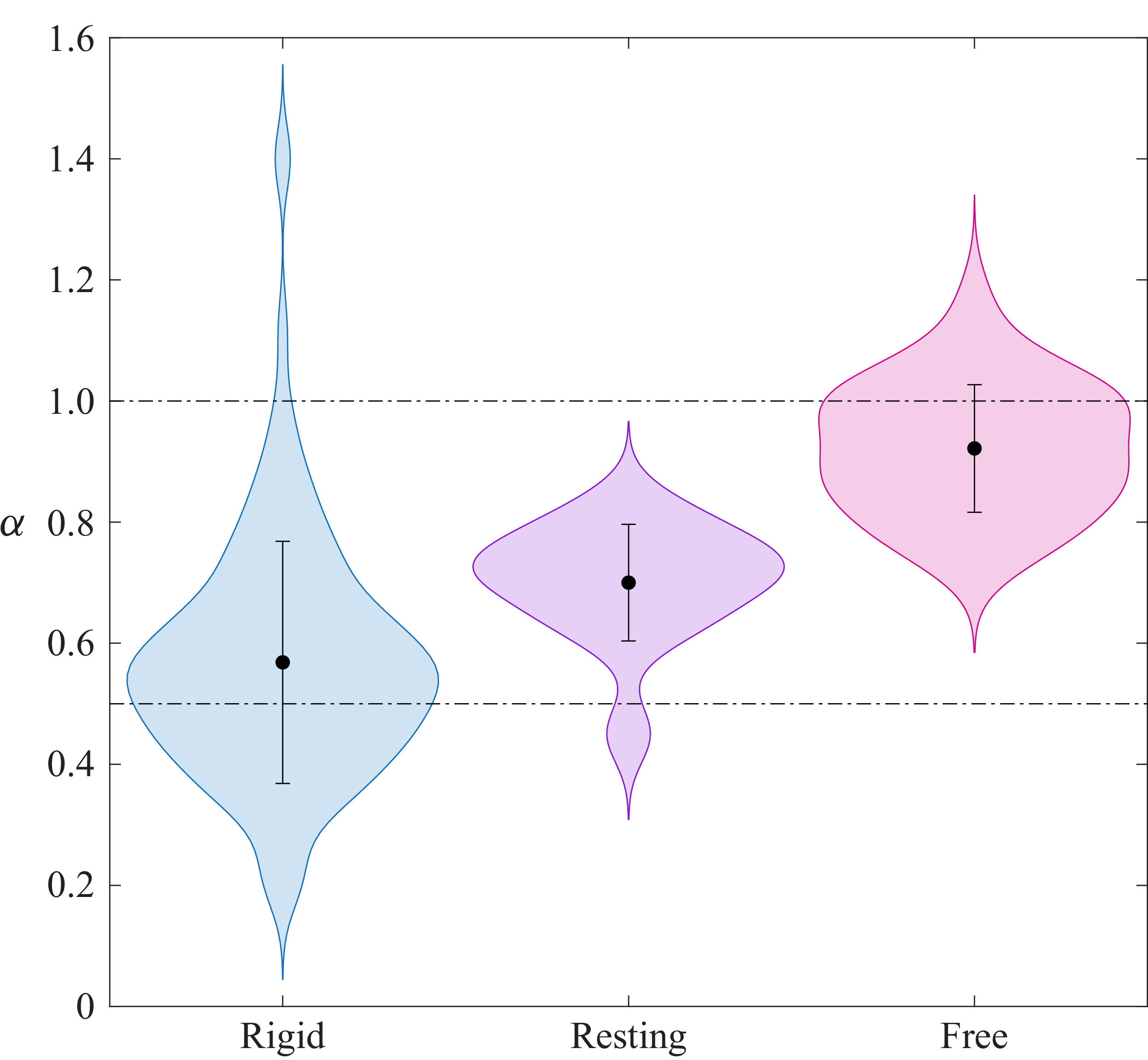
 α

 C=3.14
 C=3.21
 U
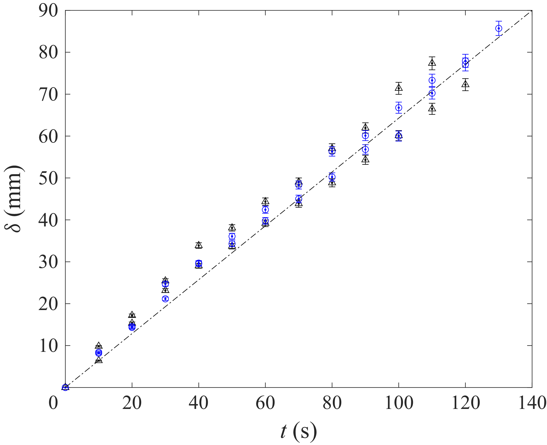
 C=6.35

 U
 C=6.35,6.15
 6.0
 U
 σS
 σS
 σ0
 σ0=27,17,11

 △
 ◃
 ◻
 σS
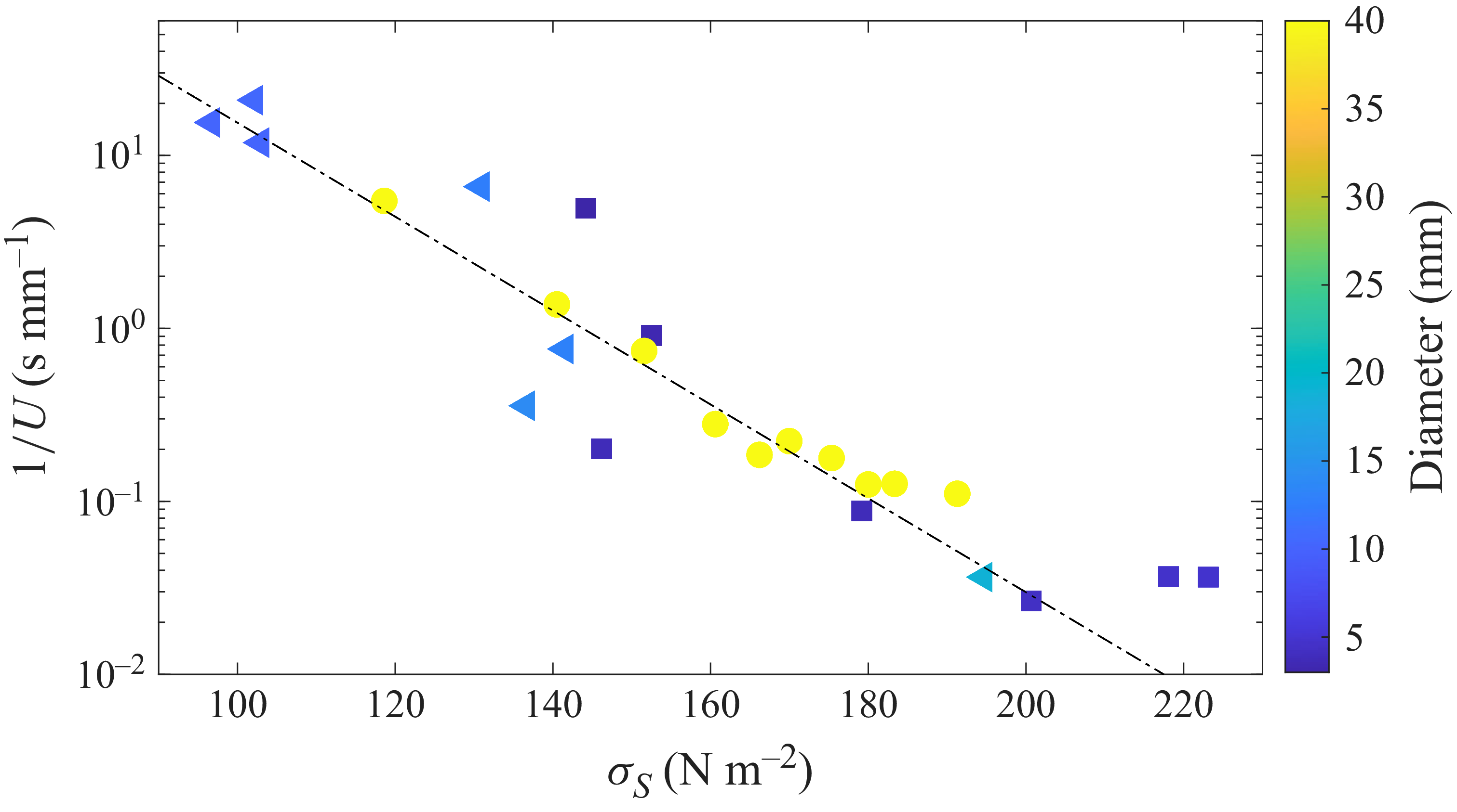
 ◃
 ◻
 ∘
 σ0=16

 U
 V
 |v|=V2+U2
 ∼1

 32
 10
 C=6.35

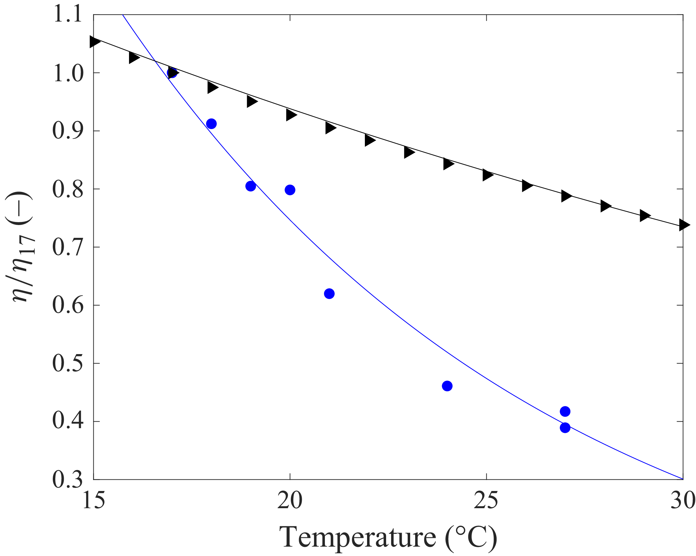
 C=6.35
 σS=213
 17
 ∘


 Open access

