

Introduction
Playing out against the backdrop of a long-standing disciplinary divide pitting idiographic history against nomothetic social science, the emergence of social science history was marked by a concerted effort to bring the tools of quantitative social science to bear on historical materials, with a particular emphasis on the study of political history. While the use of quantitative methods is now an established part of historical research in both history and the social sciences, the use of traditional forms of global regression remains a contested practice, even among quantitatively oriented scholars. A regression model can be said to be global to the extent that it assigns a single parameter to any given predictor, thereby assuming that the relationship between the outcome and the predictor is constant or homogeneous. Critics contend that the homogeneity assumption runs afoul of the basic tenets of historical analysis, which is fundamentally concerned with understanding how time and space inform the explanation of historically situated cases (see Tilly Reference Tilly1977, Reference Tilly1981, Reference Tilly1984). This attention to the effect of historical context is lost in conventional approaches to regression, producing results that are fundamentally ahistorical insofar as they assume a priori that the relationships being modeled are fixed across the set of observations.
With this problem in mind, quantitative researchers have come to link historical analysis to parameter heterogeneity, focusing in particular on the introduction of time-varying parameters in the analysis of time-series data (e.g., Isaac and Griffin Reference Isaac and Griffin1989; Wawro and Katznelson Reference Wawro and Katznelson2014; Western and Kleykamp Reference Western and Kleykamp2004). Drawing on recent innovations in spatial statistics, I show how this type of approach can be extended to the case of spatial data using a technique known as random effects eigenvector spatial filtering, which provides a fast, low-rank approximation of a Bayesian spatially varying coefficient model (Murakami et al. Reference Murakami, Takahiro Yoshida, Griffith and Yamagata2017). The benefits of this method are especially pronounced for the study of political history, where the adoption of quantitative methods went hand in hand with the use of spatial data. This article contributes to the literature on quantitative history and the study of politics by illustrating how spatially varying coefficient models can be used to help understand political history as a spatially situated process—a central concern in fields such as political and historical sociology, where questions of place and space have come to the fore in recent years (e.g., Sewell Reference Sewell2001; Tilly Reference Tilly2000).
Whereas existing work on the role of spatial effects in mass politics has typically focused on spatial dependence and local interaction in the diffusion of political contention (e.g., Andrews and Seguin Reference Andrews and Seguin2015; Gould Reference Gould1991; Tolnay et al. Reference Tolnay, Deane and Beck1996), I focus on the problem of spatial heterogeneity in the context of the Populist movement of the late nineteenth century, which saw farmers throughout the agrarian periphery turn to third-party candidates as a means of combating economic insecurity and exploitation resulting from their position in a rapidly expanding market for agricultural commodities such as wheat. Benefiting from the availability of aggregate voting data, studies of the electoral phase of the Populist movement played a central role in the evolution of the new political history movement (e.g., Argersinger Reference Argersinger1974; Cherny Reference Cherny1981; Hackney Reference Hackney1969; Parsons Reference Parsons1973; Wright Reference Wright1974). From this perspective, the emergence of electoral Populism can be understood as both a significant event in the trajectory of American politics, as well as a critical case in the development of quantitative history, and thus serves as a natural object of inquiry.
Drawing on county-level data from Kansas, Minnesota, Nebraska, North Dakota, and South Dakota, I use random effects eigenvector spatial filtering to capture the heterogeneous effects of variables representing economic and ethnocultural divides. Allowing the effects of these variables to differ across locales serves both a negative and positive function. On the one hand, the use of a spatially varying coefficient model protects against the types of false generalizations that result from an uncritical reliance on the conventional global model, which has the potential to misrepresent a local phenomenon as a general pattern. Such is the case when considering the effect of factors such as wheat dependence and the size of the ethnic German population on the degree of support for Populist candidates. On the other hand, the use of a spatially varying coefficient model lends itself to the construction of typological generalizations, allowing us to chart a middle route between nomothetic and idiographic explanation, as advocated in the growing literature on causal complexity in comparative-historical research (e.g., Ragin Reference Ragin1987, Reference Ragin2000). This is evident when using spatially varying coefficient models to examine patterns of third-party mobilization in the American West, where variation in the relationship between ethnic composition and third-party vote share contributed to the appearance of distinct varieties of electoral Populism.
Historical Analysis in the Quantitative Age
The relationship between history and the social sciences has always been somewhat uneasy. In spite of sharing common substantive interests, the two camps differ significantly in terms of their choice of methods and approach to explanation. The roots of this divide can be traced back to the Methodenstreit of the late nineteenth century, which famously pitted members of the German Historical School of Economics against their counterparts in the Austrian School. At the heart of the debate was a question about what kind of science economics should be. Whereas proponents of the German Historical School argued that economics should be an idiographic science focused on the explanation of historically situated events (i.e., events situated in time and space), proponents of the Austrian School argued that economics should be a nomothetic science oriented toward the construction of general laws. In the end, the latter view won out, as evidenced by the growing dominance of neoclassical economics. Once economists turned their collective attention to the laws of supply and demand, the study of economic history quickly faded into the background, having been left to historians as part of an emerging division of intellectual labor. This debate was by no means unique to economics, nor was this the last time that appeals to generality would be used to actively distinguish the practice of social science from the practice of history (e.g., Kiser and Hechter Reference Kiser and Hechter1991; Lipset Reference Lipset1968 Reference Lipset). The potential for renewed conflict was due in large part to the proliferation of quantitative methods in the social sciences during the post–World War II period. While the quantification of disciplines such as economics, political science, and sociology generally served to reinforce the divide between history and the social sciences, it also created opportunities for subversive innovation within fields (Abbott Reference Abbott1991; Calhoun Reference Calhoun1996; Robertson Reference Robertson1994). This is precisely what happened in the field of history in the 1960s and 1970s when political historians began adopting quantitative methods as a means of challenging the prevailing methodological orthodoxy within their home discipline. The result was the new political history movement, which eventually led to the formation of the Social Science History Association in 1974 (Bogue Reference Bogue1987). While quantitative history is here to stay as part of both history and the social sciences, the idea of using conventional quantitative methods to examine historical data is not without its critics. Many traditional historians saw the arrival of quantification as an expensive and inaccessible distraction that threatened to undermine the practice of narrative history in all its idiographic glory (see Ruggles Reference Ruggles2021 for a review). The more surprising response came from historically oriented social scientists who remained committed to the prospect of quantification yet took issue with how quantitative history was typically done. From this perspective, the solution was not to make history less quantitative, but to make conventional quantitative methods such as regression more historical. To the extent that historical analysis is characterized by attention to the effects of time and space, this means allowing for variation in the underlying data generating process. More specifically, this means moving away from standard approaches to regression, which assign one coefficient to each covariate as part of a single global model, thus destroying the contextual complexity that marks the unfolding of social life.
Global Regression and Its Discontents
Critics charge that the fundamental problem with quantitative history is not so much that it uses numbers, as it is that the uncritical reliance on global models tends to produce explanations that are divorced from the historical context in which those numbers were produced (see Isaac and Griffin Reference Isaac and Griffin1989; Wawro and Katznelson Reference Wawro and Katznelson2014). When a researcher says that quantitative history is historical what they usually mean is that the materials being examined are from the past. The key idea going forward is that the use of historical materials is a necessary but not sufficient condition for historical analysis. To paraphrase Charles Tilly (Reference Tilly1977, Reference Tilly1981, Reference Tilly1984), an analysis is only historical insofar as it is grounded in time and space, which together define the historical context in which actors are situated. This is not to deny the possibility of empirical generalization so much as it is to acknowledge that different processes may hold in different historical settings, dashing the researcher’s hopes for a conclusion that is both simple and general (Griffin Reference Griffin1992). What does this mean for the practice of quantitative history, where our findings are typically expressed in terms of a set of regression coefficients reflecting the extent to which a given set of covariates is associated with the outcome of interest? It means, among other things, allowing the parameters in question to vary across time and space (Abbott Reference Abbott1988).
The connection between historical analysis and parameter heterogeneity has been discussed at length in the literature on time and temporality in the social sciences. Isaac and Griffin (Reference Isaac and Griffin1989), for example, contend that conventional approaches for dealing with time-ordered data such as time-series regression and event history analysis are ahistorical insofar as they ignore temporal variation in the underlying parameters. To address this problem, they propose what they refer to as “moving covariance analysis”—a simplified version of the moving regression approach originally outlined by Brown et al. (Reference Brown, Durbin and Evans1975). Drawing on data on labor organization and conflict between 1882 and 1980, Isaac and Griffin show that the relationship between changes in strike frequency and factors such as union growth, union foundings, and union disbandings underwent a pronounced shift in the late 1930s. Under these conditions, the traditional global model is rendered useless, in the sense that it produces a conclusion that is simple but not general.
Variants of moving regression have been used to good effect to examine topics related to labor (e.g., McCammon Reference McCammon1993), social movements (e.g., Kane Reference Kane2007), voting (e.g., Lin Reference Lin1999), crime and punishment (e.g., King et al. Reference King, Massoglia and Uggen2012), culture (e.g., Pescosolido et al. Reference Pescosolido, Grauerholz and Milkie1997), and racial violence (e.g., Beck and Tolnay Reference Beck and Tolnay1990). Whereas moving regression produces alternative estimates by systematically rerunning the same model on different subsets of data, recent approaches have eschewed brute force computation in favor of more complex models in which temporal variation in the parameter estimates is modeled directly. This is particularly true in the field of political science, where the introduction of new methods for modeling discrete change points (e.g., Hermansen et al. Reference Hermansen, Henrik Knutsen and Mokleiv Nygård2021) and time-varying parameters (e.g., Wood Reference Wood2000) has become something of a cottage industry. The proliferation of techniques designed to capture temporal heterogeneity is due in no small part to the growing popularity of Bayesian methods, which offer considerable flexibility over more conventional alternatives (e.g., Wawro and Katznelson Reference Wawro and Katznelson2014; Western and Kleykamp Reference Western and Kleykamp2004).
As the preceding discussion suggests, efforts to make quantitative history more historical have focused overwhelmingly on the use of time-varying parameters. Yet historical analysis is as much about space as it is about time. The goal of this article is to show how the idea of parameter heterogeneity can be extended to the case of space using random effects eigenvector spatial filtering. This is done with an eye toward political history, where the use of spatial data is especially common among quantitative researchers, who have long relied on election returns as a means of capturing variation in political sentiment across locales. Prior to the survey revolution, data on precincts, counties, and other such areal units were often all that were available. In this respect, the earliest studies of political behavior were necessarily oriented around questions regarding the spatial organization of mass politics (e.g., Gosnell Reference Gosnell1937; Key Reference Key1949). Given the paucity of individual-level data with which to work, it is not surprising that the use of aggregate election data became a hallmark of the new political history movement, which took the emergence of electoral Populism in the United States during the late nineteenth century as one of its central cases.
Revisiting the example of electoral Populism thus has the potential to shed new light on the case, as well as the more general challenges associated with the practice of quantitative history and the study of political contention. This is true in two interrelated respects. First, while a significant amount of attention has been paid to the diffusion of political contention across locales (e.g., Andrews and Seguin Reference Andrews and Seguin2015; Gould Reference Gould1991; Tolnay et al. Reference Tolnay, Deane and Beck1996), far less has been said about the role of spatial heterogeneity in historical settings. To the extent that it has been considered (e.g., Darmofal Reference Darmofal2008), researchers have tended to rely on techniques such as classical geographically weighted regression, which is known to be problematic (Wheeler and Calder Reference Wheeler and Calder2007). Second, allowing for spatial heterogeneity speaks to a growing interest in causal complexity in comparative-historical research, where researchers have increasingly pushed back on the tendency to assign a single effect to each predictor (e.g., Ragin Reference Ragin1987, Reference Ragin2000). This leads to the possibility of typological generalizations representing the variety of ways in which the outcome of interest is connected to the characteristics of the concrete observations at hand.
The Populist Movement Revisited
The Populist movement was the culmination of an ongoing struggle to combat the side effects of economic development in the wake of the Civil War. Responding to the vagaries of an economic system dominated by banks, railroads, and other market intermediaries, farmers throughout the agrarian periphery turned to collective action, flocking to groups such as the Farmers’ Alliance, which served as the organizational backbone of the emerging movement. Though not wholly apolitical, the Alliance was initially oriented toward economic cooperation, with ambitious cooperative experiments emerging independently in both the South and West. These projects proved difficult to sustain in the absence of concerted regulation. Stymied by the constraints of a market in which organized collusion was a norm, the Alliance was quickly drawn into politics as a means of pursuing its economic goals. As economic cooperation gave way to political mobilization, Alliance leaders were faced with the following question: Should they work within the existing party system or form a new party of their own? The prospects for an independent party were extremely limited in the South, where the Democratic Party served as a vehicle for racial domination. So, while Populists in the South and West shared a common interest in economic cooperation, it was western Populists who led the charge into the electoral arena in 1890.
Motivated by the success of independent candidates in states such as Kansas, Minnesota, Nebraska, and South Dakota, western Alliance leaders were quick to advocate for the creation of a new national party. When the People’s Party finally held its first nominating convention in the summer of 1892, it put forward a platform calling for government control of currency; a commitment to free silver; the establishment of postal savings banks; public ownership of railroads, telegraphs, and telephones; and a prohibition on alien landownership. In practice, the fact that the Populist movement had a party of its own did little to resolve the question whether to collaborate with one of the major parties. Supporters of the third-party movement were consistently divided over the practice of cross-endorsement, which allowed so-called fusion candidates to run under more than one party label, thus allowing third-party candidates to garner major party support while maintaining an independent platform. The growing divide between the pro- and antifusion factions reached its breaking point in the run-up to the election of 1896, when the fusionists finally won out with the nomination of presidential candidate William Jennings Bryan, who ran as both a Populist and a Democrat.
The push for electoral fusion went hand in hand with the fight for free silver, which quickly became the defining issue of the Bryan campaign. Strategically, the appeal of free silver lay in its ability to attract not only Populists and Democrats but Republicans as well. In the end, Bryan managed to secure nearly 47 percent of the popular vote—a significant showing for a Populist candidate, though well below what was required to win what was, for all intents and purposes, a two-party race dominated by an ascendant Republican Party. Irreparably torn over the twin issues of fusionism and free silver, the People’s Party more or less disintegrated in the wake of Bryan’s defeat, taking the Populist movement with it. While the party continued to run candidates for several years, it ceased to be a viable entity after 1896.
Electoral Populism and the Rise of Social Science History
Discussions of Populist mobilization have tended to follow the intellectual trajectory of American historiography more generally, starting with the emergence of the Progressive school in the early twentieth century. From the perspective of Progressive historians such as Hicks (Reference Hicks1931), the emergence of the Populist movement was a rational response to economic hardship. This view began to change in the 1950s when a surge in popular support for totalitarian rule under Wisconsin Senator Joseph McCarthy prompted researchers to reinterpret the rise of agrarian radicalism in the nineteenth century as a retrogressive movement bordering on protofascism (see Bell Reference Bell1955; Ferkiss Reference Ferkiss1957). The predominant tendency among these postwar revisionists, known as the consensus school, was to substitute ostensibly psychological concepts such as status anxiety for economic interest as a means of suggesting that the Populist movement was somehow fundamentally irrational, insofar as it opposed the institutionalization of industrial capitalism in the United States. This style of thinking is most closely associated with the work of Hofstadter (Reference Hofstadter1955), who argued that Populist sentiment was a product of conflicting identities borne out of the tension between commercial agriculture and the cultural legacy of the yeoman tradition that it replaced.
The consensus approach to Populism was, however, quickly swept aside following a number of high-profile critiques (e.g., Nugent Reference Nugent1963; Pollack Reference Pollack1962; Rogin Reference Rogin1967), eventually giving way to the wave of “new” histories that began to flood the field in the 1960s. In this context, traditional economic accounts were not so much defended as they were reborn under the auspices of New Left history and new social history, which came together most clearly in Lawrence Goodwyn’s Democratic Promise (Reference Goodwyn1976). Anticipating innovations in the study of social movements more generally, Goodwyn argued that the politicization of the Populist movement was an outgrowth of a movement culture fostered by experiments in economic cooperation under the Farmers’ Alliance (cf. Parsons et al. Reference Parsons, Toombs Parsons, Killilae and Borgers1983), ushering in a stream of studies examining the organizational foundations of collective identity and mass mobilization during the Populist moment (e.g., Barnes Reference Barnes1984, Reference Barnes2011; Gerteis Reference Gerteis2007; McNall Reference McNall1988; Schwartz Reference Schwartz1976). The study of Populism was similarly influenced by the introduction of quantitative methods as part of the push for what became known as new political history. Inspired by the work of sociologist Paul Lazarsfeld and his collaborators at the Bureau of Applied Social Research, these quantitatively oriented researchers attempted to understand the emergence of electoral Populism in terms of the social cleavages underlying the party system, which were not solely economic in nature (see Bogue Reference Bogue1990).
In the nineteenth century, party allegiances were closely tied to lines of ethnocultural conflict, with issues such as the establishment of parochial schools and, perhaps more importantly, the enforcement of prohibition becoming important points of political contention (Jensen Reference Jensen1971; Kleppner Reference Kleppner1970; Luebke Reference Luebke1977). Armed with ecological data in the form of election returns and census counts, quantitatively oriented historians could now formally adjudicate between economic theories of electoral Populism, on the one hand, and ethnocultural theories, on the other (e.g., Argersinger Reference Argersinger1974; Cherny Reference Cherny1981; Parsons Reference Parsons1973; Wright Reference Wright1974). These debates were integral to the development of quantitative history as a recognized subfield. At the same time, the tools that the new political historians had readily available to them were fairly rudimentary, ranging from bivariate correlation to stepwise regression, neither of which accounts for heterogeneity in the data generating process. While the tools used to study electoral Populism have improved considerably (e.g., Smångs and Redding Reference Smångs and Redding2019), research on this front remains relatively untouched by work in the field of spatial statistics, including recent innovations in the treatment of spatial heterogeneity.
This is not to say that existing work has ignored the problem of spatial context altogether. Indeed, the best known quantitative accounts of electoral Populism introduce statistical analysis as part of a more traditional historical case study, typically focusing on a single state (e.g., Argersinger Reference Argersinger1974; Cherny Reference Cherny1981; Hackney Reference Hackney1969; Parsons Reference Parsons1973; Wright Reference Wright1974). In this respect, existing work on this front is deeply attentive to the effect of local conditions on the origins of agrarian radicalism. That having been said, the statistical estimates that these studies produced were unambiguously global, in the sense that they applied to each study area as a whole, with researchers paying little attention to how effects varied within or between study areas. This raises the question whether the association between electoral Populism and factors such as economic hardship and ethnic composition was similar across locales. Ostler (Reference Ostler1993) implicitly points in this direction, using qualitative comparison to show how variation in state party systems contributed to differences in the effect of economic conditions on third-party mobilization, focusing in particular on the contrast between western Iowa, on the one hand, and eastern Kansas and Nebraska, on the other. Though the two regions were economically similar, Populist candidates fared far better in Kansas and Nebraska than they did in Iowa. Extending this logic to the quantitative domain, models of spatial heterogeneity explicitly formalize the interaction between covariates and locales, producing a unique topography of effects for each predictor, allowing us to systematically compare the differences in the correlates of electoral Populism from one place to the next.
Data
The following analysis uses county-level voting and census data to examine the spatial dynamics of electoral Populism in Kansas, Minnesota, Nebraska, North Dakota, and South Dakota in the period between 1890 and 1896. Together, these five states make up the western wheat belt where the third-party movement first emerged (Hicks Reference Hicks1931). In a small number of cases, county boundaries changed over the course of the study period. Following Bailey and Snedker (Reference Bailey and Snedker2011), Gullickson (Reference Gullickson2010), and Tolnay et al. (Reference Tolnay, Deane and Beck1996) among others, unstable counties were combined to create geographically stable clusters.Footnote 1 Analysis is limited to counties and county clusters that were fully settled by 1890, meaning that they not only had an enumerated population but recorded votes in the 1890 election as well.
Dependent Variable
In a stable two-party system, it is easy to take for granted that party labels mean the same thing across time and space. This was not the case, however, in the late nineteenth century when parties routinely relied on electoral fusion or cross-endorsement to help their chances at the polls. In the West, Populist candidates were periodically endorsed by the Democratic Party, allowing them to run as independent or third-party candidates while still picking up major-party support. The situation was further complicated by the fact that fusion could be effected at the state or district level, meaning that the same candidate could be endorsed differently from one place to the next, as was the case with the presidential election of 1892, which saw Populist James B. Weaver run as an independent candidate in some states (e.g., Minnesota, Nebraska, and South Dakota) and a fusion candidate in others (e.g., Kansas and North Dakota). The presidential election of 1896 is the only race in which voters in the study region would have seen the same similarly endorsed candidate. The election of 1896 was unique in the extent to which it focused on monetary policy and the debate over free silver—an issue that could be used to leverage an endorsement from the Democratic Party. The adoption of single-issue fusion may have increased Populist vote share, but it also contributed to the demise of the party by creating an irreparable divide within the movement from which it sprang.
The example of 1896 highlights a more general problem, namely that there was no such thing as a representative race in a moment of radical institutional flux in which changes in the political environment far outpaced changes in the underlying conditions that gave rise to electoral Populism in the first place. I address this problem by combining data from multiple races. More specifically, I examine between-county variation in the average vote share received by Populist-backed candidates in gubernatorial races between 1890 and 1896 using time-invariant covariates measured at the start of the study period. Voting data were drawn from the United States Historical Election Returns, 1824–1968 dataset (Inter-University Consortium for Political and Social Research 1999). The advantage of focusing on gubernatorial contests is twofold. Not only were elections held every two years in Kansas, Minnesota, Nebraska, North Dakota, and South Dakota but also each race between 1890 and 1896 featured a Populist-backed candidate. The governorship was the only major office for which this was the case.
Independent Variables
Debates over the foundations of partisanship in the late nineteenth century generally boil down to a question of economics versus culture. The emergence of electoral Populism has traditionally been linked to wheat-producing regions where a lack of diversified agricultural effectively locked settlers into an already precarious market. Though some question whether this relationship holds in practice (e.g., Argersinger Reference Argersinger1974; Ostler Reference Ostler1993), the wheat-belt hypothesis remains a standard point of reference, figuring heavily in classic accounts (e.g., Hays Reference Hays1957; Hofstadter Reference Hofstadter1955; Lipset Reference Lipset1950), as well as in more contemporary work (e.g., Sanders Reference Sanders1999). For the purpose of the following analysis, wheat dependence is measured in terms of the percent of improved acreage devoted to the production of wheat in 1890. I anticipate that the level of support for Populist candidates will be positively associated with the level of wheat dependence, all else being equal. Crop choice was, of course, not the only factor affecting the economic livelihood of agrarian producers. Mortgages were perhaps the most pressing source of debt in the West and are frequently cited when recounting the standard Populist grievances (e.g., Hicks Reference Hicks1931). With this issue in mind, I control for the percentage of farm families that were classified as encumbered owners (as opposed to free owners or renters). The expectation is that, net of other factors, levels of Populist support should be positively associated with the prevalence of farm mortgages.
The politicization of economic issues during this period played out against the backdrop of existing cultural divides bound up in patterns of ethnic and religious identification. While the exact configuration of ethnic blocs varied from state to state, the German and Scandinavian populations stand out in particular. I thus control for (1) the percentage of the total population that was born in either Germany or Russia, as well as (2) the percentage of the population that was born in either Sweden, Norway, or Denmark. Whereas the German community tended to be staunchly anti-Populist on account of the movement’s affinity toward temperance and suffrage, Scandinavian voters had fewer cultural qualms with the Populist program and were thus more willing to back third-party upstarts. In an effort to facilitate the graphical representation of results, the percent German variable was reverse coded prior to analysis to ensure that the corresponding coefficient would run in the same direction as the other coefficients of interest. In practice, this means controlling for the size of the non-German population. Though the decision to count Russian-born settlers as part of the German population may seem surprising, the vast majority of Russian settlers in the study area were from German-speaking regions of Russia and tended to identify as German. It is important to note that reverse coding has no effect on the magnitude of the resulting coefficients. As such, coefficients associated with the size of the non-German population can be flipped to produce equivalent statements about the relationship between the size of the German population and average third-party vote share.
The preceding measures were constructed using county-level census data contained in the Historical, Demographic, Economic, and Social Data: The United States, 1790–2000 dataset (Haines and the Inter-University Consortium for Political and Social Research Reference Haines2005). For the purposes of visualization, these measures were rescaled to have a mean of 0 and a standard deviation of 0.5 (see Gelman Reference Gelman2008). In addition to the independent variables just described, I also control for state membership. In the absence of political and economic centralization, state governments in the United States were arguably the primary point of reference when it came to political mobilization. Indeed, prior to the start of the New Deal in the 1930s, the party system in the United States was highly localized. More often than not, political elites continued to ally with a major party, though what these party labels stood for tended to vary from one place to the next (see Chhibber and Kollman Reference Chhibber and Kollman2004: 208–20). This was particularly true in the American West where states such as North Dakota and South Dakota were only just beginning to make the transition from the “chaotic factionalism” of the territorial period (Owens Reference Owens1970). To the extent that the opportunities afforded by the party system varied from one state to the next, average Populist vote share is expected to vary as well (see Ostler Reference Ostler1993). These types of standing differences between states were further compounded by short-run differences in the prevalence of electoral fusion in gubernatorial races, which added major-party votes to the Populist total.
Methods
Whereas traditional quantitative accounts of electoral history assume that each independent variable produces a single effect in a given study area, the following analysis allows for continuous spatial heterogeneity in the form of a spatially varying coefficient model. As the name suggests, the idea behind a spatially varying coefficient model is to let the value of one or more coefficients vary across a set of spatially situated observations, thus highlighting the effect of geographic context on the process at hand. The problem with estimating a separate set of parameters for each observation is that the number of parameters to be estimated quickly outruns the number of observations. One way around this is to use a Bayesian spatially varying coefficient (BSVC) model, which treats the set of unit-specific estimates as draws from a multivariate normal distribution (see Gelfand et al. Reference Gelfand, Kim, Sirmans and Banerjee2003). Simulation studies confirm that BSVC models avoid a number of the problems associated with popular alternatives such as classical geographically weighted regression (Wheeler and Calder Reference Wheeler and Calder2007), though not without some computational cost (Finley Reference Finley2011). Recent work shows, however, that random effects eigenvector spatial filtering can be used to construct a fast, low-rank approximation of a BSVC model (Murakami et al. Reference Murakami, Takahiro Yoshida, Griffith and Yamagata2017), thus bypassing many of the hurdles that accompany more traditional approaches.
Random Effects Eigenvector Spatial Filtering Models
The basic idea behind eigenvector spatial filtering (ESF) is that eigen decomposition—a standard algebraic operation—can be used to translate a set of spatial relationships into a series of observable covariates. Like ESF models more generally, the random effects eigenvector spatial filtering (RE-ESF) model builds on the Moran coefficient or Moran’s I, a popular measure of spatial autocorrelation. The formula for Moran’s I can be expressed in matrix form as follows:
 $$I = {n \over {{\bf{1}^ \top }{\bf{C}}\bf{1}}}{{{{\bf{y}}^ \top }{\bf{MCMy}}} \over {{{\bf{y}}^ \top }{\bf{My}}}},$$
where 1 refers to an n × 1 vector of ones, and y refers to an n × 1 vector of outcomes. The key to ESF is the doubly centered connectivity matrix MCM, which is based on the set of uncentered connectivities given by C—an n × n matrix used to represent the spatial relationship between observations. To the extent that RE-ESF models are used to approximate BSVC models, the relationships in question are typically expressed in terms of distance. Using an exponential function, for example, the value of cii′ is given by cii′ = exp(−dii′/h) for i≠i ′ and 0 otherwise, where dii′ refers to the distance between observations i and i ′, while h refers to the maximum nearest-neighbor distance across all ii ′ pairs. The centering matrix M is defined as I – 11┬/n, where I refers to an n × n identity matrix.
For the purposes of ESF, the matrix MCM is decomposed into a matrix of eigenvectors E and a diagonal matrix of eigenvalues Λ, such that MCM = EΛE┬. In this framework, each n × 1 eigenvector in E is paired with an eigenvalue. The eigenvalues in question are arrayed along the diagonal of Λ, ordered from largest to smallest. Taking a subset of the eigenvectors of MCM, we can construct an orthogonal basis function representing the autocorrelation process underlying the spatial distribution of coefficients. In practice, it is common to work with the n × q submatrix of eigenvectors
 ${\bf{\tilde E}}$
associated with the q × q submatrix of positive eigenvalues
 ${\bf{\tilde \Lambda }}$
, which is equivalent to assuming positive spatial autocorrelation. Each eigenvector
 ${{\bf{\tilde e}}_m}$
in
 $m = 1, \ldots ,q$
produces a unique map pattern; the value of the corresponding eigenvalues are directly proportional to the value of the Moran coefficients associated with the map patterns in question (Murakami et al. Reference Murakami, Binbin Lu, Chris Brunsdon, Nakaya and Griffith2019). Substantively speaking, this means that the observed map patterns become increasingly localized as we move from
 ${{\bf{\tilde e}}_1}$
to
 ${{\bf{\tilde e}}_q}$
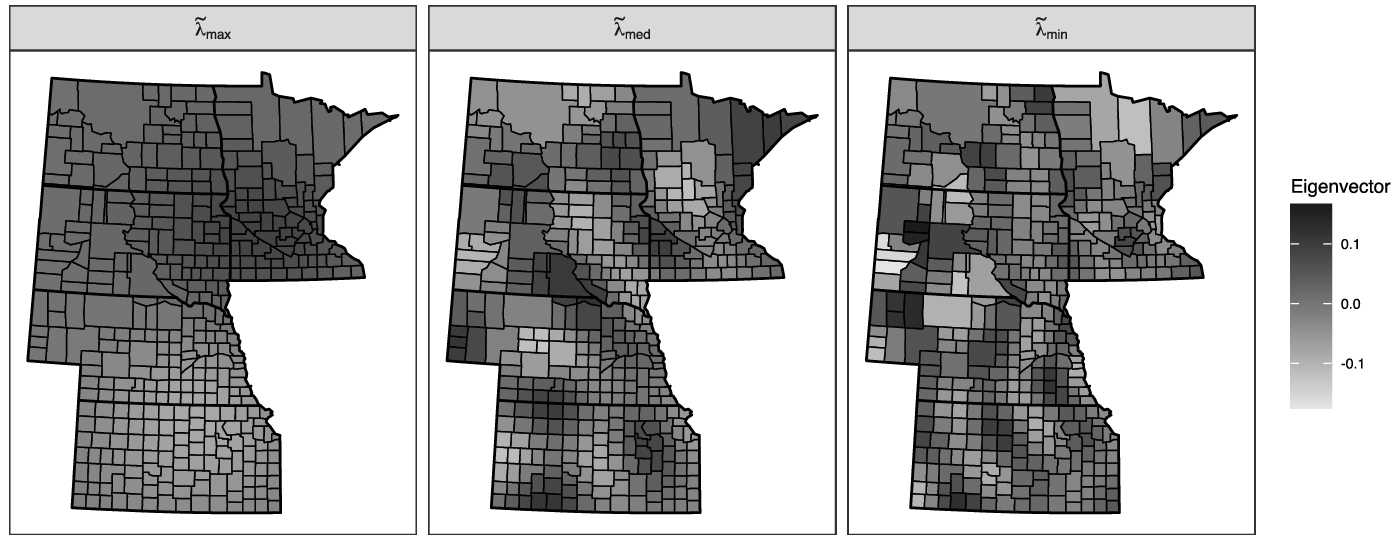
. This is evident in figure 1, which depicts the orthogonal map patterns corresponding to the maximum, median, and minimum positive eigenvalues for counties in Kansas, Minnesota, Nebraska, North Dakota, and South Dakota, which collectively constitute the study area in the analysis below.Footnote 2 As we move from maximum to minimum, we find that observations tend to look less and less like their neighbors, as reflected in the value of the Moran coefficient, which drops from 0.9365 at the maximum to 0.0518 at the median, eventually falling to 0.0001 at the minimum, at which point the spatial distribution of values is near-random.
Map of select eigenvectors for Kansas, Minnesota, Nebraska, North Dakota, and South Dakota.

RE-ESF models build on the idea that the matrix of positive eigenvectors can be treated as a set of observable covariates. The resulting model can be written as
 $$\matrix{ \hfill {\bf{y}} {\ = \mathop \sum \limits_k {{\bf{x}}_k} \circ {{\bf{\beta }}_k} + {\bf{\varepsilon }},{\bf{\varepsilon }} \sim N\left( {{{\bf 0}_{1 \times n}},\sigma _\varepsilon ^2{\bf{I}}} \right),} \cr \hfill {\bf{\beta}}_k {\ = {{\tilde \beta }_k}{\bf{1}} + {\bf{\tilde E}}{{\bf{\gamma }}_k},{{\bf{\gamma }}_k} \sim N\left( {{{\bf 0}_{1 \times q}},\sigma _{{\gamma _k}}^2{{{\bf{\Lambda }}}_k}} \right),} \cr } $$
where
 ${{\bf{x}}_k}$
refers to an
 $n \times 1$
vector depicting the values of the
 $k$
th covariate in
 $k = 1, \ldots ,p$
, while
 ${\bf{\beta }}_k$
refers to an
 $n \times 1$
vector of unit-specific coefficients, with
 ${\bf{x}}_k \circ {\bf{\beta}}_k$
representing the elementwise product of the two. As the preceding formula suggests, we are, in effect, decomposing the vector of local coefficients
 ${\bf{\beta}}_k$
in terms of a constant aspatial component
 $\tilde\beta_k\bf{1}$
and a spatially varying component
 ${\bf{\tilde E}}{{\bf{\gamma }}_k}$
. What sets the RE-ESF model apart from a conventional ESF model is that the coefficients making up
 ${\bf{\gamma}}_k$
are treated as draws from a common distribution. We assume in particular that the
 $q \times 1$
vector of coefficients
 ${\bf{\gamma}}_k$
is drawn from a
 $q$
-dimensional multivariate normal distribution with a mean vector of zero and a variance-covariance matrix given by
 ${\sigma _{{\gamma _k}}^2{{\bf{\Lambda }}_k}} $
. Whereas
 $\sigma _{{\gamma _k}}^2$
denotes a shared variance parameter,
 ${{\bf{\Lambda }}_k}$
represents a
 $q \times q$
diagonal matrix, with the set of diagonal entries given by
 $\left(\sum_m \tilde{\lambda}_m / \sum_m\tilde{\lambda}^{\alpha_k}_m\right)\tilde{\lambda}^{\alpha_k}_m$
for
 $m = 1, \ldots ,q$
. This implies a heteroskedastic error structure in which the variance associated with the
 $m$
th coefficient
 $\gamma_{mk}$
is directly proportional to
 $\tilde{\lambda}^{\alpha_k}_m$
. Within this framework, the
 $\alpha_k$
term serves as a range parameter. More specifically, as the value of
 $\alpha_k$
increases, the coefficients associated with the nonleading eigenvectors are shrunk toward zero, limiting their influence on
 ${\bf{\beta}}_k$
, thus increasing the scale at which the set of unit-specific parameter estimates varies for any given covariate
 ${{\bf{x}}_k}$
. The set of local parameter estimates
 ${\bf{\beta}}_k$
are analogous to the random, unit-specific parameter estimates from a conventional multilevel model, with the average local effect given by the fixed effect
 $\tilde\beta_k$
.
Model Specification
By setting the variance parameter
 $\sigma _{{\gamma _k}}^2$
to zero for any given set of coefficients in
 ${\bf{\beta}}_1, \ldots , {\bf{\beta}}_p$
, we can incorporate both fixed and varying coefficients as part of the same model. The RE-ESF model reduces to a conventional global model when
 $\sigma _{{\gamma _k}}^2 = 0\forall k$
, allowing us to compare the global model to a range of more complex alternatives. In the following analysis, I begin by comparing the estimates produced using a conventional global model to the distribution of county-specific parameter estimates produced using an RE-ESF model in which the effect of each predictor is allowed to vary across counties. The only exceptions are the effects associated with the state dummy variables, which are meant to capture large-scale differences in the political environment between states, including differences in the propensity for electoral fusion, which inevitably inflated average Populist vote share across the period in question. The central question is whether the seemingly general conclusions produced using a global model can be reasonably supported by the data in front of us.
I take up this problem in the second part of the analysis, which uses measures of model fit to compare specifications, as well as to construct a composite representation of the resulting estimates. In this context, the purpose of introducing spatially varying coefficients is not to capture every last detail of the data generating process, but to account for the types of large-scale variation that systematically undermine the empirical validity of the global model. This has important implications for how we approach the question of model specification. The RE-ESF model can be estimated by maximizing the likelihood of the data, which serves as a natural metric for measuring the correspondence between the model in front of us and the data to which it was fit. When it comes to choosing one model over another, the problem is that the likelihood of the data can only increase in the face of more complex specifications. In other words, if we use the observed likelihood to compare models, we will always prefer the more complex specification.
The solution is to use a measure of fit that explicitly penalizes for complexity, thus allowing us to balance the demand for historical accuracy with the desire for explanatory parsimony. Popular options include the Akaike Information Criterion (AIC) and the Bayesian Information Criterion (BIC), both of which build off the observed likelihood in a straightforward way. In both cases, the magnitude of the penalty is a function of the complexity of the model, as measured by the degrees of freedom associated with the model in question.Footnote 3 For any given model j, the AIC value is defined as AICj = −2log(Lj) + 2dfj, where Lj refers to the corresponding likelihood, with the model degrees of freedom given by dfj. The BIC value is similarly defined as BICj = −2log(Lj) + log(n)dfj, where n refers to the sample size, with all other terms defined as before. To account for the fact that the number of parameters in the full RE-ESF model is relatively large compared to the number of observations, I use a small-sample variant of the AIC known as the AICc. For any given model j, the AICc value is given by
 ${\rm{AI}}{{\rm{C}}_{{c_j}}} = {\rm{AI}}{{\rm{C}}_j} + \left[ {\left( {2df_j^2 + 2d{f_j}} \right)/\left( {n - d{f_j} - 1} \right)} \right]$
.
Unlike a likelihood ratio test, the AICc and BIC can be used to compare both nested and nonnested models. When using the AICc or BIC to choose between models, we prefer the model with the lower value on whichever measure we are using. Whether this happens to be the more complex model depends on whether the increase in likelihood exceeds the penalty imposed by a given measure. Given the number of observations at hand and size of the models being considered, the BIC will tend to be more conservative than the AICc in this particular case, meaning that the BIC will tend to favor simpler models. In general, the amount of evidence in favor of the preferred model is reflected in the difference in the values used to compare the models in question. This holds for both the AICc and the BIC. Differences of two or more are generally seen as providing positive support in favor of the preferred specification, while differences of 10 or more are said to constitute very strong support in favor of the preferred specification (Raftery Reference Raftery1995; cf. Burnham and Anderson Reference Burnham and Anderson2002: 70–71).
In the analysis that follows, differences in the specification of the RE-ESF model are driven by choices regarding which sets of coefficients are allowed to vary. While the effects associated with the state dummy variables are treated as fixed in every model, the intercept is allowed to vary throughout, which serves as a correction for spatial dependence (Tiefelsdorf and Griffith Reference Tiefelsdorf and Griffith2007). Considering all possible combinations of fixed and varying coefficients across the remaining covariates results in 24 = 16 possible models, plus the global model from which we began. Rather than selecting the best fitting model, I use model averaging to combine local parameter estimates across models, with greater weight going to estimates from better-fitting models (Burnham and Anderson Reference Burnham and Anderson2002). To the extent that they are supported by the data, the inclusion of models with constant effects productively tempers the degree of variation across the set of local model-averaged parameter estimates associated with a given predictor. I use these estimates to produce a composite representation of the varieties of electoral Populism underlying the distribution of third-party support.
The relative influence of any given specification is reflected in the weights used to combine estimates. Using AICc values, for example, the weight assigned to model j is commonly given by
 $${{\rm{\omega }}_j} = {{\exp \left( { - 0.5 \times {\rm{\Delta AI}}{{\rm{C}}_{{c_j}}}} \right)} \over {\mathop \sum \nolimits_j \exp \left( { - 0.5 \times {\rm{\Delta AI}}{{\rm{C}}_{{c_j}}}} \right)}},$$
where
 ${\rm{\Delta AI}}{{\rm{C}}_{{c_j}}} = {\rm{AI}}{{\rm{C}}_{{c_j}}} - {\rm{AI}}{{\rm{C}}_{{c_{min}}}}$
refers to the difference between the AICc value associated with model j and the AICc value associated with the best-fitting model in the set, as denoted by
 ${\rm{AI}}{{\rm{C}}_{{c_{min}}}}$
. By construction, the value of ωj ranges between zero and one for any given model. This value represents the share of the total penalized likelihood associated with the model in question. The higher the value of ωj, the more model j contributes to the model-averaged estimate. For any given pair of models, there is a direct correspondence between the ratio of their respective weights and the difference in their respective
 ${\rm{\Delta AI}}{{\rm{C}}_{{c_j}}}$
values. This also holds for BIC weights, which can be constructed in a similar fashion.
Results
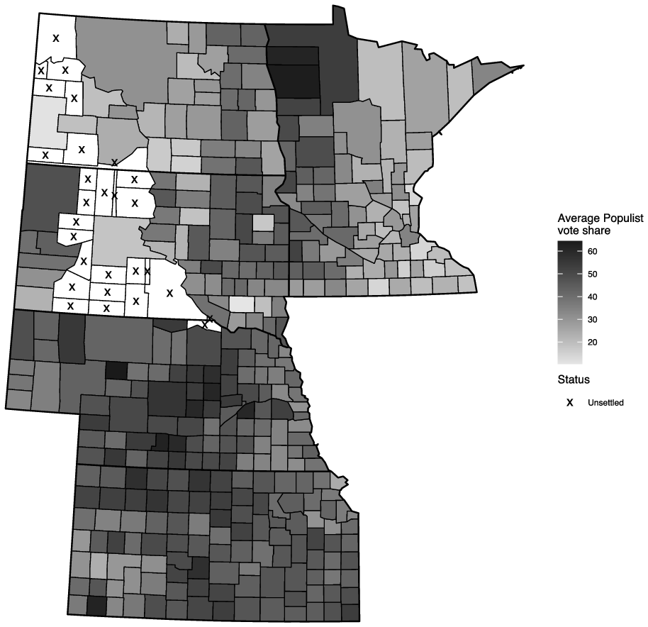
As can be seen in figure 2, average Populist vote share in settled counties varied widely across the region, ranging from a low of just under 11 percent in Hutchinson County, South Dakota to a high of more than 64 percent in Hooker County, Nebraska. In general, third-party candidates tended to fare best in Kansas and Nebraska. This was due in part to the effect of electoral fusion, a strategy first adopted by Kansas Populists in 1892 and Nebraska Populists in 1894. In contrast, Populists in Minnesota and South Dakota only sought cross-endorsement in 1896, at which point Democrat-Populist fusion was adopted nationwide. Fusion alone was not enough to guarantee support. In fact, electoral fusion had the potential to hurt candidates, as North Dakota Populists found out the hard way in 1890 when they made the unfortunate choice of deciding to join forces with the prohibition movement, costing themselves a fair amount of support at the polls. Even with the help of Democratic endorsements in 1892 and 1896, the rate of third-party voting in North Dakota continued to lag behind that of the other states in the region.
Average Populist vote share in settled in counties.

Comparing Global and Local Parameter Estimates
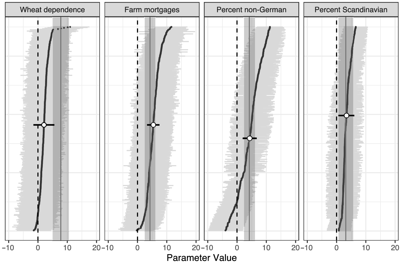
Using a global regression model, we can estimate the effect of factors such as wheat dependence, mortgage prevalence, and ethnic composition on the average share of the popular vote received by third-party candidates between 1890 and 1896, net of any between-state differences resulting from variation in the standing opportunities afforded by the local party system and/or the prevalence of electoral fusion over the course of the Populist moment. The question is whether the single set of effects produced by this model is a reasonable approximation of the underlying data generating process. To answer this question, we can compare the results produced using conventional linear regression to the results produced using a spatially varying coefficient model, which allows us to observe the heterogeneity that is intentionally suppressed by the standard global model, while also correcting for spatial dependence resulting from the connection between proximate units. Toward this end, figure 3 depicts the relationship between the estimates produced by the global model and the set of county-specific estimates produced using a RE-ESF model in which all of the effects are allowed to vary, with the exception of the effects associated with the state dummies (not reported).
Distribution of local parameter estimates by variable. The average local effect appears in white, along with the corresponding 95 percent confidence interval. Shaded areas refer to the 95 percent confidence interval from the global model.

For any given variable, the point estimate from the global model is represented by the vertical gray line, with the bounds of the 95 percent confidence interval represented by the bounds of the transparent gray region that surrounds it. The results of the global model are generally in line with what we would expect, in the sense that we observe significant positive effects for each of the covariates. Consistent with the wheat-belt hypothesis, we find that a two-standard deviation increase in the percentage of improved farmland devoted to wheat is associated with a 7.8-point increase in the predicted average Populist vote share, all else being equal. The effects of mortgage prevalence and ethnic composition are roughly half that size, though still in the expected direction. For example, holding other variables constant, a two-standard deviation increase in the size of the non-German population is associated with a 4.2-point increase in the predicted average Populist vote share, which is in line with the idea that, on average, counties with a large German population tended to be less Populist.
How well do these conclusions align with the results of the RE-ESF model? For any given variable, the county-specific point estimates produced by the RE-ESF model are depicted by the set of black dots running from the bottom-left to the top-right, with the bounds of the corresponding intervals represented by the set of horizontal gray lines. For reference, I have overlaid the 95 percent interval associated with the average local effect, which appears in black, along with the corresponding point estimate, which appears in white. When it comes to factors such as mortgage prevalence and ethnic composition, the global estimate tends to align with the value of the average local effect. If the effects of these factors were truly global (i.e., if the effect held across the entire study area), there would be no variation in the local estimates. While this is unlikely to hold in practice, if only by chance alone, it provides a clear, albeit extreme, benchmark for evaluating the extent to which the assumptions of the global model hold.
The more spread out the local point estimates are, the less confidence we have in the claim that the corresponding variable exerts a constant effect across locales. Our concern is that as the range of local values increases, the typical parameter estimate speaks less and less to a growing share of observations, causing us to mistake the mathematically particular for the historically general. When faced with large-scale heterogeneity, reducing the set of local estimates to a typical value is—to borrow an example from Fotheringham et al. (Reference Fotheringham, Brunsdon and Charlton2002)—akin to deciding whether to wear a raincoat based on the average rainfall across the country. The average rainfall exists as a mathematical quantity but does not necessarily speak to the conditions in any given locale, let alone the range of conditions that exist across locales.
This is precisely the problem that we run into when we try to use the results of the global model to describe the effect of the size of the non-German population. In the latter case we observe a global effect of roughly 4.2, as described above. While this is nearly identical to the value of the average local effect, it is hard to see this as a statement about the general condition of things in a world where we observe local point estimates taking values from anywhere between –4.0 and 11.2. To put this in perspective, the range in the value of the local parameter estimates attached to the size of the non-German population is roughly four times larger than the width of the 95 percent confidence interval from the global model. The effects of mortgage prevalence are characterized by a similar, though less pronounced pattern. In contrast, when we look at the effects associated with the size of the Scandinavian population, we find that the value of the local parameter estimates varies from 0.79 to 6.6, which roughly corresponds with the bounds of the 95 percent interval produced using the global model.
The bigger issue is that even in instances where we feel comfortable representing the distribution of estimates in terms of a single value, there is no guarantee that the global model will necessarily provide a reasonable approximation of the average local effect the way that we would hope. When we switch from the global model to the RE-ESF model, we are allowing for spatial heterogeneity in the relationship between the main predictors and the average share of votes received by Populist candidates. In addition, we are also correcting for spatially structured grouping effects through the use of a spatially varying intercept. These changes open up the possibility for a divergence between the results from the simple global model from which we began and the results from the more general RE-ESF model that encompasses it, as highlighted by the example of wheat dependence.
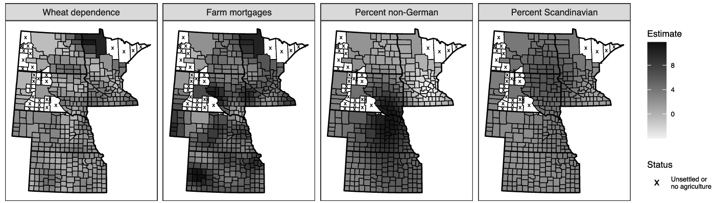
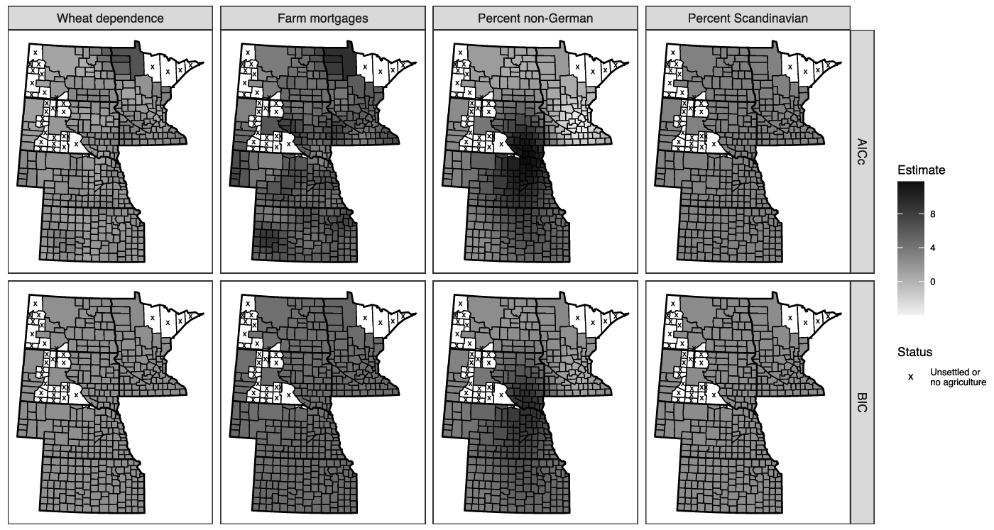
Whereas the global model indicates that the average vote share received by Populist candidates was strongly associated with the percentage of improved land devoted to wheat production, the distribution of local parameter estimates suggests that the effect was relatively weak in all but a handful of outlying locales.Footnote 4 Yet this is precisely where the global parameter estimate associated with wheat dependence happens to fall. The cases in question can be seen in figure 4, which projects the local point estimates from figure 3 on to the corresponding counties. Were it not for the small cluster of observations surrounding Marshall County, Minnesota, we would feel fairly confident claiming that wheat dependence exerted a weak effect on Populist voting throughout the region. Indeed, the value of the average local parameter estimate for wheat dependence is just 2.04, which is roughly one-fourth the size of the effect suggested by the global model. So while the relationship—or lack thereof—between wheat dependence and electoral Populism can plausibly be described in terms of a single number representing the typical effect, the global model leads us astray, turning an extreme and highly localized phenomenon into a seemingly general conclusion.
Local parameter estimates by variable.

The Varieties of Electoral Populism
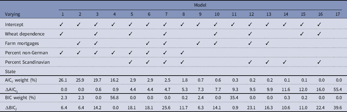
The degree of spatial variation in the association between average third-party vote share and a given covariate depends on how the spatially varying coefficient model is specified. To this point, we have assumed that the coefficients associated with each of the main predictors should be allowed to vary. Yet in much the same way that we can test for an interaction effect, we can use measures of model fit to systematically evaluate whether the inclusion of spatially varying coefficients is warranted for a given predictor or set of predictors, with the evaluation of the global model emerging as a special case. Rather than selecting a single model, I use measures of fit to construct a weighted composite of the local point estimates and standard errors produced by each model. For the purpose of this exercise, spatially invariant parameters are assumed to be constant across locales. I construct separate composites based on the AICc and BIC. The underlying weights are shown in table 1. Models are ranked according to their AICc weight, with the more conservative BIC weights serving as a check on the results.
Model definitions and weights by measure of fit

Note: Checkmarks denote which variables are allowed to vary in a given model.
As described above, model weights are a monotonic function of the underlying measures of fit and can thus be directly compared to assess differences in fit, though the relevant metric is the ratio of weights, as opposed to the difference. For ease of interpretation, I have included
 ${\rm{\Delta AI}}{{\rm{C}}_{{c_j}}}$
measures indicating the difference in fit between any given model j and the best-fitting model in the set according to the AICc. Using standard thresholds, a difference score of less than two indicates that a model is roughly on par with the best-fitting model and thus warrants serious consideration. Such is the case with the top four models in the set, which together account for roughly 88 percent of the weight going into the model-averaged estimates discussed below. Looking at the fit of these specifications, we find substantial evidence for the idea that, at minimum, the intercept and the percent non-German coefficient should be allowed to vary across counties, with the possibility of a more complex specification based on the inclusion of spatially varying wheat and/or mortgage coefficients. While a case can be made that we should consider any model with a difference score of less than 10, we still find no support for the global model, which is dramatically outpaced by every other model in the set, regardless of how we evaluate fit.
As expected, the BIC weights tend to concentrate on simpler models, though even here the majority of the weight is assigned to models that allow for variation in both intercept, as well as the association between Populist voting and the size of the non-German population. The difference in the distribution of weights based on the AICc and BIC are evident in the difference in the degree of variation in the model-averaged point estimates shown in figure 5. It is worth noting, however, that while the AICc-based estimates of the local wheat and mortgage coefficients vary considerably more than their BIC-based counterparts, they are still more conservative than the original estimates show in figure 4.Footnote 5 The latter figure is based on a single model in which all of the coefficients are allowed to vary from one county to the next. Rather than taking this particular model as given, the model-averaged estimates incorporate information from more conservative models as well (i.e., models in which one or coefficients is treated as fixed). To the extent that these simpler models are supported by the data, the set of local parameter estimates associated with any given variable is pulled toward these fixed values, thus productively stabilizing the results.
Local model-averaged parameter estimates by variable.

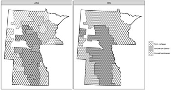
The fact that one or more coefficients varied across the sample is consistent with the idea that there were distinct varieties of electoral Populism in the American West. One way of thinking about this is to ask which covariates mattered where, allowing us to situate our claims in concrete geographies. Toward this end, we can use the model-averaged estimates to identify local regimes—regions of contiguous observations that share a common set of significant predictors (i.e., predictors with a model-averaged p-value of less than 0.10).Footnote 6 In this case, all the significant local effects are positive, allowing us to focus exclusively on the presence or absence of a significant effect. The results are shown in figure 6, which depicts the location of significant local coefficients for the following covariates: farm mortgages, percent non-German, and percent Scandinavian. Wheat dependence is omitted from the figure due to an absence of significant local effects. The symbols used to depict significant results can be overlaid on top of one other, producing a composite image representing the configuration of variables that are significant in any given locale. While this approach obscures the magnitude of the coefficients, it provides a clear, if simple, depiction of how the individual parameter surfaces intersected to create different varieties of electoral Populism. Information on the value of the underlying parameters can be readily gleaned from figure 5.
Local regime structures by measure of fit.

Two general trends stand out when looking at the spatial configuration of the resulting regime structures. First, in contrast to what we would expect given the prominence of the wheat-belt hypothesis in the existing literature, we find little support for the argument that third-party candidates fared better in wheat-dependent counties. While this association appeared quite sizable when looking at the global model from which we began, the introduction of spatially varying coefficients revealed that the observed relationship was limited to a handful counties in northwestern Minnesota. Yet once we account for the uncertainty in the underlying point estimates and the choice of model, the results are too noisy to warrant the claim that these counties constituted their own regime. Second, we find consistent support for the idea that there were geographically distinct varieties of ethnocultural Populism. When it came to the size of the Scandinavian population, the positive relationship between ethnic composition and average third-party vote share was relatively stable. This is apparent in the distribution of significant coefficients, as well as in the distribution of the underlying point estimates described at length above. The size of the ethnic German population, on the other hand, was not only negatively associated with the prevalence of third-party voting but also the distribution of significant estimates was limited to a north-south band running through central South Dakota, Kansas, and Nebraska. To be clear, economic factors were by no means irrelevant. There is clear evidence of a positive relationship between the prevalence of farm mortgages and the level of third-party support. Whether this relationship appears to be local or global depends on whether we use AICc or BIC to identify the regimes.
Conclusion
Historical analysis is defined not only by the use of historical materials but also by attention to the effects of the temporal and spatial context in which those materials were generated. Among quantitative researchers, this idea has come to be reflected in the use of models allowing for contextual effects through the introduction of parameter heterogeneity (e.g., Isaac and Griffin Reference Isaac and Griffin1989; Wawro and Katznelson Reference Wawro and Katznelson2014; Western and Kleykamp Reference Western and Kleykamp2004). Whereas existing research has tended to focus on variation in the association between variables over time, I have demonstrated how random effects eigenvector spatial filtering can be used to capture spatial heterogeneity in electoral data, producing a situated account of political behavior focusing on the distribution of local effects across concrete observations. Revisiting a critical case in the field of quantitative history, I show that the rise of electoral Populism in the American West was a spatially heterogeneous process characterized by marked variation in the correlates of third-party support. It is tempting to dismiss local variation as noise in an otherwise homogeneous process. Looking at the results, however, it is not just that point estimates differed a little bit from one place to the next, it is that the conventional global model is almost wholly incommensurate with the data at hand.
Of the various covariates considered, the size of the Scandinavian population was the only predictor whose effects could be reasonably and unambiguously approximated using a global model. This was not true for the other covariates. The results suggest that we should relax the homogeneity assumption for both the intercept, as well as the coefficient associated with the size of the German population, though there is support for more complex specifications as well. Once we begin making these changes, our findings regarding the size of the German population and the amount of improved land devoted to wheat production change in noticeable ways compared to what we would report if we relied solely on the global model.Footnote 7 In both cases, uncritical reliance on the global model causes us to mistake the mathematically particular for the historically general. The problem is especially pronounced in the case of wheat dependence, where we risk mistaking a local effect for a global one, as well as mistaking an effect that may not hold anywhere for an effect that holds everywhere!
These findings speak not only to longstanding debates over the nature of agrarian radicalism in the United States but also to the study of political action and the practice of quantitative research more generally. Insofar as it assumes a singular mapping between social and political cleavages, the problem with the standard global model is that it implicitly encodes the universalizing rhetoric of politicking into the resulting parameter estimates. In attempting to garner support for their cause, political leaders often appeal to simplified representations of the social world in which they draw sharp distinctions between “us” and “them” in an effort to bring these identities to life (see Bourdieu Reference Bourdieu1991: 180–93). Yet as noted by Gould, “people do not freely assemble their collective identities through ideational bricolage; instead, they are powerfully influenced by the patterns of social relationships in which they are implicated, in the sense that these patterns govern the plausibility of various identifications” (Reference Gould, Hanagan, Moch and te Brake1998: 51). This does not preclude the possibility of a global relationship between groups and parties. The point is that rather than taking this relationship as given, researchers are better served by methods that allow them to evaluate the extent to which this assumption is supported by the data, with the global model emerging as a special case.
This line of argument is consonant with recent work on the quantification of field effects in political sociology. The use of field theory has a long history in the study of political attitudes and behavior, going back to the foundational studies of Berelson et al. (Reference Berelson, Lazarsfeld and McPhee1954) and Campbell et al. (Reference Campbell, Converse, Miller and Stokes1960). Whereas these early works described the concept of the field in purely psychological terms, contemporary sociological approaches treat the political field as a competitive arena that can be described in terms of the distribution of potential forces across physical and/or social space (see Martin Reference Martin2003). The forces in question can be represented as a set of spatially situated vectors. Insofar as the magnitude of a given vector represents the strength of the field at a particular location, the strength of the field can be measured in terms of the average magnitude across the set of underlying vectors. Whether this is a meaningful representation of the field as a whole depends on the extent to which vectors are aligned across locales (i.e., on the extent to which the field is organized). Using classical geographically weighted regression to examine patterns of electoral behavior, Martin et al. (Reference Martin, Slez and Borkenhagen2016) show that this seemingly abstract formulation can be productively operationalized in terms of spatial heterogeneity and autocorrelation, with local regression coefficients serving a vectors. The analysis presented here can be read in a similar light, with the important caveat that the use of random effects eigenvector spatial filtering solves many of the problems typically associated with classical geographically weighted regression, thus improving on existing approaches.
The importance of spatial heterogeneity to historical and social scientific research is by no means limited to field theoretic accounts. To the extent that it implies different processes in different places, spatial heterogeneity is analogous to nonreplicability—a well-known concern that is said to have reached crisis-level proportions in recent years (see Freese and Peterson Reference Freese and Peterson2017). The roots of the perceived crisis in the social sciences can be traced in part to the use of statistical methods designed for a world governed by constant effects. While the assumption of constant effects may apply in fields such as classical physics, it is unlikely to hold when looking at social processes that are not only noisy but also contingent—varying over time, space, and groups. In short, social scientists are faced with an ontological reality that runs head to head with an outmoded epistemological desire to produce simple, stylized facts (Gelman Reference Gelman2015; Wood Reference Wood2000). As researchers become more accustomed to the idea of parameter heterogeneity as a standard feature of modern social science, the use of spatially varying coefficient models provides a clear way forward when working with spatial data.
From this perspective, the use of spatially varying coefficient models is about far more than just protecting against the limitations of the traditional global model. Among historically oriented social scientists, there is a growing willingness to embrace causal complexity as a fundamental feature of social life, as well as to build better, historically grounded explanations by transforming case-specific patterns into typological generalizations (e.g., Ragin Reference Ragin1987, Reference Ragin2000). The potential for typological generalization is evident when looking at patterns of third-party voting in the American West during the late nineteenth century. While factors such as the size of the Scandinavian population and, to a lesser extent, the prevalence of farm mortgages emerged as stable predictors of Populist support, counties could be systematically arrayed in terms of the extent to which the size of the ethnic German population was associated with third-party voting. Attending to the problem of spatial heterogeneity reveals a world in which a distinct brand of ethnic politics emerged in some locales but not others.
Though this finding is substantively meaningful in its own right, it is worth noting that this general approach to spatial heterogeneity can be pushed further still in an effort to elucidate the mechanisms underlying the variation in the local coefficients. For example, treating local coefficients as outcomes suggests that the strength of the relationship between third-party vote share and the size of the ethnic German population was positively associated with the prevalence of farm mortgages, suggesting that this particular form of ethnic politics was most pronounced in areas marked by financial hardship. While a full analysis of this sort is beyond the scope of this article, the analytic utility of spatially varying coefficient models and random effects eigenvector spatial filtering is apparent. In addition to allowing for the possibility of contextual variation, these techniques directly capture the extent to which this variation is spatially organized, thus avoiding the limitations of the conventional global model, while raising new questions regarding the origins of geographic differentiation. Favoring truth over simplicity, our ability to answer these types of second-order questions depends on our ability to first let the data speak for themselves.
Acknowledgments
I would like to thank Chad Borkenhagen, Clayton Childress, Jon Kropko, John Levi Martin, Daisuke Murakami, Jeff Olick, Nick Wilson, and two anonymous reviewers for their considerable insights. This work would not have gotten done without the support of the Writing with Randos group.