1 Introduction
Liquid metal batteries (LMBs) have many important characteristics for efficient practical use in combination with renewable energy sources on a national energy grid scale in the future. The relatively high voltage efficiency at high current densities of this storage technology is due to liquid–liquid electrode–electrolyte interfaces that enable high speed charge transfer, high total current capability, low ohmic losses as well as rapid mass transport of reactants and products to and from the electrode–electrolyte interfaces by means of liquid-state diffusion (Bradwell et al. Reference Bradwell, Kim, Sirk and Sadoway2012; Kim et al. Reference Kim, Boysen, Newhouse, Spatocco, Chung, Burke, Bradwell, Jiang, Tomaszowska, Wang, Wei, Ortiz, Barriga, Poizeau and Sadoway2013).
The liquid state of the main components necessitates consideration of the fluid dynamics in LMBs. A number of recent publications are devoted to the problem, e.g. investigating the possibility of the Tayler instability (Weber et al. Reference Weber, Galindo, Stefani and Weier2014; Herreman et al. Reference Herreman, Nore, Cappanera and Guermond2015; Weber et al. Reference Weber, Galindo, Stefani, Priede and Weier2015), thermal convection (Shen & Zikanov Reference Shen and Zikanov2016), observation of vortical flow in a LMB model (Kelley & Sadoway Reference Kelley and Sadoway2014) and a simplified model of sloshing in a three layer system (Zikanov Reference Zikanov2015). The main motivation of these investigations is to prevent the possibility of direct contact between the molten metal anode and cathode that may occur due to electro-magnetically driven destabilising interface motion. On the other hand, the controlled mixing enhances mass transport, improving the cell performance and preventing the accumulation of intermetallic compounds at the electrode–electrolyte interface.
LMBs are thought to be easily scalable at the cell level due to their simple construction using the natural density stratification of the liquid layers. Large cells of several cubic metres total volume have a potential to operate at very high power value (Bojarevics & Tucs Reference Bojarevics and Tucs2017). High current densities coupled to the magnetic field (created by the currents in the cell, the supply bars and the neighbour cells) lead to significant electromagnetic forces. Such forces in stratified liquid layers with large surface areas may cause a long wave interfacial instability as is well known in the case of Hall–Heroult cells (HHC), as first described by Sele (Reference Sele1977). The manifestation of this instability in LMBs is the subject of this paper.
In a typical HHC the electric current, of total magnitude 150–800 kA, enters the cell from the carbon anodes, passes through the liquid electrolyte and aluminium layer and exits via the carbon cathode blocks at the bottom of the cell. The liquid layers are relatively shallow, 4–30 cm in depth versus 4–20 m in horizontal dimension. The small relative depth of the layers and the small difference of the liquid densities facilitates the instability development.
The ratio of electrical conductivities of the cell materials is another significant parameter. The liquid metal is a better conductor (
 ${\sim}10^{6}~\text{S}~\text{m}^{-1}$
) than the carbon (
 ${\sim}10^{4}~\text{S}~\text{m}^{-1}$
), while the electrolyte is approximately two orders of magnitude less conductive (
 ${\sim}10^{2}~\text{S}~\text{m}^{-1}$
). The significantly lower conductivity of the electrolyte means that this layer is responsible for the majority of electrical losses in the cell. Joule heating is necessary to heat the cell and to keep the metal liquid, however the total voltage drop must be as low as possible in order to achieve a better electrical efficiency. A small perturbation of the interface between liquid layers may cause a substantial redistribution of the current in the cell.
First attempts to explain the interfacial instabilities were made by Sele (Reference Sele1977), Sneyd (Reference Sneyd1985), Urata (Reference Urata2016) and Moreau & Ziegler (Reference Moreau and Ziegler2016). A more involved understanding of the physical mechanism was provided by Bojarevics & Romerio (Reference Bojarevics and Romerio1994), Sneyd & Wang (Reference Sneyd and Wang1994), Bojarevics (Reference Bojarevics1998) and Davidson & Lindsay (Reference Davidson and Lindsay1998). The mechanism is based on the standing gravity wave modification due to the electric current redistribution. The electric current density in the electrolyte increases above the wave crests, resulting in a high density horizontal current in the shallow liquid metal layer. In the presence of a vertical magnetic field the electromagnetic force excites another standing wave mode orthogonal to the initial perturbation. The new wave mode is coupled to the original mode, and the oscillation frequency is shifted. The frequency shift increases with the rise of the magnetic field until at a critical value, when the two wave frequencies coincide, at which an exponential growth of the amplitude indicates the onset of instability. In general, the above process is described by the following set of equations:
 $$\begin{eqnarray}\displaystyle \unicode[STIX]{x2202}_{tt}\widehat{\unicode[STIX]{x1D701}}_{\boldsymbol{k}}+\unicode[STIX]{x1D714}_{\boldsymbol{k}}^{2}\widehat{\unicode[STIX]{x1D701}}_{\boldsymbol{k}}=E\mathop{\sum }_{\boldsymbol{k}^{\prime }\geqslant 0}\unicode[STIX]{x1D642}_{\boldsymbol{k}\boldsymbol{k}^{\prime }}\widehat{\unicode[STIX]{x1D701}}_{\boldsymbol{k}^{\prime }}, & & \displaystyle\end{eqnarray}$$
where
 $\widehat{\unicode[STIX]{x1D701}}_{\boldsymbol{k}}$
is a vector which represents the amplitudes of the original gravitational modes
 $\boldsymbol{k}=(k_{x},k_{y})$
,
 $\unicode[STIX]{x1D714}_{\boldsymbol{k}}^{2}$
is the matrix of the gravitational frequencies,
 $\unicode[STIX]{x1D642}_{\boldsymbol{k}\boldsymbol{k}^{\prime }}$
is the interaction matrix,
 $E$
is the dimensionless parameter characterising the electromagnetic forces. The mode coupling is included in
 $\unicode[STIX]{x1D642}_{\boldsymbol{k}\boldsymbol{k}^{\prime }}$
, where each column represents the Lorentz force (Fourier decomposed) in response to the gravitational wave modes. These coupled equations represent an eigenvalue problem for the square of the new complex frequencies
 $\unicode[STIX]{x1D707}$
(
 $\widehat{\unicode[STIX]{x1D701}}_{\boldsymbol{k}}\sim \text{e}^{\unicode[STIX]{x1D707}t}$
). The matrix
 $\unicode[STIX]{x1D642}_{\boldsymbol{k}\boldsymbol{k}^{\prime }}$
is real anti-symmetric, and in a general case the eigenvalues are shifted increasing the magnetic field (Bojarevics & Romerio Reference Bojarevics and Romerio1994). Onset of the instability starts at a critical value of
 $E$
at which the exponentially growing part of the complex eigenvalue
 $\unicode[STIX]{x1D707}$
appears. See also the paper by Antille & von Kaenel (Reference Antille and von Kaenel2002) where the numerical eigenvalue solution is analysed when approaching the instability threshold. A key point noted in the papers, is that the dominant contribution to the perturbed Lorentz force arises from the interaction between a horizontal current in the aluminium layer and the vertical component of the background magnetic field.
Davidson & Lindsay (Reference Davidson and Lindsay1998) derived a simple mechanical analogue which captures the basic features of the instability. The liquid aluminium layer is represented by a compound pendulum that consists of a large flat aluminium plate attached to a top surface by a light, rigid strut. The strut is pivoted at its top end so that the plate is free to swing along two horizontal axes
 $x$
and
 $y$
. The fluid system of infinite motion freedom is reduced to only two degrees of freedom. Zikanov (Reference Zikanov2015) constructed a similar mechanical model for instability description in the LMB taking into account an additional top liquid metal layer. The metal layers of the battery are represented by solid metal slabs rigidly attached to weightless rigid struts pivoted at the top. The free oscillations of the slabs imitate the sloshing motion of the liquid layers. The slabs are separated from each other by a layer of a poorly conducting electrolyte. Two destabilisation mechanisms were considered: (i) interaction of a purely vertical magnetic field and horizontal currents, similar to HHC, (ii) interaction between the current perturbations and the azimuthal self-magnetic field from the total vertical current. The first mechanism will occur in real batteries if a sufficiently strong vertical magnetic field is present due to the presence of an external current supply. The batteries of a square or a circular horizontal cross-section will be always unstable if even a small field is present. The second mechanism appears to be more challenging since the azimuthal magnetic field, unlike the vertical magnetic field, cannot be reduced via optimisation of the current supply lines unless they cross the liquid layer (Weber et al.
Reference Weber, Galindo, Stefani and Weier2014). The existence of the second instability type was predicted by Munger & Vincent (Reference Munger and Vincent2008) for the HHC case, yet needs more clarification for the LMB case. The approach developed by Davidson & Lindsay (Reference Davidson and Lindsay1998) and Zikanov (Reference Zikanov2015) is purely mechanical. However, the principal physical mechanism could be valid, due to the fact that sloshing motions generated in the shallow liquid layers are inherently large scale, and so their qualitative behaviour can be approximately described using the coupled pair of long wave modes approach.
More realistic fluid dynamic description can be achieved starting from the full set of Navier–Stokes equations by means of the shallow layer approximation and a systematic derivation of a set of coupled wave equations governing the three fluid layers. The hydrodynamic coupling is realised by pressure continuity at the common interfaces. The continuity of the electric potential and the supplied electric current will introduce the electromagnetic coupling of waves. In the following sections the linear stability of coupled modes will be investigated in the presence of a purely vertical magnetic field, accounting for the continuous electric current in the LMB model. The role of dissipation rate will be analysed using both analytical tools and numerical solutions. Analytical criteria for the cell stability will be established using approximations suitable for a practical cell design, including the solid bottom and top friction effects on the shallow layers.
2 Interfacial dynamics
Three layer liquid metal model under consideration.
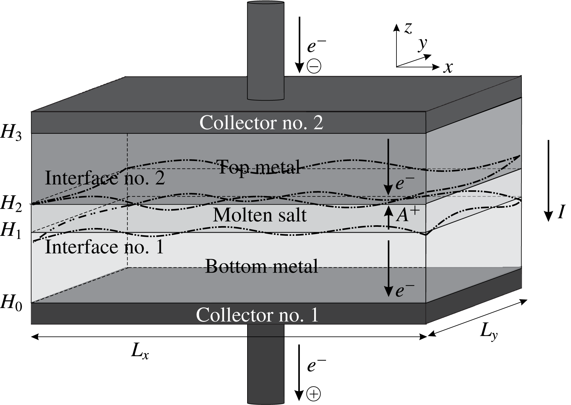
Hydrodynamics of the three density-stratified electrically conductive liquid layer system, schematically represented in figure 1, in the presence of electro-magnetic fields, is described by the following equations
 $$\begin{eqnarray}\displaystyle & \displaystyle \unicode[STIX]{x1D70C}\unicode[STIX]{x2202}_{t}u_{i}+\unicode[STIX]{x1D70C}u_{j}\unicode[STIX]{x2202}_{j}u_{i}=-\unicode[STIX]{x2202}_{i}(p+\unicode[STIX]{x1D70C}gz)+\unicode[STIX]{x2202}_{j}\unicode[STIX]{x1D70C}\unicode[STIX]{x1D708}(\unicode[STIX]{x2202}_{j}u_{i}+\unicode[STIX]{x2202}_{i}u_{j})+f_{i}, & \displaystyle\end{eqnarray}$$
 $$\begin{eqnarray}\displaystyle & \displaystyle \unicode[STIX]{x2202}_{i}u_{i}=0, & \displaystyle\end{eqnarray}$$
where the indices
 $i,j=1,2,3$
correspond to the coordinates
 $(x,y,z)$
, the velocity components are given as
 $(u_{1},u_{2},u_{3})$
, the summation over repeated indices is implied,
 $\unicode[STIX]{x1D70C}$
represents density,
 $\unicode[STIX]{x1D708}$
– effective viscosity,
 $g$
– the gravitational acceleration,
 $p$
– pressure and the vector of Lorentz force
 $\boldsymbol{f}=\boldsymbol{j}\times \boldsymbol{B}$
is computed in each of the 3 layers,
 $\boldsymbol{j}$
is the current density and
 $\boldsymbol{B}$
the magnetic field. In this paper the horizontal dimensions of the cell are assumed to be much larger than the vertical depth, so that the description can be based on a systematically derived shallow layer approximation. The velocity components in each layer can be represented as an expansion in a small aspect ratio parameter
 $\unicode[STIX]{x1D6FF}=\max h/\min L$
, where
 $h$
is a typical depth, for instance the unperturbed metal layer, and
 $L$
is the characteristic horizontal dimension (width of the cell):
 $$\begin{eqnarray}\displaystyle & \displaystyle u_{i}=u_{0i}(x,y,t)+\unicode[STIX]{x1D6FF}u_{1i}(x,y,\overline{z},t)+O(\unicode[STIX]{x1D6FF}^{2}),\quad i=1,2, & \displaystyle\end{eqnarray}$$
 $$\begin{eqnarray}\displaystyle & \displaystyle u_{3}=\unicode[STIX]{x1D6FF}u_{13}(x,y,\overline{z},t)+O(\unicode[STIX]{x1D6FF}^{2}), & \displaystyle\end{eqnarray}$$
where a stretched vertical coordinate
 $\overline{z}=z/\unicode[STIX]{x1D6FF}$
is introduced. The
 $u_{3}$
expansion starts with the
 $\unicode[STIX]{x1D6FF}$
order due to (2.2). If all three components of the electromagnetic force density are of the same order of magnitude:
 $f_{x}\sim f_{y}\sim f_{z}$
, and the horizontal pressure gradient components are of the same order as the corresponding force components:
 $\unicode[STIX]{x2202}_{i}p\approx f_{i}$
, then the vertical component of the gradient
 $\unicode[STIX]{x2202}_{3}p\sim -\unicode[STIX]{x1D70C}g\gg f_{z}$
. According to these estimates, the leading horizontal
 $(i=1,2)$
components of (2.1) are
 $$\begin{eqnarray}\displaystyle \unicode[STIX]{x1D70C}\unicode[STIX]{x2202}_{t}u_{0i}+\unicode[STIX]{x1D70C}u_{0j}\unicode[STIX]{x2202}_{j}u_{0i}=-\unicode[STIX]{x2202}_{i}p+\unicode[STIX]{x1D6FF}^{-1}\unicode[STIX]{x2202}_{\overline{z}}\unicode[STIX]{x1D70C}\unicode[STIX]{x1D708}\unicode[STIX]{x2202}_{\overline{z}}(u_{0i}+\unicode[STIX]{x1D6FF}u_{1i})+f_{i}. & & \displaystyle\end{eqnarray}$$
The vertical component of (2.1) gives the leading-order terms as:
 $$\begin{eqnarray}\displaystyle -\unicode[STIX]{x1D6FF}^{-1}\unicode[STIX]{x2202}_{\overline{z}}(p+\unicode[STIX]{x1D70C}g\unicode[STIX]{x1D6FF}\overline{z})+f_{z}=0. & & \displaystyle\end{eqnarray}$$
The hydrostatic pressure in the liquid layers adjacent to the interface
 $H_{1}(x,y,t)$
, see figure 1, can be expressed by
 $$\begin{eqnarray}\displaystyle p_{k_{1}}^{(1)}(x,y,z,t)=p_{p}^{(1)}(x,y,t)-\unicode[STIX]{x1D70C}_{k_{1}}g(z-H_{1})+\unicode[STIX]{x1D6FF}\int _{H_{1}(x,y,t)}^{z}f_{zk_{1}}\,\text{d}z, & & \displaystyle\end{eqnarray}$$
where the index
 $k_{1}=1,2$
stands for the layer number and
 $p_{p}^{(1)}$
is the reference pressure at the moving interface
 $z=H_{1}(x,y,t)$
. Similarly the same pressure can be referenced to the interface
 $H_{2}(x,y,t)$
, the corresponding pressure given by
 $$\begin{eqnarray}\displaystyle p_{k_{2}}^{(2)}(x,y,z,t)=p_{p}^{(2)}(x,y,t)-\unicode[STIX]{x1D70C}_{k_{2}}g(z-H_{2})+\unicode[STIX]{x1D6FF}\int _{H_{2}(x,y,t)}^{z}f_{zk_{2}}\,\text{d}z, & & \displaystyle\end{eqnarray}$$
where in this particular case
 $k_{2}=2,3$
. The respective horizontal gradients of the pressure required in the horizontal momentum equation (2.5) are:
 $$\begin{eqnarray}\displaystyle & \displaystyle \unicode[STIX]{x2202}_{i}p_{k_{1}}^{(1)}=\unicode[STIX]{x2202}_{i}p_{p}^{(1)}+\unicode[STIX]{x1D70C}_{k_{1}}g\unicode[STIX]{x2202}_{i}H_{1}+\unicode[STIX]{x1D6FF}\left[\int _{H_{1}}^{z}\unicode[STIX]{x2202}_{i}f_{z}\,\text{d}z-f_{z}(H_{1})\unicode[STIX]{x2202}_{i}H_{1}\right], & \displaystyle\end{eqnarray}$$
 $$\begin{eqnarray}\displaystyle & \displaystyle \unicode[STIX]{x2202}_{i}p_{k_{2}}^{(2)}=\unicode[STIX]{x2202}_{i}p_{p}^{(2)}+\unicode[STIX]{x1D70C}_{k_{2}}g\unicode[STIX]{x2202}_{i}H_{2}+\unicode[STIX]{x1D6FF}\left[\int _{H_{2}}^{z}\unicode[STIX]{x2202}_{i}f_{z}\,\text{d}z-f_{z}(H_{2})\unicode[STIX]{x2202}_{i}H_{2}\right]. & \displaystyle\end{eqnarray}$$
The next step is to introduce the depth averaging within each layer. The depth averaging for horizontal velocity components is performed in the following way:
 $$\begin{eqnarray}\displaystyle U_{ik}=h_{k}^{-1}\int _{H_{k-1}}^{H_{k}}u_{ik}(x,y,z)\,\text{d}z, & & \displaystyle\end{eqnarray}$$
where
 $k=1,2,3$
is the layer number (no summation over
 $k$
) and
 $h_{k}(x,y,t)=H_{k}-H_{k-1}$
is the local variable depth, see figure 1. The depth averaging can be applied to the continuity equation (2.2):
 $$\begin{eqnarray}\displaystyle h_{k}^{-1}\int _{H_{k-1}}^{H_{k}}(\unicode[STIX]{x2202}_{i}u_{i}+\unicode[STIX]{x2202}_{3}u_{3})\,\text{d}z & = & \displaystyle h_{k}^{-1}\left[\unicode[STIX]{x2202}_{i}\int _{H_{k-1}}^{H_{k}}u_{i}\,\text{d}z-u_{i}(H_{k})\unicode[STIX]{x2202}_{i}H_{k}+u_{i}(H_{k-1})\unicode[STIX]{x2202}_{i}H_{k-1}\right.\nonumber\\ \displaystyle & & \displaystyle \left.+\,u_{3}(H_{k})-u_{3}(H_{k-1})\right]=0,\end{eqnarray}$$
where
 $i=1,2$
. The vertical velocity
 $u_{3}$
at the
 $z=H_{k}(x,y,t)$
is given by the kinematic condition, stating that the interface moves with the local velocity:
 $$\begin{eqnarray}\displaystyle u_{3}(H_{k})=\unicode[STIX]{x2202}_{t}H_{k}+u_{i}(H_{k})\unicode[STIX]{x2202}_{i}H_{k}. & & \displaystyle\end{eqnarray}$$
Substituting (2.13) into (2.12) leads to
 $$\begin{eqnarray}\displaystyle \unicode[STIX]{x2202}_{t}h_{k}+\unicode[STIX]{x2202}_{i}(U_{ik}h_{k})=0. & & \displaystyle\end{eqnarray}$$
The last equation can be linearised if an additional approximation of a small wave amplitude is introduced:
 $h_{k}(x,y,t)=h_{0k}+\unicode[STIX]{x1D700}h_{k}^{\prime }(x,y,t)$
for the layer thickness or equivalently
 $H_{k}(x,y,t)=H_{0k}+\unicode[STIX]{x1D700}\unicode[STIX]{x1D701}_{k}(x,y,t)$
for the interface position, where the additional small parameter
 $\unicode[STIX]{x1D700}=\max A/h$
is introduced.
 $A$
is a typical wave amplitude and
 $h_{0k}$
,
 $H_{0k}$
are the unperturbed values,
 $\unicode[STIX]{x1D701}_{k}$
are the interfacial perturbations. For each particular layer the depth average horizontal velocity divergence can be expressed as:
 $$\begin{eqnarray}\displaystyle & \displaystyle \unicode[STIX]{x2202}_{i}U_{i1}=-\frac{\unicode[STIX]{x1D700}}{h_{01}}[\unicode[STIX]{x2202}_{t}\unicode[STIX]{x1D701}_{1}+\unicode[STIX]{x2202}_{i}(U_{i1}\unicode[STIX]{x1D701}_{1})], & \displaystyle\end{eqnarray}$$
 $$\begin{eqnarray}\displaystyle & \displaystyle \unicode[STIX]{x2202}_{i}U_{i2}=-\frac{\unicode[STIX]{x1D700}}{h_{02}}\{\unicode[STIX]{x2202}_{t}(\unicode[STIX]{x1D701}_{2}-\unicode[STIX]{x1D701}_{1})+\unicode[STIX]{x2202}_{i}[U_{i2}(\unicode[STIX]{x1D701}_{2}-\unicode[STIX]{x1D701}_{1})]\}, & \displaystyle\end{eqnarray}$$
 $$\begin{eqnarray}\displaystyle & \displaystyle \unicode[STIX]{x2202}_{i}U_{i3}=\frac{\unicode[STIX]{x1D700}}{h_{03}}[\unicode[STIX]{x2202}_{t}\unicode[STIX]{x1D701}_{2}+\unicode[STIX]{x2202}_{i}(U_{i3}\unicode[STIX]{x1D701}_{2})]. & \displaystyle\end{eqnarray}$$
The fixed top and bottom condition requires:
 $$\begin{eqnarray}\displaystyle h_{1}+h_{2}+h_{3}=H_{3}-H_{0}. & & \displaystyle\end{eqnarray}$$
In order to estimate the leading order of terms in the depth averaged momentum equations (2.5) dimensionless variables of order
 $O(1)$
are introduced using the following scaling:
 $L$
– for the coordinates
 $x,y$
;
 $h$
for a typical layer thickness;
 $\unicode[STIX]{x1D700}\sqrt{gh}$
– for the wave velocity;
 $L/\sqrt{gh}$
– for the time;
 $\unicode[STIX]{x1D70C}_{k}gh$
for the pressure (
 $k=1,2,3$
). For typical geometries considered in this paper
 $\unicode[STIX]{x1D6FF}=h/L\approx 0.2~\text{m}/8~\text{m}=0.0250\ll 1$
, whereas,
 $\unicode[STIX]{x1D700}=A/h\approx 0.005~\text{m}/0.2~\text{m}=0.0250\ll 1$
.
The horizontal pressure gradient from the expressions (2.9) and (2.10), neglecting terms of
 $\unicode[STIX]{x1D6FF}$
and higher order, can be substituted in the depth averaged, non-dimensionalised horizontal momentum equation (2.5). For the layers adjacent to the lower interface
 $H_{1}(x,y,t)$
the respective momentum equations are
 $$\begin{eqnarray}\displaystyle & \displaystyle \unicode[STIX]{x2202}_{t}U_{i1}+\unicode[STIX]{x1D700}U_{j1}\unicode[STIX]{x2202}_{j}U_{i1}=-\unicode[STIX]{x1D700}^{-1}\unicode[STIX]{x1D70C}_{1}^{-1}\unicode[STIX]{x2202}_{i}p_{p}^{(1)}-g\unicode[STIX]{x2202}_{i}\unicode[STIX]{x1D701}_{1}-k_{f1}U_{i1}+E_{1}F_{i1}, & \displaystyle\end{eqnarray}$$
 $$\begin{eqnarray}\displaystyle & \displaystyle \unicode[STIX]{x2202}_{t}U_{i2}+\unicode[STIX]{x1D700}U_{j2}\unicode[STIX]{x2202}_{j}U_{i2}=-\unicode[STIX]{x1D700}^{-1}\unicode[STIX]{x1D70C}_{2}^{-1}\unicode[STIX]{x2202}_{i}p_{p}^{(1)}-g\unicode[STIX]{x2202}_{i}\unicode[STIX]{x1D701}_{1}-k_{f2}U_{i2}+E_{2}F_{i2}, & \displaystyle\end{eqnarray}$$
where the depth averaged force
 $F_{i}$
is defined similarly to (2.11). For the upper interface
 $H_{2}(x,y,t)$
the respective equations are:
 $$\begin{eqnarray}\displaystyle & \displaystyle \unicode[STIX]{x2202}_{t}U_{i2}+\unicode[STIX]{x1D700}U_{j2}\unicode[STIX]{x2202}_{j}U_{i2}=-\unicode[STIX]{x1D700}^{-1}\unicode[STIX]{x1D70C}_{2}^{-1}\unicode[STIX]{x2202}_{i}p_{p}^{(2)}-g\unicode[STIX]{x2202}_{i}\unicode[STIX]{x1D701}_{2}-k_{f2}U_{i2}+E_{2}F_{i2}, & \displaystyle\end{eqnarray}$$
 $$\begin{eqnarray}\displaystyle & \displaystyle \unicode[STIX]{x2202}_{t}U_{i3}+\unicode[STIX]{x1D700}U_{j3}\unicode[STIX]{x2202}_{j}U_{i3}=-\unicode[STIX]{x1D700}^{-1}\unicode[STIX]{x1D70C}_{3}^{-1}\unicode[STIX]{x2202}_{i}p_{p}^{(2)}-g\unicode[STIX]{x2202}_{i}\unicode[STIX]{x1D701}_{2}-k_{f3}U_{i3}+E_{3}F_{i3}. & \displaystyle\end{eqnarray}$$
The equations (2.20) and (2.21) formally give the connection between the reference pressures
 $p_{p}^{(1)}$
and
 $p_{p}^{(2)}$
defined on the two interfaces, being valid in the same fluid layer
 $k=2$
(electrolyte):
 $p_{p}^{(1)}=p_{p}^{(2)}+\unicode[STIX]{x1D70C}_{2}gh_{2}(x,y,t)$
. The alternative representations (2.20) and (2.21) are required for the following wave equation derivation.
After the integration over depth the dissipative terms in (2.5) are replaced by empirical expressions used for the shallow layer approximation (Moreau & Evans Reference Moreau and Evans1984; Rodi Reference Rodi1987) using a linear in velocity friction law with the coefficients
 $k_{fk}$
. The electromagnetic interaction parameter (the ratio of electromagnetic force to the gravity force perturbation) is introduced as
 $E_{k}=IB_{0}/(L^{2}\unicode[STIX]{x1D70C}_{k}g\unicode[STIX]{x1D700}\unicode[STIX]{x1D6FF})$
, where
 $I$
is the total electric current,
 $B_{0}$
is a typical magnitude of magnetic field. The corresponding magnitude of
 $E$
can be estimated, using typical values for
 $I=10^{5}$
A,
 $B_{0}=10^{-3}$
T,
 $L=8$
m (width of cell),
 $\unicode[STIX]{x1D70C}=1.6\times 10^{3}~\text{kg}~\text{m}^{-3}$
(liquid magnesium for the top metal),
 $g=9.8~\text{m}~\text{s}^{-2}$
,
 $\unicode[STIX]{x1D700}=\unicode[STIX]{x1D6FF}=0.025$
:
 $E=0.32=O(1)$
. The electromagnetic term is of the same order of magnitude as the leading terms, while the nonlinear wave motion terms are of lower order (
 ${\sim}\unicode[STIX]{x1D700}$
) and will be neglected later in the linear theory, but retained for a numerical solution.
The wave equations for the coupled interfaces can be derived following the procedure described in Bojarevics (Reference Bojarevics1992):
(i) take time derivative of the non-dimensional linearised equations (2.15), (2.16):
(2.23) $$\begin{eqnarray}\displaystyle & \displaystyle \unicode[STIX]{x2202}_{it}U_{i1}=-\frac{\unicode[STIX]{x1D700}}{h_{01}}\unicode[STIX]{x2202}_{tt}\unicode[STIX]{x1D701}_{1}, & \displaystyle\end{eqnarray}$$
(2.24)$$\begin{eqnarray}\displaystyle & \displaystyle \unicode[STIX]{x2202}_{it}U_{i2}=-\frac{\unicode[STIX]{x1D700}}{h_{02}}\unicode[STIX]{x2202}_{tt}(\unicode[STIX]{x1D701}_{2}-\unicode[STIX]{x1D701}_{1}); & \displaystyle\end{eqnarray}$$
(ii) substitute (2.23), (2.24) into the horizontal divergence of (2.19), (2.20);
(iii) take the difference of the resulting equations.


This procedure eliminates the common unknown pressure
 $p_{p}^{(1)}$
on the interface
 $\unicode[STIX]{x1D701}_{1}$
:
 $$\begin{eqnarray}\displaystyle \unicode[STIX]{x1D6FC}_{1}\unicode[STIX]{x2202}_{tt}\unicode[STIX]{x1D701}_{1}+k_{fe1}\unicode[STIX]{x2202}_{t}\unicode[STIX]{x1D701}_{1}-\frac{\unicode[STIX]{x1D70C}_{2}}{h_{02}}\unicode[STIX]{x2202}_{tt}\unicode[STIX]{x1D701}_{2}-\frac{\unicode[STIX]{x1D70C}_{2}k_{f2}}{h_{02}}\unicode[STIX]{x2202}_{t}\unicode[STIX]{x1D701}_{2} & = & \displaystyle R_{1}\unicode[STIX]{x2202}_{jj}\unicode[STIX]{x1D701}_{1}-\unicode[STIX]{x1D70C}_{1}E_{1}\unicode[STIX]{x2202}_{j}F_{i1}+\unicode[STIX]{x1D70C}_{2}E_{2}\unicode[STIX]{x2202}_{j}F_{i2}\nonumber\\ \displaystyle & & \displaystyle +\,\unicode[STIX]{x1D700}[\unicode[STIX]{x1D70C}_{1}\unicode[STIX]{x2202}_{j}(U_{i1}\unicode[STIX]{x2202}_{i}U_{j1})-\unicode[STIX]{x1D70C}_{2}\unicode[STIX]{x2202}_{j}(U_{i2}\unicode[STIX]{x2202}_{i}U_{j2})].\end{eqnarray}$$
The corresponding boundary conditions for the normal velocity
 $u_{n}=0$
at the side walls can be obtained by taking the difference between (2.19) and (2.20) to eliminate the common pressure at the interface
 $\unicode[STIX]{x1D701}_{1}$
:
 $$\begin{eqnarray}\displaystyle \unicode[STIX]{x2202}_{n}\unicode[STIX]{x1D701}_{1}=(\unicode[STIX]{x1D70C}_{1}E_{1}F_{n1}-\unicode[STIX]{x1D70C}_{2}E_{2}F_{n2})/R_{1}. & & \displaystyle\end{eqnarray}$$
In a similar manner the wave equation for the upper interface
 $\unicode[STIX]{x1D701}_{2}$
can be obtained:
 $$\begin{eqnarray}\displaystyle \unicode[STIX]{x1D6FC}_{2}\unicode[STIX]{x2202}_{tt}\unicode[STIX]{x1D701}_{2}+k_{fe2}\unicode[STIX]{x2202}_{t}\unicode[STIX]{x1D701}_{2}-\frac{\unicode[STIX]{x1D70C}_{2}}{h_{02}}\unicode[STIX]{x2202}_{tt}\unicode[STIX]{x1D701}_{1}-\frac{\unicode[STIX]{x1D70C}_{2}k_{f2}}{h_{02}}\unicode[STIX]{x2202}_{t}\unicode[STIX]{x1D701}_{1} & = & \displaystyle R_{2}\unicode[STIX]{x2202}_{jj}\unicode[STIX]{x1D701}_{2}-\unicode[STIX]{x1D70C}_{2}E_{2}\unicode[STIX]{x2202}_{j}F_{i2}+\unicode[STIX]{x1D70C}_{3}E_{3}\unicode[STIX]{x2202}_{j}F_{i3}\nonumber\\ \displaystyle & & \displaystyle +\,\unicode[STIX]{x1D700}[\unicode[STIX]{x1D70C}_{2}\unicode[STIX]{x2202}_{j}(U_{i2}\unicode[STIX]{x2202}_{i}U_{j2})-\unicode[STIX]{x1D70C}_{3}\unicode[STIX]{x2202}_{j}(U_{i3}\unicode[STIX]{x2202}_{i}U_{j3})],\end{eqnarray}$$
and the corresponding boundary conditions are
 $$\begin{eqnarray}\displaystyle \unicode[STIX]{x2202}_{n}\unicode[STIX]{x1D701}_{2}=(\unicode[STIX]{x1D70C}_{2}E_{2}F_{n2}-\unicode[STIX]{x1D70C}_{3}E_{3}F_{n3})/R_{2}. & & \displaystyle\end{eqnarray}$$
The new constants introduced in the above equations are defined as:
 $$\begin{eqnarray}\displaystyle \unicode[STIX]{x1D6FC}_{1}=\frac{\unicode[STIX]{x1D70C}_{1}}{h_{01}}+\frac{\unicode[STIX]{x1D70C}_{2}}{h_{02}},\quad \unicode[STIX]{x1D6FC}_{2}=\frac{\unicode[STIX]{x1D70C}_{2}}{h_{02}}+\frac{\unicode[STIX]{x1D70C}_{3}}{h_{03}}, & & \displaystyle\end{eqnarray}$$
 $$\begin{eqnarray}\displaystyle k_{fe1}=\frac{\unicode[STIX]{x1D70C}_{1}k_{f1}}{h_{01}}+\frac{\unicode[STIX]{x1D70C}_{2}k_{f2}}{h_{02}},\quad k_{fe2}=\frac{\unicode[STIX]{x1D70C}_{3}k_{f3}}{h_{03}}+\frac{\unicode[STIX]{x1D70C}_{2}k_{f2}}{h_{02}}, & & \displaystyle\end{eqnarray}$$
 $$\begin{eqnarray}\displaystyle R_{1}=(\unicode[STIX]{x1D70C}_{1}-\unicode[STIX]{x1D70C}_{2})g,\quad R_{2}=(\unicode[STIX]{x1D70C}_{2}-\unicode[STIX]{x1D70C}_{3})g. & & \displaystyle\end{eqnarray}$$
Note, that in (2.25) and (2.27) summation over repeated indices is limited to the two horizontal dimensions. As can be seen from (2.25) and (2.27), both interfaces cannot be considered independently due to the presence of coupling terms. In the following we will assume that the interfacial friction
 $k_{f2}$
is negligible. The set of the equations in the electrically non-conductive limit and in the absence of viscous dissipation is in correspondence with the set of the equations obtained by Robino, Brandt & Weigle (Reference Robino, Brandt and Weigle2001) derived for the dynamics of internal solitary waves in a stratified 3 layer ocean. The aluminium electrolysis cell magnetohydrodynamic (MHD) wave model can be recovered if
 $\unicode[STIX]{x1D701}_{2}=0$
in (2.25).
3 Electric current flow
For energy storage and supply the LMBs must operate in two regimes: charge and discharge, resulting in the current flowing upwards or downwards. In this paper only the charging process is considered due to the physical symmetry of both operational regimes. The current flow in the layered structure is illustrated in figure 1. Similarly to Davidson & Lindsay (Reference Davidson and Lindsay1998), we assume that the characteristic time scale for the wave motion is much larger than the diffusion time of the magnetic field to satisfy the low magnetic Reynolds number approximation, leading to
 $Rm=\unicode[STIX]{x1D707}\unicode[STIX]{x1D70E}Uh\ll 1$
, where
 $\unicode[STIX]{x1D707}$
is the magnetic permeability,
 $\unicode[STIX]{x1D70E}$
the electrical conductivity,
 $U$
is a typical velocity. Using typical values for the liquid metal
 $\unicode[STIX]{x1D707}=4\unicode[STIX]{x03C0}\times 10^{-7}~\text{H}~\text{m}^{-1}$
,
 $\unicode[STIX]{x1D70E}=3.65\times 10^{6}~\text{S}~\text{m}^{-1}$
,
 $U=0.01~\text{m}~\text{s}^{-1}$
,
 $h=0.1$
m the estimated value of
 $Rm\approx 0.004$
. A similar estimate can be obtained for the ratio of the electric current magnetically induced by the wave motion relative to the basic imposed current density:
 $\unicode[STIX]{x1D70E}\unicode[STIX]{x1D700}\sqrt{gh}B_{0}/(I/L^{2})\approx 0.001$
.
In the low
 $Rm$
approximation and when the flow effect on the current distribution is neglected, the electric current can be expressed as
 $$\begin{eqnarray}\displaystyle \boldsymbol{j}_{k}=-\unicode[STIX]{x1D70E}_{k}\unicode[STIX]{x1D735}\unicode[STIX]{x1D711}_{k} & & \displaystyle\end{eqnarray}$$
and is described by a set of coupled Laplace equations for the electric potential
 $\unicode[STIX]{x1D711}_{k}(x,y,z)$
:
 $$\begin{eqnarray}\displaystyle \unicode[STIX]{x2202}_{ii}\unicode[STIX]{x1D711}_{k}=0, & & \displaystyle\end{eqnarray}$$
where
 $k=1,2,3$
corresponds to the layer number. The continuity conditions for the electric potential and the normal current component
 $\boldsymbol{j}\boldsymbol{\cdot }\boldsymbol{n}$
at the interfaces
 $z=H_{m}$
 $(m=1,2)$
are
 $$\begin{eqnarray}\displaystyle & \displaystyle \unicode[STIX]{x1D711}_{m}=\unicode[STIX]{x1D711}_{m+1}, & \displaystyle\end{eqnarray}$$
 $$\begin{eqnarray}\displaystyle & \displaystyle \unicode[STIX]{x1D70E}_{m+1}\unicode[STIX]{x2202}_{n}\unicode[STIX]{x1D711}_{m+1}=\unicode[STIX]{x1D70E}_{m}\unicode[STIX]{x2202}_{n}\unicode[STIX]{x1D711}_{m}. & \displaystyle\end{eqnarray}$$
The normal derivatives at the deformed interfaces are defined as (assuming the summation over the repeated index
 $i$
only):
 $$\begin{eqnarray}\displaystyle \unicode[STIX]{x2202}_{n}\unicode[STIX]{x1D711}_{k}=\frac{\unicode[STIX]{x2202}_{z}\unicode[STIX]{x1D711}_{k}-\unicode[STIX]{x2202}_{i}H_{k}\unicode[STIX]{x2202}_{i}\unicode[STIX]{x1D711}_{k}}{(1+\unicode[STIX]{x2202}_{i}H_{k}\unicode[STIX]{x2202}_{i}H_{k})^{1/2}}. & & \displaystyle\end{eqnarray}$$
With (3.5) the current continuity (3.4) at the interfaces
 $H_{1}$
and
 $H_{2}$
can be written explicitly in the non-dimensional form in order to estimate the leading-order terms:
 $$\begin{eqnarray}\displaystyle & \displaystyle s_{1}\unicode[STIX]{x1D6FF}^{2}(\unicode[STIX]{x2202}_{\overline{z}}\unicode[STIX]{x1D711}_{2}-\unicode[STIX]{x1D700}\unicode[STIX]{x1D6FF}^{2}\unicode[STIX]{x2202}_{i}\overline{\unicode[STIX]{x1D701}}_{1}\unicode[STIX]{x2202}_{i}\unicode[STIX]{x1D711}_{2})=\unicode[STIX]{x2202}_{\overline{z}}\unicode[STIX]{x1D711}_{1}-\unicode[STIX]{x1D700}\unicode[STIX]{x1D6FF}^{2}\unicode[STIX]{x2202}_{i}\overline{\unicode[STIX]{x1D701}}_{1}\unicode[STIX]{x2202}_{i}\unicode[STIX]{x1D711}_{1}, & \displaystyle\end{eqnarray}$$
 $$\begin{eqnarray}\displaystyle & \displaystyle \unicode[STIX]{x2202}_{\overline{z}}\unicode[STIX]{x1D711}_{3}-\unicode[STIX]{x1D700}\unicode[STIX]{x1D6FF}^{2}\unicode[STIX]{x2202}_{i}\overline{\unicode[STIX]{x1D701}}_{2}\unicode[STIX]{x2202}_{i}\unicode[STIX]{x1D711}_{3}=s_{3}\unicode[STIX]{x1D6FF}^{2}(\unicode[STIX]{x2202}_{\overline{z}}\unicode[STIX]{x1D711}_{2}-\unicode[STIX]{x1D700}\unicode[STIX]{x1D6FF}^{2}\unicode[STIX]{x2202}_{i}\overline{\unicode[STIX]{x1D701}}_{2}\unicode[STIX]{x2202}_{i}\unicode[STIX]{x1D711}_{2}), & \displaystyle\end{eqnarray}$$
where the four orders of magnitude difference in the electrical conductivities permit us to define
 $\unicode[STIX]{x1D70E}_{2}/\unicode[STIX]{x1D70E}_{1}=s_{1}\unicode[STIX]{x1D6FF}^{2}$
,
 $\unicode[STIX]{x1D70E}_{2}/\unicode[STIX]{x1D70E}_{3}=s_{3}\unicode[STIX]{x1D6FF}^{2}$
and the stretched
 $\overline{\unicode[STIX]{x1D701}}_{k}=\unicode[STIX]{x1D701}_{k}/\unicode[STIX]{x1D6FF}$
. These definitions allow us to compare numerically the electrical conductivities in the poorly conducting electrolyte relative to the well-conducting liquid metals, and the effect of the small depth (
 ${\sim}\unicode[STIX]{x1D6FF}$
) of the layers. The side walls of the domain are considered to be electrically insulating:
 $$\begin{eqnarray}\displaystyle (\unicode[STIX]{x2202}_{n}\unicode[STIX]{x1D711}_{k})_{x=0,L_{x};y=0,L_{y}}=0. & & \displaystyle\end{eqnarray}$$
In this paper, we assume that the applied current distributions at the top and the bottom are uniform, equal and the interfacial perturbation do not influence the electric current distributions in the collectors:
 $$\begin{eqnarray}\displaystyle (j)_{\overline{z}=\overline{H}_{0}}=(j)_{\overline{z}=\overline{H}_{3}}=-j, & & \displaystyle\end{eqnarray}$$
where
 $\overline{H}_{k}=H_{k}/\unicode[STIX]{x1D6FF}$
. In principle,
 $j(x,y,t)$
could be used, however requiring an external circuit solution.
The set of Laplace equations (3.2) can be rewritten in a non-dimensional form
 $$\begin{eqnarray}\displaystyle \unicode[STIX]{x1D6FF}^{2}\unicode[STIX]{x2202}_{ii}\unicode[STIX]{x1D711}_{k}+\unicode[STIX]{x2202}_{\overline{z}\overline{z}}\unicode[STIX]{x1D711}_{k}=0. & & \displaystyle\end{eqnarray}$$
The shallow layer approximation requires that the potential is expanded in terms of the parameter
 $\unicode[STIX]{x1D6FF}$
:
 $$\begin{eqnarray}\displaystyle \unicode[STIX]{x1D711}_{k}(x,y,\overline{z},t)=\unicode[STIX]{x1D711}_{0k}+\unicode[STIX]{x1D6FF}\unicode[STIX]{x1D711}_{1k}+\unicode[STIX]{x1D6FF}^{2}\unicode[STIX]{x1D711}_{2k}+O(\unicode[STIX]{x1D6FF}^{3}), & & \displaystyle\end{eqnarray}$$
where the expansion terms are expressed in a similar manner as in Bojarevics & Romerio (Reference Bojarevics and Romerio1994):
 $$\begin{eqnarray}\displaystyle & \displaystyle \unicode[STIX]{x1D711}_{0k}=(a_{k}+\unicode[STIX]{x1D700}A_{k})\overline{z}+(b_{k}+\unicode[STIX]{x1D700}B_{k}), & \displaystyle\end{eqnarray}$$
 $$\begin{eqnarray}\displaystyle & \displaystyle \unicode[STIX]{x1D711}_{1k}=(c_{k}+\unicode[STIX]{x1D700}C_{k})\overline{z}+(d_{k}+\unicode[STIX]{x1D700}D_{k}), & \displaystyle\end{eqnarray}$$
 $$\begin{eqnarray}\displaystyle & \displaystyle \unicode[STIX]{x1D711}_{2k}=(e_{k}+\unicode[STIX]{x1D700}E_{k})\overline{z}+(g_{k}+\unicode[STIX]{x1D700}G_{k})-{\textstyle \frac{1}{6}}\overline{z}^{3}\unicode[STIX]{x2202}_{ii}(a_{k}+\unicode[STIX]{x1D700}A_{k})-{\textstyle \frac{1}{2}}\overline{z}^{2}\unicode[STIX]{x2202}_{ii}(b_{k}+\unicode[STIX]{x1D700}B_{k}), & \displaystyle\end{eqnarray}$$
where
 $a$
,
 $b$
,
 $c$
,
 $d$
,
 $e$
,
 $g$
are the coordinate,
 $x$
and
 $y$
, dependent functions that correspond to the unperturbed interfaces. The functions
 $A$
,
 $B$
,
 $C$
,
 $D$
,
 $E$
,
 $G$
are
 $x$
,
 $y$
and time
 $t$
dependent, corresponding to the perturbed interfaces. Taking into account the previously described boundary conditions and neglecting the higher-order terms, the unknown coefficients can be determined as shown in the appendix A by equalising the similar order of magnitude terms. The resulting perturbed potential equations reflect the continuity of the electric potential and the electric current between the layers.
The final set of equations (A 17) and (A 18) governing the electric current distribution in the system is obtained by introducing the perturbed potentials in both metal layers:
 $\unicode[STIX]{x1D6F7}_{1}=\unicode[STIX]{x1D700}B_{1}$
,
 $\unicode[STIX]{x1D6F7}_{3}=\unicode[STIX]{x1D700}B_{3}$
. The dimensional electric potential perturbations are linearly related to the respective interface perturbations:
 $$\begin{eqnarray}\displaystyle & \displaystyle h_{01}h_{02}\unicode[STIX]{x2202}_{ii}\unicode[STIX]{x1D6F7}_{1}+\frac{\unicode[STIX]{x1D70E}_{2}}{\unicode[STIX]{x1D70E}_{1}}(\unicode[STIX]{x1D6F7}_{3}-\unicode[STIX]{x1D6F7}_{1})=\frac{j}{\unicode[STIX]{x1D70E}_{1}}(\unicode[STIX]{x1D701}_{2}-\unicode[STIX]{x1D701}_{1}), & \displaystyle\end{eqnarray}$$
 $$\begin{eqnarray}\displaystyle & \displaystyle h_{02}h_{03}\unicode[STIX]{x2202}_{ii}\unicode[STIX]{x1D6F7}_{3}-\frac{\unicode[STIX]{x1D70E}_{2}}{\unicode[STIX]{x1D70E}_{3}}(\unicode[STIX]{x1D6F7}_{3}-\unicode[STIX]{x1D6F7}_{1})=-\frac{j}{\unicode[STIX]{x1D70E}_{3}}(\unicode[STIX]{x1D701}_{2}-\unicode[STIX]{x1D701}_{1}), & \displaystyle\end{eqnarray}$$
where
 $h_{0k}$
are the unperturbed layer thicknesses. The perturbed potential equations can be rewritten in an equivalent form using the fact that the perturbed current is completely enclosed within the 3 liquid layer system, resulting in the relation (A 21) between the potentials
 $\unicode[STIX]{x1D6F7}_{1}$
and
 $\unicode[STIX]{x1D6F7}_{3}$
. This relation permits us to solve the formally decoupled equations:
 $$\begin{eqnarray}\displaystyle & \displaystyle h_{01}h_{02}\unicode[STIX]{x2202}_{ii}\unicode[STIX]{x1D6F7}_{1}-\unicode[STIX]{x1D70E}_{e,1}\unicode[STIX]{x1D6F7}_{1}=\frac{j}{\unicode[STIX]{x1D70E}_{1}}(\unicode[STIX]{x1D701}_{2}-\unicode[STIX]{x1D701}_{1}), & \displaystyle\end{eqnarray}$$
 $$\begin{eqnarray}\displaystyle & \displaystyle h_{02}h_{03}\unicode[STIX]{x2202}_{ii}\unicode[STIX]{x1D6F7}_{3}-\unicode[STIX]{x1D70E}_{e,2}\unicode[STIX]{x1D6F7}_{3}=-\frac{j}{\unicode[STIX]{x1D70E}_{3}}(\unicode[STIX]{x1D701}_{2}-\unicode[STIX]{x1D701}_{1}), & \displaystyle\end{eqnarray}$$
where the effective conductivities replace the potential difference in (3.15), (3.16):
 $$\begin{eqnarray}\displaystyle & \displaystyle \unicode[STIX]{x1D70E}_{e,1}=\frac{\unicode[STIX]{x1D70E}_{2}}{\unicode[STIX]{x1D70E}_{1}}\left(1+\frac{\unicode[STIX]{x1D70E}_{1}}{\unicode[STIX]{x1D70E}_{3}}\frac{h_{01}}{h_{03}}\right), & \displaystyle\end{eqnarray}$$
 $$\begin{eqnarray}\displaystyle & \displaystyle \unicode[STIX]{x1D70E}_{e,2}=\frac{\unicode[STIX]{x1D70E}_{2}}{\unicode[STIX]{x1D70E}_{3}}\left(1+\frac{\unicode[STIX]{x1D70E}_{3}}{\unicode[STIX]{x1D70E}_{1}}\frac{h_{03}}{h_{01}}\right). & \displaystyle\end{eqnarray}$$
The current distribution in the electrolyte is almost purely vertical due to fact that
 $\unicode[STIX]{x1D70E}_{2}\ll \unicode[STIX]{x1D70E}_{1}\sim \unicode[STIX]{x1D70E}_{3}$
(similarly to Zikanov (Reference Zikanov2018)). According to (3.15) and (3.16), the current flow is perturbed by the electrolyte thickness perturbations. Finally, the corresponding dimensional current components can be expressed as
 $$\begin{eqnarray}\displaystyle & \displaystyle \boldsymbol{j}_{1}=-\unicode[STIX]{x1D70E}_{1}\left(\unicode[STIX]{x2202}_{x}\unicode[STIX]{x1D6F7}_{1},\unicode[STIX]{x2202}_{y}\unicode[STIX]{x1D6F7}_{1},\frac{j}{\unicode[STIX]{x1D70E}_{1}}+(H_{0}-z)\unicode[STIX]{x2202}_{ii}\unicode[STIX]{x1D6F7}_{1}\right), & \displaystyle\end{eqnarray}$$
 $$\begin{eqnarray}\displaystyle & \displaystyle \boldsymbol{j}_{2}=-\unicode[STIX]{x1D70E}_{2}\left(0,0,\left(1-\frac{h_{2}-h_{02}}{h_{02}}\right)\frac{j}{\unicode[STIX]{x1D70E}_{2}}+\frac{\unicode[STIX]{x1D6F7}_{3}-\unicode[STIX]{x1D6F7}_{1}}{h_{02}}\right), & \displaystyle\end{eqnarray}$$
 $$\begin{eqnarray}\displaystyle & \displaystyle \boldsymbol{j}_{3}=-\unicode[STIX]{x1D70E}_{3}\left(\unicode[STIX]{x2202}_{x}\unicode[STIX]{x1D6F7}_{3},\unicode[STIX]{x2202}_{y}\unicode[STIX]{x1D6F7}_{3},\frac{j}{\unicode[STIX]{x1D70E}_{3}}+(H_{3}-z)\unicode[STIX]{x2202}_{ii}\unicode[STIX]{x1D6F7}_{3}\right). & \displaystyle\end{eqnarray}$$
In the following section it will be shown that some of these perturbations may become electromagnetically coupled due to the presence of a magnetic field and may lead to an instability resulting in a short circuit state in the extreme case.
4 Linear stability analysis
4.1 Coupled 3 layer problem
The wave equations (2.25)–(2.28) can be linearised neglecting the
 $\unicode[STIX]{x1D700}$
-order nonlinear terms and assuming a given magnetic field distribution, which can be expanded in terms of the small parameter
 $\unicode[STIX]{x1D6FF}$
:
 $\boldsymbol{B}(x,y,z)=\boldsymbol{B}^{0}(x,y)+\unicode[STIX]{x1D6FF}\boldsymbol{B}^{1}(x,y,z)+O(\unicode[STIX]{x1D6FF}^{2})$
. This expansion follows the same principle as the electric current representation
 $\boldsymbol{j}(x,y,z)=\boldsymbol{j}^{0}(x,y)+\unicode[STIX]{x1D6FF}\boldsymbol{j}^{1}(x,y,z)+O(\unicode[STIX]{x1D6FF}^{2})$
. At this stage we assume that the leading part of the magnetic field is caused by external sources (connectors, supply lines, neighbouring batteries etc.), therefore
 $\unicode[STIX]{x1D735}\times \boldsymbol{B}^{0}=0$
in the liquid zone. This allows us to neglect the electro-magnetic force components resulting from the horizontal magnetic field interaction with the vertical unperturbed current:
 $-j_{z}^{0}B_{y}^{0}\boldsymbol{e}_{x}$
,
 $j_{z}^{0}B_{x}^{0}\boldsymbol{e}_{y}$
due to the zero contribution to the horizontal divergence term in (2.25), (2.27):
 $j_{z}^{0}(\unicode[STIX]{x2202}_{y}B_{x}^{0}-\unicode[STIX]{x2202}_{x}B_{y}^{0})\boldsymbol{e}_{z}=0$
. The leading horizontal force components contain the horizontal electric current and the vertical magnetic field:
 $j_{y}^{1}B_{z}^{0}\boldsymbol{e}_{x}$
,
 $-j_{x}^{1}B_{z}^{0}\boldsymbol{e}_{y}$
, noting that
 $j_{z}^{1}$
is
 $\unicode[STIX]{x1D6FF}$
order lower than the horizontal perturbation current. This confirms the assumptions made in § 1 and implied in the previous studies on MHD stability of HHC that the magnetic field is purely vertical
 $\boldsymbol{B}=\boldsymbol{B}^{0}=B_{z}^{0}(x,y)\boldsymbol{e}_{z}$
and it is caused by external sources. Note also that the leading-order fluid flow is not affected by the curl of electro-magnetic force composed of the unperturbed vertical current and the zero-order horizontal magnetic field because
 $\unicode[STIX]{x1D735}\times \boldsymbol{f}^{0}=\unicode[STIX]{x1D735}\times (j_{z}^{0}\boldsymbol{e}_{z}\times \boldsymbol{B}^{0}(x,y))=-(j_{z}^{0}\boldsymbol{e}_{z}\boldsymbol{\cdot }\unicode[STIX]{x1D735})\boldsymbol{B}^{0}=\mathbf{0}$
, which is valid for thin liquid layers where the leading-order magnetic field is practically depth independent.
The set of the wave equations for this case has the following form, after assuming that the friction at the electrolyte top and bottom is negligible in comparison to the friction at the solid top and bottom:
 $$\begin{eqnarray}\displaystyle & \displaystyle \unicode[STIX]{x1D6FC}_{1}\unicode[STIX]{x2202}_{tt}\unicode[STIX]{x1D701}_{1}+k_{fe1}\unicode[STIX]{x2202}_{t}\unicode[STIX]{x1D701}_{1}-\frac{\unicode[STIX]{x1D70C}_{2}}{h_{2}}\unicode[STIX]{x2202}_{tt}\unicode[STIX]{x1D701}_{2}=R_{1}\unicode[STIX]{x2202}_{jj}\unicode[STIX]{x1D701}_{1}+\unicode[STIX]{x1D70E}_{1}(\unicode[STIX]{x2202}_{y}\unicode[STIX]{x1D6F7}_{1}\unicode[STIX]{x2202}_{x}B_{z}^{0}-\unicode[STIX]{x2202}_{x}\unicode[STIX]{x1D6F7}_{1}\unicode[STIX]{x2202}_{y}B_{z}^{0}), & \displaystyle\end{eqnarray}$$
 $$\begin{eqnarray}\displaystyle & \displaystyle \unicode[STIX]{x1D6FC}_{2}\unicode[STIX]{x2202}_{tt}\unicode[STIX]{x1D701}_{2}+k_{fe3}\unicode[STIX]{x2202}_{t}\unicode[STIX]{x1D701}_{2}-\frac{\unicode[STIX]{x1D70C}_{2}}{h_{2}}\unicode[STIX]{x2202}_{tt}\unicode[STIX]{x1D701}_{1}=R_{2}\unicode[STIX]{x2202}_{jj}\unicode[STIX]{x1D701}_{2}+\unicode[STIX]{x1D70E}_{3}(\unicode[STIX]{x2202}_{x}\unicode[STIX]{x1D6F7}_{3}\unicode[STIX]{x2202}_{y}B_{z}^{0}-\unicode[STIX]{x2202}_{y}\unicode[STIX]{x1D6F7}_{3}\unicode[STIX]{x2202}_{x}B_{z}^{0}), & \displaystyle\end{eqnarray}$$
with the boundary conditions at the side walls:
 $$\begin{eqnarray}\displaystyle & \displaystyle R_{1}\unicode[STIX]{x2202}_{n}\unicode[STIX]{x1D701}_{1}-B_{z}^{0}\unicode[STIX]{x1D70E}_{1}(n_{y}\unicode[STIX]{x2202}_{x}\unicode[STIX]{x1D6F7}_{1}-n_{x}\unicode[STIX]{x2202}_{y}\unicode[STIX]{x1D6F7}_{1})=0, & \displaystyle\end{eqnarray}$$
 $$\begin{eqnarray}\displaystyle & \displaystyle R_{2}\unicode[STIX]{x2202}_{n}\unicode[STIX]{x1D701}_{2}-B_{z}^{0}\unicode[STIX]{x1D70E}_{3}(n_{x}\unicode[STIX]{x2202}_{y}\unicode[STIX]{x1D6F7}_{3}-n_{y}\unicode[STIX]{x2202}_{x}\unicode[STIX]{x1D6F7}_{3})=0. & \displaystyle\end{eqnarray}$$
The electric potential distribution is governed by the set of equations (3.17), (3.18). Note, that the coefficients on the left-hand side of (3.17) and (3.18) contain only the constant parts of the layer thickness.
The problem can be rewritten in a weak form by means of integrating the equations on the horizontal interface
 $\unicode[STIX]{x1D6E4}\in [0,L_{x};0,L_{y}]$
against a set of regular test functions (see the integral representation in appendix B). The solution can be constructed in a Sobolev space
 $W^{1,2}(\unicode[STIX]{x1D6E4})$
, so that
 $\unicode[STIX]{x1D701}$
and
 $\unicode[STIX]{x1D6F7}$
satisfy the corresponding equations for all test functions
 $\unicode[STIX]{x1D713}$
and
 $q$
that belong to
 $W^{1,2}(\unicode[STIX]{x1D6E4})$
. The following set of functions is introduced:
 $$\begin{eqnarray}\displaystyle & \displaystyle \unicode[STIX]{x1D6EC}=\left\{\frac{2}{\sqrt{L_{x}L_{y}}}\unicode[STIX]{x1D716}_{\boldsymbol{k}}\cos (k_{x}x)\cos (k_{y}y);k_{x}=\frac{m\unicode[STIX]{x03C0}}{L_{x}},k_{y}=\frac{n\unicode[STIX]{x03C0}}{L_{y}};m,n\in N\right\}, & \displaystyle\end{eqnarray}$$
 $$\begin{eqnarray}\displaystyle & \displaystyle \unicode[STIX]{x1D716}_{\boldsymbol{k}}=\left\{\begin{array}{@{}ll@{}}1 & \text{if }k_{x},k_{y}\neq 0,\\ 1/\sqrt{2} & \text{if }k_{x}\text{ or }k_{y}=0,k_{x}\neq k_{y},\\ 1/2 & \text{if }k_{x}=k_{y}=0,\end{array}\right. & \displaystyle\end{eqnarray}$$
where
 $\unicode[STIX]{x1D716}_{\boldsymbol{k}}$
is the normalisation coefficient. The elements of
 $\unicode[STIX]{x1D6EC}$
form orthogonal basis in
 $W^{1,2}(\unicode[STIX]{x1D6E4})$
and the corresponding physical unknowns can be expressed in a similar form as the series:
 $$\begin{eqnarray}\displaystyle & \displaystyle \unicode[STIX]{x1D701}_{1}=\mathop{\sum }_{\boldsymbol{k}}\widehat{\unicode[STIX]{x1D701}}_{1,\boldsymbol{k}}(t)\frac{2}{\sqrt{L_{x}L_{y}}}\unicode[STIX]{x1D716}_{\boldsymbol{k}}\cos (k_{x}x)\cos (k_{y}y), & \displaystyle\end{eqnarray}$$
 $$\begin{eqnarray}\displaystyle & \displaystyle \unicode[STIX]{x1D701}_{2}=\mathop{\sum }_{\boldsymbol{k}}\widehat{\unicode[STIX]{x1D701}}_{2,\boldsymbol{k}}(t)\frac{2}{\sqrt{L_{x}L_{y}}}\unicode[STIX]{x1D716}_{\boldsymbol{k}}\cos (k_{x}x)\cos (k_{y}y), & \displaystyle\end{eqnarray}$$
 $$\begin{eqnarray}\displaystyle & \displaystyle \unicode[STIX]{x1D6F7}_{1}=\mathop{\sum }_{\boldsymbol{k}}\widehat{\unicode[STIX]{x1D6F7}}_{1,\boldsymbol{k}}(t)\frac{2}{\sqrt{L_{x}L_{y}}}\unicode[STIX]{x1D716}_{\boldsymbol{k}}\cos (k_{x}x)\cos (k_{y}y), & \displaystyle\end{eqnarray}$$
 $$\begin{eqnarray}\displaystyle & \displaystyle \unicode[STIX]{x1D6F7}_{3}=\mathop{\sum }_{\boldsymbol{k}}\widehat{\unicode[STIX]{x1D6F7}}_{3,\boldsymbol{k}}(t)\frac{2}{\sqrt{L_{x}L_{y}}}\unicode[STIX]{x1D716}_{\boldsymbol{k}}\cos (k_{x}x)\cos (k_{y}y), & \displaystyle\end{eqnarray}$$
where
 $\widehat{\unicode[STIX]{x1D701}}_{\boldsymbol{k}}(t)$
,
 $\widehat{\unicode[STIX]{x1D6F7}}_{\boldsymbol{k}}(t)$
are the spectral wave amplitudes and the perturbed potentials in Fourier space, whereas
 $\boldsymbol{k}=(k_{x},k_{y})$
. Note that the boundary conditions are satisfied in the weak sense only when using the functions (4.7)–(4.10). Taking into account the orthogonality properties of the cosine functions the set of wave equations including the boundary conditions can be rewritten (see the appendix B) in the spectral coefficient space for
 $\boldsymbol{k}$
and
 $\boldsymbol{k}^{\prime }$
mode interactions:
 $$\begin{eqnarray}\displaystyle & & \displaystyle \unicode[STIX]{x2202}_{tt}\widehat{\unicode[STIX]{x1D701}}_{1,\boldsymbol{k}}+\unicode[STIX]{x1D6FE}_{1}\unicode[STIX]{x2202}_{t}\widehat{\unicode[STIX]{x1D701}}_{1,\boldsymbol{k}}-R_{c,1}\unicode[STIX]{x2202}_{tt}\widehat{\unicode[STIX]{x1D701}}_{2,\boldsymbol{k}}+\unicode[STIX]{x1D714}_{1,\boldsymbol{k}}^{2}\widehat{\unicode[STIX]{x1D701}}_{1,\boldsymbol{k}}\nonumber\\ \displaystyle & & \displaystyle \quad =-\mathop{\sum }_{\boldsymbol{k}^{\prime }\geqslant 0}\frac{\unicode[STIX]{x1D70E}_{1}}{4\unicode[STIX]{x1D6FC}_{1}}\unicode[STIX]{x1D716}_{\boldsymbol{k}}\unicode[STIX]{x1D716}_{\boldsymbol{k}^{\prime }}[(k_{y}^{\prime }k_{x}-k_{x}^{\prime }k_{y})(\widehat{B}_{k_{x}^{\prime }+k_{x},k_{y}^{\prime }+k_{y}}-\widehat{B}_{k_{x}^{\prime }-k_{x},k_{y}^{\prime }-k_{y}})\nonumber\\ \displaystyle & & \displaystyle \qquad +\,(k_{y}^{\prime }k_{x}+k_{x}^{\prime }k_{y})(\widehat{B}_{k_{x}^{\prime }+k_{x},k_{y}^{\prime }-k_{y}}-\widehat{B}_{k_{x}^{\prime }-k_{x},k_{y}^{\prime }+k_{y}})]\widehat{\unicode[STIX]{x1D6F7}}_{1,\boldsymbol{k}^{\prime }},\end{eqnarray}$$
 $$\begin{eqnarray}\displaystyle & & \displaystyle \unicode[STIX]{x2202}_{tt}\widehat{\unicode[STIX]{x1D701}}_{2,\boldsymbol{k}}+\unicode[STIX]{x1D6FE}_{2}\unicode[STIX]{x2202}_{t}\widehat{\unicode[STIX]{x1D701}}_{2,\boldsymbol{k}}-R_{c,2}\unicode[STIX]{x2202}_{tt}\widehat{\unicode[STIX]{x1D701}}_{1,\boldsymbol{k}}+\unicode[STIX]{x1D714}_{2,\boldsymbol{k}}^{2}\widehat{\unicode[STIX]{x1D701}}_{2,\boldsymbol{k}}\nonumber\\ \displaystyle & & \displaystyle \quad =-\mathop{\sum }_{\boldsymbol{k}^{\prime }\geqslant 0}\frac{\unicode[STIX]{x1D70E}_{3}}{4\unicode[STIX]{x1D6FC}_{2}}\unicode[STIX]{x1D716}_{\boldsymbol{k}}\unicode[STIX]{x1D716}_{\boldsymbol{k}^{\prime }}[(k_{y}^{\prime }k_{x}-k_{x}^{\prime }k_{y})(\widehat{B}_{k_{x}^{\prime }-k_{x},k_{y}^{\prime }-k_{y}}-\widehat{B}_{k_{x}^{\prime }+k_{x},k_{y}^{\prime }+k_{y}})\nonumber\\ \displaystyle & & \displaystyle \qquad +\,(k_{y}^{\prime }k_{x}+k_{x}^{\prime }k_{y})(\widehat{B}_{k_{x}^{\prime }-k_{x},k_{y}^{\prime }+k_{y}}-\widehat{B}_{k_{x}^{\prime }+k_{x},k_{y}^{\prime }-k_{y}})]\widehat{\unicode[STIX]{x1D6F7}}_{3,\boldsymbol{k}^{\prime }},\end{eqnarray}$$
where the new coefficients are defined as:
 $$\begin{eqnarray}\displaystyle & \displaystyle \unicode[STIX]{x1D6FE}_{1}=\unicode[STIX]{x1D6FC}_{1}^{-1}\unicode[STIX]{x1D70C}_{1}k_{f1}/h_{1}, & \displaystyle\end{eqnarray}$$
 $$\begin{eqnarray}\displaystyle & \displaystyle \unicode[STIX]{x1D6FE}_{2}=\unicode[STIX]{x1D6FC}_{2}^{-1}\unicode[STIX]{x1D70C}_{3}k_{f3}/h_{3}, & \displaystyle\end{eqnarray}$$
 $$\begin{eqnarray}\displaystyle & \displaystyle R_{c,1}=\unicode[STIX]{x1D6FC}_{1}^{-1}\unicode[STIX]{x1D70C}_{2}/h_{2}, & \displaystyle\end{eqnarray}$$
 $$\begin{eqnarray}\displaystyle & \displaystyle R_{c,2}=\unicode[STIX]{x1D6FC}_{2}^{-1}\unicode[STIX]{x1D70C}_{2}/h_{2}. & \displaystyle\end{eqnarray}$$
The corresponding uncoupled shallow layer gravity wave frequencies are
 $$\begin{eqnarray}\displaystyle & \displaystyle \unicode[STIX]{x1D714}_{1,\boldsymbol{k}}^{2}=R_{1}\unicode[STIX]{x1D6FC}_{1}^{-1}\boldsymbol{k}^{2}, & \displaystyle\end{eqnarray}$$
 $$\begin{eqnarray}\displaystyle & \displaystyle \unicode[STIX]{x1D714}_{2,\boldsymbol{k}}^{2}=R_{2}\unicode[STIX]{x1D6FC}_{2}^{-1}\boldsymbol{k}^{2}. & \displaystyle\end{eqnarray}$$
The selection of the magnetic field modes in (4.11), (4.12) is obtained from the given magnetic field
 $B_{z}^{0}(x,y)$
Fourier expansion in the sine functions:
 $$\begin{eqnarray}\displaystyle \widehat{B}_{k_{x},k_{y}}=\frac{4}{L_{x}L_{y}}\int _{\unicode[STIX]{x1D6E4}}B_{z}^{0}\sin (k_{x}x)\sin (k_{y}y)\,\text{d}x\,\text{d}y, & & \displaystyle\end{eqnarray}$$
for both positive and negative
 $(k_{x},k_{y})=(m\unicode[STIX]{x03C0}/L_{x},n\unicode[STIX]{x03C0}/L_{y})$
. In the particular case of a uniform constant magnetic field
 $B_{z}=B_{z}^{0}=\text{const.}$
the expansion coefficients are
 $$\begin{eqnarray}\displaystyle \widehat{B}_{k_{x},k_{y}}=\frac{4B_{z}^{0}}{mn\unicode[STIX]{x03C0}^{2}}[1-(-1)^{m}][1-(-1)^{n}]. & & \displaystyle\end{eqnarray}$$
The set of (3.17) and (3.18) for the potentials in the spectral representation is
 $$\begin{eqnarray}\displaystyle & \displaystyle (h_{1}h_{2}\boldsymbol{k}^{2}+\unicode[STIX]{x1D70E}_{e,1})\widehat{\unicode[STIX]{x1D6F7}}_{1,\boldsymbol{k}}=-\frac{j}{\unicode[STIX]{x1D70E}_{1}}(\widehat{\unicode[STIX]{x1D701}}_{2,\boldsymbol{k}}-\widehat{\unicode[STIX]{x1D701}}_{1,\boldsymbol{k}}), & \displaystyle\end{eqnarray}$$
 $$\begin{eqnarray}\displaystyle & \displaystyle (h_{2}h_{3}\boldsymbol{k}^{2}+\unicode[STIX]{x1D70E}_{e,2})\widehat{\unicode[STIX]{x1D6F7}}_{3,\boldsymbol{k}}=\frac{j}{\unicode[STIX]{x1D70E}_{3}}(\widehat{\unicode[STIX]{x1D701}}_{2,\boldsymbol{k}}-\widehat{\unicode[STIX]{x1D701}}_{1,\boldsymbol{k}}), & \displaystyle\end{eqnarray}$$
where
 $$\begin{eqnarray}\displaystyle & \displaystyle \unicode[STIX]{x1D70E}_{e,1}=\frac{\unicode[STIX]{x1D70E}_{2}}{\unicode[STIX]{x1D70E}_{1}}\left(1+\frac{\unicode[STIX]{x1D70E}_{1}}{\unicode[STIX]{x1D70E}_{3}}\frac{h_{01}}{h_{03}}\right), & \displaystyle\end{eqnarray}$$
 $$\begin{eqnarray}\displaystyle & \displaystyle \unicode[STIX]{x1D70E}_{e,2}=\frac{\unicode[STIX]{x1D70E}_{2}}{\unicode[STIX]{x1D70E}_{3}}\left(1+\frac{\unicode[STIX]{x1D70E}_{3}}{\unicode[STIX]{x1D70E}_{1}}\frac{h_{03}}{h_{01}}\right). & \displaystyle\end{eqnarray}$$
The wave equations and the potential equations can be combined by means of the following transformation (Bojarevics & Romerio Reference Bojarevics and Romerio1994):
 $$\begin{eqnarray}\displaystyle & \displaystyle \widetilde{\unicode[STIX]{x1D701}}_{1,\boldsymbol{k}}=(h_{1}h_{2}\boldsymbol{k}^{2}+\unicode[STIX]{x1D70E}_{e,1})^{-1/2}\widehat{\unicode[STIX]{x1D701}}_{1,\boldsymbol{k}}, & \displaystyle\end{eqnarray}$$
 $$\begin{eqnarray}\displaystyle & \displaystyle \widetilde{\unicode[STIX]{x1D701}}_{2,\boldsymbol{k}}=(h_{1}h_{2}\boldsymbol{k}^{2}+\unicode[STIX]{x1D70E}_{e,1})^{-1/2}\widehat{\unicode[STIX]{x1D701}}_{2,\boldsymbol{k}}. & \displaystyle\end{eqnarray}$$
The resulting set of wave equations will have the following form suitable for the eigenvalue analysis:
 $$\begin{eqnarray}\displaystyle & \displaystyle \unicode[STIX]{x2202}_{tt}\widetilde{\unicode[STIX]{x1D701}}_{1,\boldsymbol{k}}+\unicode[STIX]{x1D6FE}_{1}\unicode[STIX]{x2202}_{t}\widetilde{\unicode[STIX]{x1D701}}_{1,\boldsymbol{k}}-R_{c,1}\unicode[STIX]{x2202}_{tt}\widetilde{\unicode[STIX]{x1D701}}_{2,\boldsymbol{k}}+\unicode[STIX]{x1D714}_{1,\boldsymbol{k}}^{2}\widetilde{\unicode[STIX]{x1D701}}_{1,\boldsymbol{k}}=\mathop{\sum }_{\boldsymbol{k}^{\prime }\geqslant 0}\unicode[STIX]{x1D642}_{1,\boldsymbol{k},\boldsymbol{k}^{\prime }}(\widetilde{\unicode[STIX]{x1D701}}_{1,\boldsymbol{k}^{\prime }}-\widetilde{\unicode[STIX]{x1D701}}_{2,\boldsymbol{k}^{\prime }}), & \displaystyle\end{eqnarray}$$
 $$\begin{eqnarray}\displaystyle & \displaystyle \unicode[STIX]{x2202}_{tt}\widetilde{\unicode[STIX]{x1D701}}_{2,\boldsymbol{k}}+\unicode[STIX]{x1D6FE}_{2}\unicode[STIX]{x2202}_{t}\widetilde{\unicode[STIX]{x1D701}}_{2,\boldsymbol{k}}-R_{c,2}\unicode[STIX]{x2202}_{tt}\widetilde{\unicode[STIX]{x1D701}}_{1,\boldsymbol{k}}+\unicode[STIX]{x1D714}_{2,\boldsymbol{k}}^{2}\widetilde{\unicode[STIX]{x1D701}}_{2,\boldsymbol{k}}=\mathop{\sum }_{\boldsymbol{k}^{\prime }\geqslant 0}\unicode[STIX]{x1D642}_{2,\boldsymbol{k},\boldsymbol{k}^{\prime }}(\widetilde{\unicode[STIX]{x1D701}}_{2,\boldsymbol{k}^{\prime }}-\widetilde{\unicode[STIX]{x1D701}}_{1,\boldsymbol{k}^{\prime }}), & \displaystyle\end{eqnarray}$$
where the magnetic interaction matrices at the interfaces 1 and 2 respectively are introduced as
 $$\begin{eqnarray}\displaystyle \unicode[STIX]{x1D642}_{1,\boldsymbol{k},\boldsymbol{k}^{\prime }} & = & \displaystyle -\frac{j}{4\unicode[STIX]{x1D6FC}_{1}}\unicode[STIX]{x1D716}_{\boldsymbol{k}}\unicode[STIX]{x1D716}_{\boldsymbol{k}^{\prime }}[(k_{y}^{\prime }k_{x}-k_{x}^{\prime }k_{y})(\widehat{B}_{k_{x}^{\prime }+k_{x},k_{y}^{\prime }+k_{y}}-\widehat{B}_{k_{x}^{\prime }-k_{x},k_{y}^{\prime }-k_{y}})\nonumber\\ \displaystyle & & \displaystyle +\,(k_{y}^{\prime }k_{x}+k_{x}^{\prime }k_{y})(\widehat{B}_{k_{x}^{\prime }+k_{x},k_{y}^{\prime }-k_{y}}-\widehat{B}_{k_{x}^{\prime }-k_{x},k_{y}^{\prime }+k_{y}})]\nonumber\\ \displaystyle & & \displaystyle \times \,(h_{1}h_{2}\boldsymbol{k}^{2}+\unicode[STIX]{x1D70E}_{e,1})^{-1/2}(h_{1}h_{2}\boldsymbol{k}^{\prime 2}+\unicode[STIX]{x1D70E}_{e,1})^{-1/2},\end{eqnarray}$$
 $$\begin{eqnarray}\displaystyle \unicode[STIX]{x1D642}_{2,\boldsymbol{k},\boldsymbol{k}^{\prime }} & = & \displaystyle -\frac{j}{4\unicode[STIX]{x1D6FC}_{2}}\unicode[STIX]{x1D716}_{\boldsymbol{k}}\unicode[STIX]{x1D716}_{\boldsymbol{k}^{\prime }}[(k_{y}^{\prime }k_{x}-k_{x}^{\prime }k_{y})(\widehat{B}_{k_{x}^{\prime }-k_{x},k_{y}^{\prime }-k_{y}}-\widehat{B}_{k_{x}^{\prime }+k_{x},k_{y}^{\prime }+k_{y}})\nonumber\\ \displaystyle & & \displaystyle +\,(k_{y}^{\prime }k_{x}+k_{x}^{\prime }k_{y})(\widehat{B}_{k_{x}^{\prime }-k_{x},k_{y}^{\prime }+k_{y}}-\widehat{B}_{k_{x}^{\prime }+k_{x},k_{y}^{\prime }-k_{y}})]\nonumber\\ \displaystyle & & \displaystyle \times \,(h_{1}h_{2}\boldsymbol{k}^{2}+\unicode[STIX]{x1D70E}_{e,1})^{-1/2}(h_{1}h_{2}\boldsymbol{k}^{\prime 2}+\unicode[STIX]{x1D70E}_{e,1})^{1/2}(h_{2}h_{3}\boldsymbol{k}^{\prime 2}+\unicode[STIX]{x1D70E}_{e,2})^{-1}.\end{eqnarray}$$
As can be seen, the
 $\unicode[STIX]{x1D642}_{1,\boldsymbol{k},\boldsymbol{k}^{\prime }}$
matches the interaction matrix obtained in Bojarevics & Romerio (Reference Bojarevics and Romerio1994) for the HHC stability description, however
 $\unicode[STIX]{x1D642}_{2,\boldsymbol{k},\boldsymbol{k}^{\prime }}$
is different and the skew symmetry for this particular matrix is not retained. The interaction matrices
 $\unicode[STIX]{x1D642}_{1,\boldsymbol{k},\boldsymbol{k}^{\prime }}$
and
 $\unicode[STIX]{x1D642}_{2,\boldsymbol{k},\boldsymbol{k}^{\prime }}$
are valid for an arbitrary
 $B_{z}^{0}(x,y)$
expanded according to (4.19).
4.2 Coupled gravity waves
Before performing a stability analysis of the electro-magnetically caused interactions, let us consider properties of the purely hydrodynamically coupled waves. By neglecting the electro-magnetic and the dissipation terms, the equations (4.27) and (4.28) can be solved for the 2 coupled interface gravity wave frequencies:
 $$\begin{eqnarray}\displaystyle \unicode[STIX]{x1D714}_{12,\boldsymbol{k}}^{2}=\frac{-(\unicode[STIX]{x1D714}_{1,\boldsymbol{k}}^{2}+\unicode[STIX]{x1D714}_{2,\boldsymbol{k}}^{2})\pm [(\unicode[STIX]{x1D714}_{1,\boldsymbol{k}}^{2}-\unicode[STIX]{x1D714}_{2,\boldsymbol{k}}^{2})^{2}+4R_{c,1}R_{c,2}\unicode[STIX]{x1D714}_{1,\boldsymbol{k}}^{2}\unicode[STIX]{x1D714}_{2,\boldsymbol{k}}^{2}]^{1/2}}{2(1-R_{c,1}R_{c,2})}, & & \displaystyle\end{eqnarray}$$
where the ‘
 $-$
’ sign stands for the lower metal interface and the ‘
 $+$
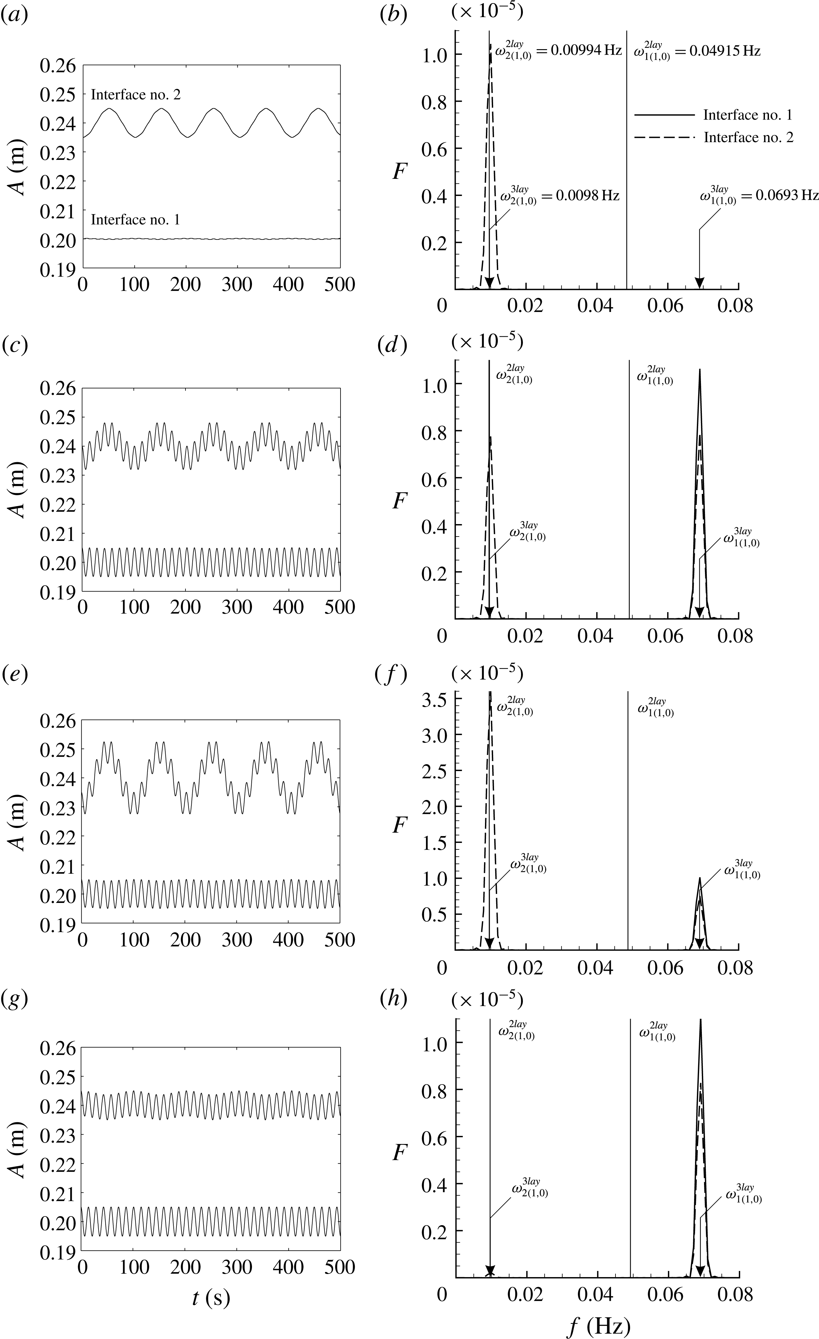
’ sign for the upper metal interface. The expression is similar to the coupled gravity wave solution in a 3 layer system considered in Horstmann et al. (Reference Horstmann, Weber and Weier2018). The physical meaning of the solutions (4.31) is best analysed by solving numerically the wave evolution equations (4.27), (4.28) to inspect specific initial perturbation effects on the two coupled interfaces. For this purpose the second-order implicit central finite difference scheme is used to approximate the time derivatives, see the appendix C. The physical variables are reconstructed using (4.7) and (4.8).
The results are shown as interface oscillations at the fixed position in the left corner of the cell shown in figure 1 (
 $x=0$
,
 $y=0$
) and the respective Fourier power spectra determined for different initial perturbation types:
 $(m,n)=\cos (m\unicode[STIX]{x03C0}/L_{x})+\cos (n\unicode[STIX]{x03C0}/L_{y})$
. The first analysed case is for the
 $\text{Mg}|\text{MgCl}_{2}{-}\text{KCl}{-}\text{NaCl}|\text{Sb}$
battery when
 $\unicode[STIX]{x1D70C}_{1}-\unicode[STIX]{x1D70C}_{2}\gg \unicode[STIX]{x1D70C}_{2}-\unicode[STIX]{x1D70C}_{3}$
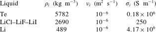
(the material physical properties are given in table 1), and the large scale rectangular cell with the dimensions:
 $L_{x}=8$
,
 $L_{y}=3.6$
m and the layer thicknesses:
 $h_{1}=0.2$
,
 $h_{2}=0.04$
,
 $h_{3}=0.2$
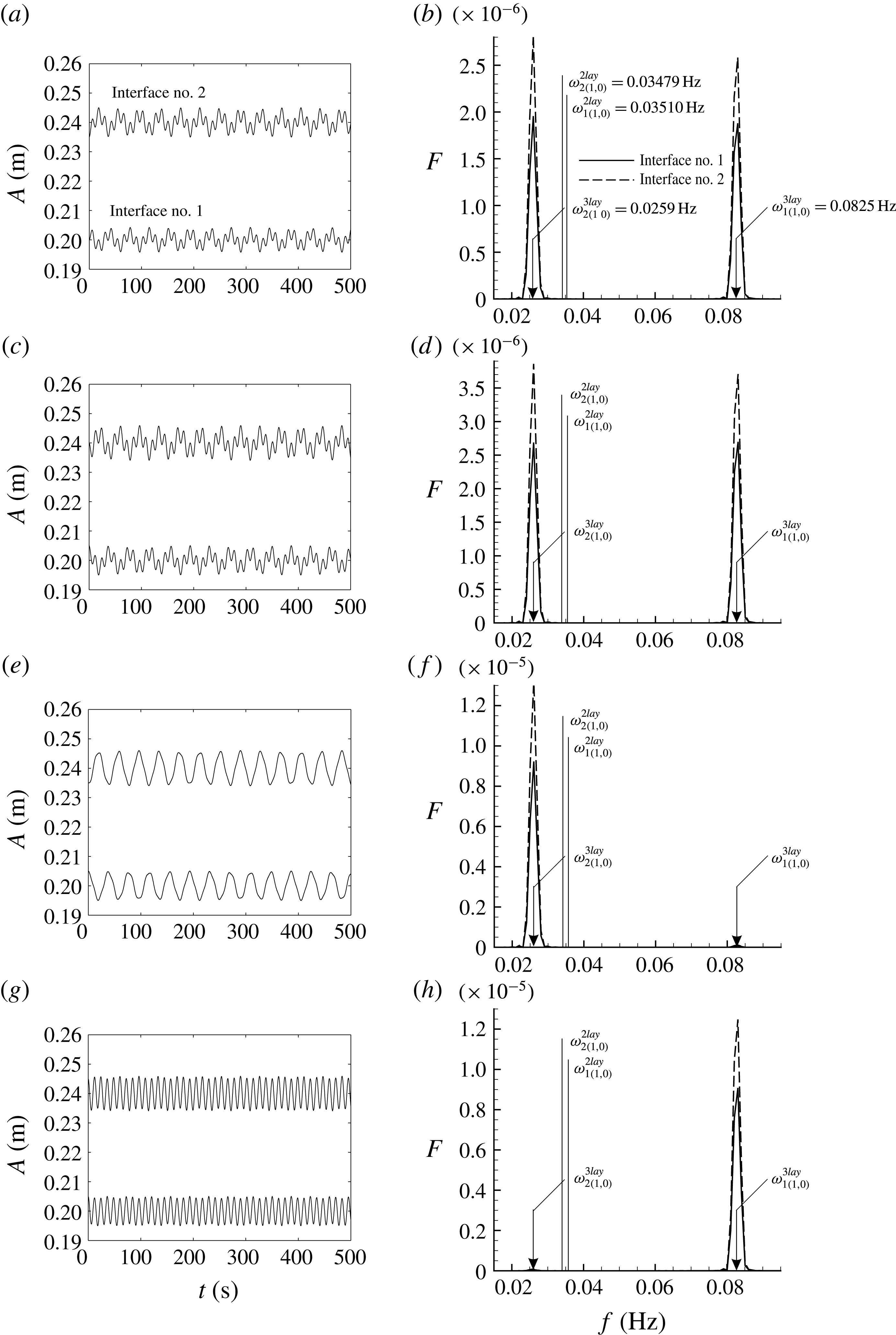
m. The obtained results are summarised in figure 2. If only the upper interface is initially perturbed at the amplitude
 $A=0.005$
m, using the single mode
 $m=1$
,
 $n=0$
, denoted as
 $(1,0)$
, and the lower interface is initially unperturbed, the initial value problem solution shows that there is only one peak in the spectra, see figure 2(a,b). This indicates that the lower interface remains practically motionless while the upper one is oscillating at the chosen initial perturbation frequency. In this example the 2 layer gravity frequencies: (4.17) and (4.18) can be compared to the 3 layer frequencies defined by (4.31). For the upper interface, the 2 and 3 layer approaches match quiet well
 $\unicode[STIX]{x1D714}_{2(1,0)}^{3lay}\approx \unicode[STIX]{x1D714}_{2(1,0)}^{2lay}$
.
However, this will not be the case for the lower interface for which
 $\unicode[STIX]{x1D714}_{1(1,0)}^{3lay}$
(4.31) is shifted towards higher frequencies compared to the
 $\unicode[STIX]{x1D714}_{1(1,0)}^{2lay}$
(4.17). In the following example shown in figure 2(c,d), when the lower interface is perturbed and the upper is initially unperturbed, a pair of the frequencies are excited in the system. The lower interface oscillates only at the frequency
 $\unicode[STIX]{x1D714}_{1(1,0)}^{3lay}(\neq \unicode[STIX]{x1D714}_{1(1,0)}^{2lay})$
. The spectrum of the upper interface consists of two peaks excited by the lower interface oscillation:
 $\unicode[STIX]{x1D714}_{1(1,0)}^{3lay}$
and
 $\unicode[STIX]{x1D714}_{2(1,0)}^{3lay}\approx \unicode[STIX]{x1D714}_{2(1,0)}^{2lay}$
.
Material parameters used in numerical examples: density
 $\unicode[STIX]{x1D70C}$
, kinematic viscosity
 $\unicode[STIX]{x1D708}$
, conductivity
 $\unicode[STIX]{x1D70E}$
of the three fluids comprising magnesium-based LMB (
 $\unicode[STIX]{x0394}\unicode[STIX]{x1D70C}_{1}\gg \unicode[STIX]{x0394}\unicode[STIX]{x1D70C}_{2}$
).

Solution for the 3 layer coupled gravity waves from the initial value problem with different perturbation types in the
 $\text{Mg}\Vert \text{Sb}$
battery: the left-hand side corresponds to the interface oscillations at the fixed position (
 $x=0$
,
 $y=0$
); the right-hand side shows the numerical Fourier power spectra compared to the analytical (4.17), (4.18) and (4.31): (a,b) only the top surface is perturbed initially; (c,d) only the bottom surface is perturbed; (e,f) both surfaces are perturbed asymmetrically at the initial moment; (g,h) both surfaces are perturbed symmetrically.
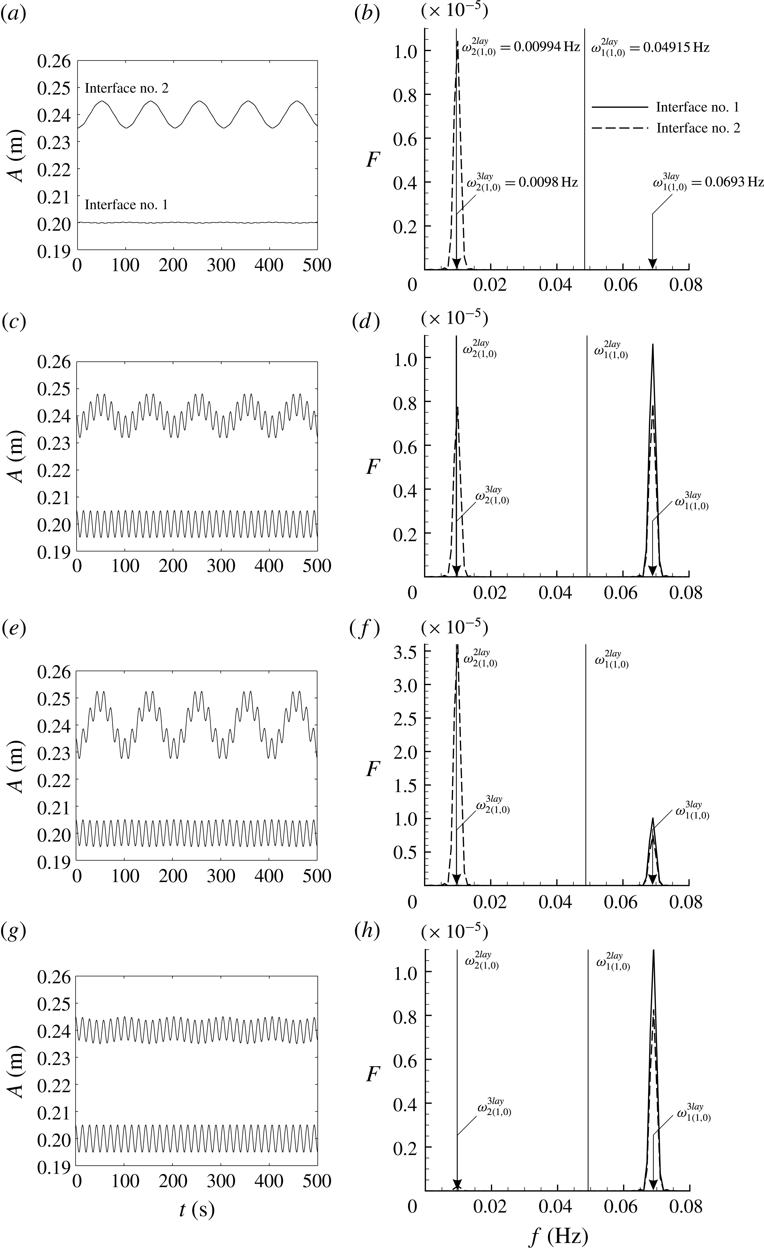
When both interfaces are initially perturbed in an asymmetric way (in opposite phase) in the
 $(1,0)$
modes of amplitudes
 $A=0.005$
m (see figure 2
g,h), the qualitative picture of the spectrum is similar to the previous case. The upper one contains a superposition of the two frequencies:
 $\unicode[STIX]{x1D714}_{1(1,0)}^{3lay}$
and
 $\unicode[STIX]{x1D714}_{2(1,0)}^{3lay}$
, whereas the lower oscillates at a single frequency:
 $\unicode[STIX]{x1D714}_{1(1,0)}^{3lay}$
.
When the two interfaces are initially perturbed in a symmetric way (in phase) at the respective
 $(1,0)$
modes, see figure 2(g,h), the wave response is quite different. The upper and lower metal interfaces oscillate at the single frequency:
 $\unicode[STIX]{x1D714}_{1(1,0)}^{3lay}$
.
From the above examples it can be concluded that the coupling of wave dynamics in the considered system is not symmetric. This is due to the significant density difference between the layers
 $\unicode[STIX]{x1D70C}_{1}-\unicode[STIX]{x1D70C}_{2}\gg \unicode[STIX]{x1D70C}_{2}-\unicode[STIX]{x1D70C}_{3}$
(similar results were obtained in direct numerical simulations by Weber et al. (Reference Weber, Beckstein, Herreman, Horstmann, Nore, Stefani and Weier2017)).
The excitation frequency response will be different if
 $\unicode[STIX]{x1D70C}_{1}-\unicode[STIX]{x1D70C}_{2}\approx \unicode[STIX]{x1D70C}_{2}-\unicode[STIX]{x1D70C}_{3}$
. To demonstrate this, an exotic battery case:
 $\text{Li}|\text{LiCl}{-}\text{LiF}{-}\text{LiI}|\text{Te}$
(Kim et al.
Reference Kim, Boysen, Newhouse, Spatocco, Chung, Burke, Bradwell, Jiang, Tomaszowska, Wang, Wei, Ortiz, Barriga, Poizeau and Sadoway2013) is considered (the material properties are given in table 2). The same system geometry and the perturbation strategy as in the previous examples is used. The obtained results are summarised in figure 3. If only the upper interface is initially perturbed and the lower interface is initially unperturbed, there are two frequency peaks observed on each of the interfaces, see figure 3(a,b). Both interfaces are set into the motion. Each interface oscillates at
 $\unicode[STIX]{x1D714}_{1(1,0)}^{3lay}\neq \unicode[STIX]{x1D714}_{1(1,0)}^{2lay}$
and
 $\unicode[STIX]{x1D714}_{2(1,0)}^{3lay}\neq \unicode[STIX]{x1D714}_{2(1,0)}^{2lay}$
. In this case
 $\unicode[STIX]{x1D714}_{1(1,0)}^{3lay}$
is shifted towards higher frequencies compared to
 $\unicode[STIX]{x1D714}_{1(1,0)}^{2lay}$
, and
 $\unicode[STIX]{x1D714}_{2(1,0)}^{3lay}$
is shifted towards lower frequencies compared to
 $\unicode[STIX]{x1D714}_{2(1,0)}^{2lay}$
.
In the following example (shown in figure 3
c,d), when the lower interface is perturbed and the upper is initially unperturbed, the situation is very similar to the previous example. Interfaces are oscillating at the two frequencies
 $\unicode[STIX]{x1D714}_{1(1,0)}^{3lay}$
and
 $\unicode[STIX]{x1D714}_{2(1,0)}^{3lay}$
.
Material parameters used in numerical examples: density
 $\unicode[STIX]{x1D70C}$
, kinematic viscosity
 $\unicode[STIX]{x1D708}$
, conductivity
 $\unicode[STIX]{x1D70E}$
of the three fluids comprising lithium-based LMB (
 $\unicode[STIX]{x0394}\unicode[STIX]{x1D70C}_{1}\approx \unicode[STIX]{x0394}\unicode[STIX]{x1D70C}_{2}$
).
When both interfaces are initially perturbed in the asymmetric way (opposite phase), see figure 3(e,f), the qualitative picture of the oscillations and the spectrum changes. The upper and lower interfaces oscillate at the single frequency, which is
 $\unicode[STIX]{x1D714}_{2(1,0)}^{3lay}$
, while the
 $\unicode[STIX]{x1D714}_{1(1,0)}^{3lay}$
vanishes from the spectrum.
When both interfaces are initially perturbed in symmetric way (in phase), see figure 3(g,h), the qualitative picture changes again. The upper and lower metal interface oscillates at the frequency
 $\unicode[STIX]{x1D714}_{1(1,0)}^{3lay}$
. In this case
 $\unicode[STIX]{x1D714}_{2(1,0)}^{3lay}$
is absent in the spectrum. Similar differences between the symmetric and asymmetric eigenvalue problem solution when
 $\unicode[STIX]{x1D70C}_{1}-\unicode[STIX]{x1D70C}_{2}\approx \unicode[STIX]{x1D70C}_{2}-\unicode[STIX]{x1D70C}_{3}$
were predicted in Horstmann et al. (Reference Horstmann, Weber and Weier2018) for the case of cylindrical cell.
Three layer coupled gravity waves as initial value problem for different perturbation cases for the
 $\text{Li}\Vert \text{Te}$
battery: the left-hand side corresponds to the interface oscillations at the fixed position (
 $x=0$
,
 $y=0$
); the right-hand side shows the Fourier power spectra: (a,b) only the top surface is perturbed; (c,d) only the bottom surface is perturbed; (e,f) both surfaces are perturbed asymmetrically; (g,h) both surfaces are perturbed symmetrically.
4.3 MHD eigenvalue problem
Let us proceed now with the stability analysis of the full MHD problem, taking into account the described coupling properties. For this purpose let us assume that the solution form is
 $\widetilde{\unicode[STIX]{x1D701}}_{i}\sim \text{e}^{\unicode[STIX]{x1D707}t}$
, where
 $\unicode[STIX]{x1D707}$
represents a set of complex eigenvalues.
 $\text{Re}(\unicode[STIX]{x1D707})$
represents the growth rate of instability (when
 $\text{Re}(\unicode[STIX]{x1D707})$
is positive the interfacial perturbation
 $\widetilde{\unicode[STIX]{x1D701}}$
starts to grow exponentially) and
 $\text{Im}(\unicode[STIX]{x1D707})$
is the electromagnetically modified gravitational wave frequency. The equations (4.27) and (4.28) lead to the following eigenvalue problem:
 $$\begin{eqnarray}\displaystyle (\unicode[STIX]{x1D63C}\unicode[STIX]{x1D707}^{2}+\unicode[STIX]{x1D63D}\unicode[STIX]{x1D707}+\unicode[STIX]{x1D63E})\boldsymbol{\cdot }\unicode[STIX]{x1D73B}=\mathbf{0}. & & \displaystyle\end{eqnarray}$$
The stability analysis is considerably simplified if restricted to a selected two mode interaction, similarly to Bojarevics & Romerio (Reference Bojarevics and Romerio1994), however accounting for the two interface coupling in the LMB case. Then from (4.27), (4.28) the two mode interaction results in:
 $$\begin{eqnarray}\displaystyle & \displaystyle \unicode[STIX]{x1D73B}=\left[\begin{array}{@{}c@{}}\widetilde{\unicode[STIX]{x1D701}}_{1,\boldsymbol{k}_{1}}\\ \widetilde{\unicode[STIX]{x1D701}}_{1,\boldsymbol{k}_{2}}\\ \widetilde{\unicode[STIX]{x1D701}}_{2,\boldsymbol{k}_{1}}\\ \widetilde{\unicode[STIX]{x1D701}}_{2,\boldsymbol{k}_{2}}\end{array}\right], & \displaystyle\end{eqnarray}$$
 $$\begin{eqnarray}\displaystyle & \displaystyle \unicode[STIX]{x1D63C}=\left[\begin{array}{@{}cccc@{}}1 & 0 & -R_{c,1} & 0\\ 0 & 1 & 0 & -R_{c,1}\\ -R_{c,2} & 0 & 1 & 0\\ 0 & -R_{c,2} & 0 & 1\end{array}\right], & \displaystyle\end{eqnarray}$$
 $$\begin{eqnarray}\displaystyle & \displaystyle \unicode[STIX]{x1D63D}=\left[\begin{array}{@{}cccc@{}}\unicode[STIX]{x1D6FE}_{1} & 0 & 0 & 0\\ 0 & \unicode[STIX]{x1D6FE}_{1} & 0 & 0\\ 0 & 0 & \unicode[STIX]{x1D6FE}_{2} & 0\\ 0 & 0 & 0 & \unicode[STIX]{x1D6FE}_{2}\end{array}\right], & \displaystyle\end{eqnarray}$$
 $$\begin{eqnarray}\displaystyle & \displaystyle \unicode[STIX]{x1D63E}=\left[\begin{array}{@{}cccc@{}}\unicode[STIX]{x1D714}_{1,\boldsymbol{k}_{1}}^{2} & \unicode[STIX]{x1D642}_{1,\boldsymbol{k}_{1},\boldsymbol{k}_{2}} & 0 & -\unicode[STIX]{x1D642}_{1,\boldsymbol{k}_{1},\boldsymbol{k}_{2}}\\ -\unicode[STIX]{x1D642}_{1,\boldsymbol{k}_{1},\boldsymbol{k}_{2}} & \unicode[STIX]{x1D714}_{1,\boldsymbol{k}_{2}}^{2} & \unicode[STIX]{x1D642}_{1,\boldsymbol{k}_{1},\boldsymbol{k}_{2}} & 0\\ 0 & -\unicode[STIX]{x1D642}_{2,\boldsymbol{k}_{1},\boldsymbol{k}_{2}} & \unicode[STIX]{x1D714}_{3,\boldsymbol{k}_{1}}^{2} & \unicode[STIX]{x1D642}_{2,\boldsymbol{k}_{1},\boldsymbol{k}_{2}}\\ -\unicode[STIX]{x1D642}_{2,\boldsymbol{k}_{1},\boldsymbol{k}_{2}}^{T} & 0 & \unicode[STIX]{x1D642}_{2,\boldsymbol{k}_{1},\boldsymbol{k}_{2}}^{T} & \unicode[STIX]{x1D714}_{3,\boldsymbol{k}_{2}}^{2}\end{array}\right]. & \displaystyle\end{eqnarray}$$
Let us consider an example when the applied magnetic field is constant
 $B_{z}$
, increasing at increments of
 $\unicode[STIX]{x0394}B=0.1$
mT from 0 to 3 mT, while the total applied current is fixed:
 $I=10^{5}$
A, and the dissipation is neglected (linear friction coefficients
 $\unicode[STIX]{x1D6FE}_{1}=\unicode[STIX]{x1D6FE}_{2}=0$
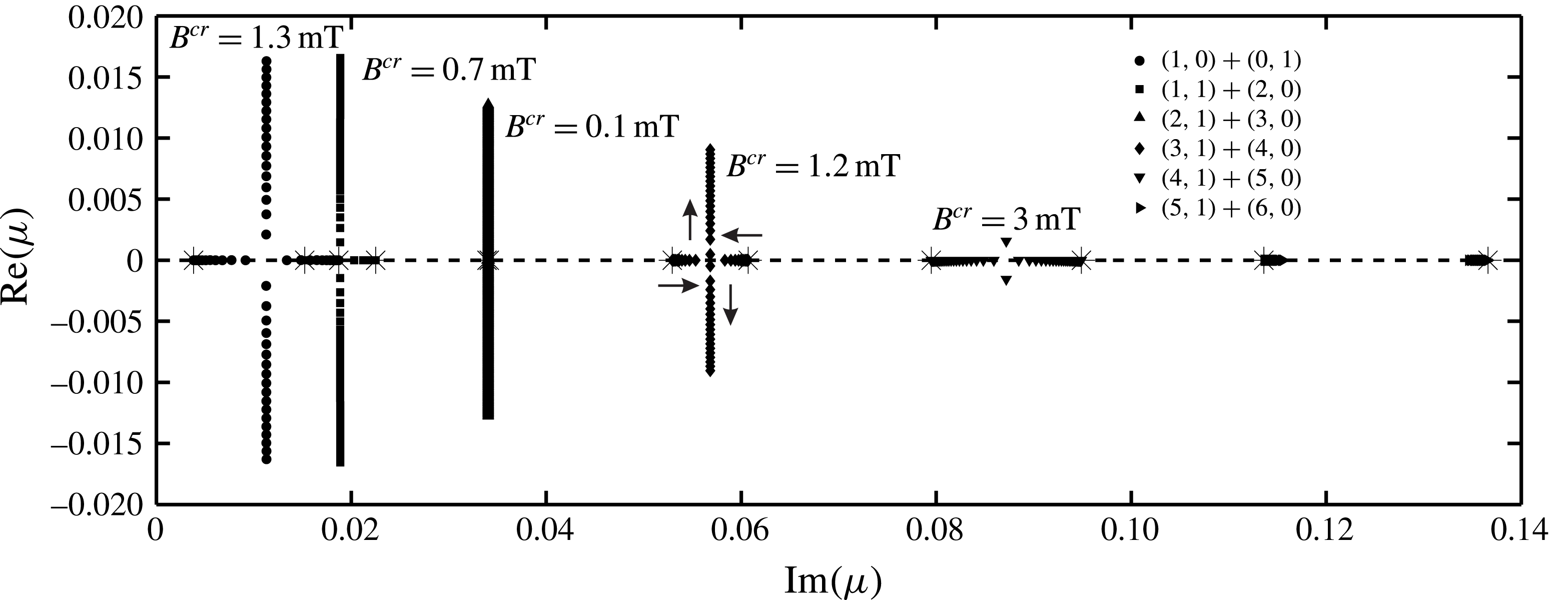
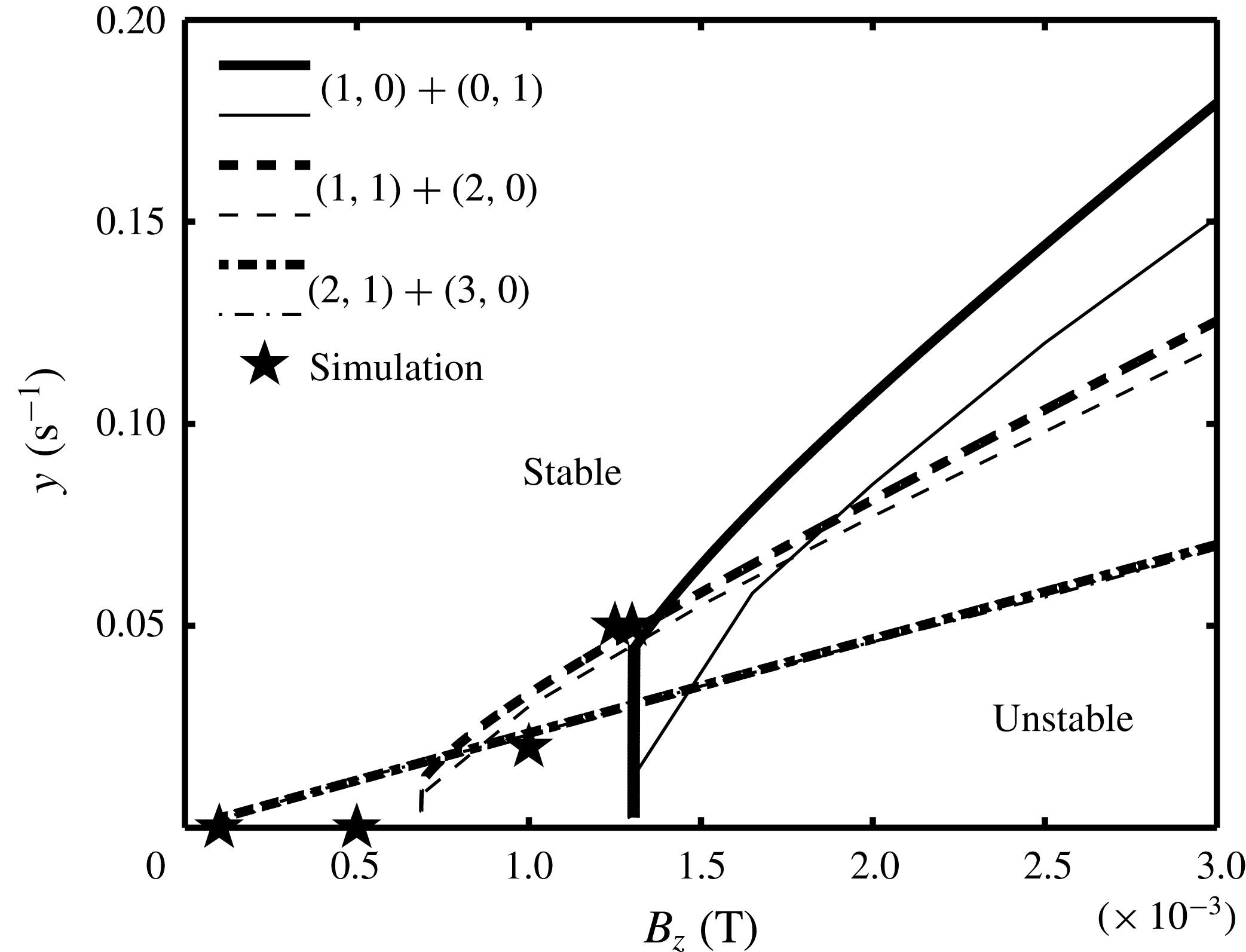
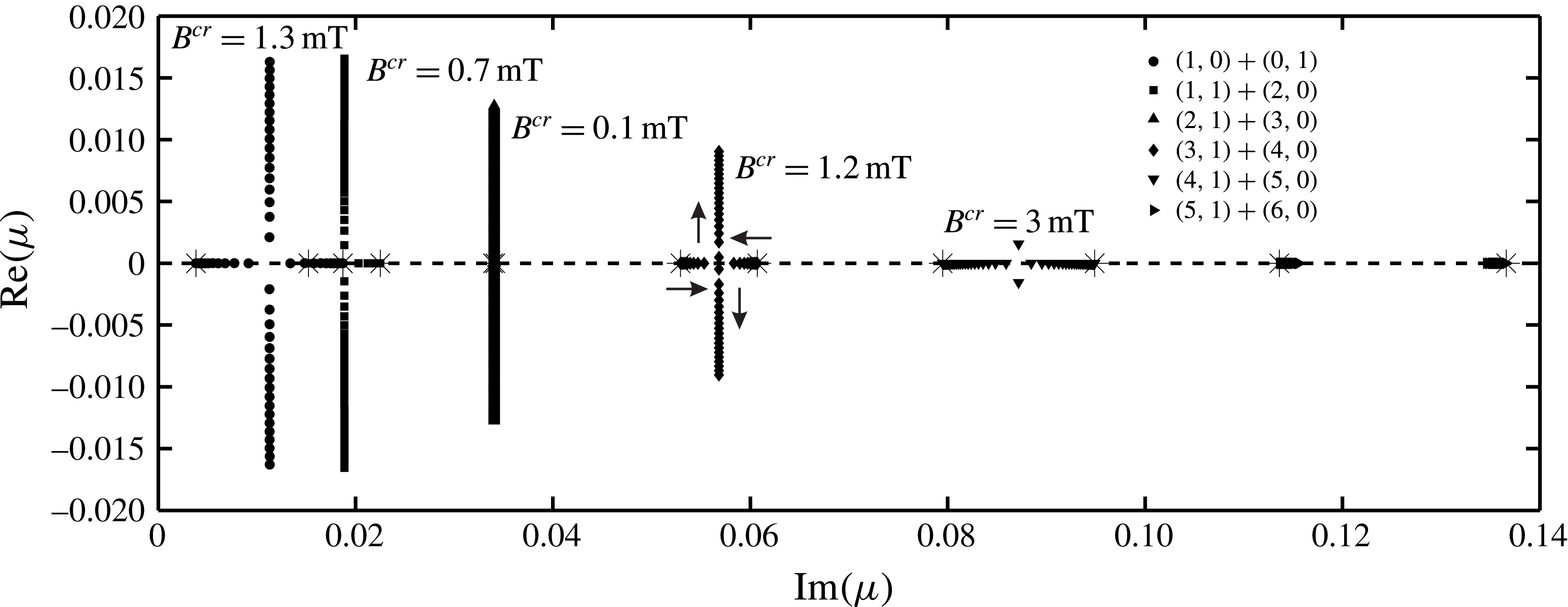
). The same cell geometry as in the § 4.2 and the material parameters from table 1 are used. Selected leading mode interactions for the upper interface are shown in figure 4. With the increase of magnetic field the frequencies of the interacting modes are shifted towards each other. When the critical
 $B^{cr}$
value is reached, the modes collide, followed by generation of a pair of complex-conjugate modes. One of these gives a positive growth increment that leads to the system destabilisation. The results for various mode interactions show that the most dangerous growth rates are for the modes
 $(1,0)+(0,1)$
;
 $(1,1)+(2,0)$
and
 $(2,1)+(3,0)$
. In § 4.6, these findings will be compared with the HHC numerical model (Bojarevics & Evans Reference Bojarevics and Evans2015). In general, the larger the interacting mode wavenumber, the larger the critical magnetic field value at which they collide (figure 4). As expected, for the lower interface all the basic mode interactions in the considered magnetic field range remain stable due to the large density difference of the lower metal and the electrolyte (
 $\text{Mg}\Vert \text{Sb}$
case). The critical magnetic field is determined by the top interface instability.
Eigenvalue analysis for the upper interface: selected eigenvalue couples are moving with the incremental rise of magnetic field
 $B_{z}=B_{z}^{0}+\unicode[STIX]{x0394}B$
, where
 $0\leqslant B_{z}\leqslant 3$
mT,
 $\unicode[STIX]{x0394}B=0.1$
mT,
 $L_{x}/L_{y}=2.2$
; the initial
 $B_{z}=0$
position is marked by star signs (
 $\ast$
) and the value of
 $B^{cr}$
is shown for each interaction.
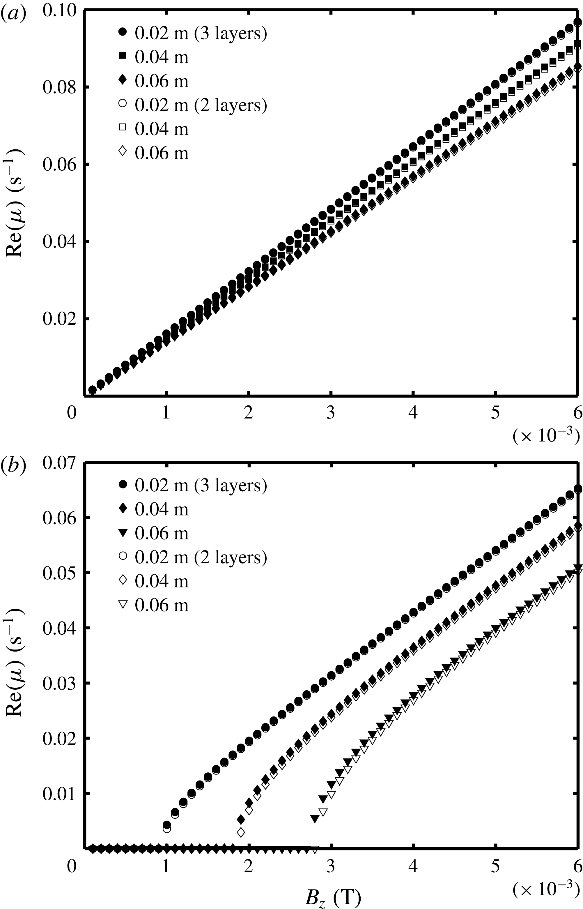
Comparison of the growth increment dependency on applied magnetic field for the 2 layer and 3 layer models for various values of the electrolyte thickness for
 $L_{x}/L_{y}=1$
: (a) the mode
 $(1,0)+(0,1)$
interaction; (b)
 $(1,1)+(2,0)$
interaction.

When analysing the impact of cell aspect ratio, for instance,
 $L_{x}/L_{y}=1;2;2.5$
etc., the obtained results for interacting modes are in agreement with the results in Munger & Vincent (Reference Munger and Vincent2008) obtained for the HHC case when the top metal layer stability is dominant in the LMB case.
4.4 The square cell case
The previous examples demonstrate that some unperturbed gravity wave mode frequencies are very close in value, however at relatively higher mode orders. In the presence of dissipation these will be damped more rapidly than the leading modes
 $(1,0)$
and
 $(0,1)$
. In a special case, when the cell aspect ratio
 $L_{x}/L_{y}=1$
, the square horizontal section cell is expected to be the most unstable case. The following results are not dependent on the magnitude of the
 $L_{x}$
,
 $L_{y}$
as long as the
 $\unicode[STIX]{x1D6FF}$
parameters is sufficiently low to validate the shallow layer approximation. If keeping the same material properties (
 $\text{Mg}\Vert \text{Sb}$
), total current and the unperturbed current density as in the previous large scale cell examples, the square cell will have the dimensions
 $L_{x}=L_{y}=5.37$
m. Figure 5 shows a comparison of the growth increment dependency on the depth of electrolyte for the linear stability cases of coupled three layers and the two top layers only. As can be seen from figure 5, the full three layer model is just marginally different to the two layer model. As previously, we restrict attention to the typical two mode interactions to gain insight to the specific mode interaction mechanisms.
As expected, for the square cell the
 $(1,0)+(0,1)$
interaction becomes unstable at the smallest magnetic field values for all considered electrolyte depth values. The same result is obtained if reducing the
 $L_{x}$
and
 $L_{y}$
value down to 0.2 m and the typical electric current
 $I\approx 130$
A, used in the small scale experimental set-up. In the case of
 $(1,1)+(2,0)$
mode interaction the stability is retained until a critical magnetic field is reached (at approximately 1 mT for
 $h_{2}=0.02$
m). The stability of the latter interaction increases with the thickness of the electrolyte. The high sensitivity of square cells to the vertical magnetic field is confirmed by Zikanov (Reference Zikanov2018) using the numerical fully coupled nonlinear model based on the shallow layer approximation.
4.5 Stability criteria with friction effect
The effect of bottom friction on the gravity wave damping is analysed in Landau & Lifshitz (Reference Landau, Lifshitz, Sykes and Reid1987, p. 93) for laminar flow. In reality the friction coefficient values in (4.27), (4.28) could be significantly higher due to the surface roughness and turbulence generated by the horizontal recirculation flow due to the rotational part of the electromagnetic force in the fluid. The numerical models for aluminium electrolysis cells typically invoke additional turbulence models and empirical values for the bottom friction coefficients, see Bojarevics & Evans (Reference Bojarevics and Evans2015). The present linear theory can be used to obtain some analytical estimates of the stability criteria for the liquid metal battery MHD waves when the top and bottom friction coefficients are included.
In the previous sections it was demonstrated that the upper interface stability is the most critical, therefore we will simplify the derivation by restricting to the equation for the
 $\unicode[STIX]{x1D701}_{2}$
interface. This derivation extends the previous results by adding the effects of friction, while maintaining the electric current redistribution due to the lower metal layer. Based on the assumption that the lower metal is at significantly higher density (
 $\unicode[STIX]{x1D70C}_{1}\gg \unicode[STIX]{x1D70C}_{3}$
,
 $\unicode[STIX]{x1D701}_{1}\rightarrow 0$
), the wave equation for the upper interface is
 $$\begin{eqnarray}\displaystyle \unicode[STIX]{x2202}_{tt}\widetilde{\unicode[STIX]{x1D701}}_{\boldsymbol{k}}+\unicode[STIX]{x1D6FE}\unicode[STIX]{x2202}_{t}\widetilde{\unicode[STIX]{x1D701}}_{\boldsymbol{k}}+\unicode[STIX]{x1D714}_{\boldsymbol{k}}^{2}\widetilde{\unicode[STIX]{x1D701}}_{\boldsymbol{k}}=\mathop{\sum }_{\boldsymbol{k}^{\prime }\geqslant 0}\unicode[STIX]{x1D642}_{\boldsymbol{k},\boldsymbol{k}^{\prime }}\widetilde{\unicode[STIX]{x1D701}}_{\boldsymbol{k}^{\prime }}. & & \displaystyle\end{eqnarray}$$
Taking into account that
 $(h_{1}h_{2}\boldsymbol{k}^{2}+\unicode[STIX]{x1D70E}_{e,1})\approx (h_{2}h_{3}\boldsymbol{k}^{2}+\unicode[STIX]{x1D70E}_{e,2})$
(4.30) reduces to:
 $$\begin{eqnarray}\displaystyle \unicode[STIX]{x1D642}_{\boldsymbol{k},\boldsymbol{k}^{\prime }} & = & \displaystyle -\frac{j}{4\unicode[STIX]{x1D6FC}_{2}}\unicode[STIX]{x1D716}_{\boldsymbol{k}}\unicode[STIX]{x1D716}_{\boldsymbol{k}^{\prime }}[(k_{y}^{\prime }k_{x}-k_{x}^{\prime }k_{y})(\widehat{B}_{k_{x}^{\prime }-k_{x},k_{y}^{\prime }-k_{y}}-\widehat{B}_{k_{x}^{\prime }+k_{x},k_{y}^{\prime }+k_{y}})\nonumber\\ \displaystyle & & \displaystyle +\,(k_{y}^{\prime }k_{x}+k_{x}^{\prime }k_{y})(\widehat{B}_{k_{x}^{\prime }-k_{x},k_{y}^{\prime }+k_{y}}-\widehat{B}_{k_{x}^{\prime }+k_{x},k_{y}^{\prime }-k_{y}})]\nonumber\\ \displaystyle & & \displaystyle \times \,(h_{2}h_{3}\boldsymbol{k}^{2}+\unicode[STIX]{x1D70E}_{e,2})^{-1/2}(h_{2}h_{3}\boldsymbol{k}^{\prime 2}+\unicode[STIX]{x1D70E}_{e,2})^{-1/2}.\end{eqnarray}$$
The solution of the eigenvalue problem, when two mode interaction stability is considered, can be reduced to a dispersion relation of the fourth order, that can be written as
 $$\begin{eqnarray}\displaystyle \mathop{\sum }_{l=0}^{4}a_{l}\unicode[STIX]{x1D707}^{l}=0, & & \displaystyle\end{eqnarray}$$
where
 $$\begin{eqnarray}\displaystyle a_{0}=\unicode[STIX]{x1D714}_{\boldsymbol{k}_{1}}^{2}\unicode[STIX]{x1D714}_{\boldsymbol{k}_{2}}^{2}+|\unicode[STIX]{x1D642}_{\boldsymbol{k}_{1},\boldsymbol{k}_{2}}|^{2},\quad a_{1}=\unicode[STIX]{x1D714}_{\boldsymbol{k}_{1}}^{2}+\unicode[STIX]{x1D714}_{\boldsymbol{k}_{2}}^{2},\quad a_{2}=\unicode[STIX]{x1D714}_{\boldsymbol{k}_{1}}^{2}+\unicode[STIX]{x1D714}_{\boldsymbol{k}_{2}}^{2}+\unicode[STIX]{x1D6FE}^{2},\quad a_{3}=2\unicode[STIX]{x1D6FE},\quad a_{4}=1. & & \displaystyle \nonumber\\ \displaystyle & & \displaystyle\end{eqnarray}$$
The explicit solution can be obtained for the selected
 $\boldsymbol{k}_{1}$
and
 $\boldsymbol{k}_{2}$
mode interaction:
 $$\begin{eqnarray}\displaystyle \unicode[STIX]{x1D707}=-\frac{\unicode[STIX]{x1D6FE}}{2}\pm (\unicode[STIX]{x1D6E4}_{\boldsymbol{k}_{1}\boldsymbol{k}_{2}}+(\unicode[STIX]{x1D6E5}_{\boldsymbol{k}_{1}\boldsymbol{k}_{2}}^{2})^{1/2})^{1/2}, & & \displaystyle\end{eqnarray}$$
where
 $$\begin{eqnarray}\displaystyle \unicode[STIX]{x1D6E4}_{\boldsymbol{k}_{1}\boldsymbol{k}_{2}}=\frac{\unicode[STIX]{x1D6FE}^{2}}{4}-\unicode[STIX]{x1D6FA}_{\boldsymbol{k}_{1}\boldsymbol{k}_{2}}^{2},\quad \unicode[STIX]{x1D6FA}_{\boldsymbol{k}_{1}\boldsymbol{k}_{2}}^{2}=\frac{\unicode[STIX]{x1D714}_{\boldsymbol{k}_{1}}^{2}+\unicode[STIX]{x1D714}_{\boldsymbol{ k}_{2}}^{2}}{2},\quad \unicode[STIX]{x1D6E5}_{\boldsymbol{k}_{1}\boldsymbol{k}_{2}}^{2}=\left(\frac{\unicode[STIX]{x1D714}_{\boldsymbol{k}_{1}}^{2}-\unicode[STIX]{x1D714}_{\boldsymbol{ k}_{2}}^{2}}{2}\right)^{2}-|\unicode[STIX]{x1D642}_{\boldsymbol{ k}_{1},\boldsymbol{k}_{2}}|^{2}. & & \displaystyle \nonumber\\ \displaystyle & & \displaystyle\end{eqnarray}$$
In the frictionless case (
 $\unicode[STIX]{x1D6FE}=0$
) the sufficient condition for the instability is
 $$\begin{eqnarray}\displaystyle \unicode[STIX]{x1D6E5}_{\boldsymbol{k}_{1}\boldsymbol{k}_{2}}^{2}\leqslant 0. & & \displaystyle\end{eqnarray}$$
If the stability is reached at a finite
 $\unicode[STIX]{x1D6FE}$
, then
 $\text{Re}(\unicode[STIX]{x1D707})>0$
and (4.41) rewrites as
 $$\begin{eqnarray}\displaystyle \unicode[STIX]{x1D707}=-\frac{\unicode[STIX]{x1D6FE}}{2}\pm (\unicode[STIX]{x1D6E4}_{\boldsymbol{k}_{1}\boldsymbol{k}_{2}}\pm \text{i}|\unicode[STIX]{x1D6E5}_{\boldsymbol{k}_{1}\boldsymbol{k}_{2}}|)^{1/2}. & & \displaystyle\end{eqnarray}$$
In the case when the system is slightly above the instability threshold (
 $|\unicode[STIX]{x1D6E5}_{\boldsymbol{k}_{1}\boldsymbol{k}_{2}}|\rightarrow 0$
), the square root in (4.44) can be expanded in Taylor series, to find the fastest growing mode:
 $$\begin{eqnarray}\displaystyle \unicode[STIX]{x1D707}=-\frac{\unicode[STIX]{x1D6FE}}{2}+\unicode[STIX]{x1D6E4}_{\boldsymbol{k}_{1}\boldsymbol{k}_{2}}^{1/2}+\frac{1}{2}\unicode[STIX]{x1D6E4}_{\boldsymbol{k}_{1}\boldsymbol{k}_{2}}^{-1/2}\text{i}|\unicode[STIX]{x1D6E5}_{\boldsymbol{k}_{1}\boldsymbol{k}_{2}}|+O(|\unicode[STIX]{x1D6E5}_{\boldsymbol{k}_{1}\boldsymbol{k}_{2}}|^{2}). & & \displaystyle\end{eqnarray}$$
For a small friction (
 $\unicode[STIX]{x1D6FE}\rightarrow 0$
) (4.45) reduces to:
 $$\begin{eqnarray}\displaystyle \unicode[STIX]{x1D707}=-\frac{\unicode[STIX]{x1D6FE}}{2}+\text{i}\unicode[STIX]{x1D6FA}_{\boldsymbol{k}_{1}\boldsymbol{k}_{2}}+\frac{|\unicode[STIX]{x1D6E5}_{\boldsymbol{k}_{1}\boldsymbol{k}_{2}}|}{2\unicode[STIX]{x1D6FA}_{\boldsymbol{k}_{1}\boldsymbol{k}_{2}}}. & & \displaystyle\end{eqnarray}$$
The system will be unstable if
 $\text{Re}(\unicode[STIX]{x1D707})\geqslant 0$
, meaning that the friction coefficient
 $$\begin{eqnarray}\displaystyle \unicode[STIX]{x1D6FE}\leqslant \frac{|\unicode[STIX]{x1D6E5}_{\boldsymbol{k}_{1}\boldsymbol{k}_{2}}|}{\unicode[STIX]{x1D6FA}_{\boldsymbol{k}_{1}\boldsymbol{k}_{2}}}. & & \displaystyle\end{eqnarray}$$
The explicit criterion for the instability is
 $$\begin{eqnarray}\displaystyle \unicode[STIX]{x1D6FE}\leqslant \left(\frac{2}{\unicode[STIX]{x1D714}_{\boldsymbol{k}_{1}}^{2}+\unicode[STIX]{x1D714}_{\boldsymbol{k}_{2}}^{2}}\right)^{1/2}\left(|\unicode[STIX]{x1D642}_{\boldsymbol{k}_{1},\boldsymbol{k}_{2}}|^{2}-\left(\frac{\unicode[STIX]{x1D714}_{\boldsymbol{k}_{1}}^{2}-\unicode[STIX]{x1D714}_{\boldsymbol{ k}_{2}}^{2}}{2}\right)^{2}\right)^{1/2}. & & \displaystyle\end{eqnarray}$$
Alternatively the stability condition (4.48) can be derived by applying the Routh–Hurwitz (Gantmacher Reference Gantmacher and Brenner1959, p. 231) criterion to (4.39), giving the same expression as (4.48).
If the considered modes
 $\boldsymbol{k}_{1}$
and
 $\boldsymbol{k}_{2}$
are close enough (
 $\text{Im}(\unicode[STIX]{x1D707}_{1})\rightarrow \text{Im}(\unicode[STIX]{x1D707}_{2})$
) then (4.48) reduces to
 $$\begin{eqnarray}\displaystyle \unicode[STIX]{x1D6FE}\leqslant \left(\frac{2}{\unicode[STIX]{x1D714}_{\boldsymbol{k}_{1}}^{2}+\unicode[STIX]{x1D714}_{\boldsymbol{k}_{2}}^{2}}\right)^{1/2}|\unicode[STIX]{x1D642}_{\boldsymbol{k}_{1},\boldsymbol{k}_{2}}|. & & \displaystyle\end{eqnarray}$$
The results correlating the critical magnetic field
 $B_{z}$
and the friction coefficient
 $\unicode[STIX]{x1D6FE}$
are depicted in figure 6. The same cell geometry as in § 4.2 and the material parameters from table 1 are used for the total electric current
 $I=10^{5}$
A. The results show that the asymptotic relation (4.48) gives a good approximation to the general expression (4.41). The relation (4.48) gives the result which is the same as that obtained if using the numerical
 $QZ$
algorithm from the standard, linear algebra software library LAPACK (Anderson et al.
Reference Andreson, Bai, Bischof, Blackford, Demmel, Dongarra, Du Croz, Greenbaum, Hammarling, McKenney and Sorensen1999), except in the case of
 $(1,0)$
,
 $(0,1)$
interaction with a relatively large gap between the unperturbed gravity frequencies (figure 4). Note that the discontinuity of stabilising friction dependency on the magnetic field appears due to the critical magnetic field threshold, below which the system will be always in stable state in the inviscid limit.
It is instructive to present the general criterion (4.48) in the explicit form for the basic
 $(1,0)$
and
 $(0,1)$
mode interaction stability threshold criterion:
 $$\begin{eqnarray}\displaystyle \unicode[STIX]{x1D6FE}\leqslant \left[\frac{128j^{2}B_{z}^{02}}{(\unicode[STIX]{x1D70C}_{2}/h_{2}+\unicode[STIX]{x1D70C}_{3}/h_{3})(\unicode[STIX]{x1D70C}_{2}-\unicode[STIX]{x1D70C}_{3})g\unicode[STIX]{x03C0}^{6}h_{2}^{2}h_{3}^{2}}\frac{L_{x}^{2}L_{y}^{2}}{L_{x}^{2}+L_{y}^{2}}-\frac{(\unicode[STIX]{x1D70C}_{2}-\unicode[STIX]{x1D70C}_{3})g\unicode[STIX]{x03C0}^{2}}{2(\unicode[STIX]{x1D70C}_{2}/h_{2}+\unicode[STIX]{x1D70C}_{3}/h_{3})}\frac{(L_{y}^{2}-L_{x}^{2})^{2}}{L_{x}^{2}L_{y}^{2}(L_{x}^{2}+L_{y}^{2})}\right]^{1/2}. & & \displaystyle \nonumber\\ \displaystyle & & \displaystyle\end{eqnarray}$$
In the frictionless case (
 $\unicode[STIX]{x1D6FE}=0$
) the stability condition (4.50) by Bojarevics & Romerio (Reference Bojarevics and Romerio1994) is recovered:
 $$\begin{eqnarray}\displaystyle (\unicode[STIX]{x1D70C}_{2}-\unicode[STIX]{x1D70C}_{3})g\unicode[STIX]{x03C0}^{4}h_{2}h_{3}\left(\frac{1}{L_{y}^{2}}-\frac{1}{L_{x}^{2}}\right)=16jB_{z}^{0}. & & \displaystyle\end{eqnarray}$$
The oscillation frequency at the instability onset is defined by (4.42):
 $\unicode[STIX]{x1D6FA}_{\boldsymbol{k}_{1}\boldsymbol{k}_{2}}=\sqrt{(\unicode[STIX]{x1D714}_{\boldsymbol{k}_{1}}^{2}+\unicode[STIX]{x1D714}_{\boldsymbol{k}_{2}}^{2})/2}$
, which is the root-mean-square (r.m.s.) value of the two interacting gravity modes and can be measured experimentally.

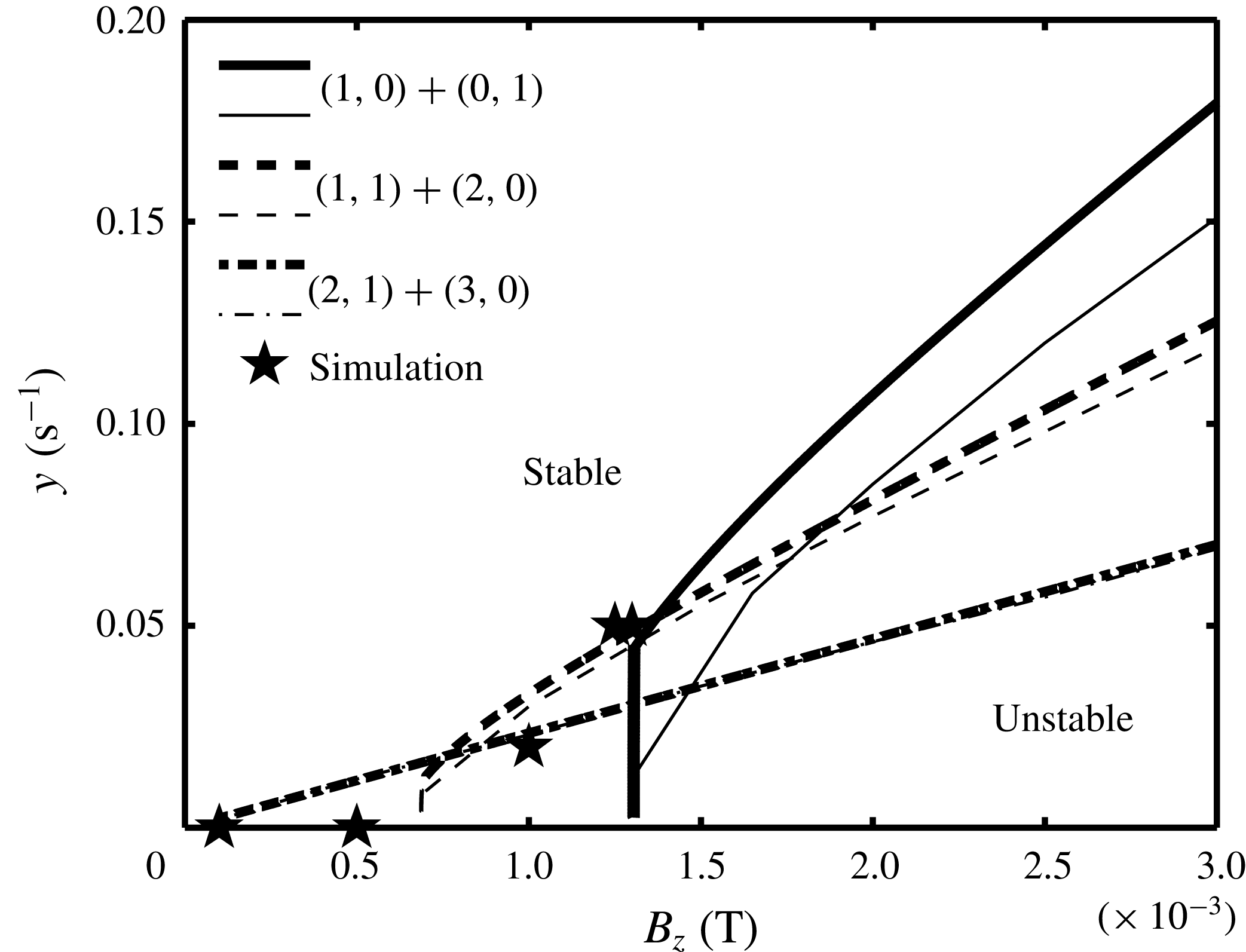
4.6 Numerical examples
In order to demonstrate the validity of the 2 layer approximation versus the 3 layer approximation of the batteries for a selection of materials (the properties given in Horstmann et al. (Reference Horstmann, Weber and Weier2018)) the fully coupled numerical model was solved using (2.25)–(2.28) taking into account the nonlinear wave velocity terms at the right-hand side (see appendix C). The electric current redistribution was obtained by solving (4.21)–(4.22). The full 3 layer coupled solutions were compared to the uncoupled 2 layer numerical solutions and the 3 layer respective linear stability results for the same cell geometry as in § 4.2, when the total applied current is fixed at
 $I=10^{5}$
A while the dissipation is neglected (
 $\unicode[STIX]{x1D6FE}_{1}=\unicode[STIX]{x1D6FE}_{2}=0$
).
The importance of the ratio of the density differences
 $(\unicode[STIX]{x1D70C}_{1}-\unicode[STIX]{x1D70C}_{2})/(\unicode[STIX]{x1D70C}_{2}-\unicode[STIX]{x1D70C}_{3})$
for the purely hydrodynamic wave coupling was emphasised by Horstmann et al. (Reference Horstmann, Weber and Weier2018). The critical magnetic field dependency on this parameter can be analysed using the MHD theory developed in the present paper when neglecting the effects of dissipation. The following approximations were compared:
(i) linear stability for the 2 layer case;
(ii) linear stability for 3 layers;
(iii) decoupled 2 interface simulation;
(iv) fully coupled 3 layer simulation.
The obtained results are summarised in figure 7. Overall a relatively good agreement between all approximations can be seen for the majority of material combinations. The maximum difference for the predicted
 $B^{cr}$
relative to the fully coupled 3 layer simulation is less than 18 %. In the range
 $1<(\unicode[STIX]{x1D70C}_{1}-\unicode[STIX]{x1D70C}_{2})/(\unicode[STIX]{x1D70C}_{2}-\unicode[STIX]{x1D70C}_{3})<5$
the 2 layer linear stability overestimates the critical magnetic field, while the decoupled 2 interface simulation underestimates it. In this range the 3 layer linear stability underestimates the system stability if compared to the fully coupled solution.
Critical stability comparison for different battery compositions: (▪) linear stability for the 2 layers, (●) linear stability for the 3 layers, (▲) decoupled 2 interface simulation, (♦) fully coupled 3 layer simulation. (1)
 $\text{Li}\Vert \text{Te}$
, (2)
 $\text{Na}\Vert \text{Sn}$
, (3)
 $\text{Li}\Vert \text{Bi}$
, (4)
 $\text{Li}\Vert \text{Pb}$
, (5)
 $\text{Na}\Vert \text{Bi}$
,
 $\text{Na}\Vert \text{Pb}$
, (6)
 $\text{Li}\Vert \text{Zn}$
, (7)
 $\text{Li}\Vert \text{Sn}$
, (8)
 $\text{Ca}\Vert \text{Sb}$
, (9)
 $\text{Ca}\Vert \text{Bi}$
, (10)
 $\text{Mg}\Vert \text{Sb}$
.
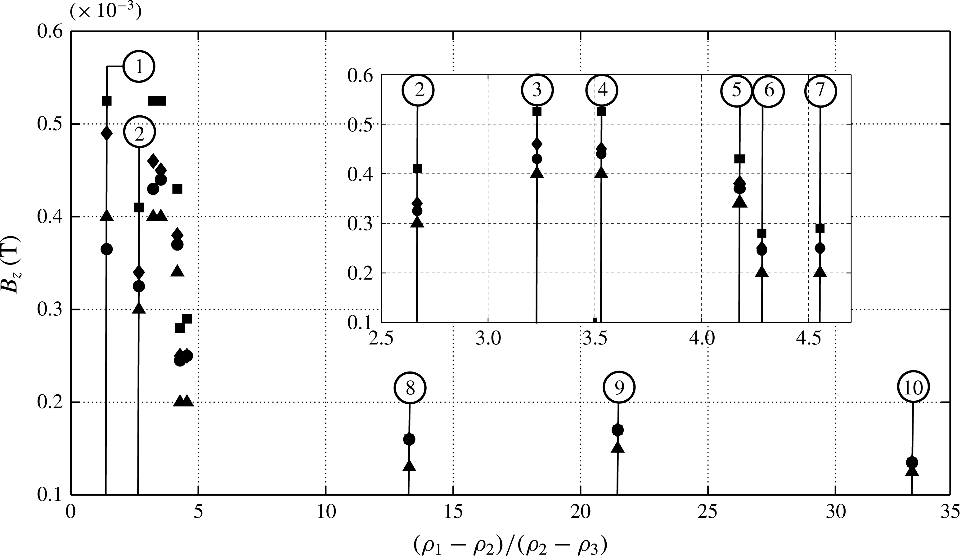
The largest difference to fully coupled 3 layer simulation is reached when
 $(\unicode[STIX]{x1D70C}_{1}-\unicode[STIX]{x1D70C}_{2})/(\unicode[STIX]{x1D70C}_{2}-\unicode[STIX]{x1D70C}_{3})\approx 1$
, which corresponds, e.g. to the
 $\text{Li}\Vert \text{Te}$
battery case. For this material combination the 3 layer linear stability predicts the critical magnetic field value 0.365 mT and the fully coupled approach gives
 $B^{cr}=0.49$
mT, respectively.
The lowest critical magnetic field value is found for the
 $\text{Mg}\Vert \text{Sb}$
battery, which emphasises the importance of the interfacial stability for this material combination. In this case both the 2 and 3 layer linear stability predict
 $B^{cr}=0.135$
mT. The numerical simulation for the decoupled two interfaces gives 0.125 mT and the fully coupled case results in 0.135 mT critical value respectively. According to figure 6, the instability develops at the low value of
 $B_{z}$
due to the closely located modes
 $(2,1)+(3,0)$
.
Generally with the decrease of the density ratio,
 $(\unicode[STIX]{x1D70C}_{1}-\unicode[STIX]{x1D70C}_{2})/(\unicode[STIX]{x1D70C}_{2}-\unicode[STIX]{x1D70C}_{3})$
, all four approximations predict gradual increase of the critical magnetic field value due to the increased density difference between the upper metal and the electrolyte:
 $\unicode[STIX]{x1D70C}_{2}-\unicode[STIX]{x1D70C}_{3}$
. For the particular case of
 $\text{Na}\Vert \text{Sn}$
battery a drop of the critical magnetic field is observed due to the lower density difference between the electrolyte and the upper metal (
 $\unicode[STIX]{x1D70C}_{2}-\unicode[STIX]{x1D70C}_{3}=1619~\text{kg}~\text{m}^{-3}$
) if compared to the density differences for
 $\text{Li}\Vert \text{Te}$
and
 $\text{Li}\Vert \text{Bi}$
, which are 2201 and
 $2202~\text{kg}~\text{m}^{-3}$
respectively.
Numerical results for the top interface oscillation following the initial
 $(1,0)$
mode perturbation at
 $A=0.005$
m: (a) oscillation in the frictionless case (
 $\unicode[STIX]{x1D6FE}=0$
) for subcritical and overcritical magnetic fields, (b) the power spectra for
 $\unicode[STIX]{x1D6FE}=0$
cases, the black vertical continuous lines mark the gravity wave frequencies, (c) oscillation in the presence of friction, (d) the power spectra for the two friction coefficients at the marginally stable and unstable cases, (e) oscillation at the higher friction (
 $\unicode[STIX]{x1D6FE}=0.05~\text{s}^{-1}$
) for
 $B_{z}$
near the stability limit, (f) the spectral peaks near the stability limit.
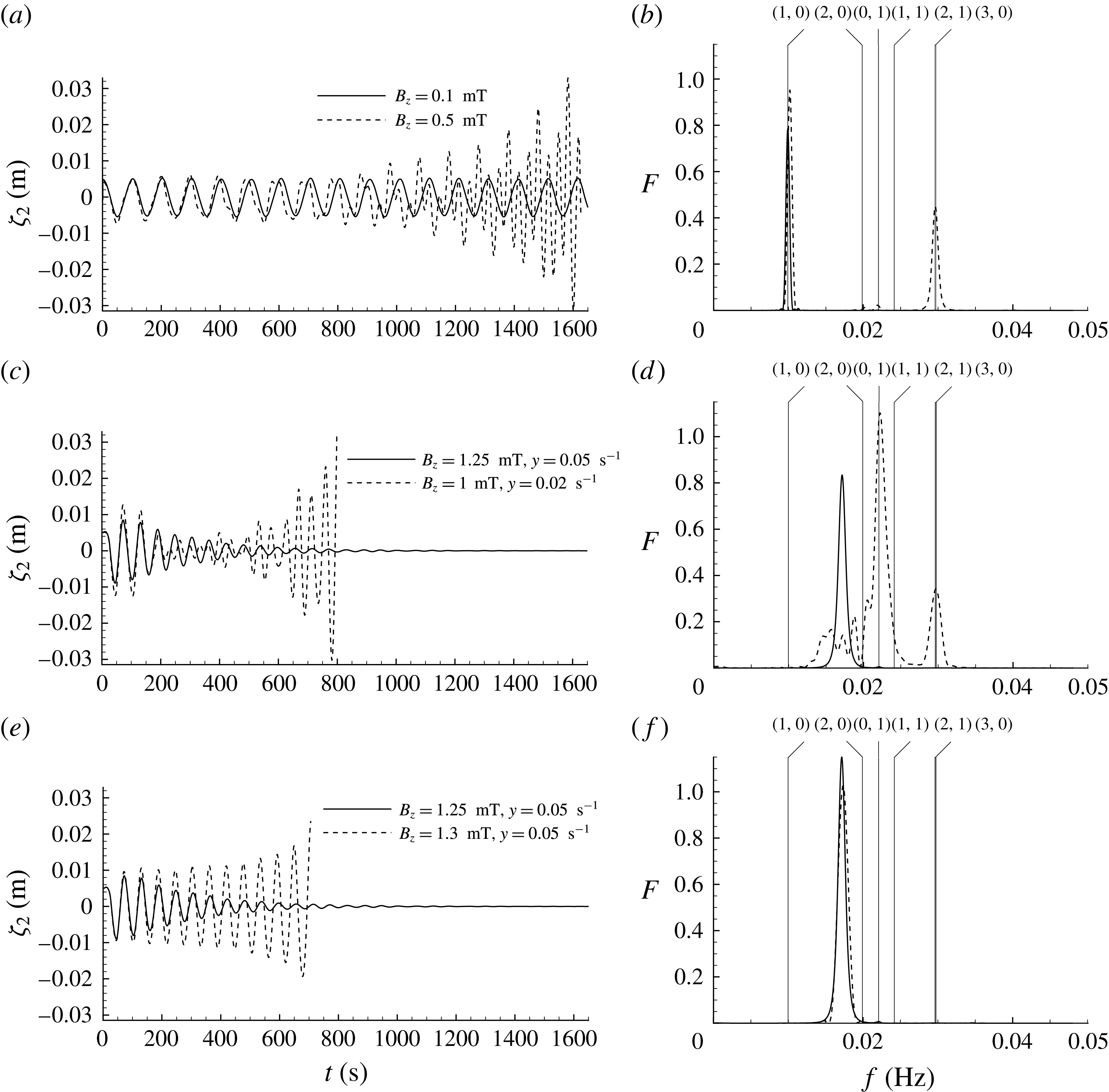
The full 3 layer numerical solution demonstrates that, independently of the initial perturbation type, the instability of the interfacial motion is generated at the frequency that is located between the two closest orthogonal frequencies. For the most important choice of materials (
 $\text{Ca}\Vert \text{Sb}$
,
 $\text{Ca}\Vert \text{Bi}$
,
 $\text{Mg}\Vert \text{Sb}$
) onset of instability is determined by the upper interface (figures 6 and 7). The respective symbols in figure 7 strictly overlap, therefore becoming undistinguishable. This simply means that the decoupled interface approximation is valid.
The computed interface of growing amplitude with friction
 $\unicode[STIX]{x1D6FE}=0.02$
and
 $B_{z}=1$
mT corresponding to figure 8(c,d). The frames at 10 s intervals illustrate the
 $(1,0)+(0,1)$
and
 $(2,1)+(3,0)$
mode interactions: (a)
 $t=635$
s; (b)
 $t=645$
s; (c)
 $t=655$
s; (d)
 $t=665$
s.
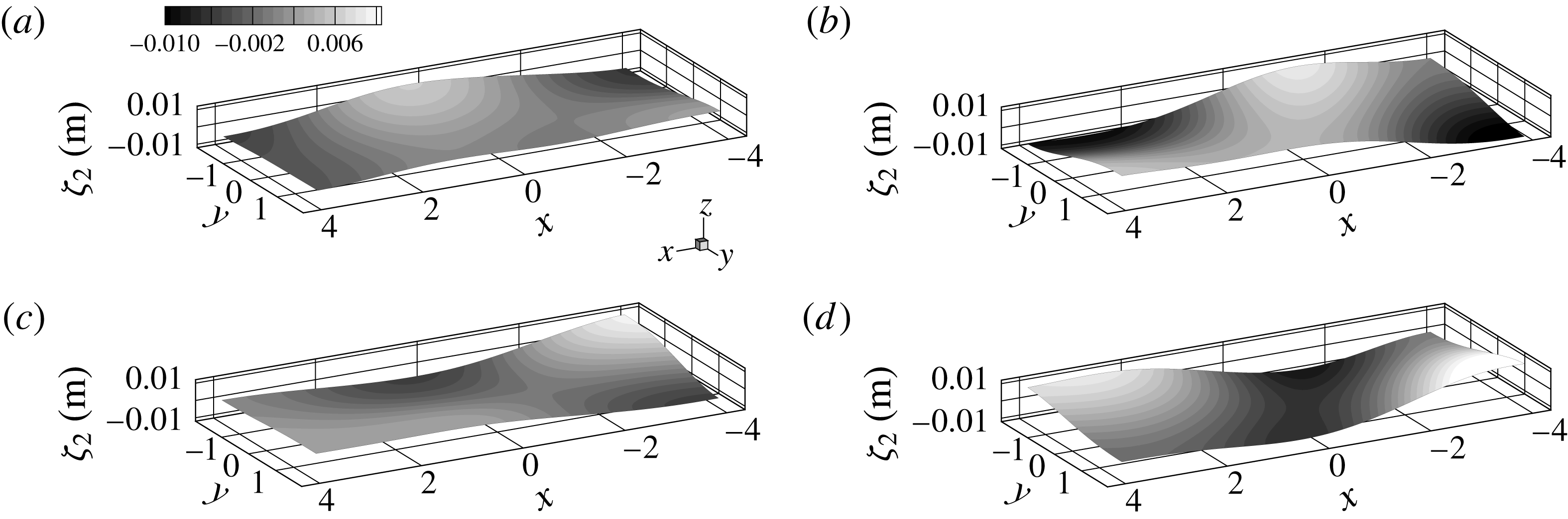
Based on the findings that the top 2 layer model is a good approximation to the LMB stability for the majority of the practically important cases of the material selection, we attempted to compare the previously validated aluminium electrolysis cell numerical models (Bojarevics & Evans Reference Bojarevics and Evans2015) adjusted to the LMB case of the cell geometry given in § 4.2, and for the top metal and electrolyte properties given in table 1. An additional adjustment was required to include numerically the electric current distribution accounting for the bottom metal layer presence. The hydrodynamic model permits inclusion of the wave dissipation effects given by the friction coefficient
 $\unicode[STIX]{x1D6FE}$
as in the linear theory. The initial perturbation of the mode
 $(1,0)$
of amplitude
 $A=0.005$
m and the total electric current
 $I=10^{5}$
A was used in all cases. In the frictionless case
 $\unicode[STIX]{x1D6FE}=0$
at low magnetic field
 $B_{z}=0.1$
mT the sloshing wave is continuously oscillating at the same frequency without signs of significant growth or damping (figure 8
a,b). The MHD interaction of the waves becomes unstable at
 $B_{z}=0.5$
mT after a large number of oscillation cycles as shown in figure 8(a). The Fourier transform of the computed time dependent wave amplitude indicates that the instability sets in due to the dynamic wave transformation resulting in
 $(2,1)+(3,0)$
mode interaction for this particular cell, figure 8(b). The fully coupled linear stability solution results in
 $B^{cr}=0.135$
mT, as shown in figure 7, case 10 for
 $\text{Mg}\Vert \text{Sb}$
. The growth increment in the overcritical regime is extremely low, however increasing with the magnetic field (figure 4). The numerical solution shown in figure 8(a) illustrates the slow growth of the instability. Sneyd & Wang (Reference Sneyd and Wang1994) results for the same
 $(2,1)+(3,0)$
mode interaction in the HHC case predict
 $B^{cr}\approx 0.145$
mT, Bojarevics & Romerio (Reference Bojarevics and Romerio1994) predict
 $B^{cr}\approx 0.135$
mT, whereas Davidson & Lindsay (Reference Davidson and Lindsay1998), based on Gershgorin’s theorem, predict
 $B^{cr}\approx 0.130$
mT. These results show the advantage of using the coupled fluid dynamic stability analysis over the purely mechanical solid plate model developed by Zikanov (Reference Zikanov2015),
 $B^{cr}\approx 11$
mT, and the similar non-inertial result by Sele (Reference Sele1977),
 $B^{cr}\approx 1.8$
mT. The lower stability limit is confirmed independently by the MHD numerical simulations in Weber et al. (Reference Weber, Beckstein, Herreman, Horstmann, Nore, Stefani and Weier2017).
After adding the friction coefficient of the empirical value
 $\unicode[STIX]{x1D6FE}=0.05~\text{s}^{-1}$
, which is close to typical values
 $(0.02{-}0.08)~\text{s}^{-1}$
used for commercial aluminium reduction cells (Zikanov et al.
Reference Zikanov, Thess, Davidson and Ziegler2000; Bojarevics & Evans Reference Bojarevics and Evans2015), the cell becomes unstable at
 $B_{z}=1.3$
mT. The oscillation frequency at the instability onset (see figure 8
f) is well described by the two interacting mode r.m.s. value
 $\unicode[STIX]{x1D6FA}_{(1,0),(0,1)}=0.017$
Hz (4.42). The transition to the instability is rather sensitive to the
 $B_{z}$
value, as can be seen from figure 8(c) showing the damped oscillation for
 $B_{z}=1.25$
mT. For a lower
 $B_{z}$
the damping is dominant, for a higher
 $B_{z}$
the growth rate increases, for example, at
 $B_{z}=1.5$
mT it takes only 97 s for the top interface wave to reach the short circuiting condition at the bottom metal. The typical wave snapshots at the late stage of development are shown in figures 9 and 10. The four frames shown at intervals of approximately a quarter of the period (
 $T_{(2,1)}\approx 33.71$
s) demonstrate a more complex wave rotation pattern than a typical rotating wave along the whole cell perimeter. The instability threshold at
 $\unicode[STIX]{x1D6FE}=0.02~\text{s}^{-1}$
,
 $B_{z}=1$
mT, found from the numerical wave evolution simulation, matches the instability onset according to the analytical criterion (4.48) (see figure 6).
The other transition to instability when the longitudinal mode
 $(1,0)$
interacts with the
 $(0,1)$
transversal mode is reached at a higher friction
 $\unicode[STIX]{x1D6FE}=0.05~\text{s}^{-1}$
and
 $B_{z}=1.3$
mT according to the analytical criterion (4.48) or (4.41), as deduced from figure 6. This is confirmed by the direct numerical wave simulation as shown in figure 8(e). The corresponding ‘rotating’ wave frames are shown in figure 10. The mode
 $(1,0)$
and
 $(0,1)$
interaction occurs at the shifted oscillation frequency
 $\text{Im}(\unicode[STIX]{x1D707})=f$
(4.42) located between the original gravity wave frequencies (figure 8
f).
The computed interface of growing amplitude with
 $\unicode[STIX]{x1D6FE}=0.05$
and
 $B_{z}=1.3$
mT corresponding to figure 8(e,f) for the
 $(1,0)+(0,1)$
mode interaction: (a)
 $t=633$
s; (b)
 $t=640$
s; (c)
 $t=660$
s; (d)
 $t=668$
s.
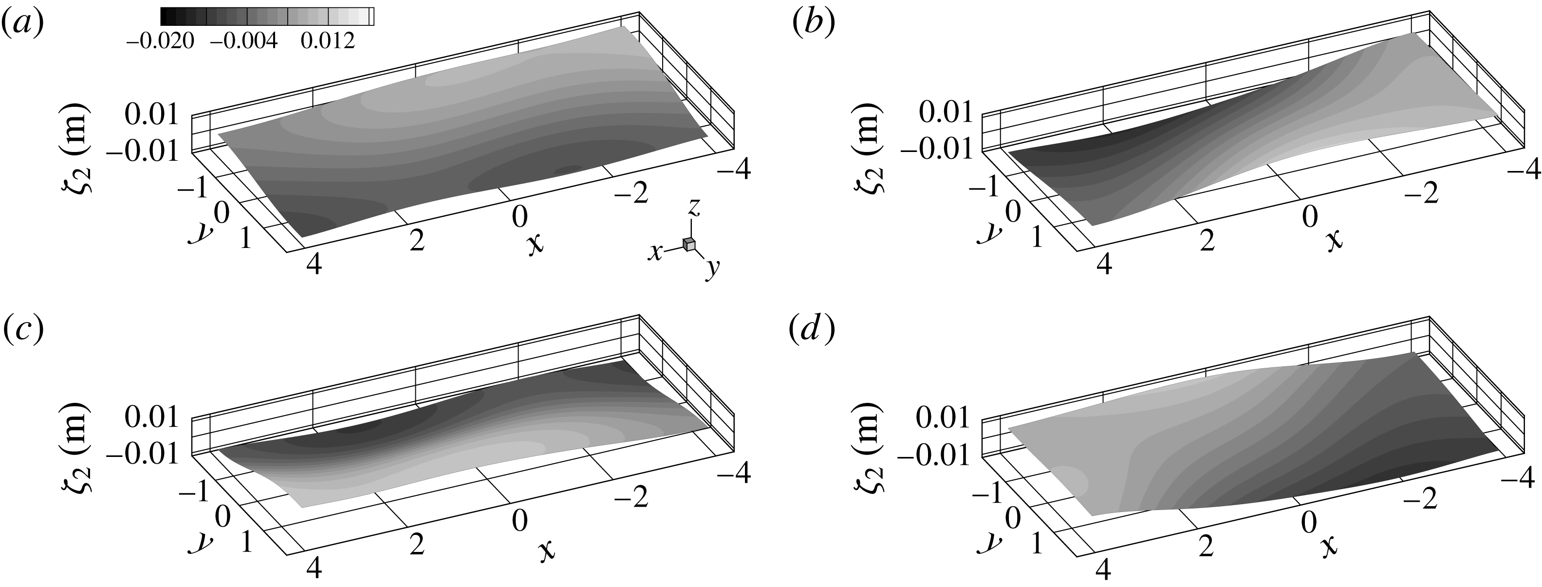
5 Concluding remarks
The presented linear theory derivation focused on the ability to obtain some analytical results for the stability, while intentionally avoiding the more realistic set-up when the electric current supply at the top and bottom collectors is non-uniform. The simplification permitted us to avoid the inclusion of the horizontal velocity circulation effects on the MHD stability. In the general case the curl of electromagnetic force is not identically zero (as shown in § 4.1), leading to the horizontal velocity circulation which can affect the interface deformation. These effects are already analysed numerically in the HHC case (e.g. Bojarevics & Evans Reference Bojarevics and Evans2015) and within the decoupled LMB model Bojarevics & Tucs (Reference Bojarevics and Tucs2017). The full nonlinear interaction in the LMB case remains the subject for a future research.
The method of regular perturbations using the small depth
 $\unicode[STIX]{x1D6FF}$
and the small amplitude
 $\unicode[STIX]{x1D700}$
parameters was applied to reduce the full three-dimensional problem for the electric current distribution and the interface waves in the 3 layer liquid metal battery model.
The linearised equations are solved in the sense of linear stability analysis. For the most important choice of materials in these batteries (high density lower metal and a light metal at the top:
 $\text{Ca}\Vert \text{Sb}$
,
 $\text{Ca}\Vert \text{Bi}$
,
 $\text{Mg}\Vert \text{Sb}$
) the upper interface is the most unstable. The destabilisation mechanism is very similar to the behaviour observed in HHC and confirming with the results in Bojarevics & Tucs (Reference Bojarevics and Tucs2017), Weber et al. (Reference Weber, Beckstein, Herreman, Horstmann, Nore, Stefani and Weier2017) and Zikanov (Reference Zikanov2018). The upper interface waves can be successfully analysed using a simplified two layer approximation, however accounting for the electric current redistribution in the bottom metal.
For batteries with comparable density jumps between the layers (
 $\text{Li}\Vert \text{Te}$
,
 $\text{Na}\Vert \text{Sn}$
,
 $\text{Li}\Vert \text{Bi}$
) both interfaces are significantly deformed, and the behaviour is quite different from the HHC (Horstmann et al.
Reference Horstmann, Weber and Weier2018; Zikanov Reference Zikanov2018). Our results show that the linear stability underestimates the onset of instability compared to the fully coupled 3 layer numerical solution. With the magnetic interaction the asymmetric initial perturbation of the top and bottom layers is always dominant in generating the instability.
The lowest mode
 $(1,0)+(0,1)$
interaction is often the most unstable. For square cells it is always the dominant one leading to instability if even an infinitesimal magnetic field is present (this conclusion holds for shallow systems only
 $\unicode[STIX]{x1D6FF}\ll 1$
) (Bojarevics & Romerio Reference Bojarevics and Romerio1994; Zikanov Reference Zikanov2018). The
 $(1,0)+(0,1)$
interaction can lead to instability in the small size LMBs with
 $L_{x}=L_{y}=0.2$
m.
The dissipation rate is found to be important for practical applications, leading to the faster damping of higher wave modes and the dominance of lower modes. The pure laminar damping (Landau & Lifshitz Reference Landau, Lifshitz, Sykes and Reid1987)
 $\unicode[STIX]{x1D6FE}\approx 0.0007~\text{s}^{-1}$
is insufficient to preclude instability growth for the large size cells (
 $L_{x}=8$
,
 $L_{y}=3.6$
m,
 $h_{2}=0.04$
m) at the typical
 $B^{cr}\approx 0.1$
mT. The instability onset found at
 $B^{cr}\approx 1$
mT and
 $\unicode[STIX]{x1D6FE}=0.02~\text{s}^{-1}$
is more realistic, and it is very close to typical values of
 $\unicode[STIX]{x1D6FE}$
used in HHC (Zikanov et al.
Reference Zikanov, Thess, Davidson and Ziegler2000; Bojarevics & Evans Reference Bojarevics and Evans2015). The derived new analytical criteria including the damping effects for the stability of two mode interaction are compared against the multiple mode numerical solutions, giving a good match for the instability onset. This indicates that the newly developed analytical criteria including the viscous dissipation effects are equally applicable both for the liquid metal batteries and in the case of aluminium electrolysis cells.
Acknowledgement
We acknowledge the idea of the two mode asymptotic interaction to M. Romerio.
Appendix A. Determination of expansion coefficients for electric potential
Taking into account the boundary conditions (3.3), (3.6) and (3.7) for the potential and its normal derivative at the corresponding
 $\unicode[STIX]{x1D700}$
and
 $\unicode[STIX]{x1D6FF}$
equal-order terms, the following coefficient equalities follow at the lower metal interface
 $\overline{z}=\overline{H}_{1}$
:
 $$\begin{eqnarray}\displaystyle & \displaystyle a_{1}=A_{1}=0, & \displaystyle\end{eqnarray}$$
 $$\begin{eqnarray}\displaystyle & \displaystyle c_{1}=C_{1}=0, & \displaystyle\end{eqnarray}$$
 $$\begin{eqnarray}\displaystyle & \displaystyle s_{1}a_{2}=e_{1}, & \displaystyle\end{eqnarray}$$
 $$\begin{eqnarray}\displaystyle & \displaystyle s_{1}A_{2}=E_{1}-\overline{H}_{01}\unicode[STIX]{x2202}_{ii}B_{1}, & \displaystyle\end{eqnarray}$$
 $$\begin{eqnarray}\displaystyle & \displaystyle a_{2}\overline{H}_{01}+b_{2}=b_{1}, & \displaystyle\end{eqnarray}$$
 $$\begin{eqnarray}\displaystyle & \displaystyle A_{2}\overline{H}_{01}+a_{2}\overline{\unicode[STIX]{x1D701}}_{1}+B_{2}=B_{1}. & \displaystyle\end{eqnarray}$$
Similarly at the upper metal interface
 $\overline{z}=\overline{H}_{2}$
:
 $$\begin{eqnarray}\displaystyle & \displaystyle a_{3}=A_{3}=0, & \displaystyle\end{eqnarray}$$
 $$\begin{eqnarray}\displaystyle & \displaystyle c_{3}=C_{3}=0, & \displaystyle\end{eqnarray}$$
 $$\begin{eqnarray}\displaystyle & \displaystyle s_{3}a_{2}=e_{3}, & \displaystyle\end{eqnarray}$$
 $$\begin{eqnarray}\displaystyle & \displaystyle s_{3}A_{2}=E_{3}-\overline{H}_{02}\unicode[STIX]{x2202}_{ii}B_{3}, & \displaystyle\end{eqnarray}$$
 $$\begin{eqnarray}\displaystyle & \displaystyle a_{2}\overline{H}_{02}+b_{2}=b_{3}, & \displaystyle\end{eqnarray}$$
 $$\begin{eqnarray}\displaystyle & \displaystyle A_{2}\overline{H}_{02}+a_{2}\overline{\unicode[STIX]{x1D701}}_{2}+B_{2}=B_{3}. & \displaystyle\end{eqnarray}$$
The supplied current density is given at the bottom and top current collectors,
 $\overline{z}=\overline{H}_{0},\overline{H}_{3}$
:
 $$\begin{eqnarray}\displaystyle & \displaystyle \frac{j}{\unicode[STIX]{x1D6FF}\unicode[STIX]{x1D70E}_{3}}=e_{3}, & \displaystyle\end{eqnarray}$$
 $$\begin{eqnarray}\displaystyle & \displaystyle 0=E_{3}-\overline{H}_{3}\unicode[STIX]{x2202}_{ii}B_{3}, & \displaystyle\end{eqnarray}$$
 $$\begin{eqnarray}\displaystyle & \displaystyle \frac{j}{\unicode[STIX]{x1D6FF}\unicode[STIX]{x1D70E}_{1}}=e_{1}, & \displaystyle\end{eqnarray}$$
 $$\begin{eqnarray}\displaystyle & \displaystyle 0=E_{1}-\overline{H}_{0}\unicode[STIX]{x2202}_{ii}B_{1}. & \displaystyle\end{eqnarray}$$
From (A 1)–(A 16) the unknown coefficients for the unperturbed and perturbed parts can be expressed in terms of
 $b_{1}$
,
 $b_{3}$
and
 $B_{1}$
,
 $B_{3}$
respectively. Combining (A 4), (A 6), (A 10), (A 12), (A 14) and (A 16) leads to the equations for the perturbed potentials:
 $$\begin{eqnarray}\displaystyle & \displaystyle (\overline{H}_{01}-\overline{H}_{0})(\overline{H}_{02}-\overline{H}_{01})\unicode[STIX]{x2202}_{ii}B_{1}+s_{1}(B_{3}-B_{1})=\frac{j}{\unicode[STIX]{x1D6FF}\unicode[STIX]{x1D70E}_{1}}(\overline{\unicode[STIX]{x1D701}}_{2}-\overline{\unicode[STIX]{x1D701}}_{1}), & \displaystyle\end{eqnarray}$$
 $$\begin{eqnarray}\displaystyle & \displaystyle (\overline{H}_{02}-\overline{H}_{01})(\overline{H}_{3}-\overline{H}_{02})\unicode[STIX]{x2202}_{ii}B_{3}-s_{3}(B_{3}-B_{1})=-\frac{j}{\unicode[STIX]{x1D6FF}\unicode[STIX]{x1D70E}_{3}}(\overline{\unicode[STIX]{x1D701}}_{2}-\overline{\unicode[STIX]{x1D701}}_{1}). & \displaystyle\end{eqnarray}$$
After multiplying by
 $\unicode[STIX]{x1D70E}_{1}$
and
 $\unicode[STIX]{x1D70E}_{3}$
respectively, the sum of these equations gives a correlation between the two perturbed potentials:
 $$\begin{eqnarray}\displaystyle -\frac{s_{3}}{s_{1}}(\overline{H}_{01}-\overline{H}_{0})\unicode[STIX]{x2202}_{ii}B_{1}=(\overline{H}_{3}-\overline{H}_{02})\unicode[STIX]{x2202}_{ii}B_{3}, & & \displaystyle\end{eqnarray}$$
which after integration is
 $$\begin{eqnarray}\displaystyle -\frac{s_{3}}{s_{1}}(\overline{H}_{01}-\overline{H}_{0})B_{1}=(\overline{H}_{3}-\overline{H}_{02})B_{3}+C, & & \displaystyle\end{eqnarray}$$
where
 $C$
is a function of
 $x$
and
 $y$
, satisfying
 $\unicode[STIX]{x2202}_{ii}C=0$
. From the boundary conditions (3.8) it follows that on the side walls of the cell
 $\unicode[STIX]{x2202}_{n}C=0$
, meaning that
 $C=\text{const.}=0$
due to the freedom to choose the arbitrary constant in the perturbed potential definition. Physically this means that the perturbed electric current is formed of closed loops within the 3 liquid layers and the potentials are linearly correlated as
 $$\begin{eqnarray}\displaystyle -\frac{\overline{h}_{01}}{s_{1}}B_{1}=\frac{\overline{h}_{03}}{s_{3}}B_{3}. & & \displaystyle\end{eqnarray}$$
Appendix B. Weak formulation
The set of wave equations (4.1), (4.2) with the corresponding boundary conditions (4.3), (4.4) are represented in the weak formulation in the following way:
 $$\begin{eqnarray}\displaystyle & & \displaystyle \int _{\unicode[STIX]{x1D6E4}}(\unicode[STIX]{x2202}_{tt}\unicode[STIX]{x1D701}_{1})q\,\text{d}\unicode[STIX]{x1D70E}+\int _{\unicode[STIX]{x1D6E4}}\unicode[STIX]{x1D6FE}_{1}\unicode[STIX]{x2202}_{t}\unicode[STIX]{x1D701}_{1}q\,\text{d}\unicode[STIX]{x1D70E}-\int _{\unicode[STIX]{x1D6E4}}R_{c,1}\unicode[STIX]{x2202}_{tt}\unicode[STIX]{x1D701}_{2}q\,\text{d}\unicode[STIX]{x1D70E}+\int _{\unicode[STIX]{x1D6E4}}R_{1}\unicode[STIX]{x1D6FC}_{1}^{-1}(\unicode[STIX]{x1D735}\unicode[STIX]{x1D701}_{1},\unicode[STIX]{x1D735}q)\,\text{d}\unicode[STIX]{x1D70E}\nonumber\\ \displaystyle & & \displaystyle \quad =-\int _{\unicode[STIX]{x1D6E4}}\unicode[STIX]{x1D70E}_{1}\unicode[STIX]{x1D6FC}_{1}^{-1}B_{z}^{0}(\unicode[STIX]{x2202}_{y}\unicode[STIX]{x1D6F7}_{1}\unicode[STIX]{x2202}_{x}q-\unicode[STIX]{x2202}_{x}\unicode[STIX]{x1D6F7}_{1}\unicode[STIX]{x2202}_{y}q)\,\text{d}\unicode[STIX]{x1D70E},\end{eqnarray}$$
 $$\begin{eqnarray}\displaystyle & & \displaystyle \int _{\unicode[STIX]{x1D6E4}}(\unicode[STIX]{x2202}_{tt}\unicode[STIX]{x1D701}_{2})q\,\text{d}\unicode[STIX]{x1D70E}+\int _{\unicode[STIX]{x1D6E4}}\unicode[STIX]{x1D6FE}_{2}\unicode[STIX]{x2202}_{t}\unicode[STIX]{x1D701}_{2}q\,\text{d}\unicode[STIX]{x1D70E}-\int _{\unicode[STIX]{x1D6E4}}R_{c,2}\unicode[STIX]{x2202}_{tt}\unicode[STIX]{x1D701}_{1}q\,\text{d}\unicode[STIX]{x1D70E}+\int _{\unicode[STIX]{x1D6E4}}R_{2}\unicode[STIX]{x1D6FC}_{2}^{-1}(\unicode[STIX]{x1D735}\unicode[STIX]{x1D701}_{2},\unicode[STIX]{x1D735}q)\,\text{d}\unicode[STIX]{x1D70E}\nonumber\\ \displaystyle & & \displaystyle \quad =-\int _{\unicode[STIX]{x1D6E4}}\unicode[STIX]{x1D70E}_{3}\unicode[STIX]{x1D6FC}_{2}^{-1}B_{z}^{0}(\unicode[STIX]{x2202}_{x}\unicode[STIX]{x1D6F7}_{3}\unicode[STIX]{x2202}_{y}q-\unicode[STIX]{x2202}_{y}\unicode[STIX]{x1D6F7}_{3}\unicode[STIX]{x2202}_{x}q)\,\text{d}\unicode[STIX]{x1D70E},\end{eqnarray}$$
 $\text{d}\unicode[STIX]{x1D70E}=\text{d}x\,\text{d}y$
and the integration is over
 $\unicode[STIX]{x1D6E4}$
. The set of equations for the electric potentials (3.15), (3.16) with the boundary conditions (3.8) give the following weak form:
 $$\begin{eqnarray}\displaystyle & \displaystyle \int _{\unicode[STIX]{x1D6E4}}h_{1}h_{2}(\unicode[STIX]{x1D735}\unicode[STIX]{x1D6F7}_{1},\unicode[STIX]{x1D735}\unicode[STIX]{x1D713})\,\text{d}\unicode[STIX]{x1D70E}+\int _{\unicode[STIX]{x1D6E4}}\unicode[STIX]{x1D70E}_{e,1}\unicode[STIX]{x1D6F7}_{1}\unicode[STIX]{x1D713}\,\text{d}\unicode[STIX]{x1D70E}=-\frac{j}{\unicode[STIX]{x1D70E}_{1}}\int _{\unicode[STIX]{x1D6E4}}(\unicode[STIX]{x1D701}_{2}-\unicode[STIX]{x1D701}_{1})\unicode[STIX]{x1D713}\,\text{d}\unicode[STIX]{x1D70E}, & \displaystyle\end{eqnarray}$$
 $$\begin{eqnarray}\displaystyle & \displaystyle \int _{\unicode[STIX]{x1D6E4}}h_{2}h_{3}(\unicode[STIX]{x1D735}\unicode[STIX]{x1D6F7}_{3},\unicode[STIX]{x1D735}\unicode[STIX]{x1D713})\,\text{d}\unicode[STIX]{x1D70E}+\int _{\unicode[STIX]{x1D6E4}}\unicode[STIX]{x1D70E}_{e,2}\unicode[STIX]{x1D6F7}_{3}\unicode[STIX]{x1D713}\,\text{d}\unicode[STIX]{x1D70E}=\frac{j}{\unicode[STIX]{x1D70E}_{3}}\int _{\unicode[STIX]{x1D6E4}}(\unicode[STIX]{x1D701}_{2}-\unicode[STIX]{x1D701}_{1})\unicode[STIX]{x1D713}\,\text{d}\unicode[STIX]{x1D70E}. & \displaystyle\end{eqnarray}$$
Appendix C. Numerical time stepping scheme
The set of (4.27) and (4.28) was solved using the second-order-accurate finite difference representation as
 $$\begin{eqnarray}\displaystyle & & \displaystyle \frac{\widehat{\unicode[STIX]{x1D701}}_{1,\boldsymbol{k}}(t_{i+1})-2\widehat{\unicode[STIX]{x1D701}}_{1,\boldsymbol{k}}(t_{i})+\widehat{\unicode[STIX]{x1D701}}_{1,\boldsymbol{k}}(t_{i-1})}{(\unicode[STIX]{x0394}t)^{2}}+\unicode[STIX]{x1D6FE}_{1}\frac{\widehat{\unicode[STIX]{x1D701}}_{1,\boldsymbol{k}}(t_{i+1})-\widehat{\unicode[STIX]{x1D701}}_{1,\boldsymbol{k}}(t_{i-1})}{2\unicode[STIX]{x0394}t}\nonumber\\ \displaystyle & & \displaystyle \quad -\,R_{c,1}\frac{\widehat{\unicode[STIX]{x1D701}}_{2,\boldsymbol{k}}(t_{i+1})-2\widehat{\unicode[STIX]{x1D701}}_{2,\boldsymbol{k}}(t_{i})+\widehat{\unicode[STIX]{x1D701}}_{2,\boldsymbol{k}}(t_{i-1})}{(\unicode[STIX]{x0394}t)^{2}}+\unicode[STIX]{x1D714}_{1,\boldsymbol{k}}^{2}\frac{\widehat{\unicode[STIX]{x1D701}}_{1,\boldsymbol{k}}(t_{i+1})-\widehat{\unicode[STIX]{x1D701}}_{1,\boldsymbol{k}}(t_{i-1})}{2}=\widehat{\unicode[STIX]{x1D6EF}}_{1,\boldsymbol{k}}(t_{i}),\qquad\end{eqnarray}$$
 $$\begin{eqnarray}\displaystyle & & \displaystyle \frac{\widehat{\unicode[STIX]{x1D701}}_{2,\boldsymbol{k}}(t_{i+1})-2\widehat{\unicode[STIX]{x1D701}}_{2,\boldsymbol{k}}(t_{i})+\widehat{\unicode[STIX]{x1D701}}_{2,\boldsymbol{k}}(t_{i-1})}{(\unicode[STIX]{x0394}t)^{2}}+\unicode[STIX]{x1D6FE}_{2}\frac{\widehat{\unicode[STIX]{x1D701}}_{2,\boldsymbol{k}}(t_{i+1})-\widehat{\unicode[STIX]{x1D701}}_{2,\boldsymbol{k}}(t_{i-1})}{2\unicode[STIX]{x0394}t}\nonumber\\ \displaystyle & & \displaystyle \quad -\,R_{c,2}\frac{\widehat{\unicode[STIX]{x1D701}}_{1,\boldsymbol{k}}(t_{i+1})-2\widehat{\unicode[STIX]{x1D701}}_{1,\boldsymbol{k}}(t_{i})+\widehat{\unicode[STIX]{x1D701}}_{1,\boldsymbol{k}}(t_{i-1})}{(\unicode[STIX]{x0394}t)^{2}}+\unicode[STIX]{x1D714}_{2,\boldsymbol{k}}^{2}\frac{\widehat{\unicode[STIX]{x1D701}}_{2,\boldsymbol{k}}(t_{i+1})-\widehat{\unicode[STIX]{x1D701}}_{2,\boldsymbol{k}}(t_{i-1})}{2}=\widehat{\unicode[STIX]{x1D6EF}}_{2,\boldsymbol{k}}(t_{i}),\qquad\end{eqnarray}$$
where
 $\unicode[STIX]{x0394}t$
is the time step. In the numerical examples
 $\unicode[STIX]{x0394}t=0.2$
s was found to be sufficient if comparing to the reduced time step test simulations. The notation
 $\widehat{\unicode[STIX]{x1D6EF}}_{\boldsymbol{k}}$
symbolically represents the combination of the electromagnetic forcing and the nonlinear velocity terms. In the absence of dissipation the numerical solution reproduces the gravity waves corresponding to the analytical solution, see figures 2 and 3.