Introduction
Retinal neurons are spatially arranged in what are commonly termed “retinal mosaics” due to the way that their cell bodies and dendrites tile the retina (Wässle et al., Reference Wässle, Boycott and Illing1981a,Reference Wässle, Peichl and Boycottb). These nonrandom spatial distributions of somas and dendrites are thought to ensure that the visual world is efficiently processed and that nonrandom arrangements may help in the developmental process of wiring up the retina (Galli-Resta, Reference Galli-Resta2002). These retinal mosaics are usually spatially independent, such that there are no spatial relationships between cell bodies of different type. This has been confirmed for a wide range of different neuronal types (Rockhill et al., Reference Rockhill, Euler and Masland2000; Diggle et al., Reference Diggle, Eglen, Troy, Baddeley, Gregori, Mateu, Stoica and Stoyan2006; Eglen & Wong, Reference Eglen and Wong2008). In particular, the spatial positioning of the cell bodies of on- and off-center beta retinal ganglion cells (RGCs) show no spatial relationship to each other, beyond that constrained by cell bodies not overlapping (Eglen et al., Reference Eglen, Diggle and Troy2005).
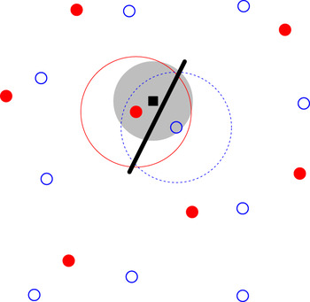
These anatomical studies of RGC arrays have demonstrated little support for the idea of an underlying regular, crystalline, structure. Recently, however, multielectrode recordings have shown that the functional receptive fields of individual types of RGCs tile the retina (Gauthier et al., Reference Gauthier, Field, Sher, Greschner, Shlens, Litke and Chichilnisky2009) in a more regular fashion than either RGC cell bodies or dendritic trees. A recent modeling study (Paik & Ringach, Reference Paik and Ringach2011) proposes that these regular receptive field mosaics play a role in the development of highly structured orientation maps in visual cortex. Given a population of on-center neurons arranged in a noisy hexagonal lattice, and likewise for the off-center neurons, when the two lattices are overlaid, long-range Moiré interference patterns are generated. These hexagonal lattices, representing the RGC receptive field centers, were used as input to a statistical model of wiring from the retina to the cortex (Soodak, Reference Soodak1987; Ringach, Reference Ringach2004, Reference Ringach2007), summarized in Fig. 1. The long-range interference patterns were proposed to drive the generation of regular distributions of orientation pinwheels in visual cortex (Paik & Ringach, Reference Paik and Ringach2011, Reference Paik and Ringach2012). Such regular pinwheel distributions have been suggested to exist in a range of species (Paik & Ringach, Reference Paik and Ringach2011).
Overview of the statistical wiring model. The receptive field midpoints of on- and off-center RGCs (filled red circles and open blue circles, respectively) are arranged in semiregular mosaics. A regular array of cortical neurons (one shown as black square) is overlaid on top of this population. A cortical unit receives input from RGCs whose receptive field centers are within a given range (large filled gray circle) of the cortical neuron, inversely proportional to the lateral distance from the cortical neuron. This cortical unit receives strong input from one on-center and one off-center RGC. These RGCs have Gaussian receptive field profiles (large circles surrounding the two RGCs); the cortical unit thus has an oriented receptive field summarized by the thick black line.

The long-range (>1 mm) Moiré interference patterns generated by hexagonal lattices effectively suggest that there are long-range correlations in the positioning of the receptive fields of RGCs. Here, we use statistical techniques to evaluate how well two competing models can account for the observed spatial distribution of receptive fields. In particular, we compare the hexagonal lattice model with that of a different model where neurons are positioned randomly subject only to exclusion zone constraints; these exclusion zone models have previously been shown to account for a wide range of patterns (Galli-Resta et al., Reference Galli-Resta, Resta, Tan and Reese1997, Reference Galli-Resta, Novelli, Kryger, Jacobs and Reese1999; Cellerino et al., Reference Cellerino, Novelli and Galli-Resta2000). We find that exclusion zone models, but not hexagonal lattice models, can quantitatively account for the observed distributions of receptive field centers. We show that the prediction that retinal mosaics drive the formation of regularly spaced pinwheels in visual cortex critically depends on the long-range correlations generated by the hexagonal lattices. We also estimate the distance over which receptive field centers are correlated from the observed receptive fields. We find no evidence for long-range (>250 μm) correlations in either observed data or exclusion zone models and extensive (>3 mm) correlations in the low noise hexagonal lattice models. We therefore conclude that parasol cell mosaics are too disordered to drive the formation of regular patterns of pinwheels.
Materials and methods
Data sets
Two published data sets of primate parasol cells were analyzed: (1) F07: on- and off-center parasol cells (Fig. 3 of Field & Chichilnisky, Reference Field and Chichilnisky2007) and (2) G09: on- and off-center parasol cells (Fig. 2A and 2B of Gauthier et al., Reference Gauthier, Field, Sher, Greschner, Shlens, Litke and Chichilnisky2009). The receptive field center of each ganglion cell was calculated after thresholding the images. For field G09, the relative positioning of the on- and off-center maps could be determined from their borders. No common border reference was available for field F07 as the receptive fields were recorded separately. One on-center midget cell map was also analyzed (Fig. 2C of Gauthier et al., Reference Gauthier, Field, Sher, Greschner, Shlens, Litke and Chichilnisky2009). This map has a higher density of receptive fields than the parasol cell maps, but several cells were missing from the map. We therefore restricted our analysis of this map to autocorrelation, which is robust to undersampling (Cook, Reference Cook1996). For the analysis of retinal mosaics, each cell is represented by the midpoint of its receptive field.
Simulations of retinal mosaics
We have used the hexagonal lattice model of Paik and Ringach (Reference Paik and Ringach2011). For one mosaic, the lattice separation d is specified in micrometers. We have set d to generate the same number of points as observed in a given area (Table 1). Noise is added to the position of each point in the lattice by drawing samples from the bivariate normal distribution where the standard deviation σ is expressed as a fraction of the lattice separation. When overlaying the on- and off-center mosaics, one map can be rotated by angle θ relative to the other.
Parameter values for each parasol cell mosaic

The number of points and the area of each field were measured from the previous publications (Field & Chichilnisky, Reference Field and Chichilnisky2007; Gauthier et al., Reference Gauthier, Field, Sher, Greschner, Shlens, Litke and Chichilnisky2009). RI denotes the nearest neighbor regularity index (Wässle & Riemann, Reference Wässle and Riemann1978). σ lo and σ hiare the low and high noise levels for the hexagonal lattice simulations, respectively.
The pairwise interaction point process (PIPP) model is simulated as before (Eglen et al., Reference Eglen, Diggle and Troy2005). We assume statistical independence between the on- and off-center mosaics as in principle receptive field midpoints from cells of different type can be the same. [This is to be compared with functional independence previously described for cell body mosaics (Eglen et al., Reference Eglen, Diggle and Troy2005; Diggle et al., Reference Diggle, Eglen, Troy, Baddeley, Gregori, Mateu, Stoica and Stoyan2006).] This means that the on- and off-center mosaics are simulated separately and then overlaid to produce a combined mosaic. To simulate one field, we specify the interaction function h(u) as:
 $$h(u) = 1 - \exp [ - \{ \mu /\varphi \} ^\alpha ],$$
where u is the distance between two points. The two parameters (α and ϕ) control the size of exclusion zone around each point and were chosen by trial-and-error to reproduce the observed spatial patterns. The parameters used for each map are listed in Table 1.
Analysis of retinal mosaics
Established methods were used to quantify the degree of patterning in the observed and simulated mosaics. We also analyze patterns of complete spatial randomness (CSR) as a control for these measures:
1. Voronoi polygons were computed for each point (Fortune, Reference Fortune1987).
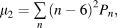
2. Topological disorder, μ 2 (Kram et al., Reference Kram, Mantey and Corbo2010), was quantified using:
 $$\mu _2 = \mathop\sum\limits_n {(n - 6)^2 P_n } ,$$
where Pn is the probability of a Voronoi polygon having n edges. Only Voronoi polygons that did not overlap with the boundary of the sample window were used to estimate Pn. For a perfect hexagonal lattice, all Voronoi polygons will have six edges, and hence, μ 2 = 0. The larger the value of μ 2, the more disordered the pattern. The expectation for CSR is μ 2 = 1.78 (Tanemura, Reference Tanemura2003).
3. Autocorrelograms show the relative displacement between any pair of points within a field (Rodieck, Reference Rodieck1991). The central portion of the autocorrelogram is typically empty, indicating exclusion zones around each point, so that no two points are too close to each other.
4. For each point in a mosaic, the distance to its nearest neighbor was calculated. The G function is the cumulative distribution of these distances (Eglen et al., Reference Eglen, Diggle and Troy2005). The steeper the curve, the more regular the pattern.
5. The L function is the (scaled) expectation of the number of points observed within a given distance of any point (Ripley, Reference Ripley1976; Eglen et al., Reference Eglen, Diggle and Troy2005). For patterns with no spatial structure, we would expect L(t) = t. For regularly spaced patterns, we would expect L(t) < t for small values of t.
Statistical analysis
To evaluate the fit between observed mosaics and simulations, we have calculated Monte Carlo P values using established methods (Diggle, Reference Diggle1986; Eglen et al., Reference Eglen, Diggle and Troy2005). Each model is run, using the same parameters but with different random numbers, 99 times. Each field (both observed and simulated) is then compared against the other 99 fields, and a measure T calculated. The 100 T values are sorted, and the rank of the T measure corresponding to the observed field is divided by 100 to calculate a P value. P values of 0.05 and smaller indicate that the model does not fit the observed data at the 5% significance level. The smallest P value calculated is thus 0.01 with 99 simulations. In addition for the L and G functions, we have drawn the 95% confidence levels from the simulations. Informally, if the measure from the observed mosaics (solid lines in Fig. 2) falls within the confidence intervals (dashed lines), then the model is a good fit to the observed mosaic.
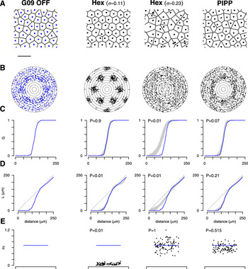
Spatial statistics of the observed off-center receptive field mosaic (Gauthier et al., Reference Gauthier, Field, Sher, Greschner, Shlens, Litke and Chichilnisky2009) (column 1) and three different models (columns 2–4). (A) Central region of the mosaics. Each point denotes one receptive field midpoint and is surrounded by its Voronoi polygon. Scale bar: 250 μm. (B) Autocorrelogram of the points in (A), with annuli drawn 25 μm apart. (C) The G function is the cumulative distribution of nearest neighbor distances. For the models, the gray region shows the 95% confidence interval of distributions from each model, and the solid line reflects the data (also shown in column 1). (D) L functions for data and models, drawn in the same format as for panel (C). The dashed line indicates the expectation for CSR, L(t) = t. (E) Topological disorder μ 2for 99 simulations (black dots) and for the data (horizontal line).

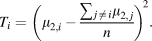
For the topological disorder parameter, μ 2, we plot, as dots, μ 2,i for i = 2…n + 1 simulated mosaics (here, n = 99) along with μ 2,1 of the observed field as a horizontal line. For a good fit between model and data, μ 2,1 should fall within the distribution of simulated values. To compute the P value for μ 2, we calculate Ti for observed and simulated fields:
 $$T_i = \left( {\mu _{2,i} - {{\sum {_{\,j \,\ne \,i} \mu _{2,\,j} } } \over n}} \right)^{\!2}.$$
The T values are then ranked as above to calculate the P value.
Assessing long-range spatial order in retinal mosaics
We used three techniques to estimate the extent of long-range order in retinal mosaics: (1) Kernel density estimates (KDEs), (2) density recovery profiles (DRPs), and (3) assessing structure within each DRP annulus.
Kernel density estimates
Autocorrelograms can be smoothed with kernels; the resulting KDEs can be visualized as images. We have calculated the KDEs of autocorrelograms using the quartic kernel with bandwidth h 0 = 50 μm, with the R function kernel2d (Berman & Diggle, Reference Berman and Diggle1989; Rowlingson & Diggle, Reference Rowlingson and Diggle1993). This method includes edge correction factors to account for the finite extents of the fields being analyzed.
Density recovery profiles
The DRP counts the density of points found in annuli of the autocorrelogram (Rodieck, Reference Rodieck1991). The method includes a compensation factor f (Rodieck, Reference Rodieck1991) to account for the problem that large annuli will often fall outside the sample window and so counts within each annulus will be lower than expected. The compensation factor f is valid for annuli up to half the size of the shortest edge of the rectangular sample window. The experimental fields analyzed here are approximately 1 × 2 mm, so the DRP can be calculated only out to at most 0.5 mm.
As well as calculating the DRP for the experimental fields, we also calculate the DRP for 99 simulations of CSR with matching density to the experimental fields. The DRPs from the CSR fields are used to create 95% confidence intervals of the counts within each annulus to assess what range of values would be expected when there is no spatial structure in the mosaic.
Assessing structure within each DRP annulus
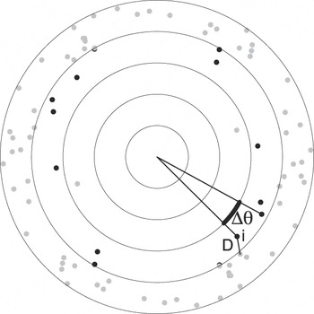
Spatial structure within the autocorrelogram might generate clustering (or repulsion) of points within an annulus of the DRP. By contrast, for points with no spatial structure, we expect points to be randomly distributed within each annulus (except that each pair of points generates two entries in the autocorrelogram opposite each other within the same annulus). To assess this possibility, we defined two new measures for quantifying structure within an annulus (Fig. 8). We take each point within an annulus and measure either the distance to the nearest neighboring point (D) or the angular difference (∆θ) to the next counterclockwise point within the annulus. For each annulus, we plot the cumulative distribution of D or ∆θ for all points within the annulus. (For these calculations, unlike the DRP, there is no compensation factor, but edge effects are expected to be similar when analyzing observed and simulated fields.)
As well as computing the distribution of D and ∆θ for autocorrelograms derived from observed fields, a PIPP simulation, and a hexagonal lattice simulation, we plot the 95% confidence intervals of these measures for autocorrelograms of 99 simulations of CSR. These confidence intervals show the range of values expected when there is no spatial structure in the mosaic. Informally, if the distribution for a field falls within the confidence interval, we suggest that there is no spatial structure of points within that annulus. This can be formalized into an empirical P value using the same formalism as for the G and L functions. P values of 0.05 or less indicate that the distribution of points is nonrandomly distributed at the 5% significance level.
Statistical wiring model
We reimplemented the statistical wiring model for wiring the retina to visual cortex (Fig. 1). All details were taken from previous publications where possible (Ringach, Reference Ringach2004, Reference Ringach2007; Paik & Ringach, Reference Paik and Ringach2011). We simulated a 6 × 6 mm patch of retina, with cellular densities for the on- and off-center RGCs matching field G09. The simulated cortex was 6 × 6 mm with neurons spaced 10 μm apart on a regular square grid. The retina and cortex were aligned to the same size in retinal coordinates so that each RGC had a corresponding preferred location in the cortex. After wiring the retina to the cortex, we shrunk the cortex by a cortical magnification factor of 0.715 because the cortex and retina are of different sizes, as per Paik and Ringach (Reference Paik and Ringach2011). The receptive field of each RGC was modeled as a bivariate Gaussian with standard deviation σ = 60 μm.
Orientation selectivity indexes were computed for each cortical neuron (Ringach, Reference Ringach2007); a neuron was deemed orientation selective if its index exceeded 0.25. The orientation map was then smoothed with a Gaussian window (σ = 140 μm), and the autocorrelation of all oriented cortical units was then calculated and visualized as an image (Paik & Ringach, Reference Paik and Ringach2011). Regularly spaced pinwheels are indicated by repeating peaks in the autocorrelation plot.
Computational environment
All simulations and data analysis were performed in the R programming language, version 2.13.1 (R Development Core Team, 2011), together with extra packages (Rowlingson & Diggle, Reference Rowlingson and Diggle1993; Furrer et al., Reference Furrer, Nychka and Sain2011; Genz & Azzalini, Reference Genz and Azzalini2011). Data files and code are available upon request.
Results
Models of parasol cell mosaics
We first evaluated if the hexagonal lattice model can account for the spatial properties of parasol cell mosaics. We do this independently for on- and off-center mosaics and then combine the two mosaics into one larger population. We have used spatial statistics to quantitatively compare the observed and simulated mosaics. Fig. 2 shows the results for the off-center population from field G09.
Real mosaic
The first column of Fig. 2 shows the analysis of the real mosaic. The points (Fig. 2A) represent the centers of individual off-center parasol cells, overlaid with their Voronoi polygons. The points are regularly arranged, and the autocorrelogram (Fig. 2B) shows a clear exclusion zone of around 100 μm. The G function (Fig. 2C) reports the cumulative distribution of nearest neighbor distances and shows that most nearest neighbors are 100–150 μm apart. Fig. 2D shows the L function, which reports the (scaled) average number of points within a given distance of one neuron. The L function dips below the expectation for a population of points positioned randomly, supporting the notion of an exclusion zone. Finally, in Fig. 2E, we show the topological disorder, μ 2, which measures the variability in the number of Voronoi edges surrounding each point. For the real field in Fig. 2, μ 2= 0.68, indicating a quasiregular population. The absolute values and profiles of these quantitative measures shown in panels C–E are not critical, but instead by calculating the same measures on simulated mosaics, we can then assess how well different models reproduce the observed mosaic.
Hexagonal lattice model
The second column of Fig. 2 shows the results from using the hexagonal lattice model with the same noise level (σ = 0.11) as used previously (Paik & Ringach, Reference Paik and Ringach2011). The autocorrelogram of the simulated points (Fig. 2B, column 1 vs. column 2) shows much more clustering of points than is observed for the real mosaic.
The gray region in Fig. 2C, second column, indicates the 95% confidence interval of the G function, estimated from 99 runs of the hexagonal lattice with the same initial conditions, but using different random numbers in the simulation. We have then overlaid the G function (shown in column 1 of Fig. 2C) from the real mosaic for comparison. The G function for the observed field falls within the confidence interval of the simulations, indicating that the model can reproduce this spatial property of the observed mosaic. This is confirmed with empirical P values (defined in Materials and methods section). P values of 0.05 and smaller indicate that the model does not fit the data at the 5% significance level. Hence, according to the G function, the hexagonal lattice model generates a good fit to the data. This is to be expected, as the nearest neighbor distribution was used to set the noise level (Paik & Ringach, Reference Paik and Ringach2011).
The confidence interval for the L functions from the hexagonal lattice model (Fig. 2D, column 2) shows a different result, however. Beyond about 150 μm, the L function for the hexagonal lattice model begins to oscillate relative to the real data, resulting in a poor fit (P = 0.01). Finally, the values of topological disorder for the hexagonal lattice model are much smaller than the real field, again resulting in a poor fit (P = 0.01). In summary, the hexagonal lattice model generates patterns similar to the observed mosaic according to only one of three quantitative measures.
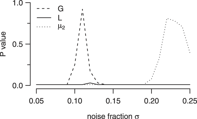
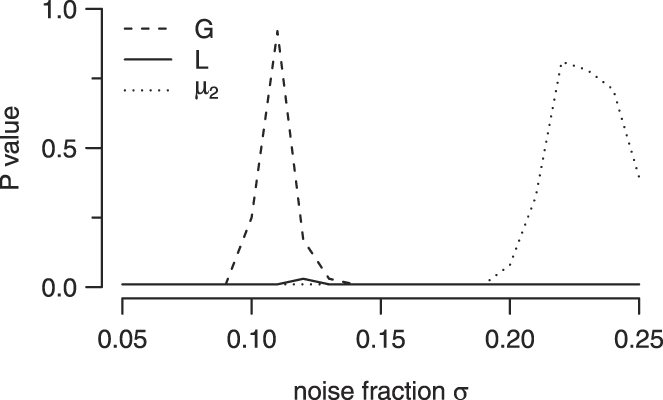
To attempt to improve fits for the hexagonal lattice model, we tried different values of its key parameter, σ, the noise level added to the lattice. As the model was generating patterns that were too regular compared to real mosaics, we tried larger noise levels (shown in Fig. 2, column 3). Increasing the noise level has the predicted effect of making the mosaics less regular, such that an exclusion zone is no longer visible in the autocorrelogram. This relative disorder is reflected in large discrepancies between model and observed mosaic for G and L functions (Fig. 2C and 2D, column 3). However, the increased disorder in the simulated fields generates larger values of μ 2, such that μ 2 for the real field falls within the distribution of simulated μ 2 values. Additional simulations where we systematically varied noise levels (Fig. 3), or imposed a lower bound on the minimal distance allowed, showed a similar trend; we could not find parameters such that there was a good fit between model and data according to all three quantitative measures. We therefore conclude that the hexagonal lattice model, as proposed by Paik and Ringach (Reference Paik and Ringach2011), cannot quantitatively account for the spatial distribution of the receptive fields of parasol cells.
Effect of varying noise fraction in the hexagonal lattice model upon goodness of fit P values between model and the G09 off field. For a given noise level, we ran 99 simulations and evaluated the goodness of fit between model and simulations for three quantitative measures as in Fig. 2. Low noise levels produced good fits for the G function, whereas good fits according to the μ 2 measure required high noise levels. By contrast, no noise level could generate a suitable fit according to the L function.
PIPP model
We therefore turned to a different model of retinal mosaic formation, assuming that cells simply position themselves such that they do not come too close to each other. This idea of an exclusion zone surrounding each neuron was first shown to quantitatively account for the spatial position of cholinergic amacrine neurons in rat (Galli-Resta et al., Reference Galli-Resta, Resta, Tan and Reese1997). It has since replicated a wide range of retinal mosaics (Eglen, Reference Eglen2006). Here, we used the PIPP exclusion zone model, as we have previously shown that it generates mosaics that quantitatively match anatomical RGC mosaics in cat (Eglen et al., Reference Eglen, Diggle and Troy2005). It has also been used in previous models of cortical orientation selectivity (Ringach, Reference Ringach2007). Starting from a random arrangement, points are repositioned randomly subject only to the constraint, determined by an interaction function [h(·), eqn. (1)], that no two points come too close to each other.
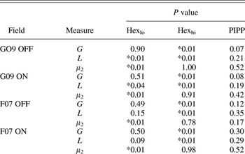
The PIPP model requires two parameters (Table 1) to determine the shape of the exclusion zone around each cell. Fig. 2 (column 4) shows the results of the PIPP model for one field. The autocorrelogram from a simulated mosaic appears similar to that from the real mosaic, which is confirmed by the nonsignificant P values from three quantitative measures (Fig. 2C–2E, column 4; Table 2). Although the real value of μ 2 is slightly higher than the median μ 2 of simulations, it is well within the expected range, as confirmed by the high P value.
Goodness of fit P values for the hexagonal lattice (both low and high noise) and PIPP models for four parasol cell mosaics

P values of 0.05 or less are starred (*) to denote significant difference between model and observed field.
We have performed similar fits for the three other parasol mosaics that were available to us (G09 on-center; F07 on-center; and F07 off-center), and the resulting P values are reported in Table 2. For these three other fields, we found no suitable value of noise level in the hexagonal lattice model could generate a good fit, but that the PIPP model could also account for these fields. We conclude that the PIPP model, but not the noisy hexagonal lattice model, accounts for the spatial properties of parasol cell receptive field mosaics.
Midget cell mosaic
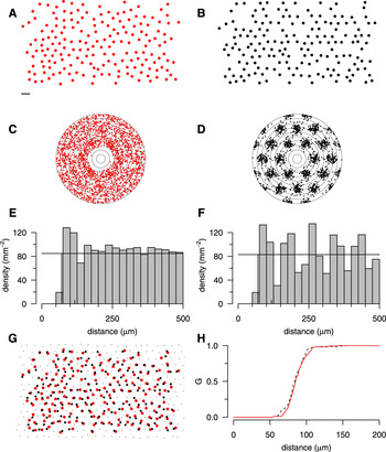
We have also analyzed a denser, but incomplete, mosaic, that of the on-center midget cells (Fig. 4A). Autocorrelation is robust to undersampling of retinal mosaics (Cook, Reference Cook1996); Fig. 2C shows a similar autocorrelogram to that of the parasol mosaics, with a slightly smaller exclusion zone due to the higher density of points. By contrast, the autocorrelogram of an undersampled low noise hexagonal lattice (Fig. 2B and 2D) is much more regular, with strong clustering. The DRPs quantify the difference in the two autocorrelograms. The midget cells (Fig. 2E) have an exclusion zone around 75 μm, and after an increased density around 100 μm, the profile recovers to the mean density. By contrast, after the exclusion zone, the autocorrelogram of the hexagonal lattice shows prominent oscillations. Finally, despite the large differences in the correlograms (Fig. 2Cvs. Fig. 2D), the cumulative nearest neighbor distribution (G) of the two patterns is similar (Fig. 2H). Hence, the G function alone (as used by Paik & Ringach, Reference Paik and Ringach2011) is inappropriate for assessing similarity between real and simulated fields.
Analysis and modeling of on-center midget mosaic. (A) On-center midget mosaic with several missing cells (Gauthier et al., Reference Gauthier, Field, Sher, Greschner, Shlens, Litke and Chichilnisky2009). Scale bar for (A), (B), and (G): 100 μm. (B) Hexagonal lattice mosaic (d = 97 μm, σ = 0.12) with points deleted to match incomplete mosaic in (A); see panel (G) for details. (C, D) Autocorrelogram of mosaics in (A) and (B), with 25 μm annuli. (E, F) DRPs for the mosaics in panel (A) and (B). (G) The simulated mosaic in panel (B) was downsampled from a hexagonal lattice (small and large black dots) covering the extent of observed points (large red dots, taken from panel A). For each observed point, the nearest neighboring simulated point was found (large black dots connected by lines). Only the large black dots were analyzed in panel (B); small black dots were discarded. (H) Despite differences in long-range structure, the cumulative distributions of nearest neighbor distances of observed (solid red line) and simulated (dotted black line) points are similar.

Effect of retinal mosaics upon cortical orientation selectivity
One key difference between the two types of model is that hexagonal lattice models with low noise have an explicit long-range correlation structure, whereas PIPP models do not. In the lattice model, the position of two neurons even several millimeters apart is likely to be highly correlated as they were originally positioned on a lattice with known spacing. By contrast, the PIPP model simply prevents two cells being too close to each other. For the parameters listed in Table 1, this typically means an exclusion zone around each cell of 100–200 μm. In the PIPP model, there is, therefore, no explicit long-range correlation structure imposed upon receptive field positions.
What impact might this presence or absence of long-range correlation of receptive field positions have upon the model of orientation selectivity proposed by Paik and Ringach (Reference Paik and Ringach2011)? The statistical wiring model (Fig. 1) simulates an array of cortical units that receive inputs from topographically appropriate retinal neurons. Each cortical neuron typically receives input from only a few on- and off-center RGCs. The relative position of these retinal inputs directly determines the receptive field of the cortical neuron. Most receptive fields are oriented; cells with an orientation selectivity index over 0.25 were considered orientation selective and further analyzed.
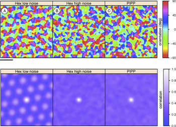
Assuming a hexagonal lattice model for retinal mosaics, the existence of a regular pinwheel organization in orientation tuning maps requires long-range correlational structure, which generates Moiré interference patterns (Paik & Ringach, Reference Paik and Ringach2011). We have verified that hexagonal lattices with low noise can drive the formation of structured orientation columns (Fig. 5A) as shown by highly regular autocorrelational structure. However, if we increase the level of noise in the hexagonal lattice model to more realistic levels, any long-range structure is substantially weakened. Although individual cortical neurons are still orientation selective, the autocorrelation of orientation maps has just a single central peak, indicating no regularity in pinwheel positioning (Fig. 5B). Likewise, when we use mosaics simulated by the PIPP model, as expected, no regular pinwheel structure is observed (Fig. 5C).
Cortical orientation preference maps (top row; scale bar is 1 mm on cortex) and their autocorrelation structure (bottom row; scale bar is 0.81 mm on cortex) generated by statistical wiring model. Hexagonally spaced orientation maps are indicated by repeating peaks in the autocorrelation plot. (A) The hexagonal lattice retinal mosaics with low noise (σ = 0.12) reproduce periodic cortical correlations as reported before (Paik & Ringach, Reference Paik and Ringach2011, Fig. 2C). (B, C) With either high noise (σ = 0.23) hexagonal lattices or PIPP mosaics, periodic cortical correlations are absent.

Hence, we conclude that regular pinwheel structure is critically dependent on the long-range correlations that are present in only the low noise hexagonal lattice, but that these retinal mosaics are unrealistic. As we use more appropriate retinal mosaics, the regular pinwheel structure disappears.
Assessing long-range structure in retinal mosaics
Hexagonal lattices with low noise are inappropriate for capturing local (up to 250 μm) spatial statistics of receptive field mosaics. However, longer-range correlations might be present in the real receptive field mosaics to drive the formation of cortical orientation maps. To assess the extent of long-range structure, we have therefore used three complementary techniques.
Kernel density estimates
Paik and Ringach used KDEs of the autocorrelograms of receptive field centers to support the claim that there are long-range correlations in the real mosaics (e.g., Supplementary Fig. 1 of Paik & Ringach, Reference Paik and Ringach2011). The KDE is a smoothed version of the autocorrelograms presented in Fig. 2B, but typically calculated over longer distances, and estimates the local density of points at any given distance apart.
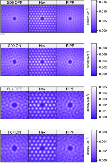
We have calculated the KDE for each autocorrelogram of the four real receptive field mosaics (Fig. 6, left column) along with the KDE of matching simulations from the low noise hexagonal lattice (middle column) and the PIPP model (right column). The KDEs are calculated out to 990 μm from the center (over a square region of edge length 1400 μm). We set the bandwidth of the kernel used for smoothing to 50 μm, as it resulted in a KDE for the G09 off field similar to that shown by Paik and Ringach (Reference Paik and Ringach2011). In each case, the KDE of the real field and the PIPP field is similar, whereas the hexagonal lattice models generate strong peaks and troughs in the KDE. (A feature common to all KDEs is that the density estimates are higher along the X direction than the Y direction; this is simply because fields are twice as wide as they are high.) These KDEs therefore support the notion that hexagonal lattices generate long-range (up to almost 1 mm) correlations, but that these long-range correlations are not observed in either the real data or in the PIPP model. Even though our KDE for off-center field G09 (top left image of Fig. 6) is qualitatively similar to that shown before (supplementary Fig. 1 of Paik & Ringach, Reference Paik and Ringach2011), we have come to a different conclusion because the earlier work did not compare the nature of KDEs under different simulated conditions.
KDEs derived from autocorrelograms of each of the four observed fields and for fields simulated by low noise hexagonal lattice and PIPP model of matching density. Scale bar at top is 200 μm.

Density recovery profiles
The KDEs qualitatively assess the degree of order in autocorrelograms. However, they do not quantify the degree of long-range correlational structure. To do this, we use the DRP (Rodieck, Reference Rodieck1991), probably the most widely used tool for analyzing autocorrelograms of retinal mosaics (Cook, Reference Cook1996; Eglen, Reference Eglen2006). We compare the radial and angular structure of the autocorrelograms from real or simulated mosaics against autocorrelograms of patterns of CSR. This allows us to assess whether the autocorrelogram structure matches that of patterns where there are no correlations at any distance.
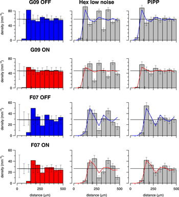
The DRPs for the four observed fields (Fig. 7, left column) all show a similar pattern: an initial exclusion zone out to around 100 μm and then fluctuations around the mean density out to 500 μm, the maximum distance permitted by the correction factors (see Materials and methods section). These fluctuations dampen down by around 200 μm (for field G09) or 350 μm (for field F07, which is of lower density than G09), when the fluctuations are within the 95% confidence intervals of DRPs from CSR simulations. Any radial variation in density of the autocorrelograms of the observed fields is thus not discernible from random by at most 350 μm.
DRPs for observed data, low noise hexagonal lattice, and PIPP model. Left column: The DRP for each observed field; error bars denote 95% confidence intervals of 99 CSR fields of same density as observed field. Solid horizontal line shows the mean density of the observed field. Middle column: Each DRP bar denotes the mean density for 99 simulations of the observed data in left column (shown as solid line); error bars denote 95% confidence intervals of the simulations. The lattice model displays large fluctuations in density at increasing distances, which are absent in the data. Right column: Same as middle column but using the PIPP model. There is good agreement between observed data and PIPP simulations.

The DRPs for the low noise hexagonal lattices (Fig. 7, middle column) show significant differences to the DRPs from the observed fields out to the maximum extent measured. By contrast, the DRPs for the PIPP simulations agree with the DRPs for the observed fields (Fig. 7, right column).
Analysis of autocorrelation structure
The DRP measures radial structure of autocorrelograms but ignores any angular variation in the positioning of points within an annulus. Significant variation of points within an annulus of the DRP might occur if there is strong clustering of points driven by long-range correlations. We have thus devised two new measures (D and ∆θ; defined in Fig. 8 and in Materials and methods section) to quantify any structure within each DRP annulus.
Measuring the structure within an annulus of the autocorrelogram. For each point i within an annulus (here, the third, with its points highlighted in black), D is the distance to the nearest neighboring point; ∆θ is the angular difference to the next counterclockwise point within the annulus.

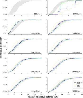
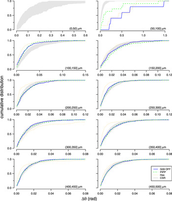
Fig. 9 shows the cumulative distribution of nearest neighbor distances (D) within each annulus of an autocorrelogram for the different patterns. The central circle is empty due to the exclusion zone within the observed and simulated spatial patterns. Up to 200 μm, all three spatial patterns diverge from CSR. This is expected due to the local exclusion zone (Figs. 2 and 7). Beyond 200 μm, the curves for the observed field and the PIPP mosaic fall within the confidence interval for CSR patterns. This indicates that, according to this measure, points within annuli beyond 200 μm for both observed fields and PIPP have no spatial structure. By contrast, the low noise hexagonal lattice model remains outside the CSR envelope. The curve for the low noise hexagonal lattice usually falls to the left of the envelope, indicating more clustering of points than would be expected by chance. This result does not depend on our choice of clustering measure (D); similar results were observed when measuring the distribution of angular differences (∆θ) within each annulus (Fig. 10).
Evaluating structure within each annulus of autocorrelograms using D measure. Each plot shows the cumulative distribution of points within an annulus to their nearest neighbor; each annulus is 50 μm wide, noted in the bottom right of each plot as (lower, upper). The cumulative distribution is shown for observed data (solid blue line: G09 off) and simulations from either PIPP (dashed green line) or low noise hexagonal lattice (dotted orange line). The gray region shows the 95% confidence interval derived from 99 simulations of CSR. See Figs. 11 and 12 for statistical evaluation of the fits between the CSR envelope and the observed and simulated fields.

Evaluating structure within each annulus of autocorrelograms using ∆θ measure. Each plot shows the cumulative distribution of the angular difference of points within an annulus to its counterclockwise neighbor within the annulus. Plots shown in the same format as Fig. 9.

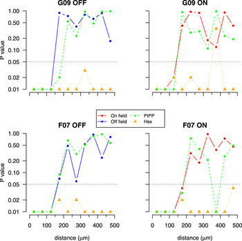
Goodness of fit testing for nearest neighbor distance distributions (D) in autocorrelograms. Each plot calculates the goodness of fit between the autocorrelogram of a field (observed, one PIPP simulation or one low noise hexagonal lattice simulation) and the envelope of 99 CSR simulations as quantified in Fig. 9. An empirical P value is calculated independently for each annulus (50 μm wide) of the autocorrelogram out to a maximum of 500 μm. The y-axis is plotted on a logarithmic scale to emphasize whether the P value is 0.05 (dotted horizontal line) or less. P values of 0.05 or less indicate that the structure of the points within an annulus differs from that expected for random patterns at the 5% significance level.

Goodness of fit testing for angular difference (∆θ) distributions in autocorrelograms. Plots shown in the same format as Fig. 11.

Figs. 11 and 12 quantify the goodness of fit between these distributions and the envelopes expected for autocorrelograms with no spatial structure for all four parasol mosaics. Irrespective of the measure used (D or ∆θ), beyond 200 μm, the structure within the annuli for the experimental data are not significantly different (with only 2 exceptions of 48 annuli) to the autocorrelograms of CSR fields. The P value curves for the PIPP model show a similar trend to the observed fields. By contrast, the P values for the low noise hexagonal lattice are almost always less than 0.05 beyond 200 μm, indicating that the hexagonal lattice model has more structure than that observed.
Taking together the analysis of counts within each DRP annulus (Fig. 7) and the analysis of structure within each annulus of autocorrelograms (Figs. 11 and 12), our estimate of the extent of spatial correlations within the observed fields is 200–350 μm.
Analysis of large simulated mosaics
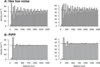
The limited sample size of the observed fields (1 × 2 mm) allows us to calculate the DRP out to at most 0.5 mm (Fig. 7). As larger observed fields are not yet available, we have instead used the simulations of larger fields (6 × 6 mm) to investigate the nature of the DRPs over longer distances (Fig. 13) under different conditions. (These simulated fields were used as input to the cortical model summarized in Fig. 5.)
DRPs for 6 × 6 mm fields simulated to match the spatial statistics of off-center (left column) and on-center (right column) maps from field G09. Each DRP annulus was 50 μm, calculated out to the maximum distance (3 mm) allowed by the compensation factor, but is shown out to only 1.5 mm in (B) as the DRP remained flat beyond 1.5 mm.

For the low noise hexagonal lattice, periodic oscillations around the mean density persist out to 3 mm, the maximal value that we can test (Fig. 13A). For the PIPP model (Fig. 13B), after the exclusion zone, there is a peak (as seen in the G09 off field, Fig. 7, and midget field, Fig. 4E) and modest oscillations that attenuate around 250 μm. Such attenuated oscillations have previously been observed in DRPs of chick photoreceptor mosaics (Fig. 3C of Kram et al., Reference Kram, Mantey and Corbo2010) and cat beta cell mosaics (Zhan & Troy, Reference Zhan and Troy2000) and indicate regularity. After these oscillations, the DRP is flat, indicating no correlations beyond around 250 μm (Fig. 13B).
Correlational distances required for regular pinwheel formation
We estimate that spatial correlations in the experimentally observed fields (and PIPP model) extend to only about 200–350 μm, about 1–2 times d, the spacing of elements in the unjittered hexagonal lattice. This is less than the period of Moiré interference patterns d M = S × d (S = 4–16) predicted for pinwheel formation (Paik & Ringach, Reference Paik and Ringach2011) and much less than the correlational distances of up to 3 mm found in low noise hexagonal lattices (Fig. 13). We conclude that the arrays of receptive field centers of parasol cells do not contain sufficiently long-range correlational structure required by the Paik and Ringach (Reference Paik and Ringach2011) model to seed pinwheel structure.
Discussion
We have analyzed the spatial arrangement of receptive field centers of parasol cells to assess if they contain long-range correlational structure. Such long-range structure in receptive field center positioning might drive the formation of structured orientation pinwheels in visual cortex (Paik & Ringach, Reference Paik and Ringach2011). We find that hexagonal lattices do not adequately account for the spatial statistics observed in all four real parasol cell mosaics that we analyzed, as simulated lattices are too regular. An alternative model (PIPP), where each cell generates a local exclusion zone, provides better fits to the observed data. When more realistic simulated mosaics are input to the statistical wiring model, regularly spaced pinwheels fail to develop, as the mosaics do not contain long-range correlations. Finally, we have estimated the extent to which receptive field center positions are correlated to be only about 200–350 μm. Taken together, we believe that receptive field center mosaics do not contain sufficiently long-range correlation structure to seed pinwheel structure in visual cortex.
Modeling retinal mosaics
The results from Fig. 2 and Table 2 suggest to us that the hexagonal lattice model is too regular to account for receptive field positioning. Previous work modeling cell body mosaics with hexagonal lattices used higher levels of noise (Zhan & Troy, Reference Zhan and Troy2000). As more noise is added to the lattice for modeling receptive field centers, fits to some measures improve but at the expense of worse fits to other measures.
Both hexagonal lattice and PIPP models are phenomenological rather than mechanistic (Eglen, Reference Eglen and Le Novére2012). This is a limitation of both models, but the focus here is on understanding the possible impact of such patterns, rather than how they develop. Despite this, there is a difference in the two models. The PIPP model uses local exclusion zones, typically up to 100–150 μm; no global order is imposed. Molecules (Kay et al., Reference Kay, Chu and Sanes2012) and mechanisms have been proposed to underlie such exclusion zones, including cell death and lateral migration of developing cell bodies (Reese & Galli-Resta, Reference Reese and Galli-Resta2002). By contrast, hexagonal lattice models generate long-range correlations because there is a global pattern imposed on cells within an array. There is no evidence, to our knowledge, for such global prepatterning of retinal mosaics.
We have focused in this paper on the analysis of parasol cell mosaics, as this is the population of primate RGCs for which there is most complete spatial information. We suggest however that midget cells have similar short-range organization, based on analysis of an undersampled mosaic (Fig. 4). Together, both parasol and midget cells account for the majority of RGCs that project to the lateral geniculate nucleus (Perry et al., Reference Perry, Oehler and Cowey1984). We would expect the retinal mosaics of the remaining RGCs to follow similar local organizational principles. However, even if they did exhibit any longer-range organization, its effect is likely to be quite small given they would comprise a minority of RGCs.
Orientation maps in different species
Paik and Ringach (Reference Paik and Ringach2011) showed that the spacing between interference patterns is affected by the angle θ, which determines the orientation of one hexagonal lattice to the other. By varying θ, the statistical wiring model can generate maps that look smooth, as in cat, or with little order among neighboring cortical neurons, as in mouse (Fig. 2 of Paik & Ringach, Reference Paik and Ringach2011). The value of θ is not directly measured, nor estimated, from the observed RGC mosaics but is a free parameter of the hexagonal lattice model that can be varied to generate different patterns.
Within the framework of the statistical wiring model, we suggest an alternative mechanism by which orientation maps can vary (following Sirotin & Das, Reference Sirotin and Das2010). Smooth orientation maps can arise in high-density cortical maps (such as cat or primate) because neighboring cortical neurons are likely to receive similar inputs. By contrast, lower density cortical maps (such as mouse) generate more salt-and-pepper style orientation maps because cortical inputs no longer sample similar inputs. When the density of cortical neurons was reduced 100-fold (to simulate that of a mouse cortex), neighboring cortical neurons no longer shared similar orientation preferences (Hore, Reference Hore2011).
Concerns with the statistical wiring model
Here, we have focused on the nature of retinal mosaics used as input to the statistical wiring model. We have used the cortical model to read out any long-range correlational structure in the retinal mosaics. Although we could replicate the finding that hexagonally spaced pinwheels can emerge from a (low noise) hexagonal lattice, as expected, these regular orientation maps do not form in the absence of retinal long-range correlations.
From a developmental perspective, however, we note several concerns with the statistical wiring model. Most critically, it assumes that the problem of wiring RGCs to the topographically appropriate part of cortex has already been solved. The creation of topographically ordered projections involves many developmental processes (Huberman et al., Reference Huberman, Feller and Chapman2008) each of which are likely to add significant levels of noise to the projections from retina to cortex, perturbing the relative spatial arrangement of retinal inputs. The statistical wiring model also does not describe any possible topographic rearrangements caused by the visual mapping passing through the lateral geniculate nucleus. Nor does it take any account of multiple types of RGC (Field & Chichilnisky, Reference Field and Chichilnisky2007) that independently tile visual space and which could drive orientation selectivity. In particular, midget on- and off-center cells (Fig. 4) are certainly arranged into mosaics at a higher density than parasol cells (Dacey & Petersen, Reference Dacey and Petersen1992; Dacey, Reference Dacey1993). Assuming that the Paik and Ringach model was correct, parasol and midget cells would independently generate patterns on two different spatial scales due to the Moiré interference from the parasol and midget mosaics. This has not been observed. Understanding the development and mechanisms of orientation tuning in visual cortex has a long history, and given other mechanisms that have been proposed (Swindale, Reference Swindale1996), we find the statistical wiring hypothesis unlikely to be a dominant mechanism.
Aside from concerns with the statistical wiring model itself, there are other concerns surrounding the structure of orientation maps. Paik and Ringach (Reference Paik and Ringach2011) present evidence that orientation pinwheels in four different species are hexagonally arranged. Preliminary analysis (Keil et al., 2012)Footnote 1 suggests that the method used by Paik and Ringach to detect hexagonal structure is fairly insensitive, as the method also predicts hexagonality in control maps with no hexagonal structure (Schnabel et al., Reference Schnabel, Kaschube, Löwel and Wolf2007). Alternative methods devised by Keil et al. show that the degree of hexagonal structure found in cortical orientation maps is indistinguishable from these control maps. Hence, not only is there little long-range order in retinal mosaics, cortical orientation maps are unlikely to be hexagonally arranged.
More experimental data are required to examine if there is long-range spatial order in retinal mosaics. We anticipate that larger-scale multielectrode arrays will soon record the receptive field layout of larger populations of neurons (Berdondini et al., Reference Berdondini, Imfeld, Maccione, Tedesco, Neukom, Koudelka-Hep and Martinoia2009). Further technological developments might also allow us to compare the relative organization of physiological and anatomical retinal mosaics. However, using quantitative spatial analysis and computational modeling, we predict that spatial correlations in mosaics are too short ranged to drive regular pinwheel patterns in visual cortex.
Acknowledgments
This work was supported by an EPSRC studentship to V.R.A.H. and a Wellcome Trust program grant (083205/B/07/Z) to S.J.E. Thanks to Prof. William Harris, Dr. Johannes Hjorth, Dr. Wolfgang Keil, Dr. Graeme Mitchison, Dr. David Sterratt, and Prof. David Willshaw for comments on this work.