1 Introduction
Surface-tension-driven thin-film flows arise in a wide range of physical applications. For example, they are crucial in understanding the spreading of liquid films (Oron, Davis & Bankoff Reference Oron, Davis and Bankoff1997; Craster & Matar Reference Craster and Matar2009; Zheng et al. Reference Zheng, Fontelos, Shin, Dallaston, Tseluiko, Kalliadasis and Stone2018), drying of paints (Howison et al. Reference Howison, Moriarty, Ockendon, Terrill and Wilson1997), biological processes such as coating of the internal sides of the airways (Halpern & Grotberg Reference Halpern and Grotberg1992), contact-lens manufacture (Murphy & Lee Reference Murphy and Lee2017), a vast variety of coating processes in industry (Wilson Reference Wilson1982; Howell, Robinson & Stone Reference Howell, Robinson and Stone2013) including spin coating (Fraysse & Homsy Reference Fraysse and Homsy1994; Wilson, Hunt & Duffy Reference Wilson, Hunt and Duffy2000) and spreading of chemical reaction fronts in liquids (Guzman & Vasquez Reference Guzman and Vasquez2016). While the spreading of a fixed volume of fluid is well studied (see, e.g. Voinov Reference Voinov1976; Hocking Reference Hocking1980, Reference Hocking1983, Reference Hocking1992; Lacey Reference Lacey1982; Cox Reference Cox1986; Ehrhard & Davis Reference Ehrhard and Davis1991; King & Bowen Reference King and Bowen2001; Bonn et al. Reference Bonn, Eggers, Indekeu, Meunier and Rolley2009; Savva & Kalliadasis Reference Savva and Kalliadasis2009, Reference Savva and Kalliadasis2013; Howell Reference Howell2010; Ajaev Reference Ajaev2012), the analysis of thin-film flows with sources and sinks is much less common. These flows arise in numerous interesting applications, such as oozing of lava from a volcanic crater (Schwartz & Michaelides Reference Schwartz and Michaelides1988), spreading of films on a porous bed such as textile fabric (Davis & Hocking Reference Davis and Hocking1999, Reference Davis and Hocking2000; Mason & Momoniat Reference Mason and Momoniat2004; Thompson, Tseluiko & Papageorgiou Reference Thompson, Tseluiko and Papageorgiou2015) and droplet spreading with evaporation (Anderson & Davis Reference Anderson and Davis1995; Oliver et al. Reference Oliver, Whiteley, Saxton, Vella, Zubkov and King2015; Saxton et al. Reference Saxton, Whiteley, Vella and Oliver2016). Our interest in thin-film flows with injection is motivated by studying the operation of a purification device that removes gaseous chemicals from an airstream by converting them to liquid through a surface reaction in part of the device. Such injection-spreading problems have been studied in the case when gravity is the driving force for thin-film source flow on an inclined plate (Smith Reference Smith1973; Huppert Reference Huppert1982; Schwartz & Michaelides Reference Schwartz and Michaelides1988; Lister Reference Lister1992), and numerical and similarity solutions have been obtained for the resulting film thickness profile. In particular, Huppert (Reference Huppert1982) also considers the case of a time-dependent source. Duffy & Moffatt (Reference Duffy and Moffatt1997) study a three-dimensional gravity-driven source flow down an almost vertical plane with surface-tension effects included in the steady-flow regime. They find power-law dependencies on the distance down the plane for the width and the height of the resulting film. Further analysis of gravity-driven rivulet flow of Newtonian and power-law fluids down an inclined plane is given in Yatim, Wilson & Duffy (Reference Yatim, Wilson and Duffy2010), whereas shear-stress-driven flow is considered in Yatim, Duffy & Wilson (Reference Yatim, Duffy and Wilson2012). Corresponding travelling-wave similarity solutions are found in Yatim, Duffy & Wilson (Reference Yatim, Duffy and Wilson2013). Momoniat, Ravindran & Roy (Reference Momoniat, Ravindran and Roy2010) consider a similar problem but for radially symmetric spreading with an annular injection slot and investigate the flow behaviour numerically. In Mason & Momoniat (Reference Mason and Momoniat2004) and Momoniat & Mason (Reference Momoniat and Mason2007), symmetry methods from Lie algebras are used to study thin-film flow with injection/suction acting over a porous bed. The related problem of the flow of a viscous film with injection on an inclined porous plane is studied by Thompson et al. (Reference Thompson, Tseluiko and Papageorgiou2015). Here, both surface tension and gravity are included, but the spatial variations of the source term are assumed to be periodic and have zero mean, so that steady-state solutions can be analysed. In addition, the linear stability of these steady states is considered, which reveals that suction and blowing can either increase or decrease the critical Reynolds number for linear stability of these steady states. A different problem is studied in Hocking et al. (Reference Hocking, Sweatman, Fitt and Breward2011), where the blowing is present due to an air jet directed towards a thin film of steel, with the goal of facilitating the coating process. Similar air-jet blowing has been studied in Chilukuri, Aeling & Middleman (Reference Chilukuri, Aeling and Middleman1984) and McKinley, Wilson & Duffy (Reference McKinley, Wilson and Duffy1999), for example. Problems involving thin-film flow with injection of liquid are also studied in the context of elasticity. A concise treatment of the problem of an elastic sheet over a continuously injected viscous fluid is presented in Lister, Peng & Neufeld (Reference Lister, Peng and Neufeld2013). Here, the process under consideration is the peeling of the sheet by bending and pulling at the front facilitated by the injected liquid, and they derive specific propagation laws (governed by the effect of elasticity of the covering membrane) with power-law dependence on time. They also assume the viscous film is situated over a thin pre-wetted layer. A similar problem is considered in Zheng, Griffiths & Stone (Reference Zheng, Griffiths and Stone2015), where buoyancy-driven spreading of a thin film over a membrane with constant injection of liquid is studied. Neglecting the effect of surface tension, they obtain similarity solutions for the position of the liquid front for late time.
A comprehensive review of thin-film equations and spreading is given in Myers (Reference Myers1998), where various thin-film equations are derived. There is a well-known stress singularity at the moving contact line, which is often resolved by assuming that there is precursor layer that pre-wets the substrate and removes the singularity. Such precursor layers are also observed in many physical systems (Bonn et al. Reference Bonn, Eggers, Indekeu, Meunier and Rolley2009; Ajaev Reference Ajaev2012). A comparison between different regularizations (in particular, slip and precursor regularizations) is presented in Savva & Kalliadasis (Reference Savva and Kalliadasis2011) and Sibley et al. (Reference Sibley, Nold, Savva and Kalliadasis2015). The authors conclude that, for certain parameter regimes, the regularizations studied lead to equivalent droplet-spreading behaviours. Asymptotic results for the depth and extent of a steady thin-film flow down an inclined plane that is pre-wetted with a thin precursor layer are given in Benilov et al. (Reference Benilov, Chapman, McLeod, Ockendon and Zubkov2010). In our work, we will be guided by the results obtained in King & Bowen (Reference King and Bowen2001), in which they analyse a general mass-preserving surface-tension-dominated lubrication equation with a very thin precursor layer. However, their results only hold for the spreading of a fixed volume of fluid and do not account for injection of liquid. Lacey (Reference Lacey1982) takes a different approach by assuming a slip regularization, and derives asymptotic results for the spreading of a viscous droplet due to surface tension for late time. Anderson & Davis (Reference Anderson and Davis1995) consider steady and unsteady spreading of an evaporating droplet on a heated surface. They find a relationship between the contact angle and the rate of evaporation, and use asymptotic analysis in the large-capillary-number regime to determine the shape of the droplet. Oliver et al. (Reference Oliver, Whiteley, Saxton, Vella, Zubkov and King2015) consider the surface-tension-driven spreading of a partially wetting drop, assuming a slip regularization, with mass transfer along the entire free surface of the resulting film and, in particular, at the contact line. This leads to appropriate generalizations of Tanner’s law. Similar results are obtained in Saxton et al. (Reference Saxton, Whiteley, Vella and Oliver2016), where the effect of evaporation on the evolution of the contact-set radius is studied. In Saxton et al. (Reference Saxton, Vella, Whiteley and Oliver2017), vapour transport and kinetic effects are used to regularize the mass-flux singularity at the contact line in an evaporating spreading droplet.
In this paper, we will study the surface-tension-driven flow of liquid from a finite-width injection region over a precursor layer. We will explore the problem in which the precursor thickness tends to zero. Initially, we will consider the situation where the production rate is constant, and, therefore, the possibility of a steady state is ruled out. In § 2, we formulate our model, explain and employ the precursor-layer regularization and then non-dimensionalize. In § 3, we present our asymptotic analysis of the problem for early and late times, and briefly consider the
 $O(1)$
-time problem. We will look for power-law predictions for the film thickness in the centre of the injection region, where it attains its maximum, and for the position of the apparent contact line in these temporal regimes. We will present numerical solutions to the full problem and compare them with the asymptotic predictions in § 4. Finally, in §§ 5 and 6, we will consider generalizations to our problem, in which we take more general time- and thickness-dependent source functions, respectively. Further, for power-law-in-time injection, we will suggest a way of predicting the power-law exponent by examining the film thickness profile and the position of the apparent contact line. We draw conclusions and discuss future work in § 7.
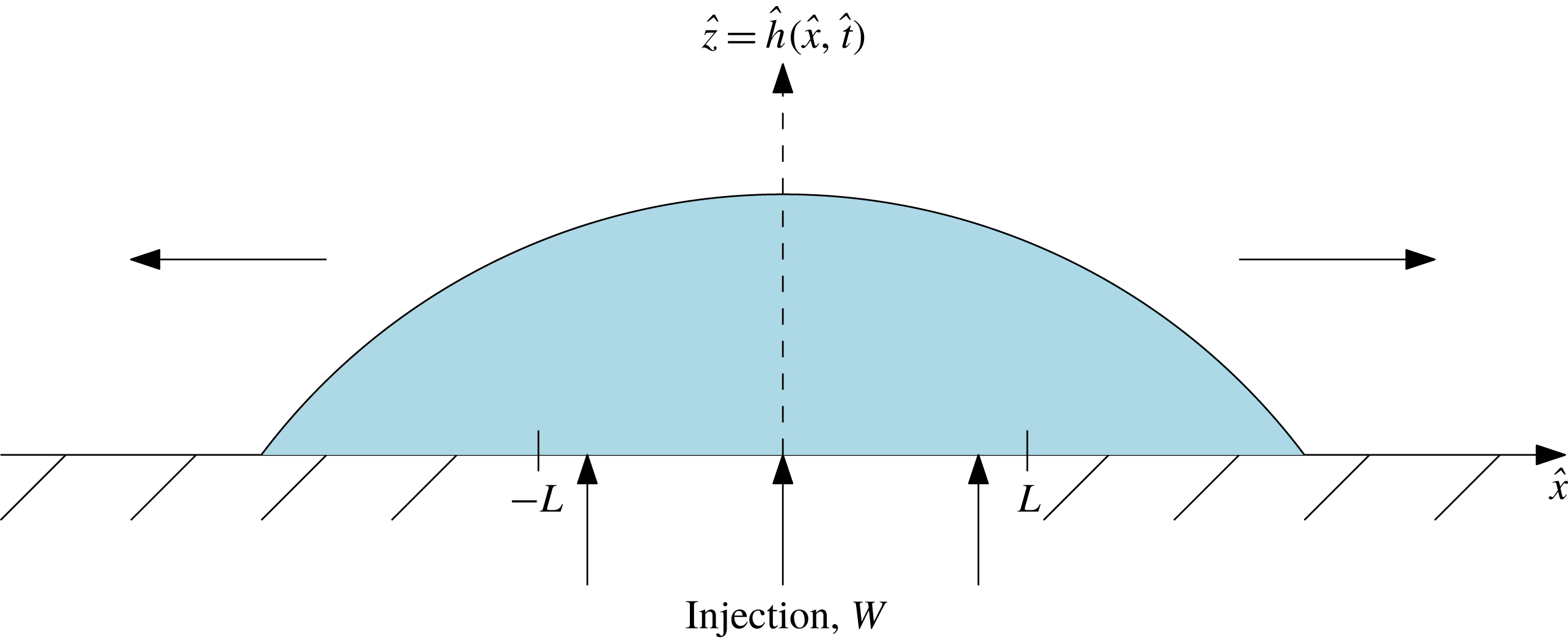
Schematic diagram of the thin-film flow problem with injection in the region
 $-L<\hat{x}<L$
.

2 Mathematical model
2.1 Formulation of the dimensional problem
We consider an infinite one-dimensional substrate, on which viscous liquid is injected uniformly through the surface in the region
 $|\hat{x}|\leqslant L$
at a constant speed
 $W$
. We let
 $\hat{x}$
measure the distance along the substrate and
 $\hat{z}$
measure the distance perpendicular to the substrate, and we show a schematic of the geometry under consideration in figure 1. We expect the reduced Reynolds number to be very small for flows of practical interest in purification devices, and so, we ignore the effect of inertia. Further, assuming that gravity can also be neglected, the flow is surface-tension driven and governed by Stokes’ equations
 $$\begin{eqnarray}\displaystyle & -\unicode[STIX]{x1D735}\hat{p}+\unicode[STIX]{x1D707}\unicode[STIX]{x1D6FB}^{2}\hat{\boldsymbol{u}}=0, & \displaystyle\end{eqnarray}$$
 $$\begin{eqnarray}\displaystyle & \unicode[STIX]{x1D735}\boldsymbol{\cdot }\hat{\boldsymbol{u}}=0, & \displaystyle\end{eqnarray}$$
where
 $\hat{\boldsymbol{u}}=(\hat{u} ,{\hat{w}})$
is the fluid velocity,
 $\hat{p}$
is the pressure and
 $\unicode[STIX]{x1D707}$
is the viscosity of the liquid. We have the following no-slip, kinematic and stress boundary conditions,
 $$\begin{eqnarray}\displaystyle & \hat{u} =0\quad \text{on }\hat{z}=0, & \displaystyle\end{eqnarray}$$
 $$\begin{eqnarray}\displaystyle & {\hat{w}}=W\unicode[STIX]{x1D6E9}(L-|\hat{x}|)\quad \text{on }\hat{z}=0, & \displaystyle\end{eqnarray}$$
 $$\begin{eqnarray}\displaystyle & \displaystyle {\hat{w}}={\displaystyle \frac{\unicode[STIX]{x2202}{\hat{h}}}{\unicode[STIX]{x2202}\hat{t}}}+\hat{u} {\displaystyle \frac{\unicode[STIX]{x2202}{\hat{h}}}{\unicode[STIX]{x2202}\hat{x}}}\quad \text{on }\hat{z}={\hat{h}}(\hat{x},\hat{t}), & \displaystyle\end{eqnarray}$$
 $$\begin{eqnarray}\displaystyle & \displaystyle \hat{\boldsymbol{n}}\boldsymbol{\cdot }\hat{\unicode[STIX]{x1D64F}}\boldsymbol{\cdot }\hat{\boldsymbol{n}}=\unicode[STIX]{x1D6FE}(-\unicode[STIX]{x1D735}\boldsymbol{\cdot }\hat{\boldsymbol{n}})=\unicode[STIX]{x1D6FE}{\displaystyle \frac{\unicode[STIX]{x2202}^{2}{\hat{h}}}{\unicode[STIX]{x2202}\hat{x}^{2}}}\left(1+\left({\displaystyle \frac{\unicode[STIX]{x2202}{\hat{h}}}{\unicode[STIX]{x2202}\hat{x}}}\right)^{2}\right)^{-3/2}\quad \text{on }\hat{z}={\hat{h}}(\hat{x},\hat{t}), & \displaystyle\end{eqnarray}$$
 $$\begin{eqnarray}\displaystyle & \hat{\boldsymbol{n}}\boldsymbol{\cdot }\hat{\unicode[STIX]{x1D64F}}\boldsymbol{\cdot }\hat{\boldsymbol{t}}=0\quad \text{on }\hat{z}={\hat{h}}(\hat{x},\hat{t}), & \displaystyle\end{eqnarray}$$
where
 $\unicode[STIX]{x1D6E9}(\hat{x})$
is the Heaviside step function,
 $\hat{\boldsymbol{t}}$
and
 $\hat{\boldsymbol{n}}$
are the unit tangent and outward-pointing normal vectors to the free surface
 $\hat{z}={\hat{h}}(\hat{x},\hat{t})$
, defined by
 $$\begin{eqnarray}\hat{\boldsymbol{t}}=\left(1+\left({\displaystyle \frac{\unicode[STIX]{x2202}{\hat{h}}}{\unicode[STIX]{x2202}\hat{x}}}\right)^{2}\right)^{-1/2}\left(1,{\displaystyle \frac{\unicode[STIX]{x2202}{\hat{h}}}{\unicode[STIX]{x2202}\hat{x}}}\right),\quad \hat{\boldsymbol{n}}=\left(1+\left({\displaystyle \frac{\unicode[STIX]{x2202}{\hat{h}}}{\unicode[STIX]{x2202}\hat{x}}}\right)^{2}\right)^{-1/2}\left(-{\displaystyle \frac{\unicode[STIX]{x2202}{\hat{h}}}{\unicode[STIX]{x2202}\hat{x}}},1\right),\end{eqnarray}$$
 $\unicode[STIX]{x1D6FE}$
is the (constant) surface tension and
 $\hat{\unicode[STIX]{x1D64F}}$
is the stress tensor, defined by
 $$\begin{eqnarray}\hat{\unicode[STIX]{x1D64F}}=\left(\begin{array}{@{}cc@{}}-\hat{p}+2\unicode[STIX]{x1D707}{\displaystyle \frac{\unicode[STIX]{x2202}\hat{u} }{\unicode[STIX]{x2202}\hat{x}}} & \unicode[STIX]{x1D707}\left({\displaystyle \frac{\unicode[STIX]{x2202}\hat{u} }{\unicode[STIX]{x2202}\hat{z}}}+{\displaystyle \frac{\unicode[STIX]{x2202}{\hat{w}}}{\unicode[STIX]{x2202}\hat{x}}}\right)\\ \unicode[STIX]{x1D707}\left({\displaystyle \frac{\unicode[STIX]{x2202}\hat{u} }{\unicode[STIX]{x2202}\hat{z}}}+{\displaystyle \frac{\unicode[STIX]{x2202}{\hat{w}}}{\unicode[STIX]{x2202}\hat{x}}}\right) & -\hat{p}+2\unicode[STIX]{x1D707}{\displaystyle \frac{\unicode[STIX]{x2202}{\hat{w}}}{\unicode[STIX]{x2202}\hat{z}}}\end{array}\right),\end{eqnarray}$$
and evaluated on the free surface.
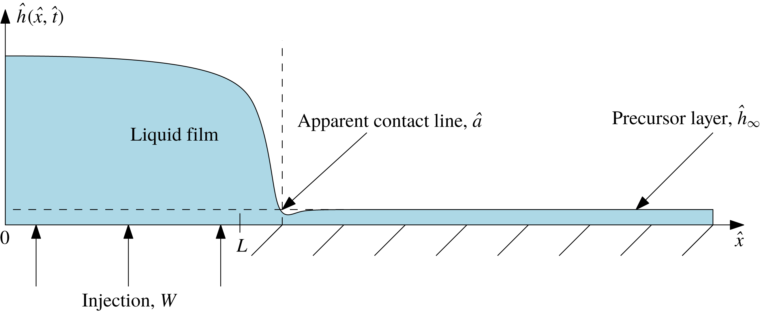
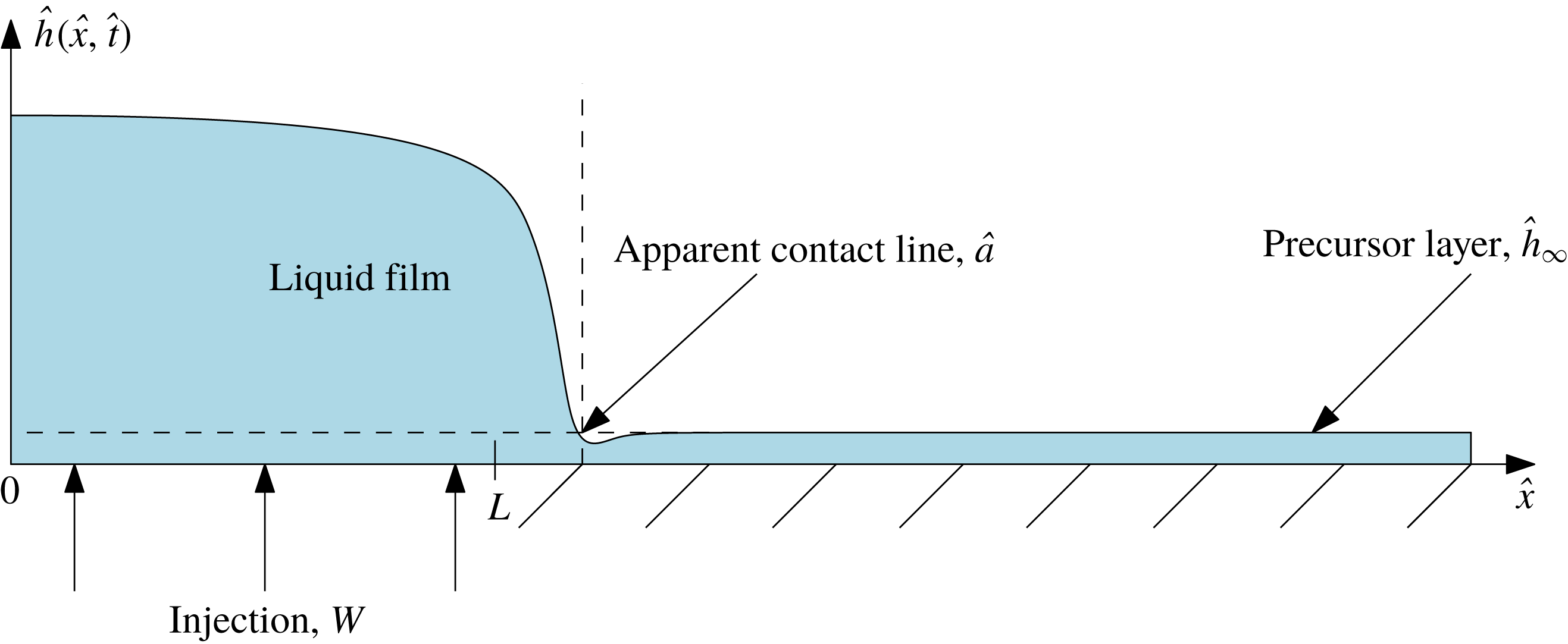
A schematic diagram of the thin-film problem on half-space with injection and a precursor layer of thickness
 ${\hat{h}}_{\infty }$
.
At the moving front,
 $\hat{x}=\hat{a}(\hat{t})$
, say, we could impose zero-thickness and no-flux conditions along with a slip law along the whole of the substrate. For late time, as in the non-injection case we expect a quasi-static profile for the film thickness, where the relationship between the dynamic contact angle,
 $\unicode[STIX]{x1D703}_{d}$
, and the speed of the contact line,
 $\dot{\hat{a}}$
(where a dot
 $(\dot{\,})$
denotes differentiation with respect to time), is given by a version of Tanner’s law. For small contact angles, this can be written as
 $$\begin{eqnarray}{\displaystyle \frac{\unicode[STIX]{x2202}{\hat{h}}}{\unicode[STIX]{x2202}\hat{x}}}=\hat{k}\dot{\hat{a}}^{1/3},\end{eqnarray}$$
for some constant of proportionality
 $\hat{k}$
, depending on the system under consideration (Tanner Reference Tanner1979; Myers Reference Myers1998).
However, instead we choose to regularize the problem using a precursor-film regularization. In this regularization, we assume that the whole substrate is initially covered in a thin layer of liquid of thickness
 ${\hat{h}}_{\infty }$
(see figure 2). Thus, we assume that
 $$\begin{eqnarray}{\hat{h}}\rightarrow {\hat{h}}_{\infty }\quad \text{as }\hat{x}\rightarrow \infty ,\end{eqnarray}$$
and
 $$\begin{eqnarray}{\hat{h}}={\hat{h}}_{\infty }\quad \text{at }\hat{t}=0.\end{eqnarray}$$
This regularization is sufficient to close the problem (King & Bowen Reference King and Bowen2001), it resolves the well-known stress singularity that occurs at the moving contact line in film-spreading problems (Huh & Scriven Reference Huh and Scriven1971), and we will find that this recovers a version of Tanner’s law describing the motion of the apparent contact line,
 $\hat{a}$
. The position of the apparent contact line, which lies in a narrow region where the film thickness adjusts to the precursor thickness, is sometimes defined as the point where the curvature of the free surface attains a local maximum (see, for example, Ajaev Reference Ajaev2012; Carlson, Mandre & Mahadevan Reference Carlson, Mandre and Mahadevan2015). However, any point in the narrow transition region can serve as a definition for the contact line. For concreteness, in this analysis, as well as the numerical solutions, we define the position of the contact line to be the smallest value of
 $\hat{x}$
at which
 ${\hat{h}}$
equals the precursor-layer thickness,
 ${\hat{h}}_{\infty }$
(see figure 2).
Our final lateral boundary conditions are to assume symmetry at
 $\hat{x}=0$
, i.e.
 $$\begin{eqnarray}\hat{u} ={\displaystyle \frac{\unicode[STIX]{x2202}\hat{p}}{\unicode[STIX]{x2202}\hat{x}}}={\displaystyle \frac{\unicode[STIX]{x2202}{\hat{h}}}{\unicode[STIX]{x2202}\hat{x}}}={\displaystyle \frac{\unicode[STIX]{x2202}^{3}{\hat{h}}}{\unicode[STIX]{x2202}\hat{x}^{3}}}=0\quad \text{at }\hat{x}=0.\end{eqnarray}$$
From now on, we assume
 $x\geqslant 0$
and will drop the modulus sign on the right-hand side of (2.4).
2.2 Dimensionless model
We non-dimensionalize (2.1)–(2.7) using
 $$\begin{eqnarray}\left.\begin{array}{@{}c@{}}(\hat{x},\hat{a})=L(x,a),\quad (\hat{z},{\hat{h}})=(\unicode[STIX]{x1D707}WL^{4}/\unicode[STIX]{x1D6FE})^{1/4}(z,h),\\ \hat{u} =(\unicode[STIX]{x1D6FE}W^{3}/\unicode[STIX]{x1D707})^{1/4}u,\quad {\hat{w}}=Ww,\quad \hat{t}=(\unicode[STIX]{x1D707}L^{4}/\unicode[STIX]{x1D6FE}W^{3})^{1/4}t,\quad \hat{p}=(\unicode[STIX]{x1D707}W\unicode[STIX]{x1D6FE}^{3}/L^{4})^{1/4}p.\end{array}\right\}\end{eqnarray}$$
We note that we have chosen the intrinsic scale for
 ${\hat{h}}$
that emerges as a result of non-dimensionalizing (2.6) and balancing viscous forces in the normal direction with surface-tension forces. We assume that the aspect ratio in the problem
 $\unicode[STIX]{x1D716}=\left(\unicode[STIX]{x1D707}W/\unicode[STIX]{x1D6FE}\right)^{1/4}\ll 1$
, and expand the dependent variables in asymptotic series in powers of
 $\unicode[STIX]{x1D716}^{2}$
. This gives the following leading-order dimensionless problem
 $$\begin{eqnarray}\displaystyle & \displaystyle -{\displaystyle \frac{\unicode[STIX]{x2202}p}{\unicode[STIX]{x2202}x}}+{\displaystyle \frac{\unicode[STIX]{x2202}^{2}u}{\unicode[STIX]{x2202}z^{2}}}=0, & \displaystyle\end{eqnarray}$$
 $$\begin{eqnarray}\displaystyle & \displaystyle -{\displaystyle \frac{\unicode[STIX]{x2202}p}{\unicode[STIX]{x2202}z}}=0, & \displaystyle\end{eqnarray}$$
 $$\begin{eqnarray}\displaystyle & \displaystyle {\displaystyle \frac{\unicode[STIX]{x2202}u}{\unicode[STIX]{x2202}x}}+{\displaystyle \frac{\unicode[STIX]{x2202}w}{\unicode[STIX]{x2202}z}}=0, & \displaystyle\end{eqnarray}$$
together with
 $$\begin{eqnarray}\displaystyle & u=0\quad \text{on }z=0, & \displaystyle\end{eqnarray}$$
 $$\begin{eqnarray}\displaystyle & w=\unicode[STIX]{x1D6E9}(L-x)\quad \text{on }z=0, & \displaystyle\end{eqnarray}$$
 $$\begin{eqnarray}\displaystyle & \displaystyle w={\displaystyle \frac{\unicode[STIX]{x2202}h}{\unicode[STIX]{x2202}t}}+u{\displaystyle \frac{\unicode[STIX]{x2202}h}{\unicode[STIX]{x2202}x}}\quad \text{on }z=h(x,t), & \displaystyle\end{eqnarray}$$
 $$\begin{eqnarray}\displaystyle & \displaystyle p=-{\displaystyle \frac{\unicode[STIX]{x2202}^{2}h}{\unicode[STIX]{x2202}x^{2}}}\quad \text{on }z=h(x,t), & \displaystyle\end{eqnarray}$$
 $$\begin{eqnarray}\displaystyle & \displaystyle {\displaystyle \frac{\unicode[STIX]{x2202}u}{\unicode[STIX]{x2202}z}}=0\quad \text{on }z=h(x,t). & \displaystyle\end{eqnarray}$$
Integrating (2.17), and using (2.15)–(2.16) together with (2.18)–(2.22), we find that
 $h$
satisfies the lubrication equation
 $$\begin{eqnarray}{\displaystyle \frac{\unicode[STIX]{x2202}h}{\unicode[STIX]{x2202}t}}+\frac{1}{3}{\displaystyle \frac{\unicode[STIX]{x2202}}{\unicode[STIX]{x2202}x}}\left(h^{3}{\displaystyle \frac{\unicode[STIX]{x2202}^{3}h}{\unicode[STIX]{x2202}x^{3}}}\right)=\unicode[STIX]{x1D6E9}(1-x).\end{eqnarray}$$
The dimensionless boundary and initial conditions become
 $$\begin{eqnarray}\displaystyle & \displaystyle {\displaystyle \frac{\unicode[STIX]{x2202}h}{\unicode[STIX]{x2202}x}}={\displaystyle \frac{\unicode[STIX]{x2202}^{3}h}{\unicode[STIX]{x2202}x^{3}}}=0\quad \text{at }x=0, & \displaystyle\end{eqnarray}$$
 $$\begin{eqnarray}\displaystyle & h\rightarrow \unicode[STIX]{x1D6FF}\quad \text{as }x\rightarrow \infty , & \displaystyle\end{eqnarray}$$
 $$\begin{eqnarray}\displaystyle & h=\unicode[STIX]{x1D6FF}\quad \text{at }t=0, & \displaystyle\end{eqnarray}$$
where
 $\unicode[STIX]{x1D6FF}={\hat{h}}_{\infty }/(\unicode[STIX]{x1D716}L)\ll 1$
is the dimensionless precursor-film thickness and the only remaining parameter in the system. Although we have only three boundary conditions for our fourth-order equation, the precursor-layer regularization (2.25) is enough to ensure a unique solution (Myers Reference Myers1998; King & Bowen Reference King and Bowen2001).
Integrating (2.23) with respect to both
 $x$
and
 $t$
and applying (2.24) and (2.26), we obtain
 $$\begin{eqnarray}\int _{0}^{\infty }(h(x,t)-\unicode[STIX]{x1D6FF})\,\text{d}x=t.\end{eqnarray}$$
Equation (2.27) is an alternative expression for global conservation of mass, but will be convenient to use in the following analysis.
In the next section, we will explore the behaviour of the film thickness for early,
 $O(1)$
, and late time, which will enable us to make substantial analytical progress with the problem.
3 Asymptotic analysis in the limit
 $\unicode[STIX]{x1D6FF}\ll 1$

We begin by considering the asymptotic behaviour in
 $\unicode[STIX]{x1D6FF}$
of (2.23)–(2.27) for early,
 $O(1)$
, and late time, and will later compare the results with the full numerical solution. We will find that (i) it is straightforward to determine the early-time behaviour, (ii) the
 $O(1)$
-time behaviour is identical to the case of zero injection and (iii) the interesting injection-dependent behaviour occurs at late time.
3.1 Early-time behaviour
To examine the early-time behaviour of
 $h$
, we rescale the thickness
 $h$
with the initial thickness,
 $\unicode[STIX]{x1D6FF}$
, and scale time to balance the film growth with the liquid supply, i.e. we set
 $$\begin{eqnarray}h=\unicode[STIX]{x1D6FF}\tilde{h},\quad t=\unicode[STIX]{x1D6FF}\tilde{t}.\end{eqnarray}$$
We pose the asymptotic expansions
 $$\begin{eqnarray}\displaystyle & \tilde{h}(x,\tilde{t})\sim \tilde{h}_{0}(x,\tilde{t})+\unicode[STIX]{x1D6FF}\tilde{h}_{1}(x,\tilde{t})+\cdots \quad \text{as }\unicode[STIX]{x1D6FF}\rightarrow 0, & \displaystyle\end{eqnarray}$$
 $$\begin{eqnarray}\displaystyle & a(\tilde{t})\sim 1+\unicode[STIX]{x1D6FF}a_{1}(\tilde{t})+\cdots \quad \text{as }\unicode[STIX]{x1D6FF}\rightarrow 0, & \displaystyle\end{eqnarray}$$
and assume, following King & Bowen (Reference King and Bowen2001), that on this time scale the apparent contact line moves only an
 $O(\unicode[STIX]{x1D6FF})$
distance from its original location at the end of the injection region. Thus, to leading order we have
 $$\begin{eqnarray}{\displaystyle \frac{\unicode[STIX]{x2202}\tilde{h}_{0}}{\unicode[STIX]{x2202}\tilde{t}}}=\unicode[STIX]{x1D6E9}(1-x),\end{eqnarray}$$
with initial condition
 $$\begin{eqnarray}\tilde{h}_{0}=1\quad \text{at }\tilde{t}=0.\end{eqnarray}$$
The solution, in terms of the original variables, is
 $$\begin{eqnarray}h_{0}(x,t)=\unicode[STIX]{x1D6FF}+t\unicode[STIX]{x1D6E9}(1-x).\end{eqnarray}$$
We immediately note that, since this solution is spatially uniform on either side of
 $x=1$
, the boundary conditions (2.24) are automatically satisfied. The global conservation of mass (2.27) also holds. However, there is a discontinuity in our solution at
 $x=1$
and, to determine the smooth transition between the two solutions given in (3.6), we need to consider a boundary layer near
 $x=1$
. Specifically, we rescale
 $$\begin{eqnarray}x=1+\unicode[STIX]{x1D6FF}\tilde{x}.\end{eqnarray}$$
In this boundary layer, we obtain the following problem
 $$\begin{eqnarray}{\displaystyle \frac{\unicode[STIX]{x2202}\tilde{h}}{\unicode[STIX]{x2202}\tilde{t}}}+\frac{1}{3}{\displaystyle \frac{\unicode[STIX]{x2202}}{\unicode[STIX]{x2202}\tilde{x}}}\left(\tilde{h}^{3}{\displaystyle \frac{\unicode[STIX]{x2202}^{3}\tilde{h}}{\unicode[STIX]{x2202}\tilde{x}^{3}}}\right)=\unicode[STIX]{x1D6E9}(-\tilde{x}),\end{eqnarray}$$
subject to
 $$\begin{eqnarray}\displaystyle & \tilde{h}\rightarrow 1\quad \text{as }\tilde{x}\rightarrow \infty , & \displaystyle\end{eqnarray}$$
 $$\begin{eqnarray}\displaystyle & \tilde{h}\rightarrow 1+\tilde{t}\quad \text{as }\tilde{x}\rightarrow -\infty , & \displaystyle\end{eqnarray}$$
 $$\begin{eqnarray}\displaystyle & \tilde{h}=1\quad \text{at }\tilde{t}=0. & \displaystyle\end{eqnarray}$$
We will solve this boundary-layer problem numerically in § 4.
Before we focus on the behaviour of the thickness of the liquid film
 $h(x,t)$
for late time when we expect
 $O(1)$
movement of the contact line, we look at the
 $O(1)$
-time problem and discuss the behaviour of the apparent contact line.
3.2 The
$O(1)$
-time behaviour

For
 $O(1)$
time, all terms in (2.23) come into play, and analytical progress is difficult. However, we will carefully analyse the motion of the apparent contact line with the purpose of exploiting these results during the late-time analysis. The scalings that we obtain in this section are identical to those used in the no-injection case considered in King & Bowen (Reference King and Bowen2001). They find that the apparent contact line is stationary for
 $O(1)$
time, which is supported by our numerical solutions found in § 4. We will focus on the next-order correction to this leading-order behaviour. Following the work of King & Bowen (Reference King and Bowen2001), we note that the leading-order (in
 $\unicode[STIX]{x1D6FF}$
) solution for
 $h$
in the injection region has the following behaviour as
 $x\rightarrow 1^{-}$
 $$\begin{eqnarray}h_{0}\sim A(t)(1-x)\quad \text{as }x\rightarrow 1^{-},\end{eqnarray}$$
where
 $A(t)>0$
is some function that can, in theory, be determined from solving the leading-order problem
 $$\begin{eqnarray}{\displaystyle \frac{\unicode[STIX]{x2202}h_{0}}{\unicode[STIX]{x2202}t}}+\frac{1}{3}{\displaystyle \frac{\unicode[STIX]{x2202}}{\unicode[STIX]{x2202}x}}\left(h_{0}^{3}{\displaystyle \frac{\unicode[STIX]{x2202}^{3}h_{0}}{\unicode[STIX]{x2202}x^{3}}}\right)=1,\end{eqnarray}$$
together with
 $$\begin{eqnarray}\displaystyle & \displaystyle {\displaystyle \frac{\unicode[STIX]{x2202}h_{0}}{\unicode[STIX]{x2202}x}}={\displaystyle \frac{\unicode[STIX]{x2202}^{3}h_{0}}{\unicode[STIX]{x2202}x^{3}}}=0\quad \text{at }x=0, & \displaystyle\end{eqnarray}$$
 $$\begin{eqnarray}\displaystyle & h_{0}=0\quad \text{at }x=1, & \displaystyle\end{eqnarray}$$
 $$\begin{eqnarray}\displaystyle & h_{0}=0\quad \text{at }t=0, & \displaystyle\end{eqnarray}$$
and conservation of mass
 $$\begin{eqnarray}\int _{0}^{1}h_{0}(x,t)\,\text{d}x=t.\end{eqnarray}$$
In a transition region at the contact line near
 $x=1$
, we write
 $$\begin{eqnarray}x=1+\unicode[STIX]{x1D713}c(t)+\unicode[STIX]{x1D711}d(t)\unicode[STIX]{x1D702},\quad h=\unicode[STIX]{x1D6FF}H,\end{eqnarray}$$
where we take
 $d={\dot{c}}^{-1/3}$
for convenience in subsequent manipulations, and
 $\unicode[STIX]{x1D713}=\unicode[STIX]{x1D713}(\unicode[STIX]{x1D6FF})$
and
 $\unicode[STIX]{x1D711}=\unicode[STIX]{x1D711}(\unicode[STIX]{x1D6FF})$
are anticipated to be small parameters, since the contact line is expected to be close to
 $x=1$
. Noting that the spatial and time derivatives transform to
 $$\begin{eqnarray}{\displaystyle \frac{\unicode[STIX]{x2202}}{\unicode[STIX]{x2202}t}}\rightarrow {\displaystyle \frac{\unicode[STIX]{x2202}}{\unicode[STIX]{x2202}t}}-\left(\frac{\unicode[STIX]{x1D713}{\dot{c}}}{\unicode[STIX]{x1D711}d}+\frac{\unicode[STIX]{x1D702}{\dot{d}}}{d}\right){\displaystyle \frac{\unicode[STIX]{x2202}}{\unicode[STIX]{x2202}\unicode[STIX]{x1D702}}},\quad {\displaystyle \frac{\unicode[STIX]{x2202}}{\unicode[STIX]{x2202}x}}\rightarrow \frac{1}{\unicode[STIX]{x1D711}d}{\displaystyle \frac{\unicode[STIX]{x2202}}{\unicode[STIX]{x2202}\unicode[STIX]{x1D702}}},\end{eqnarray}$$
after rearranging, equation (2.23) becomes
 $$\begin{eqnarray}\unicode[STIX]{x1D6FF}d^{4}{\displaystyle \frac{\unicode[STIX]{x2202}H}{\unicode[STIX]{x2202}\bar{t}}}-\left(\frac{\unicode[STIX]{x1D6FF}\unicode[STIX]{x1D713}}{\unicode[STIX]{x1D711}}+\unicode[STIX]{x1D702}\unicode[STIX]{x1D6FF}{\dot{d}}d^{3}\right){\displaystyle \frac{\unicode[STIX]{x2202}H}{\unicode[STIX]{x2202}\unicode[STIX]{x1D702}}}+\frac{\unicode[STIX]{x1D6FF}^{4}}{3\unicode[STIX]{x1D711}^{4}}{\displaystyle \frac{\unicode[STIX]{x2202}}{\unicode[STIX]{x2202}\unicode[STIX]{x1D702}}}\left(H^{3}{\displaystyle \frac{\unicode[STIX]{x2202}^{3}H}{\unicode[STIX]{x2202}\unicode[STIX]{x1D702}^{3}}}\right)=d^{4}\unicode[STIX]{x1D6E9}\left(-\unicode[STIX]{x1D713}c-\unicode[STIX]{x1D711}d\unicode[STIX]{x1D702}\right).\end{eqnarray}$$
In order to obtain a non-trivial dominant balance in (3.20), we balance the second and fourth terms, which requires
 $$\begin{eqnarray}\unicode[STIX]{x1D713}=\frac{\unicode[STIX]{x1D6FF}^{3}}{\unicode[STIX]{x1D711}^{3}},\quad \unicode[STIX]{x1D711}\ll \unicode[STIX]{x1D713}\quad \text{as }\unicode[STIX]{x1D6FF}\rightarrow 0.\end{eqnarray}$$
The second condition tells us that for
 $O(1)$
time, in the limit
 $\unicode[STIX]{x1D6FF}\rightarrow 0$
, the apparent contact line moves by an amount that is much greater in extent than the width of the transition region. Thus, we may ignore injection in the transition region, and the corresponding equation for
 $H$
becomes
 $$\begin{eqnarray}-{\displaystyle \frac{\unicode[STIX]{x2202}H}{\unicode[STIX]{x2202}\unicode[STIX]{x1D702}}}+\frac{1}{3}{\displaystyle \frac{\unicode[STIX]{x2202}}{\unicode[STIX]{x2202}\unicode[STIX]{x1D702}}}\left(H^{3}{\displaystyle \frac{\unicode[STIX]{x2202}^{3}H}{\unicode[STIX]{x2202}\unicode[STIX]{x1D702}^{3}}}\right)=0.\end{eqnarray}$$
Analysing the behaviour of (3.22) as
 $\unicode[STIX]{x1D702}\rightarrow -\infty$
, matching it to the outer solution (3.12), as has been done in King & Bowen (Reference King and Bowen2001), and using (3.21), we obtain the necessary scalings for
 $\unicode[STIX]{x1D713}$
and
 $\unicode[STIX]{x1D711}$
, namely
 $$\begin{eqnarray}\unicode[STIX]{x1D713}=\frac{1}{\log (1/\unicode[STIX]{x1D6FF})},\quad \unicode[STIX]{x1D711}=\unicode[STIX]{x1D6FF}\log ^{1/3}(1/\unicode[STIX]{x1D6FF}).\end{eqnarray}$$
We immediately note that (3.21) hold true. These scalings will be further verified by the numerical solutions presented in § 4. Thus, we conclude that for
 $O(1)$
time, the contact line is indeed stationary to leading order in
 $\unicode[STIX]{x1D6FF}$
, and moves a distance
 $O(1/\log (1/\unicode[STIX]{x1D6FF}))$
at next order.
3.3 Late-time behaviour
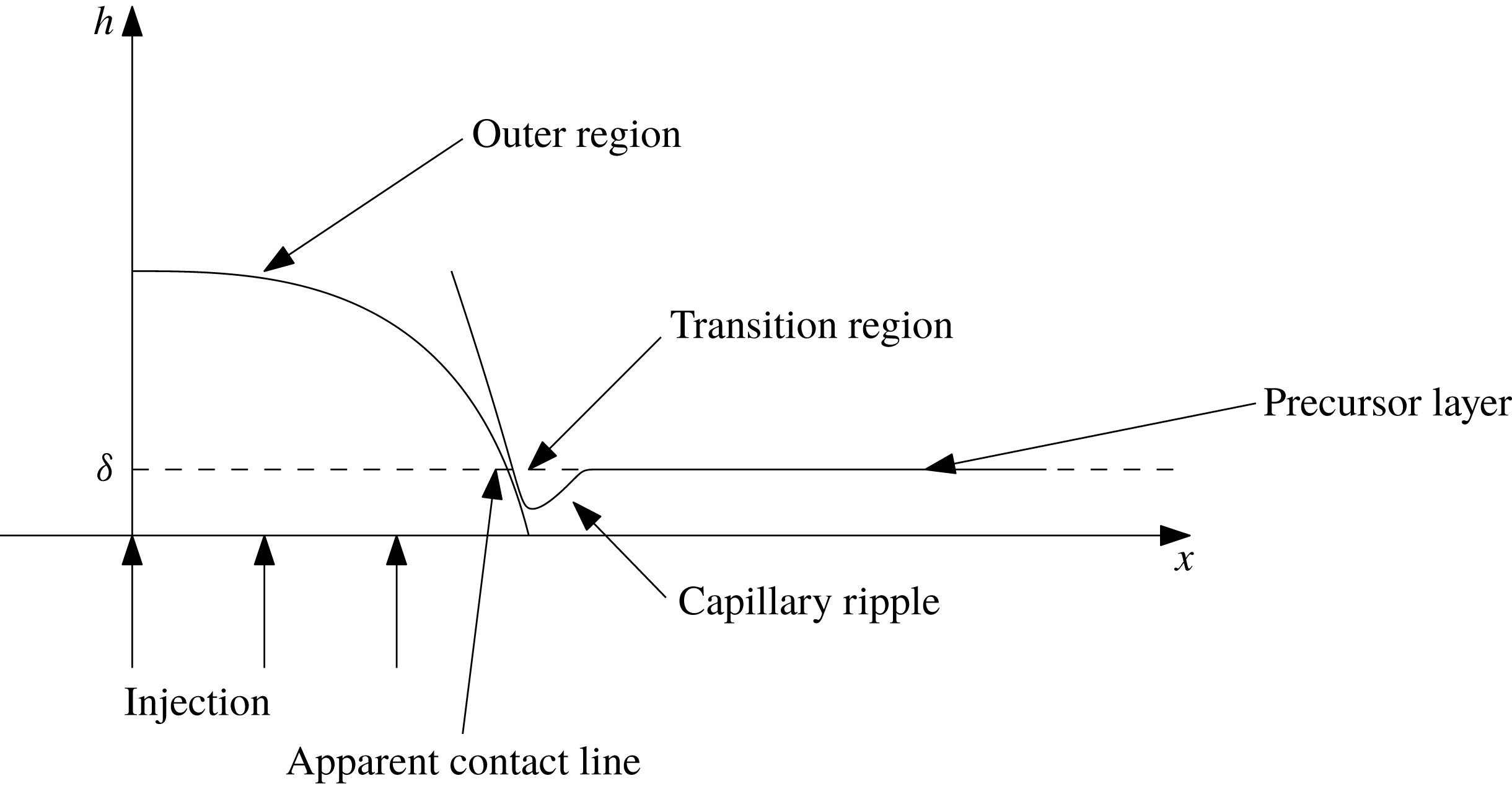
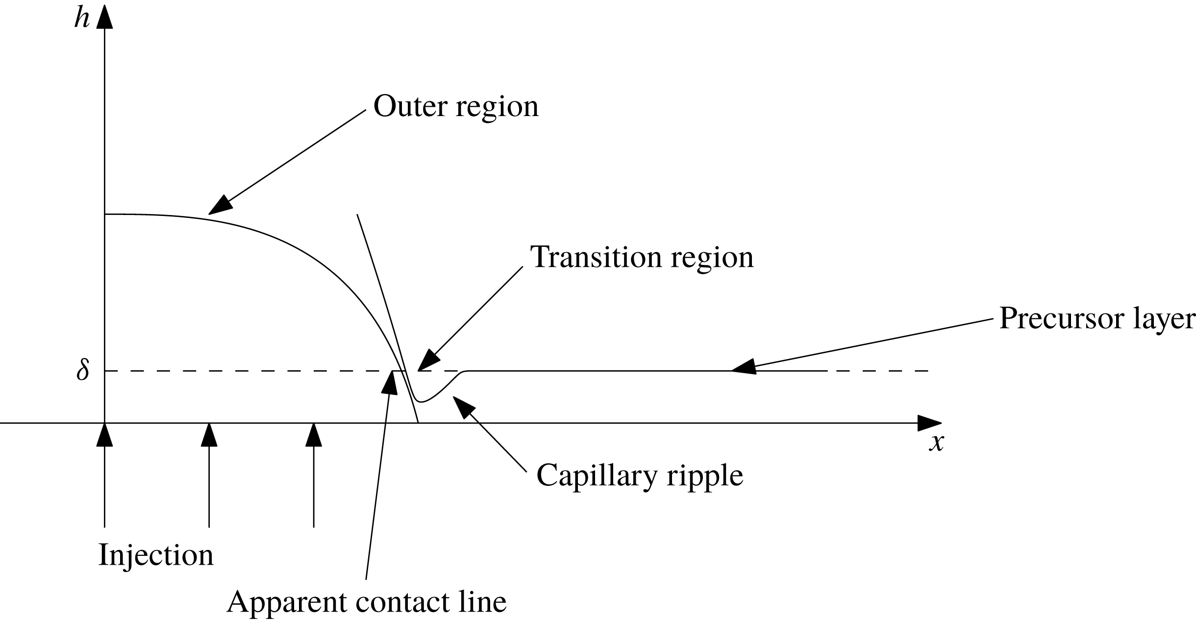
To explore the late-time behaviour of the system, we will rescale both time and the film thickness appropriately to arrive at a limit in which the surface-tension term in (2.23) is the only dominant term at leading order in the relevant asymptotic parameter (which will be determined as part of the analysis). This leading-order problem constitutes the solution in an outer region, the region to the left of the moving apparent contact line (see figure 3). At this stage, though, the position of the apparent contact line is an unknown function of time. We will solve for the film thickness in the transition region near the apparent contact line and match the solutions from the outer, transition and precursor-layer regions to obtain the full profile of the film thickness and the leading-order solution for the location of the moving boundary
 $a(t)$
. We will also see at the end of this section, and in § 5, that the late-time behaviour of our model is a generalization of the classical droplet-spreading problem when we allow the volume of liquid to be time dependent. However, unlike the classical droplet-spreading problem, we will obtain unbounded growth of the film, which is entirely due to the finite-width injection region. In § 5 we will consider some generalizations to our injection-spreading problem, and we will see that unbounded growth is not always guaranteed and depends on the functional form of the injection rate.
A schematic diagram of the outer, transition and precursor-layer regions, and the position of the apparent contact line. The film thicknesses are not drawn to scale.
3.3.1 The outer region
Unlike the spreading-droplet scenario considered in King & Bowen (Reference King and Bowen2001), here we anticipate that the injection results in a film thickness that is much larger than
 $\unicode[STIX]{x1D6FF}$
for late time. Thus, we scale
 $$\begin{eqnarray}t=\frac{\bar{t}}{\unicode[STIX]{x1D706}},\quad h=\frac{\bar{h}}{\unicode[STIX]{x1D706}},\end{eqnarray}$$
where
 $\unicode[STIX]{x1D706}=\unicode[STIX]{x1D706}(\unicode[STIX]{x1D6FF})\ll 1$
is to be determined. We note that we do not scale
 $x$
, because we anticipate that
 $a$
will move by an
 $O(1)$
amount on this time scale. After rearranging, equation (2.23) becomes
 $$\begin{eqnarray}\unicode[STIX]{x1D706}^{4}{\displaystyle \frac{\unicode[STIX]{x2202}\bar{h}}{\unicode[STIX]{x2202}\bar{t}}}+\frac{1}{3}{\displaystyle \frac{\unicode[STIX]{x2202}}{\unicode[STIX]{x2202}x}}\left(\bar{h}^{3}{\displaystyle \frac{\unicode[STIX]{x2202}^{3}\bar{h}}{\unicode[STIX]{x2202}x^{3}}}\right)=\unicode[STIX]{x1D706}^{4}\unicode[STIX]{x1D6E9}(1-x).\end{eqnarray}$$
The surface-tension term in (3.25) is dominant to leading order in
 $\unicode[STIX]{x1D706}^{4}$
. We assume
 $\unicode[STIX]{x1D6FF}\ll \unicode[STIX]{x1D706}^{4}\ll 1$
as
 $\unicode[STIX]{x1D6FF}\rightarrow 0$
, and will verify this assertion a posteriori. Expanding the dependent variables as
 $$\begin{eqnarray}\displaystyle & \bar{h}(x,\bar{t})\sim \bar{h}_{0}(x,\bar{t})+\unicode[STIX]{x1D706}^{4}\bar{h}_{1}(x,\bar{t})+\cdots \quad \text{as }\unicode[STIX]{x1D706}\rightarrow 0, & \displaystyle\end{eqnarray}$$
 $$\begin{eqnarray}\displaystyle & a(\bar{t})\sim a_{0}(\bar{t})+\unicode[STIX]{x1D706}^{4}a_{1}(\bar{t})+\cdots \quad \text{as }\unicode[STIX]{x1D706}\rightarrow 0, & \displaystyle\end{eqnarray}$$
the leading-order problem becomes
 $$\begin{eqnarray}{\displaystyle \frac{\unicode[STIX]{x2202}}{\unicode[STIX]{x2202}x}}\left(\bar{h}_{0}^{3}{\displaystyle \frac{\unicode[STIX]{x2202}^{3}\bar{h}_{0}}{\unicode[STIX]{x2202}x^{3}}}\right)=0,\end{eqnarray}$$
with
 $$\begin{eqnarray}\displaystyle & \displaystyle {\displaystyle \frac{\unicode[STIX]{x2202}\bar{h}_{0}}{\unicode[STIX]{x2202}x}}={\displaystyle \frac{\unicode[STIX]{x2202}^{3}\bar{h}_{0}}{\unicode[STIX]{x2202}x^{3}}}=0\quad \text{at }x=0, & \displaystyle\end{eqnarray}$$
 $$\begin{eqnarray}\displaystyle & \bar{h}_{0}=0\quad \text{at }x=a_{0}(\bar{t}). & \displaystyle\end{eqnarray}$$
The leading-order version of the conservation-of-mass equation (2.27) becomes
 $$\begin{eqnarray}\bar{t}=\int _{0}^{a_{0}(\bar{t})}\bar{h}_{0}(x,\bar{t})\,\text{d}x.\end{eqnarray}$$
Equation (3.28) with conditions (3.29)–(3.31) has a parabolic solution, namely,
 $$\begin{eqnarray}\bar{h}_{0}(x,\bar{t})=\frac{3\bar{t}(a_{0}^{2}-x^{2})}{2a_{0}^{3}},\end{eqnarray}$$
where
 $a_{0}(\bar{t})$
is unknown. In order to determine
 $a_{0}(\bar{t})$
, we will explore the solution in the transition region near the moving boundary and then match to (3.32).
3.3.2 The transition region
In the transition region near the moving front, we write
 $$\begin{eqnarray}t=\frac{\bar{t}}{\unicode[STIX]{x1D706}},\quad x=a_{0}(\bar{t})+\unicode[STIX]{x1D708}s(\bar{t})\unicode[STIX]{x1D709},\quad h=\unicode[STIX]{x1D6FF}H,\end{eqnarray}$$
where
 $\unicode[STIX]{x1D708}\ll 1$
, and we set
 $s(\bar{t})={\dot{a}}_{0}^{-1/3}$
for convenience in subsequent manipulations. With this change of variables, the spatial and time derivatives transform to
 $$\begin{eqnarray}{\displaystyle \frac{\unicode[STIX]{x2202}}{\unicode[STIX]{x2202}\bar{t}}}\rightarrow {\displaystyle \frac{\unicode[STIX]{x2202}}{\unicode[STIX]{x2202}\bar{t}}}-\left(\frac{{\dot{a}}_{0}}{\unicode[STIX]{x1D708}s}+\frac{\unicode[STIX]{x1D709}{\dot{s}}}{s}\right){\displaystyle \frac{\unicode[STIX]{x2202}}{\unicode[STIX]{x2202}\unicode[STIX]{x1D709}}},\quad {\displaystyle \frac{\unicode[STIX]{x2202}}{\unicode[STIX]{x2202}x}}\rightarrow \frac{1}{\unicode[STIX]{x1D708}s}{\displaystyle \frac{\unicode[STIX]{x2202}}{\unicode[STIX]{x2202}\unicode[STIX]{x1D709}}}.\end{eqnarray}$$
Furthermore, from § 3.2, we know that
 $a$
moves
 $O(1/\log (1/\unicode[STIX]{x1D6FF}))$
away from the end of the injection region for
 $O(1)$
time. Therefore, assuming that
 $\unicode[STIX]{x1D708}\ll 1/\log (1/\unicode[STIX]{x1D6FF})$
as
 $\unicode[STIX]{x1D6FF}\rightarrow 0$
(to be verified a posteriori), the transition region will lie outside the injection region for late time, and (2.23) becomes
 $$\begin{eqnarray}\unicode[STIX]{x1D706}\left(s^{4}{\displaystyle \frac{\unicode[STIX]{x2202}H}{\unicode[STIX]{x2202}\bar{t}}}-\left(\frac{1}{\unicode[STIX]{x1D708}}+\unicode[STIX]{x1D709}{\dot{s}}s^{3}\right){\displaystyle \frac{\unicode[STIX]{x2202}H}{\unicode[STIX]{x2202}\unicode[STIX]{x1D709}}}\right)+\frac{\unicode[STIX]{x1D6FF}^{3}}{3\unicode[STIX]{x1D708}^{4}}{\displaystyle \frac{\unicode[STIX]{x2202}}{\unicode[STIX]{x2202}\unicode[STIX]{x1D709}}}\left(H^{3}{\displaystyle \frac{\unicode[STIX]{x2202}^{3}H}{\unicode[STIX]{x2202}\unicode[STIX]{x1D709}^{3}}}\right)=0.\end{eqnarray}$$
In order to obtain a non-trivial dominant balance in (3.35), we balance the second and fourth terms, which requires that
 $$\begin{eqnarray}\unicode[STIX]{x1D708}=\frac{\unicode[STIX]{x1D6FF}}{\unicode[STIX]{x1D706}^{1/3}}.\end{eqnarray}$$
After rearranging, equation (3.35) then becomes
 $$\begin{eqnarray}\unicode[STIX]{x1D708}\left(s^{4}{\displaystyle \frac{\unicode[STIX]{x2202}H}{\unicode[STIX]{x2202}\bar{t}}}-\unicode[STIX]{x1D709}{\dot{s}}s^{3}{\displaystyle \frac{\unicode[STIX]{x2202}H}{\unicode[STIX]{x2202}\unicode[STIX]{x1D709}}}\right)-{\displaystyle \frac{\unicode[STIX]{x2202}H}{\unicode[STIX]{x2202}\unicode[STIX]{x1D709}}}+\frac{1}{3}{\displaystyle \frac{\unicode[STIX]{x2202}}{\unicode[STIX]{x2202}\unicode[STIX]{x1D709}}}\left(H^{3}{\displaystyle \frac{\unicode[STIX]{x2202}^{3}H}{\unicode[STIX]{x2202}\unicode[STIX]{x1D709}^{3}}}\right)=0.\end{eqnarray}$$
We expand the dependent variables in powers of
 $\unicode[STIX]{x1D708}=\unicode[STIX]{x1D708}(\unicode[STIX]{x1D6FF})$
, assuming
 $\unicode[STIX]{x1D6FF}\ll \unicode[STIX]{x1D708}\ll 1$
as
 $\unicode[STIX]{x1D6FF}\rightarrow 0$
, which we will also check a posteriori, and, thus, we write
 $$\begin{eqnarray}H(\unicode[STIX]{x1D709},\bar{t})\sim H_{0}(\unicode[STIX]{x1D709},\bar{t})+\unicode[STIX]{x1D708}H_{1}(\unicode[STIX]{x1D709},\bar{t})+\cdots \quad \text{as }\unicode[STIX]{x1D708}\rightarrow 0.\end{eqnarray}$$
Substituting (3.38) into (3.37), retaining leading-order terms, integrating once, and applying the matching condition with the precursor layer
 $$\begin{eqnarray}H_{0}\rightarrow 1\quad \text{as }\unicode[STIX]{x1D709}\rightarrow \infty ,\end{eqnarray}$$
we find that
 $H_{0}$
satisfies
 $$\begin{eqnarray}-H_{0}+\frac{1}{3}H_{0}^{3}{\displaystyle \frac{\unicode[STIX]{x2202}^{3}H_{0}}{\unicode[STIX]{x2202}\unicode[STIX]{x1D709}^{3}}}=-1.\end{eqnarray}$$
To match with the outer solution, we need to understand the behaviour of the transition-region solution as
 $\unicode[STIX]{x1D709}\rightarrow -\infty$
. We assume the solution is of the form
 $H_{0}\sim B(-\unicode[STIX]{x1D709})^{m}\log ^{n}(-\unicode[STIX]{x1D709}),$
as
 $\unicode[STIX]{x1D709}\rightarrow -\infty$
, for some values of
 $B,m$
and
 $n$
. Choosing
 $m=1$
,
 $n=1/3$
and
 $B=9^{1/3}$
gives the leading-order balance as
 $\unicode[STIX]{x1D709}\rightarrow -\infty$
between the two terms on the left-hand side of (3.40). Thus, our second matching condition is
 $$\begin{eqnarray}H_{0}\sim 9^{1/3}(-\unicode[STIX]{x1D709})\log ^{1/3}(-\unicode[STIX]{x1D709})\quad \text{as }\unicode[STIX]{x1D709}\rightarrow -\infty .\end{eqnarray}$$
We note that (3.40) has been solved by Duffy & Wilson (Reference Duffy and Wilson1997) for the case when the right-hand side is zero. Furthermore, they also obtain the asymptotic behaviour (3.41) (modulo the pre-factor), which confirms our result, since as
 $\unicode[STIX]{x1D709}\rightarrow -\infty$
,
 $H_{0}\rightarrow \infty$
and the right-hand side of (3.40), which is constant, does not appear in the dominant balance. We solve for
 $H_{0}$
using a shooting method. Specifically, we expand
 $H_{0}$
using
 $$\begin{eqnarray}H_{0}\sim 1+\tilde{H}_{0}\quad \text{as }\unicode[STIX]{x1D709}\rightarrow \infty ,\end{eqnarray}$$
where
 $\tilde{H}_{0}\ll 1$
. The equation for
 $\tilde{H}_{0}$
is
 $$\begin{eqnarray}\frac{1}{3}{\displaystyle \frac{\unicode[STIX]{x2202}^{3}\tilde{H}_{0}}{\unicode[STIX]{x2202}\unicode[STIX]{x1D709}^{3}}}-\tilde{H}_{0}=0,\end{eqnarray}$$
which has a solution that is a combination of exponentials. Retaining only decaying solutions and appropriately choosing the origin, we may write the solution as
 $$\begin{eqnarray}H_{0}\sim 1+\tilde{A}\exp (-3^{1/3}\unicode[STIX]{x1D709}/2)\cos (3^{5/6}\unicode[STIX]{x1D709}/2)\quad \text{as }\unicode[STIX]{x1D709}\rightarrow \infty .\end{eqnarray}$$
We then solve (3.40) by using
 $H_{0},H_{0}^{\prime },H_{0}^{\prime \prime }$
given by (3.44) evaluated at some large value of
 $\unicode[STIX]{x1D709}$
(we used
 $\unicode[STIX]{x1D709}=10$
);
 $\tilde{A}$
is our shooting parameter. We note that we can restrict the interval for possible values for
 $\tilde{A}$
to, for example,
 $[1,\exp (2\unicode[STIX]{x03C0}/\sqrt{3})]$
(McEwan & Taylor Reference McEwan and Taylor1966; Tuck & Schwartz Reference Tuck and Schwartz1990). We vary
 $\tilde{A}$
in order to match the behaviour as
 $\unicode[STIX]{x1D709}\rightarrow -\infty$
specified by (3.41). As in Tuck & Schwartz (Reference Tuck and Schwartz1990), we use the fact that
 $H_{0}H_{0}^{\prime }H_{0}^{\prime \prime }\rightarrow -3$
as
 $\unicode[STIX]{x1D709}\rightarrow -\infty$
to provide us with an accurate indicator of how close we are to the required solution.
3.3.3 Matching
We first match the transition region with the outer region. We write (3.41) in outer variables as
 $$\begin{eqnarray}\displaystyle \bar{h}_{0} & {\sim} & \displaystyle \frac{9^{1/3}\unicode[STIX]{x1D706}^{4/3}(a_{0}-x)\log ^{1/3}(\unicode[STIX]{x1D706}^{1/3}(a_{0}-x)/(\unicode[STIX]{x1D6FF}s))}{s}\nonumber\\ \displaystyle & {\sim} & \displaystyle \frac{9^{1/3}\unicode[STIX]{x1D706}^{4/3}(a_{0}-x)\log ^{1/3}(1/\unicode[STIX]{x1D6FF})}{s}\quad \text{as }\unicode[STIX]{x1D6FF}\rightarrow 0.\end{eqnarray}$$
The leading-order term in the outer solution (3.32) is
 $$\begin{eqnarray}\bar{h}_{0}\sim \frac{3\bar{t}(a_{0}-x)}{a_{0}^{2}}\quad \text{as }x\rightarrow a_{0}^{-}.\end{eqnarray}$$
This suggests that, to match (3.45) and (3.46), the appropriate scaling for
 $\unicode[STIX]{x1D706}$
should be
 $$\begin{eqnarray}\unicode[STIX]{x1D706}=\frac{1}{\log ^{1/4}(1/\unicode[STIX]{x1D6FF})}.\end{eqnarray}$$
Thus, equation (3.36) gives
 $$\begin{eqnarray}\unicode[STIX]{x1D708}=\unicode[STIX]{x1D6FF}\log ^{1/12}(1/\unicode[STIX]{x1D6FF}).\end{eqnarray}$$
We note that this confirms the hypotheses that
 $\unicode[STIX]{x1D6FF}\ll \unicode[STIX]{x1D708}\ll \unicode[STIX]{x1D706}^{4}\ll \unicode[STIX]{x1D706}\ll 1$
, as
 $\unicode[STIX]{x1D6FF}\rightarrow 0$
. Logarithmic scales also appear in similar problems described in Lacey (Reference Lacey1982), Hocking (Reference Hocking1983) and King & Bowen (Reference King and Bowen2001), for example. However, for the classical problem of a spreading droplet, the relevant scale is
 $1/\log (1/\unicode[STIX]{x1D6FF})$
(King & Bowen Reference King and Bowen2001), which is asymptotically smaller (in the limit
 $\unicode[STIX]{x1D6FF}\rightarrow 0$
) than our result (3.47) in the injection case. Matching (3.45) with (3.46), we obtain
 $$\begin{eqnarray}{\dot{a}}_{0}=\frac{3\bar{t\,}^{3}}{a_{0}^{6}},\end{eqnarray}$$
which can be solved to determine
 $a_{0}(\bar{t})$
. We also remark that (3.49) is a version of Tanner’s law, since it follows that, at the contact line,
 $$\begin{eqnarray}{\displaystyle \frac{\unicode[STIX]{x2202}\bar{h}_{0}}{\unicode[STIX]{x2202}x}}=-(9{\dot{a}}_{0})^{1/3}.\end{eqnarray}$$
We match the late-time behaviour for the contact line with the behaviour for
 $O(1)$
time, which results in imposing the initial condition
 $a_{0}\rightarrow 1$
as
 $t\rightarrow 0$
. Thus, equation (3.49) can be solved to yield
 $$\begin{eqnarray}a_{0}(\bar{t})=\left(1+\frac{21\bar{t\,}^{4}}{4}\right)^{1/7},\end{eqnarray}$$
and so,
 $$\begin{eqnarray}\bar{h}_{0}(0,\bar{t})=\frac{3\bar{t}}{2a_{0}}=\frac{3\bar{t}}{2}\left(1+\frac{21\bar{t\,}^{4}}{4}\right)^{-1/7}.\end{eqnarray}$$
In terms of the original variables,
 $h_{0}=\bar{h}_{0}/\unicode[STIX]{x1D706}$
and
 $t=\bar{t}/\unicode[STIX]{x1D706}$
,
 $$\begin{eqnarray}a_{0}(t)=\left(1+\frac{21\unicode[STIX]{x1D706}^{4}t^{4}}{4}\right)^{1/7},\quad h_{0}(0,t)=\frac{3t}{2}\left(1+\frac{21\unicode[STIX]{x1D706}^{4}t^{4}}{4}\right)^{-1/7}\quad \text{for }t=O(1/\unicode[STIX]{x1D706}).\quad\end{eqnarray}$$
We observe that, for late time, the apparent contact line moves much faster (
 ${\sim}t^{4/7}$
) than the classical non-injection case (
 ${\sim}t^{1/7}$
) considered in King & Bowen (Reference King and Bowen2001). We also note that, through
 $\unicode[STIX]{x1D706}$
, the leading-order results (3.53) have a dependence on the precursor thickness,
 $\unicode[STIX]{x1D6FF}$
. In physical systems where precursor layers are not observed,
 $\unicode[STIX]{x1D6FF}$
can be treated as an adjustable parameter to be determined from experimental data.
As mentioned at the beginning of § 3, we can generalize the results from the classical droplet-spreading problem (see, for example, Voinov Reference Voinov1976; Cox Reference Cox1986; Bonn et al.
Reference Bonn, Eggers, Indekeu, Meunier and Rolley2009) to the case of a time-dependent injection rate using the Cox–Voinov law (Bonn et al.
Reference Bonn, Eggers, Indekeu, Meunier and Rolley2009) to obtain the full late-time (
 $t\gg 1/\unicode[STIX]{x1D706}$
) behaviour of the film spreading (see appendix C for details).
We further note that we can also obtain the power-law dependence on time in (3.53) using scaling arguments. The matching condition (3.49) can also simply be deduced from a comparison of the slopes of
 $h$
in the inner and outer regions obtained from (3.45) and (3.46), respectively. Scaling
 $x\sim a$
, the slope of the outer solution
 ${\sim}h/a\sim t/a^{2}$
from (3.32), while the inner region has height
 ${\sim}\unicode[STIX]{x1D6FF}$
and length
 ${\sim}\unicode[STIX]{x1D6FF}{\dot{a}}^{-1/3}$
from (3.33) (with
 $\unicode[STIX]{x1D706}=1$
) and, thus, has slope
 $t/a^{2}\sim {\dot{a}}^{1/3}$
confirming the scalings
 $a\sim t^{4/7}$
and
 $h\sim t^{3/7}$
. Furthermore, if we look for a similarity solution to the problem for late time (essentially, away from the injection region) of the form
 $t^{\unicode[STIX]{x1D6FC}}f(x/t^{\unicode[STIX]{x1D6FD}})$
, for some exponents
 $\unicode[STIX]{x1D6FC}$
and
 $\unicode[STIX]{x1D6FD}$
, we can recover
 $\unicode[STIX]{x1D6FC}=3/7$
and
 $\unicode[STIX]{x1D6FD}=4/7$
and the parabolic profile for the outer solution. This, as we saw, is confirmed by the late-time asymptotic analysis. Thus, for late time the aspect ratio given by
 $h_{0}(0,t)/a_{0}(t)\sim t^{-1/7}$
, so remains small for all time.
4 Numerical results and discussion
We now present numerical solutions to the system (2.23)–(2.26). We approximate the boundary condition (2.25) by imposing
 $$\begin{eqnarray}\displaystyle & h=\unicode[STIX]{x1D6FF}\quad \text{on }x=l, & \displaystyle\end{eqnarray}$$
 $$\begin{eqnarray}\displaystyle & \displaystyle {\displaystyle \frac{\unicode[STIX]{x2202}h}{\unicode[STIX]{x2202}x}}=0\quad \text{on }x=l, & \displaystyle\end{eqnarray}$$
where
 $l$
is some large number. We used
 $l=60$
.
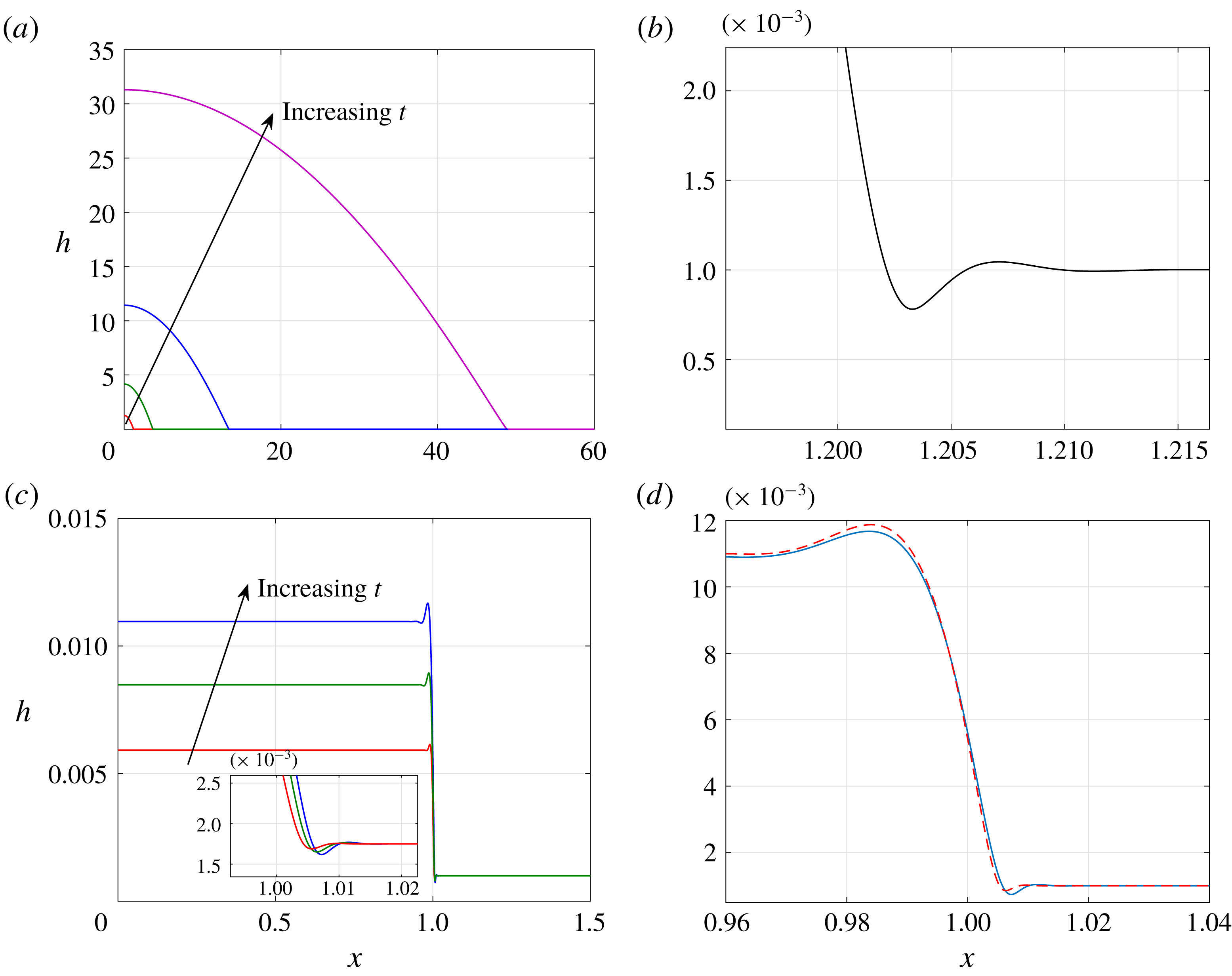
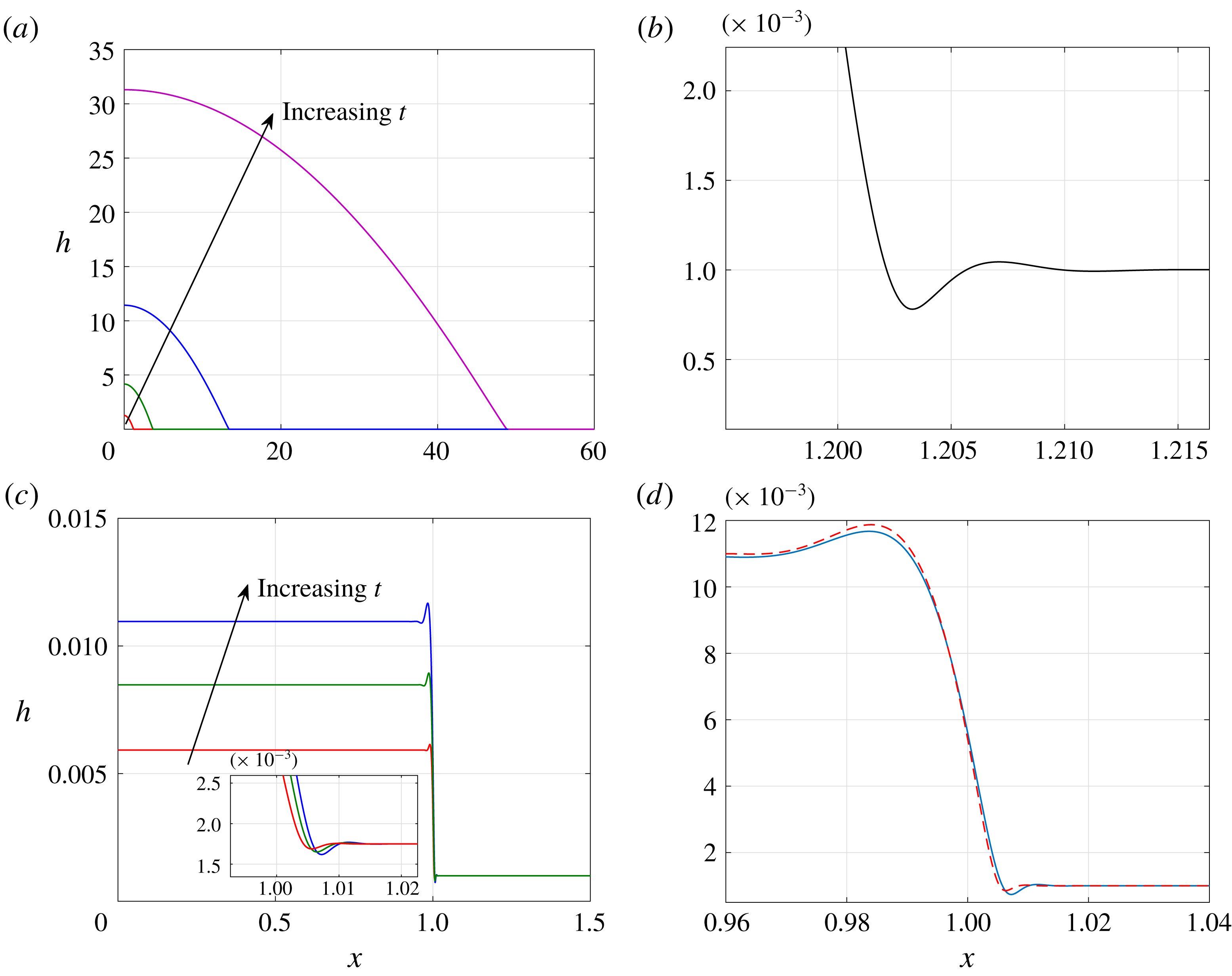
We employ a transformation of the coordinates that yields an adaptive mesh, which allows us to solve the problem for large time for a moderate computational cost (see appendix A for details). We solve the problem using MATLAB with a linear implicit Euler scheme. In figure 4(a), we show the numerical solutions for the spatial profile of the thickness
 $h(x,t)$
for various times where we have imposed a dimensionless precursor-layer thickness of
 $\unicode[STIX]{x1D6FF}=10^{-3}$
. As anticipated, the film thickness increases with time, and the front advances. We observe that the solutions appear self-similar, which indeed is the case for late time as found at the end of § 3.3.3. In figure 4(b), we show a zoom-in of the height profile near the apparent contact line, where we see characteristic capillary ripples. In figure 4(c), we show the numerical solutions for the spatial profile of the thickness
 $h(x,t)$
for various early times with a zoom-in of the apparent contact line near
 $x=1$
. We see that capillary ripples form on either side of
 $x=1$
and subsequently travel outwards in both directions. In § 3.1, we formulated the boundary-layer problem (3.8)–(3.11) for the transition between the spatially uniform solutions for early time given in (3.6). In figure 4(d), we show a plot of the film height near
 $x=1$
, found by solving (3.8)–(3.11) numerically, compared with the full numerical solution. We see good agreement between the two solutions.
In figure 5, we compare the thickness profile of the film at time
 $t=10$
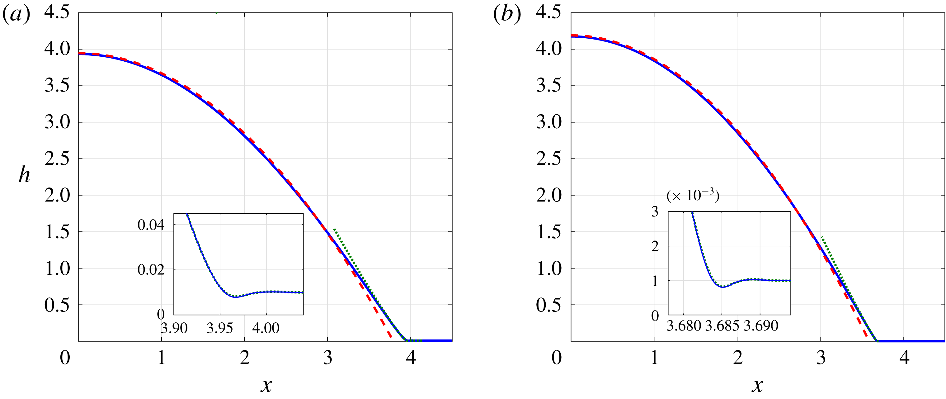
with the asymptotic predictions for late time for the outer- and transition-region profiles, given by (3.32) and (3.40) respectively, for two different precursor-layer thicknesses. We see excellent agreement between the numerical solution and the asymptotic solution as
 $\unicode[STIX]{x1D6FF}$
decreases. We have shifted the asymptotic solution for the inner region to allow for a detailed comparison with the numerical solution near the capillary ripple. This is shown in the small panels in the figures. In general, the positions of
 $x=a$
for the outer and inner regions are expected to differ, because the corrections to the leading-order outer solution for
 $a$
are large compared to the length scale of the inner region. We note that the predicted convergence is quite slow since our asymptotic sequence for
 $h(x,t)$
is logarithmic in nature. This slow logarithmic convergence is also present when slip regularization is used (see, for example, Lacey Reference Lacey1982; Hocking Reference Hocking1983).
Plots of the film thickness,
 $h(x,t)$
, satisfying (2.23)–(2.26) (a) at
 $t=1$
(red),
 $t=10$
(green),
 $t=100$
(blue),
 $t=1000$
(purple), (b) near
 $h=\unicode[STIX]{x1D6FF}$
and
 $x=1.2$
for
 $t=1$
and (c) at
 $t=0.005$
(red),
 $t=0.0075$
(green),
 $t=0.01$
(blue). In (d), we show the film thickness (solid blue) along with the solution to (3.8)–(3.11) (dashed red) near
 $x=1$
for
 $t=0.01$
. In all panels,
 $\unicode[STIX]{x1D6FF}=10^{-3}$
.
Plots of the film thickness,
 $h$
, satisfying (2.23)–(2.26), at
 $t=10$
: numerical solution (solid blue), asymptotic solution in the outer region (3.32) (dashed red), asymptotic solution in the transition region (3.40) (dotted green) for (a)
 $\unicode[STIX]{x1D6FF}=10^{-2}$
and (b)
 $\unicode[STIX]{x1D6FF}=10^{-3}$
.

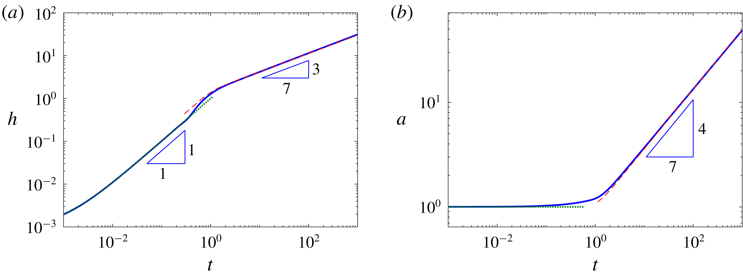
In figure 6, we show log–log plots of
 $h(0,t)$
and the position of the apparent contact line,
 $a(t)$
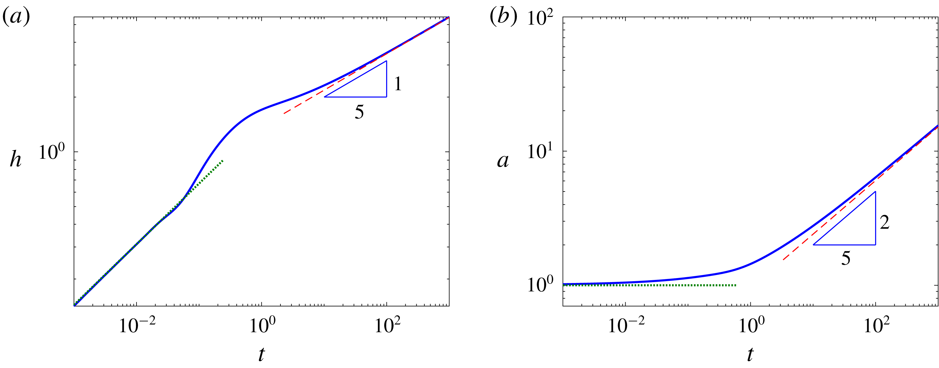
, given by the numerical solution to (2.23)–(2.26), together with our asymptotic predictions for early time, equation (3.6), and late time, equations (3.51)–(3.52). The asymptotic solutions match well for the early and late time behaviours, and, in fact, are valid for a much wider range of times than expected. We also note that the contact line does not move to leading order in
 $\unicode[STIX]{x1D6FF}$
for early time, as shown in § 3.1, and moves
 $O(1/\log (1/\unicode[STIX]{x1D6FF}))$
for
 $O(1)$
time, as shown in § 3.2.


5 General injection rates
In this section, we extend the model to the case of non-constant injection by replacing (2.4) with
 $$\begin{eqnarray}{\hat{w}}=\hat{f}(\hat{x},\hat{t})\unicode[STIX]{x1D6E9}(L-\hat{x})\quad \text{on }\hat{z}=0,\end{eqnarray}$$
for some dimensional supply function
 $\hat{f}(\hat{x},\hat{t})$
.
5.1 Power-law injection
We first consider the case in which
 $\hat{f}$
has a power-law dependence in time, i.e.
 $\hat{f}=\hat{t}^{k}{\hat{g}}(\hat{x})$
, where
 ${\hat{g}}$
is some integrable function on
 $[0,1]$
, and
 $k$
is some real exponent whose range we will specify later on. We expect that
 $k<0$
for physically sensible models, such as a chemical reaction whose rate decreases with time. However, we will also study the case
 $k>0$
. We note that, for
 $-1<k<0$
, the injection rate is singular at
 $t=0$
, but the volume of liquid (which is the time integral of the flux) is still finite. The case
 $k\leqslant -1$
corresponds to an infinite volume of liquid injected at
 $t=0$
, which we exclude on physical grounds. For simplicity, in the following analysis we assume that
 ${\hat{g}}=W$
is constant, even though more general spatial variance could be incorporated using the same approach. Thus, the boundary condition on the surface
 $\hat{z}=0$
becomes
 $$\begin{eqnarray}{\hat{w}}=W\hat{t}^{k}\unicode[STIX]{x1D6E9}(L-\hat{x})\quad \text{on }\hat{z}=0.\end{eqnarray}$$
In this case, we require a different non-dimensionalization and we use
 $$\begin{eqnarray}\left.\begin{array}{@{}c@{}}(\hat{x},\hat{a})=L(x,a),\quad (\hat{z},{\hat{h}})=(\unicode[STIX]{x1D707}W^{1/(k+1)}L^{4}/\unicode[STIX]{x1D6FE})^{(k+1)/(3k+4)}(z,h),\\ \hat{u} =(\unicode[STIX]{x1D6FE}W^{3}L^{3k}/\unicode[STIX]{x1D707})^{1/(3k+4)}u,\quad {\hat{w}}=(\unicode[STIX]{x1D707}W^{4/k}L^{4}/\unicode[STIX]{x1D6FE})^{k/(3k+4)}w,\\ \hat{t}=(\unicode[STIX]{x1D707}L^{4}/\unicode[STIX]{x1D6FE}W^{3})^{1/(3k+4)}t,\quad \hat{p}=(\unicode[STIX]{x1D707}^{k+1}\unicode[STIX]{x1D6FE}^{2k+3}W/L^{2k+4})^{1/(3k+4)}p.\end{array}\right\}\end{eqnarray}$$
We assume a long and thin geometry, i.e. that the aspect ratio
 $$\begin{eqnarray}\unicode[STIX]{x1D716}=(\unicode[STIX]{x1D707}W^{1/(k+1)}L^{k/k+1}/\unicode[STIX]{x1D6FE})^{(k+1)/(3k+4)}\ll 1,\end{eqnarray}$$
and that we have a thin precursor film, i.e.
 $\unicode[STIX]{x1D6FF}=h_{\infty }/(\unicode[STIX]{x1D716}L)\ll 1$
. Following the same steps as in § 2.2, we manipulate the dimensionless versions of (2.1)–(2.3), (2.5)–(2.7) and (5.2) and we arrive at the evolution equation for
 $h$
, namely
 $$\begin{eqnarray}{\displaystyle \frac{\unicode[STIX]{x2202}h}{\unicode[STIX]{x2202}t}}+\frac{1}{3}{\displaystyle \frac{\unicode[STIX]{x2202}}{\unicode[STIX]{x2202}x}}\left(h^{3}{\displaystyle \frac{\unicode[STIX]{x2202}^{3}h}{\unicode[STIX]{x2202}x^{3}}}\right)=t^{k}\unicode[STIX]{x1D6E9}(1-x),\end{eqnarray}$$
together with the boundary conditions given by (2.24)–(2.26).
For early time, we use a scaling similar to (3.1), but take account of the exponent
 $k$
in the injection function by setting
 $$\begin{eqnarray}h=\unicode[STIX]{x1D6FF}\tilde{h},\quad t=\unicode[STIX]{x1D6FF}^{1/(k+1)}\tilde{t},\end{eqnarray}$$
where, here, we restrict ourselves to considering
 $k>-1$
so that the scalings are valid for early time. After asymptotically expanding
 $h$
and
 $a$
in powers of
 $\unicode[STIX]{x1D6FF}$
as before, we arrive at a dominant balance between the first and third term in (5.5). Using the same notation as in § 3, we obtain
 $$\begin{eqnarray}\tilde{h}_{0}(x,\tilde{t})=1+\displaystyle \frac{\tilde{t}^{k+1}}{k+1}\unicode[STIX]{x1D6E9}(1-x).\end{eqnarray}$$
As in § 3.1, it is possible to obtain a problem for the boundary layer near
 $x=1$
, analogous to (3.8)–(3.11), which smoothly joins the two solutions given in (5.7), but we do not pursue that here. Instead, we point out that we can consider two distinct temporal regimes in which more analytical progress can be made (see appendix B for the details of this analysis).
For late time, we scale
 $$\begin{eqnarray}h=\frac{\bar{h}}{\unicode[STIX]{x1D706}_{k}},\quad t=\frac{\bar{t}}{\unicode[STIX]{x1D706}_{k}^{1/(k+1)}},\end{eqnarray}$$
where we assume
 $\unicode[STIX]{x1D706}_{k}\ll 1$
. Repeating the analysis in § 3.3, we find the appropriate choice of
 $\unicode[STIX]{x1D706}_{k}$
is (cf. (3.47))
 $$\begin{eqnarray}\unicode[STIX]{x1D706}_{k}=\frac{1}{\log ^{(k+1)/(3k+4)}(1/\unicode[STIX]{x1D6FF})},\end{eqnarray}$$
which is indeed small for
 $k>-1$
. Therefore, we obtain the following leading-order results for the position of the apparent contact line and the maximum film thickness
 $$\begin{eqnarray}\displaystyle & \displaystyle a_{0}(\bar{t})=\left(1+\frac{21\bar{t}^{\,3k+4}}{(k+1)^{3}(3k+4)}\right)^{1/7}, & \displaystyle\end{eqnarray}$$
 $$\begin{eqnarray}\displaystyle & \displaystyle \bar{h}_{0}(0,\bar{t})=\frac{3\bar{t}^{\,k+1}}{2(k+1)a_{0}}=\frac{3\bar{t}^{\,k+1}}{2(k+1)}\left(1+\frac{21\bar{t}^{\,3k+4}}{(k+1)^{3}(3k+4)}\right)^{-1/7}. & \displaystyle\end{eqnarray}$$
In an analogous way to § 3, we can use the Cox–Voinov law to obtain the full late-time behaviour of the film spreading when
 $t\gg 1/\unicode[STIX]{x1D706}_{k}^{1/(k+1)}$
.
We note that, in the case when
 $k=0$
, we recover the results (3.51) and (3.52). Furthermore, when
 $k=-3/4$
,
 $\bar{h}_{0}$
tends to a constant, i.e. injection is just enough to balance the surface-tension flow. Consequently, for
 $-1<k<-3/4$
, injection can no longer support a growing or constant film thickness, and, thus, the film thickness decreases at large time. For very large time, we expect capillarity to force the film to approach the thickness of the precursor layer again, and, thus, using the scaling from (5.11),
 $h\sim t^{(4k+3)/7}$
gives
 $t=\unicode[STIX]{x1D6FF}^{7/(4k+3)}t^{\star }$
as the required scaling for
 $t$
. We note that the same scaling can be derived from the balance
 $h-\unicode[STIX]{x1D6FF}\sim t^{k+1}/x,x\sim (\unicode[STIX]{x1D6FF}^{3}t)^{1/4}$
between the growth and the surface-tension term in (5.5). We do not pursue this situation further.
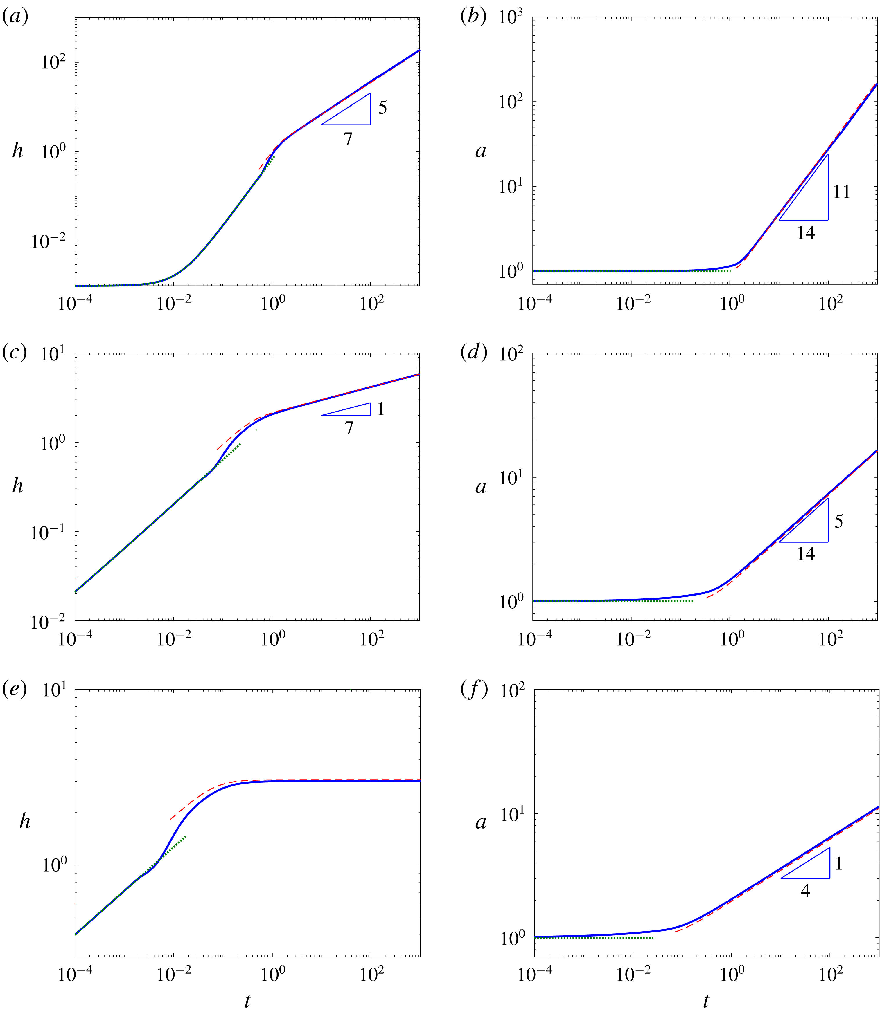
In figure 7, we show log–log plots of the numerical solution and our asymptotic predictions for the maximum film thickness at the origin and the position of the apparent contact line as functions of time for different values of
 $k$
. We see a good agreement between the numerical solution and the asymptotic results for early and late time.
Additionally, we observe that the aspect ratio, given by
 $h_{0}(0,t)/a_{0}(t)\sim t^{(k-1)/7}$
, grows in time if
 $k>1$
. In this case, for late time, the thin-film hypothesis will eventually break down.
Log–log plots of the numerical solution to (5.5) with (2.24)–(2.26) (solid blue) for
 $h(0,t)$
(a,c,e) and
 $a(t)$
(b,d,f) for (a,b)
 $k=1/2$
, (c,d)
 $k=-1/2$
, (e,f)
 $k=-3/4$
. The asymptotic predictions for early time, equation (5.7) (dotted green), and late time, equations (5.10)–(5.11) (dashed red), are also shown. In all figures,
 $\unicode[STIX]{x1D6FF}=10^{-3}$
.

Finally, we note that the results (5.10)–(5.11) can be used in a simple inverse problem, in which we can determine the exponent of the injection rate, assuming it has a power-law dependence, by observing the spreading of the film front or the evolution of its maximum thickness at the origin for late time. Thus, if the film front is observed to spread like
 $t^{\unicode[STIX]{x1D70E}}$
for some exponent
 $\unicode[STIX]{x1D70E}$
, then the exponent of the injection rate is given by
 $k=(7\unicode[STIX]{x1D70E}-4)/3$
. For example, if experimental data reveal a linear spread of the film front, then the liquid is also injected linearly in time.
5.2 Point-source injection
We now consider the case when liquid is injected at the origin, i.e. a point-source injection with
 $\hat{f}=Q\unicode[STIX]{x1D6FF}(\hat{x})$
in (5.1), where
 $Q$
is a given liquid flux. We note that, due to the definition of the delta function,
 $Q=2WL$
in terms of the notation in § 3. The boundary condition on
 $\hat{z}=0$
then becomes
 $$\begin{eqnarray}{\hat{w}}=Q\unicode[STIX]{x1D6FF}(\hat{x})\quad \text{on }\hat{z}=0.\end{eqnarray}$$
We non-dimensionalize using
 $$\begin{eqnarray}\left.\begin{array}{@{}c@{}}(\hat{x},\hat{a})=(\unicode[STIX]{x1D6FE}Q^{3}\unicode[STIX]{x1D70F}^{4}/\unicode[STIX]{x1D707})^{1/7}(x,a),\quad (\hat{z},{\hat{h}})=(\unicode[STIX]{x1D707}Q^{4}\unicode[STIX]{x1D70F}^{3}/\unicode[STIX]{x1D6FE})^{1/7}(z,h),\\ \hat{u} =(\unicode[STIX]{x1D6FE}Q^{3}/\unicode[STIX]{x1D707}\unicode[STIX]{x1D70F}^{3})^{1/7}u,\quad {\hat{w}}=(\unicode[STIX]{x1D707}Q^{4}/\unicode[STIX]{x1D6FE}\unicode[STIX]{x1D70F}^{4})^{1/7}w,\quad \hat{t}=\unicode[STIX]{x1D70F}t,\quad \hat{p}=(\unicode[STIX]{x1D707}^{3}\unicode[STIX]{x1D6FE}^{4}/Q^{2}\unicode[STIX]{x1D70F}^{5})^{1/7}p,\end{array}\right\}\end{eqnarray}$$
where we can choose the time scale
 $\unicode[STIX]{x1D70F}=(h_{\infty }^{7}\unicode[STIX]{x1D6FE}/\unicode[STIX]{x1D707}Q^{4})^{1/3}$
so that the dimensionless precursor-layer thickness
 $\unicode[STIX]{x1D6FF}=h_{\infty }(\unicode[STIX]{x1D707}Q^{4}\unicode[STIX]{x1D70F}^{3}/\unicode[STIX]{x1D6FE})^{-1/7}=1$
and we remove all dimensionless parameters from the model. However, we are interested in the situation where the film thickness is much larger than the precursor thickness and a long time scale over which the aspect ratio
 $\unicode[STIX]{x1D716}=\left(\unicode[STIX]{x1D707}^{2}Q/\unicode[STIX]{x1D6FE}^{2}\unicode[STIX]{x1D70F}\right)^{1/7}\ll 1$
so that the thin-film hypothesis is valid. Thus, we rescale our problem using
 $$\begin{eqnarray}t\rightarrow Tt,\quad (x,a)\rightarrow T^{4/7}(x,a),\quad (z,h)\rightarrow T^{3/7}(z,h)\end{eqnarray}$$
for some
 $T\gg 1$
. The evolution equation for
 $h$
becomes
 $$\begin{eqnarray}{\displaystyle \frac{\unicode[STIX]{x2202}h}{\unicode[STIX]{x2202}t}}+\frac{1}{3}{\displaystyle \frac{\unicode[STIX]{x2202}}{\unicode[STIX]{x2202}x}}\left(h^{3}{\displaystyle \frac{\unicode[STIX]{x2202}^{3}h}{\unicode[STIX]{x2202}x^{3}}}\right)=\unicode[STIX]{x1D6FF}(x),\end{eqnarray}$$
together with (2.24)–(2.26), in which the dimensionless precursor thickness now appears as
 $\unicode[STIX]{x1D6FF}=1/T^{3/7}\ll 1$
, and where we have used the fact that
 $\unicode[STIX]{x1D6FF}(\unicode[STIX]{x1D705}x)=\unicode[STIX]{x1D6FF}(x)/\unicode[STIX]{x1D705}$
for any
 $\unicode[STIX]{x1D705}>0$
. We note that, the thin-film hypothesis will hold as long as the new aspect ratio
 $\unicode[STIX]{x1D716}=\left(\unicode[STIX]{x1D707}^{2}Q/\unicode[STIX]{x1D6FE}^{2}\unicode[STIX]{x1D70F}T\right)^{1/7}\ll 1$
, which is true for sufficiently large
 $T$
. The appropriate limit of the late-time analysis presented in § 3.3 holds in this case too, since the width of the slot is asymptotically small for late time, and so, can be described by a delta function. We, thus, recover the power-law dependencies
 $$\begin{eqnarray}\displaystyle & \displaystyle a_{0}(\bar{t})=\left({\textstyle \frac{21}{32}}\right)^{1/7}\bar{t\,}^{4/7}, & \displaystyle\end{eqnarray}$$
 $$\begin{eqnarray}\displaystyle & \displaystyle \bar{h}_{0}(0,\bar{t})={\textstyle \frac{3}{4}}\left({\textstyle \frac{32}{21}}\right)^{1/7}\bar{t\,}^{3/7}, & \displaystyle\end{eqnarray}$$
where, again, we can use the Cox–Voinov law, as mentioned in § 3, to obtain the full late-time behaviour. However, we note that the numerical pre-factors are not the same as those in (3.51) and (3.52), since the strength of the source in this case is half that considered in § 3.3.
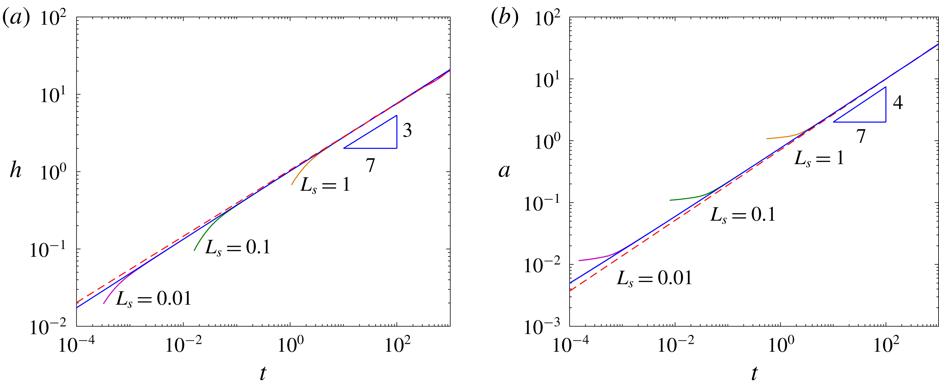
Log–log plots of the numerical solution to (5.19) with (5.20) and (2.25)–(2.26) (solid blue), the numerical solutions to (5.18) with (2.24)–(2.26) with
 $L_{s}=1$
(orange),
 $L_{s}=0.1$
(green) and
 $L_{s}=0.01$
(purple) for (a)
 $h(0,t)$
and (b)
 $a(t)$
, compared with the asymptotic predictions for late time (3.53) (dashed red). Here,
 $\unicode[STIX]{x1D6FF}=10^{-3}$
.

In figure 8, we show log–log plots of the maximum film thickness and the position of the apparent contact line as functions of time for the case of point-source injection. To simulate the behaviour of the delta function, we have used two approaches. First, we approximate a point-source injection using the original numerical solution with a finite injection slot of small width
 $\hat{L}_{s}=(\unicode[STIX]{x1D6FE}Q^{3}\unicode[STIX]{x1D70F}^{4}/\unicode[STIX]{x1D707})^{1/7}L_{s}$
, keeping the total flux of liquid constant by increasing the injection rate, i.e. replacing (5.15) with
 $$\begin{eqnarray}{\displaystyle \frac{\unicode[STIX]{x2202}h}{\unicode[STIX]{x2202}t}}+\frac{1}{3}{\displaystyle \frac{\unicode[STIX]{x2202}}{\unicode[STIX]{x2202}x}}\left(h^{3}{\displaystyle \frac{\unicode[STIX]{x2202}^{3}h}{\unicode[STIX]{x2202}x^{3}}}\right)=\frac{\unicode[STIX]{x1D6E9}(L_{s}-x)}{2L_{s}},\end{eqnarray}$$
where
 $L_{s}\ll 1$
. Second, we prescribe the flux at the origin by solving the problem
 $$\begin{eqnarray}{\displaystyle \frac{\unicode[STIX]{x2202}h}{\unicode[STIX]{x2202}t}}+\frac{1}{3}{\displaystyle \frac{\unicode[STIX]{x2202}}{\unicode[STIX]{x2202}x}}\left(h^{3}{\displaystyle \frac{\unicode[STIX]{x2202}^{3}h}{\unicode[STIX]{x2202}x^{3}}}\right)=0,\end{eqnarray}$$
subject to (2.25), (2.26), and
 $$\begin{eqnarray}{\displaystyle \frac{\unicode[STIX]{x2202}h}{\unicode[STIX]{x2202}x}}=0,\quad \frac{1}{3}h^{3}{\displaystyle \frac{\unicode[STIX]{x2202}^{3}h}{\unicode[STIX]{x2202}x^{3}}}=\frac{1}{2}\quad \text{at }x=0.\end{eqnarray}$$
We also plot the asymptotic results (5.16) and (5.17) across the entire
 $t$
range (despite them only being formally valid for
 $t\gg 1$
). We see a very good agreement between the numerical results obtained using the second approach and the asymptotic results for a wider range of time than anticipated. The asymptotic results provide a good estimate at early time, because, in this case, the slot has been shrunk to a point. For early time, we observe a slight discrepancy between the numerical and the asymptotic results, which can be explained by the finite precursor film, which is present everywhere on the substrate at
 $t=0$
and is not reflected by our ‘late-time’ results. We also see that, as time increases, the numerical solution from the first approach converges to the numerical solution from the second approach (as anticipated) and to the asymptotic predictions (5.16) and (5.17), and the time to convergence decreases as
 $L_{s}$
decreases. To illustrate this, we consider the early-time behaviour. As before, we determine the linear growth for early time by balancing the first and third terms in (5.18), which gives
 $$\begin{eqnarray}h=\unicode[STIX]{x1D6FF}+\frac{t}{L_{s}}\unicode[STIX]{x1D6E9}(L_{s}-x).\end{eqnarray}$$
We obtain the range of validity of the early-time solution (5.21) by requiring that the ‘discontinuous’ step that is initially at
 $x=L_{s}$
has not spread to the origin. By considering (5.21), we see that, if
 $t\ll \unicode[STIX]{x1D6FF}L_{s}$
, then
 $h\sim \unicode[STIX]{x1D6FF}$
, and the validity condition, found using a scaling argument on (5.19), reads
 $$\begin{eqnarray}(\unicode[STIX]{x1D6FF}^{3}t)^{1/4}\ll L_{s}.\end{eqnarray}$$
If
 $\unicode[STIX]{x1D6FF}L_{s}\ll t\ll 1$
, then
 $h\sim t/L_{s}$
from (5.21), and the validity condition is instead
 $$\begin{eqnarray}(h^{3}t)^{1/4}\ll L_{s}.\end{eqnarray}$$
The two conditions (5.22) and (5.23) can be combined into a single range of validity,
 $t\ll \min \{L_{s}^{4}/\unicode[STIX]{x1D6FF}^{3},L_{s}^{7/4}\}$
. We note that when
 $L_{s}=1$
, the validity condition becomes
 $t\ll 1$
, as seen in § 3.1.
6 Thickness-inhibited injection
A final regime of interest is one in which the rate of injection decreases as the liquid thickness grows. Such a scenario might arise when liquid forms through a chemical reaction on the surface, which requires the chemical to diffuse through the liquid film to reach the surface. This may be captured by considering a dimensional supply flux
 $W/{\hat{h}}^{q}$
, where
 $q>0$
is a constant. We note that the case
 $q=1$
corresponds to standard diffusion with flux inversely proportional to the thickness of the film. The boundary condition on
 $\hat{z}=0$
then becomes
 $$\begin{eqnarray}{\hat{w}}=\frac{W}{{\hat{h}}^{q}}\unicode[STIX]{x1D6E9}(L-\hat{x})\quad \text{on }\hat{z}=0.\end{eqnarray}$$
This time, we non-dimensionalize (2.1)–(2.3), (2.5)–(2.7) and (6.1) using
 $$\begin{eqnarray}\left.\begin{array}{@{}c@{}}(\hat{x},\hat{a})=L(x,a),\quad (\hat{z},{\hat{h}})=(\unicode[STIX]{x1D707}WL^{4}/\unicode[STIX]{x1D6FE})^{1/(q+4)}(z,h),\\ \hat{u} =(\unicode[STIX]{x1D6FE}^{q+1}W^{3}/\unicode[STIX]{x1D707}^{q+1}L^{3q})^{1/(q+4)}u,\quad {\hat{w}}=(\unicode[STIX]{x1D6FE}W^{4/q}/\unicode[STIX]{x1D707}L^{4})^{q/(q+4)}w,\quad \\ \hat{t}=(\unicode[STIX]{x1D707}L^{4}/\unicode[STIX]{x1D6FE}W^{3/(q+1)})^{(q+1)/(q+4)}t,\quad \hat{p}=(\unicode[STIX]{x1D707}\unicode[STIX]{x1D6FE}^{q+3}W/L^{2q+4})^{1/(q+4)}p.\end{array}\right\}\end{eqnarray}$$
We continue assuming a long and thin geometry, i.e. that the aspect ratio
 $$\begin{eqnarray}\unicode[STIX]{x1D716}=(\unicode[STIX]{x1D707}W/\unicode[STIX]{x1D6FE}L^{q})^{1/(q+4)}\ll 1,\end{eqnarray}$$
and that the precursor layer is thin, i.e.
 $\unicode[STIX]{x1D6FF}=h_{\infty }/(\unicode[STIX]{x1D716}L)\ll 1$
. The evolution equation for
 $h$
is then
 $$\begin{eqnarray}{\displaystyle \frac{\unicode[STIX]{x2202}h}{\unicode[STIX]{x2202}t}}+\frac{1}{3}{\displaystyle \frac{\unicode[STIX]{x2202}}{\unicode[STIX]{x2202}x}}\left(h^{3}{\displaystyle \frac{\unicode[STIX]{x2202}^{3}h}{\unicode[STIX]{x2202}x^{3}}}\right)=\frac{1}{h^{q}}\unicode[STIX]{x1D6E9}(1-x),\end{eqnarray}$$
For early time, we rescale the film thickness and time according to
 $$\begin{eqnarray}h=\unicode[STIX]{x1D6FF}\tilde{h},\quad t=\unicode[STIX]{x1D6FF}^{q+1}\tilde{t}.\end{eqnarray}$$
The leading-order (in
 $\unicode[STIX]{x1D6FF}$
) solution satisfies
 $$\begin{eqnarray}{\displaystyle \frac{\unicode[STIX]{x2202}\tilde{h}_{0}}{\unicode[STIX]{x2202}\tilde{t}}}=\frac{1}{\tilde{h}_{0}^{q}}\unicode[STIX]{x1D6E9}(1-x),\end{eqnarray}$$
with an initial condition given by
 $$\begin{eqnarray}\tilde{h}_{0}=1\quad \text{at }\tilde{t}=0.\end{eqnarray}$$
The solution to (6.6) with (6.7) has a power-law behaviour in
 $0\leqslant x\leqslant 1$
and is constant in
 $x>1$
, with
 $$\begin{eqnarray}\tilde{h}_{0}(x,\tilde{t})=(1+(q+1)\tilde{t}\unicode[STIX]{x1D6E9}(1-x))^{1/(q+1)}.\end{eqnarray}$$
A boundary-layer analysis near
 $x=1$
analogous to the one in § 3.1 provides a continuous solution smoothly joining the film thicknesses on either side of
 $x=1$
, but we do not examine it in this paper.
For late time, we scale
 $$\begin{eqnarray}h=\frac{\bar{h}}{\unicode[STIX]{x1D706}_{q}},\quad t=\frac{\bar{t}}{\unicode[STIX]{x1D706}_{q}^{q+1}},\end{eqnarray}$$
where we assume
 $\unicode[STIX]{x1D706}_{q}\ll 1$
. Repeating the analysis in § 3.3, we find the appropriate choice of
 $\unicode[STIX]{x1D706}_{q}$
is (cf. (3.47))
 $$\begin{eqnarray}\unicode[STIX]{x1D706}_{q}=\frac{1}{\log ^{1/(q+4)}(1/\unicode[STIX]{x1D6FF})},\end{eqnarray}$$
which is indeed small for
 $q>0$
. We note that the analogue of (3.31) is
 $$\begin{eqnarray}V(\bar{t})=\int _{0}^{\bar{t}}\int _{0}^{1}\frac{1}{\bar{h}_{0}^{q}(x,s)}\,\text{d}x\,\text{d}s=\int _{0}^{a_{0}(\bar{t})}\bar{h}_{0}(x,\bar{t})\,\text{d}x,\end{eqnarray}$$
where
 $V$
is the leading-order volume of the liquid.
Repeating the analysis in § 3.3, we obtain the outer solution for the leading-order film thickness,
 $\bar{h}_{0}$
 $$\begin{eqnarray}\bar{h}_{0}(x,\bar{t})=A(\bar{t})(a_{0}^{2}-x^{2}),\end{eqnarray}$$
where
 $A(\bar{t})$
satisfies
 $$\begin{eqnarray}A(\bar{t})=\frac{3V(\bar{t})}{2a_{0}(\bar{t})^{3}}=\frac{3}{2a_{0}(\bar{t})^{3}}\int _{0}^{\bar{t}}\int _{0}^{1}\frac{1}{A(s)^{q}(a_{0}^{2}(s)-x^{2})^{q}}\,\text{d}x\,\text{d}s.\end{eqnarray}$$
In this case, we end up with the following integro-differential equation for
 $a_{0}(\bar{t})$
 $$\begin{eqnarray}{\dot{a}}_{0}=\frac{8}{9}a_{0}^{3}A^{3}=\frac{3V^{3}}{a_{0}^{6}}=\frac{3}{a_{0}^{6}}\left(\int _{0}^{\bar{t}}\int _{0}^{1}\frac{1}{A(s)^{q}(a_{0}^{2}(s)-x^{2})^{q}}\,\text{d}x\,\text{d}s\right)^{3}.\end{eqnarray}$$
We note that setting
 $q=0$
recovers (3.49).
In order to make further analytical progress, we first transform (6.14) into an ordinary differential equation by differentiating both sides with respect to time and using (6.13). We then obtain
 $$\begin{eqnarray}\ddot{a}_{0}=-6\frac{{\dot{a}}_{0}^{2}}{a_{0}}+4\unicode[STIX]{x1D712}(\bar{t})\left(\frac{9{\dot{a}}_{0}}{8a_{0}^{3}}\right)^{(2-q)/3},\end{eqnarray}$$
where
 $$\begin{eqnarray}\unicode[STIX]{x1D712}(\bar{t\,})=\int _{0}^{1}\frac{1}{(a_{0}(\bar{t\,})^{2}-x^{2})^{q}}\,\text{d}x.\end{eqnarray}$$
Anticipating that
 $a_{0}\gg 1$
for large
 $\bar{t}$
, we can approximate (6.15) by
 $$\begin{eqnarray}\ddot{a}_{0}=-6\frac{{\dot{a}}_{0}^{2}}{a_{0}}+4\left(\frac{9{\dot{a}}_{0}}{8a_{0}^{3}}\right)^{(2-q)/3}\frac{1}{a_{0}^{2q}}.\end{eqnarray}$$
If we now try an ansatz of the form
 $a_{0}=C\bar{t\,}^{D}$
, for some constants
 $C,D$
, we find
 $$\begin{eqnarray}D=\frac{q+4}{4q+7},\quad C=\left(\frac{2^{3q}3^{1-2q}(4q+7)^{q+4}}{(q+4)^{q+1}(q+7)^{3}}\right)^{1/(4q+7)}.\end{eqnarray}$$
We, thus, obtain the power-law behaviour of the maximum film thickness and the position of the apparent contact line for
 $\bar{t}\gg 1$
 $$\begin{eqnarray}\displaystyle & \displaystyle \bar{h}_{0}(0,\bar{t})\sim \left(\frac{9(q+4)}{8(4q+7)}\right)^{1/3}C^{4/3}\bar{t\,}^{3/(4q+7)}, & \displaystyle\end{eqnarray}$$
 $$\begin{eqnarray}\displaystyle & a_{0}(\bar{t})\sim C\bar{t\,}^{(q+4)/(4q+7)}, & \displaystyle\end{eqnarray}$$
where
 $C$
is defined in (6.18). We see that setting
 $q=0$
recovers (3.51) and (3.52). We note that we can obtain the exponents of these power-law dependencies using the scaling arguments, found at the end of § 3. Also, as mentioned in § 3, it is possible to use the Cox–Voinov law in the case of thickness-dependent injection to obtain the true late-time behaviour of the film spreading. In particular, our results (6.19) and (6.20) are valid for
 $1\ll \bar{t}=\unicode[STIX]{x1D706}_{q}t\ll \unicode[STIX]{x1D706}_{q}/\unicode[STIX]{x1D6FF}^{(4q+7)/3}$
(cf. comment immediately after (C 5) with
 $q=0$
). We also remark that the aspect ratio for the problem is
 $\unicode[STIX]{x1D716}=h_{0}/a_{0}\sim t^{-(q+1)/(4q+7)}\ll 1$
for large
 $t$
and
 $q>0$
, and so, the thin-film hypothesis holds.
To illustrate our analysis for a particular value of
 $q$
, we take
 $q=2$
, for which (6.15) simplifies substantially, and we can perform the integration in (6.16):
 $$\begin{eqnarray}\int _{0}^{1}\frac{1}{(a_{0}^{2}-x^{2})^{2}}\,\text{d}x=\frac{(a_{0}^{2}-1)\coth ^{-1}(a_{0})-a_{0}}{2a_{0}^{3}(a_{0}^{2}-1)}\sim \frac{1}{a_{0}^{4}}\quad \text{for }a_{0}\gg 1.\end{eqnarray}$$
We then have
 $$\begin{eqnarray}\displaystyle & \displaystyle a_{0}(\bar{t})\sim \left({\textstyle \frac{50}{9}}\right)^{1/5}\bar{t\,}^{2/5}, & \displaystyle\end{eqnarray}$$
 $$\begin{eqnarray}\displaystyle & \displaystyle \bar{h}_{0}(0,\bar{t})\sim \left({\textstyle \frac{5\times 9^{1/3}}{4}}\right)^{1/5}\bar{t\,}^{1/5}. & \displaystyle\end{eqnarray}$$
In figure 9, we show log–log plots of the maximum film thickness and the position of the apparent contact line for the case of thickness-inhibited injection with
 $q=2$
. We see a very good agreement between the numerical solutions and the predicted asymptotic results for early time, given by (6.8), and late time, given by (6.22)–(6.23).


7 Conclusions and further work
In this paper, we have considered the problem of surface-tension-driven flow of a viscous liquid along a flat surface with injection through part of the substrate. Throughout our work, we assumed that gravity could be neglected. We initially focused on the situation in which the injection rate was constant. We derived a fourth-order parabolic evolution equation for the thickness profile, along with appropriate boundary conditions, reflecting the injection in a fixed region. We assumed that a thin precursor layer was present initially along the surface, which resolved the stress singularity at the moving contact line. We used asymptotic analysis for early,
 $O(1)$
, and late time in order to examine the behaviour of the solution, and obtained power-law dependencies on time for the maximum film thickness at the centre of the injection region,
 $h_{0}(0,t)$
, and the position of the apparent contact line,
 $a_{0}(t)$
. We recovered a version of Tanner’s law at the apparent contact line, namely,
 $\unicode[STIX]{x2202}h_{0}/\unicode[STIX]{x2202}x\propto -({\dot{a}}_{0})^{1/3}$
. For early time, we established a linear growth of the film thickness in the injection region and no movement of the contact line to leading order. We justified the absence of motion of the contact line to leading order for
 $O(1)$
time, while for late time,
 $t$
, the maximum film thickness scales as
 $t^{3/7}$
and the position of the apparent contact line scales as
 $t^{4/7}$
. Up to a multiplicative constant, the time-dependent aspect ratio is
 $h_{0}(0,t)/a_{0}(t)\sim t^{-1/7}$
, as
 $t\rightarrow \infty$
, which is consistent with the thin-film assumption. We observed that the leading-order results for
 $h$
and
 $a$
depend on the precursor thickness,
 $\unicode[STIX]{x1D6FF}$
. We also showed how to generalize classical results (such as the Cox–Voinov law) from the droplet-spreading problem in the case of injection to obtain the full late-time behaviour of the film.
Finally, we considered three generalizations to the problem: a power-law, point-source and thickness-dependent injection rate. In the first case, we looked at injection of the form
 $t^{k}$
with an exponent in the range
 $-1<k<1$
, and established power-law behaviours for the maximum film thickness and the position of the apparent contact line as functions of time. We showed that, for late time, the film thickness increased for
 $k>-3/4$
, tended to a constant for
 $k=-3/4$
, and decreased for
 $k<-3/4$
. For
 $k\geqslant 1$
, the aspect ratio of the problem grows unboundedly with time and eventually invalidates the thin-film hypothesis. We also presented a simple inverse problem for determining the exponent of the power-law injection (assuming this exists) by observing the position of the apparent contact line, for example. In the point-source case, we obtained the same late-time behaviour as in the constant-injection-rate case. With regards to the thickness-dependent injection, we formulated the problem with injection of the form
 $1/h^{q}$
for some exponent
 $q>0$
. We obtained an integro-differential equation for the position of the apparent contact line for late time and simplified it to an ordinary differential equation. We found power-law behaviours for the maximum thickness of the film and the position of the apparent contact line, which were confirmed using scaling arguments. Unlike the time-dependent injection case, we observed unbounded growth and spreading of the film for all
 $q>0$
. We note that, as
 $q$
increases, the exponents in the spreading behaviour decrease, corresponding to a slowing down of the film growth and front spreading. Furthermore, we see a close relationship between the behaviour for
 $a(t)$
and
 $h(0,t)$
between the power-law injection and the thickness-inhibited injection cases; they are identical if
 $k=-3q/(4q+7)$
. Interestingly, since
 $q>0$
,
 $k\rightarrow -3/4$
as
 $q\rightarrow \infty$
. This recovers the critical exponent for time-dependent injection at which the film thickness stops increasing for late time. This gives a relationship between the qualitative behaviours for late time of the maximum film thickness and the position of the apparent contact line with power-law-in-time and thickness-inhibited injection rates.
There are various key extensions to this work that we believe would be interesting. One would be to replace the flat substrate with a cylinder. This has the potential of introducing the well-known Rayleigh–Plateau instability, and a key question would be how the two principal curvatures affect the flow. Also of interest would be to study multiple fluid injection sites.
Our ultimate aim is to use the insight we have obtained by studying these surface-tension- and injection-driven flows to provide a better understanding of the operation of purification devices.
Acknowledgements
This publication is based on work partially supported by the EPSRC Centre For Doctoral Training in Industrially Focused Mathematical Modelling (EP/L015803/1) in collaboration with W. L. Gore and associates. We would like to thank U. Beuscher and V. Venkateshwaran from Gore for their crucial contributions. I.M.G. gratefully acknowledges support from the Royal Society through a University Research Fellowship. It is a pleasure to also thank D. Schwendeman, D. Vella and J. Oliver for invaluable discussions and comments. Finally, we are indebted to an anonymous referee for their insightful comments, which have significantly enhanced this paper.
Appendix A. A suitable change of coordinates for numerical solution
When solving numerically (2.23) together with (2.24)–(2.26), we employ the following coordinate transformation
 $$\begin{eqnarray}\unicode[STIX]{x1D702}=\frac{x}{t^{1/4}},\quad \unicode[STIX]{x1D70F}=\log (t).\end{eqnarray}$$
In terms of
 $\unicode[STIX]{x1D702}$
and
 $\unicode[STIX]{x1D70F}$
, our problem for
 $h(x,t)=F(\unicode[STIX]{x1D702},\unicode[STIX]{x1D70F})$
becomes
 $$\begin{eqnarray}{\displaystyle \frac{\unicode[STIX]{x2202}F}{\unicode[STIX]{x2202}\unicode[STIX]{x1D70F}}}-\frac{1}{4}\unicode[STIX]{x1D702}{\displaystyle \frac{\unicode[STIX]{x2202}F}{\unicode[STIX]{x2202}\unicode[STIX]{x1D702}}}+\frac{1}{3}{\displaystyle \frac{\unicode[STIX]{x2202}}{\unicode[STIX]{x2202}\unicode[STIX]{x1D702}}}\left(F^{3}{\displaystyle \frac{\unicode[STIX]{x2202}^{3}F}{\unicode[STIX]{x2202}\unicode[STIX]{x1D702}^{3}}}\right)=\text{e}^{\unicode[STIX]{x1D70F}}\unicode[STIX]{x1D6E9}(1-\text{e}^{\unicode[STIX]{x1D70F}/4}\unicode[STIX]{x1D702}),\end{eqnarray}$$
subject to
 $$\begin{eqnarray}\displaystyle & \displaystyle {\displaystyle \frac{\unicode[STIX]{x2202}F}{\unicode[STIX]{x2202}\unicode[STIX]{x1D702}}}={\displaystyle \frac{\unicode[STIX]{x2202}^{3}F}{\unicode[STIX]{x2202}\unicode[STIX]{x1D702}^{3}}}=0\quad \text{at }\unicode[STIX]{x1D702}=0, & \displaystyle\end{eqnarray}$$
 $$\begin{eqnarray}\displaystyle & F\rightarrow \unicode[STIX]{x1D6FF}\quad \text{as }\unicode[STIX]{x1D702}\rightarrow \infty , & \displaystyle\end{eqnarray}$$
 $$\begin{eqnarray}\displaystyle & F=\unicode[STIX]{x1D6FF}\quad \text{at }\unicode[STIX]{x1D70F}\rightarrow -\infty . & \displaystyle\end{eqnarray}$$
If we discretize this problem using an implicit linear Euler scheme and a sufficiently small time step, then our time domain for
 $\unicode[STIX]{x1D70F}$
is much smaller than that for
 $t$
due to the exponential nature of the transformation in time. Thus, enlarging the
 $\unicode[STIX]{x1D70F}$
-domain marginally gives a much greater increase in the
 $t$
-domain.
When solving the problem numerically, we require that the spatial step is bounded by the film height in order to ensure that the region near the capillary ripple is well resolved (Diez, Kondic & Bertozzi Reference Diez, Kondic and Bertozzi2001). Clearly, this presents computational issues as
 $\unicode[STIX]{x1D6FF}\rightarrow 0$
. We employ the transformation
 $$\begin{eqnarray}F=\text{e}^{G},\end{eqnarray}$$
and the problem for
 $G(\unicode[STIX]{x1D702},\unicode[STIX]{x1D70F})$
becomes
 $$\begin{eqnarray}{\displaystyle \frac{\unicode[STIX]{x2202}G}{\unicode[STIX]{x2202}\unicode[STIX]{x1D70F}}}-\frac{1}{4}\unicode[STIX]{x1D702}{\displaystyle \frac{\unicode[STIX]{x2202}G}{\unicode[STIX]{x2202}\unicode[STIX]{x1D702}}}+\frac{\text{e}^{-G}}{3}{\displaystyle \frac{\unicode[STIX]{x2202}}{\unicode[STIX]{x2202}\unicode[STIX]{x1D702}}}\left(\text{e}^{4G}\left(\left({\displaystyle \frac{\unicode[STIX]{x2202}G}{\unicode[STIX]{x2202}\unicode[STIX]{x1D702}}}\right)^{3}+3{\displaystyle \frac{\unicode[STIX]{x2202}G}{\unicode[STIX]{x2202}\unicode[STIX]{x1D702}}}{\displaystyle \frac{\unicode[STIX]{x2202}^{2}G}{\unicode[STIX]{x2202}\unicode[STIX]{x1D702}^{2}}}+{\displaystyle \frac{\unicode[STIX]{x2202}^{3}G}{\unicode[STIX]{x2202}\unicode[STIX]{x1D702}^{3}}}\right)\right)=\text{e}^{\unicode[STIX]{x1D70F}-G}\unicode[STIX]{x1D6E9}(1-\text{e}^{\unicode[STIX]{x1D70F}/4}\unicode[STIX]{x1D702}),\end{eqnarray}$$
subject to
 $$\begin{eqnarray}\displaystyle & \displaystyle {\displaystyle \frac{\unicode[STIX]{x2202}G}{\unicode[STIX]{x2202}\unicode[STIX]{x1D702}}}={\displaystyle \frac{\unicode[STIX]{x2202}^{3}G}{\unicode[STIX]{x2202}\unicode[STIX]{x1D702}^{3}}}=0\quad \text{at }\unicode[STIX]{x1D702}=0, & \displaystyle\end{eqnarray}$$
 $$\begin{eqnarray}\displaystyle & G\rightarrow \log (\unicode[STIX]{x1D6FF})=\unicode[STIX]{x1D6F6}\quad \text{as }\unicode[STIX]{x1D702}\rightarrow \infty , & \displaystyle\end{eqnarray}$$
 $$\begin{eqnarray}\displaystyle & G=\log (\unicode[STIX]{x1D6FF})=\unicode[STIX]{x1D6F6}\quad \text{at }\unicode[STIX]{x1D70F}\rightarrow -\infty . & \displaystyle\end{eqnarray}$$
Since
 $|\text{log}(\unicode[STIX]{x1D6FF})|>\unicode[STIX]{x1D6FF}$
, the requirement on the spatial step is less restrictive in the transformed version of the problem (A 7)–(A 10) than in the original formulation (A 2)–(A 5).
Appendix B. Early-time asymptotics for the power-law injection in the limit
$\unicode[STIX]{x1D6FF}\ll 1$

We can make analytical progress and gain some insight into the behaviour of the film spreading in the boundary layer near
 $x=1$
by considering different temporal regimes. We begin by recalling the early-time result for the film thickness above the injection slot, equation (5.7), namely
 $$\begin{eqnarray}h(x,t)=\unicode[STIX]{x1D6FF}+\frac{t^{k+1}}{k+1}.\end{eqnarray}$$
For
 $t\ll \unicode[STIX]{x1D6FF}^{1/(k+1)}$
, we have
 $h\sim \unicode[STIX]{x1D6FF}$
, and, thus, the inner solution satisfies the linear hyperdiffusion equation
 $$\begin{eqnarray}{\displaystyle \frac{\unicode[STIX]{x2202}h}{\unicode[STIX]{x2202}t}}+\frac{\unicode[STIX]{x1D6FF}^{3}}{3}{\displaystyle \frac{\unicode[STIX]{x2202}^{4}h}{\unicode[STIX]{x2202}x^{4}}}=t^{k}\unicode[STIX]{x1D6E9}(1-x).\end{eqnarray}$$
Scaling analysis suggests a spreading rate of the form
 $x-1\sim (\unicode[STIX]{x1D6FF}^{3}t)^{1/4}$
. Thus, we seek a solution of the form
 $$\begin{eqnarray}h\sim \unicode[STIX]{x1D6FF}+\frac{t^{k+1}}{k+1}{\mathcal{H}}(\unicode[STIX]{x1D709}),\end{eqnarray}$$
where
 $\unicode[STIX]{x1D709}=(1-x)/(\unicode[STIX]{x1D6FF}^{3}t)^{1/4}$
, and
 ${\mathcal{H}}$
satisfies
 $$\begin{eqnarray}(k+1){\mathcal{H}}-\frac{1}{4}\unicode[STIX]{x1D709}{\displaystyle \frac{\unicode[STIX]{x2202}{\mathcal{H}}}{\unicode[STIX]{x2202}\unicode[STIX]{x1D709}}}+\frac{1}{3}{\displaystyle \frac{\unicode[STIX]{x2202}^{4}{\mathcal{H}}}{\unicode[STIX]{x2202}\unicode[STIX]{x1D709}^{4}}}=(k+1)\unicode[STIX]{x1D6E9}(\unicode[STIX]{x1D709}),\end{eqnarray}$$
with
 ${\mathcal{H}}(\unicode[STIX]{x1D709})\rightarrow \unicode[STIX]{x1D6E9}(\unicode[STIX]{x1D709})$
as
 $\unicode[STIX]{x1D709}\rightarrow \pm \infty$
.
When
 $t=O(\unicode[STIX]{x1D6FF}^{1/(k+1)})$
, both terms in (B 1) are comparable in magnitude, and the nonlinearity of
 $h^{3}$
in the original equation becomes important. For
 $t\gg \unicode[STIX]{x1D6FF}^{1/(k+1)}$
, we can consider both regions
 $x<1$
and
 $x>1$
separately. In
 $x<1$
,
 $h\sim t^{k+1}/(k+1)$
, and the spreading rate is
 $x-1\sim (h^{3}t)^{1/4}\sim t^{(3k+4)/4}/(k+1)^{3/4}$
. We, thus, seek a solution of the form
 $$\begin{eqnarray}h\sim \frac{t^{k+1}}{k+1}{\mathcal{H}}(\unicode[STIX]{x1D709}),\end{eqnarray}$$
where
 $\unicode[STIX]{x1D709}=(1-x)/(t^{3k+4}/(k+1)^{3})^{1/4}$
, and
 ${\mathcal{H}}$
satisfies
 $$\begin{eqnarray}(k+1){\mathcal{H}}-\frac{3k+4}{4}\unicode[STIX]{x1D709}{\displaystyle \frac{\unicode[STIX]{x2202}{\mathcal{H}}}{\unicode[STIX]{x2202}\unicode[STIX]{x1D709}}}+\frac{1}{3}{\displaystyle \frac{\unicode[STIX]{x2202}}{\unicode[STIX]{x2202}\unicode[STIX]{x1D709}}}\left({\mathcal{H}}^{3}{\displaystyle \frac{\unicode[STIX]{x2202}^{3}{\mathcal{H}}}{\unicode[STIX]{x2202}\unicode[STIX]{x1D709}^{3}}}\right)=(k+1)\unicode[STIX]{x1D6E9}(\unicode[STIX]{x1D709}),\end{eqnarray}$$
with
 $$\begin{eqnarray}\displaystyle & {\mathcal{H}}(\unicode[STIX]{x1D709})\rightarrow 1\quad \text{as }\unicode[STIX]{x1D709}\rightarrow \infty , & \displaystyle\end{eqnarray}$$
 $$\begin{eqnarray}\displaystyle & {\mathcal{H}}={\mathcal{H}}^{3}(\unicode[STIX]{x2202}^{3}{\mathcal{H}}/\unicode[STIX]{x2202}\unicode[STIX]{x1D709}^{3})=0\quad \text{at }\unicode[STIX]{x1D709}=0. & \displaystyle\end{eqnarray}$$
The first condition ensures that the two non-decaying modes
 ${\mathcal{H}}-1\propto 1$
and
 $\exp ((3/4)(3(3k+4)/4)^{1/3}\unicode[STIX]{x1D709}^{4/3})$
are excluded.
For
 $\unicode[STIX]{x1D709}\ll 1$
(i.e. near
 $x=1$
), we balance the capillary and injection terms in (B 6). Assuming the solution is of the form
 ${\mathcal{H}}\propto \unicode[STIX]{x1D709}\log ^{p}(\unicode[STIX]{x1D709}^{r})$
, this yields
 $$\begin{eqnarray}{\displaystyle \frac{\unicode[STIX]{x2202}{\mathcal{H}}}{\unicode[STIX]{x2202}\unicode[STIX]{x1D709}}}\sim (12(k+1))^{1/4}\log ^{1/4}(1/\unicode[STIX]{x1D709}),\end{eqnarray}$$
for which the first and second terms in (B 6) are indeed sub-dominant. Writing the position of the apparent contact line
 $a=1+b$
, we expect to find a quasi-static region near
 $x=1$
with an apparent contact line at
 $x-1=b$
. In this region, the capillary term dominates and the profile of the film is linear to leading order,
 $h\propto (1+b-x)$
, with slope given by matching with (B 9), resulting in
 $$\begin{eqnarray}\unicode[STIX]{x2202}h/\unicode[STIX]{x2202}x=-12^{1/4}t^{k/4}\log ^{1/4}(t^{(3k+4)/4}/(b(k+1)^{3/4})).\end{eqnarray}$$
Using the Cox–Voinov law (see appendix C), we obtain the spreading speed (and, thus,
 $b$
) as
 $$\begin{eqnarray}{\dot{b}}\sim \frac{12^{3/4}t^{3k/4}\log ^{3/4}(t^{(3k+4)/4}/(b(k+1)^{3/4}))}{9\log (bt^{k/4}/\unicode[STIX]{x1D6FF})}.\end{eqnarray}$$
Appendix C. Full late-time asymptotics using the Cox–Voinov law
In this appendix, we show how to obtain the full late-time behaviour of our model. Our starting point is the relationship between the apparent and microscopic contact angles
 $\unicode[STIX]{x1D703}_{o,i}$
given by the well-known Cox–Voinov law (Bonn et al.
Reference Bonn, Eggers, Indekeu, Meunier and Rolley2009)
 $$\begin{eqnarray}\unicode[STIX]{x1D703}_{o}^{3}-\unicode[STIX]{x1D703}_{i}^{3}=\frac{9\unicode[STIX]{x1D707}{\dot{a}}}{\unicode[STIX]{x1D6FE}}\log (L_{o}/L_{i}),\end{eqnarray}$$
where
 $L_{o,i}$
are the length scales of the outer and inner regions of the problem (in analogy to the terminology used in § 3). We use (3.32), (3.33) and (3.47)–(3.49) to find that
 $\log (L_{o}/L_{i})=\log (a_{0}/\unicode[STIX]{x1D708}s)\sim \log (t/\unicode[STIX]{x1D6FF}a_{0})=\log (h(0,t)/\unicode[STIX]{x1D6FF})$
to leading order in
 $\unicode[STIX]{x1D6FF}$
. Thus, with our non-dimensionalization and remembering that
 $\unicode[STIX]{x1D703}_{i}=0$
in our precursor-film regularization, we write
 $a_{0}=1+b$
to give
 $$\begin{eqnarray}{\dot{b}}\sim \frac{\unicode[STIX]{x1D703}_{o}^{3}}{9\log (h_{0}(0,t)/\unicode[STIX]{x1D6FF})}.\end{eqnarray}$$
For
 $1\ll t\ll 1/\unicode[STIX]{x1D706}=\log ^{1/4}(1/\unicode[STIX]{x1D6FF})$
, we linearize (3.53) and we find that
 $$\begin{eqnarray}b\sim \frac{3t^{4}}{4\log (1/\unicode[STIX]{x1D6FF})}\ll 1.\end{eqnarray}$$
This can also be obtained from the Cox–Voinov law using (3.32) with
 $a_{0}=1$
,
 $\unicode[STIX]{x1D703}_{o}=3t$
and
 $h_{0}(0,t)\propto t$
, and noting that
 $\log (t/\unicode[STIX]{x1D6FF})\sim \log (1/\unicode[STIX]{x1D6FF})$
for the specified range of
 $t$
. In the case where
 $t=O(\log ^{1/4}(1/\unicode[STIX]{x1D6FF}))$
, we have
 $b=O(1)$
, and the behaviour of the film spreading is given by our result (3.53). For the late-time regime,
 $t\gg \log ^{1/4}(1/\unicode[STIX]{x1D6FF})$
,
 $a_{0}\sim b\gg 1$
and, using (C 1), but this time with
 $\unicode[STIX]{x1D703}_{o}=3t/a_{0}^{2}$
and
 $h_{0}(0,t)\propto t/a_{0}$
from (3.32), we obtain
 $$\begin{eqnarray}{\dot{a}}_{0}\sim \frac{3t^{3}}{a_{0}^{6}\log (t/\unicode[STIX]{x1D6FF}a_{0})}.\end{eqnarray}$$
Integrating the leading-order version of (C 4) in which we treat the logarithm as constant (which can be confirmed a posteriori), we find that
 $a_{0}$
scales as
 $$\begin{eqnarray}a_{0}\sim \left(\frac{21t^{4}}{4\log (t^{3/7}/\unicode[STIX]{x1D6FF})}\right)^{1/7}.\end{eqnarray}$$
We see that, for
 $t\gg \log ^{1/4}(1/\unicode[STIX]{x1D6FF})$
,
 $a_{0}(t)$
has a true power-law dependence on time, provided
 $t\ll 1/\unicode[STIX]{x1D6FF}^{7/3}$
.
In an analogous way, we can use the Cox–Voinov law in the case when the injection rate (and, therefore, volume) varies with time to obtain the full late-time behaviour. Again writing
 $a_{0}=1+b$
and repeating the above analysis, we find that, for
 $1\ll t\ll \log ^{1/(3k+4)}(1/\unicode[STIX]{x1D6FF})$
,
 $b\ll 1$
and is given by
 $$\begin{eqnarray}b\sim \frac{3t^{3k+4}}{(k+1)^{3}(3k+4)\log (1/\unicode[STIX]{x1D6FF})},\end{eqnarray}$$
which is the linearization of (5.10). For
 $t=O(\log ^{1/(3k+4)}(1/\unicode[STIX]{x1D6FF}))$
, we have
 $b=O(1)$
, and the behaviour of the film spreading is given by our result (5.10).
For the late-time regime,
 $t\gg \log ^{1/(3k+4)}(1/\unicode[STIX]{x1D6FF})$
,
 $a_{0}\sim b\gg 1$
, and we have
 $$\begin{eqnarray}a_{0}\sim \left(\frac{21t^{3k+4}}{(k+1)^{3}(3k+4)\log (t^{(4k+3)/7}/\unicode[STIX]{x1D6FF})}\right)^{1/7}.\end{eqnarray}$$