



1 Introduction
Tsunamis are perhaps the most surprising manifestation of how a sudden and localized seafloor movement is able to generate free-surface waves. The problem of determining the associated bulk flow and the subsequent propagation of waves at the free surface given a bottom movement of known characteristics can be reduced to the classical Cauchy–Poisson boundary value problem (dating back to 1815; see e.g. Lamb Reference Lamb1932). Indeed, this elementary approach set the framework for a number of seminal works on the subject, such as those of Keller (Reference Keller1961), Kajiura (Reference Kajiura1963), Braddock, Driessche & Peady (Reference Braddock, Van Den and Peady1973) and Hammack (Reference Hammack1973), and is still employed as the basis of more realistic and elaborate models of water wave generation from bottom disturbances (Dutykh & Dias Reference Dutykh, Dias and Kundu2007; Murty, Aswathanarayana & Nirupama Reference Murty, Aswathanarayana and Nirupama2007).
In contrast, determining the bottom disturbance responsible for a given free-surface state and/or time evolution is mathematically more involved. This inverse problem was recently considered by Jang, Han & Kinoshita (Reference Jang, Han and Kinoshita2010) and Jang, Sung & Park (Reference Jang, Sung and Park2012) for the case of an instantaneous seafloor deformation in a one-dimensional ocean of uniform depth. The authors showed that, in this case, the inverse problem is ill-posed and therefore its solution (the originating bottom disturbance) does not depend continuously on the available data (the free-surface state and/or evolution). As a consequence, a small amount of noise in the original data leads to an arbitrarily large erroneous result. Furthermore, this lack of stability of the solution implies that direct discretization of the problem into a numerical system of simultaneous linear equations is not viable, as the resulting system is ill-conditioned. In order to overcome this difficulty, the authors proposed an inversion strategy and performed numerical computations showing that it is indeed possible to reconstruct the seafloor profile in the numerical one-dimensional cases considered.
In this work we present an experimental study on the inverse problem of indirectly measuring the three-dimensional shape of a localized axisymmetric (but otherwise arbitrary) bottom deformation with a known non-instantaneous time evolution, from either an instantaneous global state or a local time-history record of the free-surface evolution. The necessary theoretical tools associated with the inversion procedure are based on the work of Jang et al. (Reference Jang, Han and Kinoshita2010), which we extended to account for both the three-dimensional axisymmetric nature of the bottom shape and the non-instantaneous character of the deformation to represent adequately the dynamics of the laboratory experiments.
The paper is organized as follows. In order to make the presentation self-contained, § 2.1 briefly reviews the (direct) Cauchy–Poisson problem for water waves, and its closed-form solution for the spatiotemporal evolution of surface waves created by a localized axisymmetric arbitrary bottom movement is derived. Section 3 is concerned with the associated inverse problem, i.e. that of determining the characteristics of the seafloor disturbance from either an instantaneous global state (space-based inversion) or a local time-history record (time-based inversion) of the free-surface evolution. The experimental determination of the transient response of the free surface to the different bottom disturbances is the subject of § 4.1. Our main results regarding the determination of the bottom deformation from experimental data are presented in § 5, for both space- and time-based inversion approaches. Finally, § 6 summarizes our results and conclusions.
2 Theory
In this section we look at the transient response of a free surface to a bottom disturbance of known characteristics, setting the basis for the analysis of the inversion problem.
2.1 Transient three-dimensional free-surface response to seabed disturbances
Let us consider an ocean of initially uniform depth
 $h$
, with no rigid boundaries other than its bottom, as shown schematically in figure 1. Initially the fluid is assumed to be at rest, and both the free surface and the sea bottom to be horizontal. In this configuration, their positions at time
 $t=0$
are given by
 $z=0$
and
 $z=-h$
, respectively.
Definition of the fluid domain and coordinate system. (a) The initial configuration, with both free surface and seafloor horizontal and separated by a fluid depth
 $h$
. (b) The state of both boundaries for a time
 $t^{+}>0$
.

For
 $t>0$
, the bottom moves in a prescribed manner, giving rise to a floor deformation axisymmetric with respect to the vertical axis
 $Oz$
(the position vector being decomposed into horizontal
 $\boldsymbol{r}=(r,\unicode[STIX]{x1D703})$
and vertical
 $z\boldsymbol{e}_{z}$
components). The instantaneous equation of the bottom is given by
 $$\begin{eqnarray}z=-h+\unicode[STIX]{x1D701}(\boldsymbol{r},t),\end{eqnarray}$$
such that
 $\lim _{|\boldsymbol{r}|\rightarrow \infty }\unicode[STIX]{x1D701}(\boldsymbol{r},t)=0$
. The resulting deformation of the free surface, which is to be determined, is given by
 $$\begin{eqnarray}z=\unicode[STIX]{x1D702}(\boldsymbol{r},t).\end{eqnarray}$$
In what follows, we will assume that the fluid is inviscid and incompressible, and that the resulting flow is irrotational. Under these conditions, the problem can be posed in terms of a velocity potential
 $\unicode[STIX]{x1D719}(\boldsymbol{r},z,t)$
. Besides, under linear and axisymmetric hypothesis, the equations for
 $\unicode[STIX]{x1D719}$
are
 $$\begin{eqnarray}\displaystyle & \displaystyle \frac{1}{r}\frac{\unicode[STIX]{x2202}}{\unicode[STIX]{x2202}r}\left(r\frac{\unicode[STIX]{x2202}\unicode[STIX]{x1D719}}{\unicode[STIX]{x2202}r}\right)+\frac{\unicode[STIX]{x2202}^{2}\unicode[STIX]{x1D719}}{\unicode[STIX]{x2202}z^{2}}=0,\quad r\geqslant 0,~-h\leqslant z\leqslant 0,~t\geqslant 0, & \displaystyle\end{eqnarray}$$
 $$\begin{eqnarray}\displaystyle & \displaystyle \frac{\unicode[STIX]{x2202}\unicode[STIX]{x1D719}}{\unicode[STIX]{x2202}t}+g\unicode[STIX]{x1D702}=0,\quad z=0, & \displaystyle\end{eqnarray}$$
 $$\begin{eqnarray}\displaystyle & \displaystyle \frac{\unicode[STIX]{x2202}\unicode[STIX]{x1D719}}{\unicode[STIX]{x2202}z}=\frac{\unicode[STIX]{x2202}\unicode[STIX]{x1D702}}{\unicode[STIX]{x2202}t},\quad z=0, & \displaystyle\end{eqnarray}$$
 $$\begin{eqnarray}\displaystyle & \displaystyle \frac{\unicode[STIX]{x2202}\unicode[STIX]{x1D719}}{\unicode[STIX]{x2202}z}=\frac{\unicode[STIX]{x2202}\unicode[STIX]{x1D701}}{\unicode[STIX]{x2202}t},\quad z=-h, & \displaystyle\end{eqnarray}$$
complemented by the initial conditions given by
 $$\begin{eqnarray}\left.\begin{array}{@{}c@{}}\displaystyle \unicode[STIX]{x1D701}(\boldsymbol{r},t=0)=0,\\ \displaystyle \unicode[STIX]{x1D702}(\boldsymbol{r},t=0)=0.\end{array}\right\}\end{eqnarray}$$
Equations (2.4) and (2.5) can be combined as
 $$\begin{eqnarray}\frac{\unicode[STIX]{x2202}^{2}\unicode[STIX]{x1D719}}{\unicode[STIX]{x2202}t^{2}}+g\frac{\unicode[STIX]{x2202}\unicode[STIX]{x1D719}}{\unicode[STIX]{x2202}z}=0,\quad z=0,\end{eqnarray}$$
yielding a single condition at the free surface.
The closed-form general solution to the problem of a water wave generated by a moving bottom has been considered by a number of authors in the literature. Hammack (Reference Hammack1973) discussed the free-surface response to one-dimensional bed disturbances; Mei, Stiassnie & Yue (Reference Mei, Stiassnie and Yue2005) studied the generic two-dimensional case; and more recently Dutykh & Dias (Reference Dutykh, Dias and Kundu2007) considered non-axisymmetric two-dimensional seabed deformations. In the following, we provide a general solution particularly suited for the case at hand, i.e. that of the free-surface spatiotemporal response to an axisymmetric seabed deformation.
For future reference, let us define the integral transforms employed in the analysis. The Hankel transform of order zero (see Sneddon Reference Sneddon1951) of a function
 $f(r)$
is defined by
 $$\begin{eqnarray}\mathfrak{H}\{f(r)\}=\hat{f}(k)=\int _{0}^{\infty }r\text{J}_{0}(kr)f(r)\,\text{d}r,\end{eqnarray}$$
whose inverse transform is
 $$\begin{eqnarray}\mathfrak{H}^{-1}\{\hat{f}(k)\}=f(r)=\int _{0}^{\infty }k\text{J}_{0}(kr)\hat{f}(k)\,\text{d}k.\end{eqnarray}$$
In the last two definitions,
 $\text{J}_{0}(\cdot )$
represents the zeroth-order Bessel function of the first kind. Also, we define the Laplace transform in time
 $t$
for a function
 $f(t)$
by
 $$\begin{eqnarray}\mathfrak{L}\{f(t)\}=\tilde{f}(s)=\int _{0}^{\infty }f(t)\text{e}^{-st}\,\text{d}t,\end{eqnarray}$$
as well as its inverse, given by the Bromwich–Fourier–Mellin integral (see Arfken Reference Arfken1985)
 $$\begin{eqnarray}\mathfrak{L}^{-1}\{\tilde{f}(s)\}=f(t)=\frac{1}{2\unicode[STIX]{x03C0}\text{i}}\lim _{\unicode[STIX]{x1D6E4}\rightarrow \infty }\int _{\unicode[STIX]{x1D707}-\text{i}\unicode[STIX]{x1D6E4}}^{\unicode[STIX]{x1D707}+\text{i}\unicode[STIX]{x1D6E4}}\tilde{f}(s)\text{e}^{st}\,\text{d}s,\end{eqnarray}$$
where
 $\text{i}$
represents the imaginary unit and
 $\text{Re}(s)=\unicode[STIX]{x1D707}$
is a vertical line in the complex plane chosen so that
 $\unicode[STIX]{x1D707}$
is greater than the real part of all singularities of
 $\tilde{f}(s)$
.
In terms of these transforms, it can be shown (Hammack Reference Hammack1973) that the general closed-form solution for the free-surface space-time evolution
 $\unicode[STIX]{x1D702}(r,t)$
due to a prescribed seafloor movement
 $\unicode[STIX]{x1D701}(r,t)$
is
 $$\begin{eqnarray}\unicode[STIX]{x1D702}(r,t)=\int _{0}^{\infty }\frac{k\text{J}_{0}(kr)}{\cosh kh}\left\{\lim _{\unicode[STIX]{x1D6E4}\rightarrow \infty }\frac{1}{2\unicode[STIX]{x03C0}\text{i}}\int _{\unicode[STIX]{x1D707}-\text{i}\unicode[STIX]{x1D6E4}}^{\unicode[STIX]{x1D707}+\text{i}\unicode[STIX]{x1D6E4}}\hat{\tilde{\unicode[STIX]{x1D701}}}(k,s)\frac{s^{2}}{s^{2}+\unicode[STIX]{x1D714}^{2}}\text{e}^{st}\,\text{d}s\right\}\text{d}k.\end{eqnarray}$$
In this expression,
 $k$
and
 $\unicode[STIX]{x1D714}$
denote the wavenumber and angular frequency for free-surface waves, respectively. Both are related through the linear finite-depth dispersion relation given by
 $$\begin{eqnarray}\unicode[STIX]{x1D714}^{2}(k)=gk\tanh kh.\end{eqnarray}$$
Equation (2.10) can be recast in a more compact form in terms of the integral operators defined above as
 $$\begin{eqnarray}\unicode[STIX]{x1D702}(r,t)=\mathfrak{H}^{-1}\left\{\mathfrak{L}^{-1}\left\{\mathfrak{L}\{\mathfrak{H}\{\unicode[STIX]{x1D701}\}\}\frac{s^{2}}{s^{2}+\unicode[STIX]{x1D714}^{2}}\right\}\!\right\}.\end{eqnarray}$$
In order to be able to analytically invert the Laplace transform, we will consider (axisymmetric) seabed deformations for which the space dependence can be separated from the time evolution, i.e. those admitting the following representation:
 $$\begin{eqnarray}\unicode[STIX]{x1D701}(r,t)=\unicode[STIX]{x1D701}_{0}(r)T(t).\end{eqnarray}$$
For this family of seabed space-time evolutions, the integral solution given by (2.10) becomes
 $$\begin{eqnarray}\unicode[STIX]{x1D702}(r,t)=\int _{0}^{+\infty }\hat{\unicode[STIX]{x1D701}}_{0}(k)\frac{k\text{J}_{0}(kr)}{\cosh (kh)}\mathfrak{L}^{-1}\left\{\frac{s^{2}\text{e}^{st}}{s^{2}+\unicode[STIX]{x1D714}^{2}}\mathfrak{L}[T(t);s];t\right\}\text{d}k.\end{eqnarray}$$
Further simplification of this expression requires knowledge of the seabed kinematics, which would allow us to explicitly compute the inverse Laplace transform. However, for those time-evolution functions
 $T(t)$
for which the calculation is indeed possible, (2.14) acquires the general form
 $$\begin{eqnarray}\unicode[STIX]{x1D702}(r,t)=\int _{0}^{+\infty }\frac{k\text{J}_{0}(kr)}{\cosh (kh)}\hat{\unicode[STIX]{x1D701}}_{0}(k)\unicode[STIX]{x1D6E9}(k,t)\,\text{d}k,\end{eqnarray}$$
with
 $\unicode[STIX]{x1D6E9}(k,t)$
representing the inverse Laplace transform term in (2.14). This expression represents the most general solution to the problem of the three-dimensional transient response of the free surface to a prescribed bottom disturbance in the case of axisymmetric seabed deformations subject to (2.13). As such, it constitutes the starting point for the following section, in which we will consider the inverse problem, i.e. that of recovering the shape of the seabed disturbance from the spatiotemporal evolution of the free surface.
In the present work, the time evolution of the bottom is modelled by a
 $T_{s}(t)$
that describes a continuous half-sine displacement before reaching its maximum. Mathematically,
 $$\begin{eqnarray}T_{s}(t)=\text{H}(t-t_{0})+{\textstyle \frac{1}{2}}[1-\cos (\unicode[STIX]{x03C0}t/t_{0})]\text{H}(t_{0}-t),\end{eqnarray}$$
where
 $\text{H}(\cdot )$
stands for the Heaviside step function and
 $t_{0}$
represents a characteristic time lapse. For this seabed time-evolution model, (2.14) reduces to
 $$\begin{eqnarray}\displaystyle \unicode[STIX]{x1D702}_{s}(r,t) & = & \displaystyle \int _{0}^{\infty }\frac{k\text{J}_{0}(kr)}{\cosh kh}\hat{\unicode[STIX]{x1D701}}_{0}(k)\frac{\unicode[STIX]{x1D6FE}^{2}}{2(\unicode[STIX]{x1D6FE}^{2}-\unicode[STIX]{x1D714}^{2})}\nonumber\\ \displaystyle & & \displaystyle \times \,\{\cos \unicode[STIX]{x1D714}t-\cos \unicode[STIX]{x1D6FE}t+\text{H}(t-t_{0})[\cos \unicode[STIX]{x1D714}(t-t_{0})+\cos \unicode[STIX]{x1D6FE}t]\}\,\text{d}k,\end{eqnarray}$$
where we have introduced the notation
 $\unicode[STIX]{x1D6FE}=\unicode[STIX]{x03C0}/t_{0}$
for the sake of brevity.
3 Indirect measurement of the seabed deformation
3.1 The inversion problem
The spatiotemporal evolution of the free surface given by (2.14) can be rewritten in a more general form as
 $$\begin{eqnarray}\unicode[STIX]{x1D702}(r,t)=\int _{0}^{\infty }K(r,t,k)\hat{\unicode[STIX]{x1D701}}_{0}(k)\,\text{d}k.\end{eqnarray}$$
In this expression,
 $K(r,t,k)$
can be calculated owing to the knowledge of the seabed time evolution function
 $T(t)$
. Notice that the detailed form of the kernel
 $K(r,t,k)$
depends on the temporal evolution of the ground, whereas all information regarding the seabed deformation shape is contained in the Hankel transform
 $\hat{\unicode[STIX]{x1D701}}_{0}(k)$
.
In operator notation, the equivalent of (3.1) reads
 $$\begin{eqnarray}\unicode[STIX]{x1D702}(r,t)=\mathfrak{D}(\hat{\unicode[STIX]{x1D701}_{0}})=\mathfrak{D}[\mathfrak{H}(\unicode[STIX]{x1D701}_{0})],\end{eqnarray}$$
where the symbol
 $\mathfrak{D}$
represents the linear operator defined as
 $$\begin{eqnarray}\mathfrak{D}(\hat{\unicode[STIX]{x1D701}_{0}})\equiv \int _{0}^{\infty }K(r,t,k)\hat{\unicode[STIX]{x1D701}}_{0}(k)\,\text{d}k.\end{eqnarray}$$
Equation (3.1) constitutes an integral equation for the unknown seabed shape,
 $\unicode[STIX]{x1D701}_{0}(r)$
, as the spatiotemporal evolution of the free surface, given by
 $\unicode[STIX]{x1D702}(r,t)$
, is assumed to be known from experiments. Consequently, the indirect determination (i.e. measurement) of the ground deformation,
 $\unicode[STIX]{x1D701}_{0}(r)$
, implies the inversion of that equation, whenever possible. Employing operator notation, our aim in the framework of this study is to determine
 $$\begin{eqnarray}\unicode[STIX]{x1D701}_{0}=(\mathfrak{D}\mathfrak{H})^{-1}\unicode[STIX]{x1D702}=(\mathfrak{H}^{-1}\mathfrak{D}^{-1})\unicode[STIX]{x1D702},\end{eqnarray}$$
from the knowledge of
 $\unicode[STIX]{x1D702}(r,t)$
; a procedure termed the inverse or inversion problem.
An interesting feature of the inversion problem given by (3.1) is that, as
 $\unicode[STIX]{x1D702}(r,t)$
is a function of both space and time, the determination of the seabed shape can be sought through either a time-based or a space-based approach (or both), depending on the type of data records
 $\unicode[STIX]{x1D702}(r,t)$
available. The former requires only a time series of the free-surface height at a fixed point
 $r_{\ast }$
in space, denoted by
 $\unicode[STIX]{x1D702}(r_{\ast },t)$
. The latter concerns solely a global snapshot of the free-surface state at an instant
 $t_{\ast }$
, symbolized by
 $\unicode[STIX]{x1D702}(r,t_{\ast })$
. These approaches are represented by
 $$\begin{eqnarray}\displaystyle & \displaystyle \unicode[STIX]{x1D702}(r_{\ast },t)\equiv \unicode[STIX]{x1D702}_{r_{\ast }}(t)=\int _{0}^{\infty }K(r_{\ast },t,k)\hat{\unicode[STIX]{x1D701}}_{0}(k)\,\text{d}k, & \displaystyle\end{eqnarray}$$
 $$\begin{eqnarray}\displaystyle & \displaystyle \unicode[STIX]{x1D702}(r,t_{\ast })\equiv \unicode[STIX]{x1D702}_{t_{\ast }}(r)=\int _{0}^{\infty }K(r,t_{\ast },k)\hat{\unicode[STIX]{x1D701}}_{0}(k)\,\text{d}k, & \displaystyle\end{eqnarray}$$
Before venturing into solving the inverse problem, it is important to determine whether its solution is unique for any given
 $\unicode[STIX]{x1D702}(r,t)$
. In our case, uniqueness of the solution is assured by the bijectivity of the compound integral operator
 $(\mathfrak{D}\mathfrak{H})$
. Since the Hankel transform operator
 $\mathfrak{H}$
is bijective, we only need to show bijectivity of the
 $\mathfrak{D}$
operator. This can be accomplished by rewriting (2.14) as
 $$\begin{eqnarray}\unicode[STIX]{x1D702}(r,t)=\int _{0}^{+\infty }k\text{J}_{0}(kr)\unicode[STIX]{x1D6FA}(k,t)\,\text{d}k,\end{eqnarray}$$
with
 $$\begin{eqnarray}\unicode[STIX]{x1D6FA}(k,t)=\frac{\hat{\unicode[STIX]{x1D701}}_{0}(k)}{\cosh (kh)}\mathfrak{L}^{-1}\left\{\frac{s^{2}\text{e}^{st}}{s^{2}+\unicode[STIX]{x1D714}^{2}}\mathfrak{L}[T(t);s];t\right\},\end{eqnarray}$$
for any function
 $T(t)$
allowing the computation of the inverse Laplace transform term. The first of the last two equations shows that the
 $\mathfrak{D}$
operator establishes a one-to-one correspondence between
 $\unicode[STIX]{x1D702}$
and
 $\unicode[STIX]{x1D6FA}$
, again, by virtue of the bijectivity of the Hankel transform. This result leads to a one-to-one correspondence between
 $\unicode[STIX]{x1D702}$
and
 $\hat{\unicode[STIX]{x1D701}}_{0}$
, which completes the proof. As a consequence, the linear operator
 $\mathfrak{D}$
is bijective and therefore the inverse problem stated in (3.1) has a unique solution, leading to a unique determination of the seabed shape,
 $\unicode[STIX]{x1D701}_{0}(r)$
.
3.2 Stability of the inversion problem
In spite of the fact that the inversion problem presents a (physically meaningful) unique solution
 $\unicode[STIX]{x1D701}_{0}(r)$
, the question remains as to whether that solution is stable. In this section we examine the stability of the inversion problem with regard to the measurement of the seabed shape from the knowledge of the free-surface state and/or evolution.
In experiments as well as in numerical simulations, the free-surface state is known only at discrete instants in time and points in space. Spatial resolution, in turn, sets an upper limit – through the Nyquist–Shannon sampling theorem (Shannon Reference Shannon1949) – to the extent of the spectral description one is able to achieve, introducing a cutoff wavenumber
 $\unicode[STIX]{x1D718}$
beyond which no knowledge is available. From a physical standpoint, this amounts to restricting the family of solutions accessible through the inversion problem to seabed shapes whose spectrum
 $\hat{\unicode[STIX]{x1D701}}_{0}(k)$
is a function with a compact support (see Yosida Reference Yosida1995) such that the set of wavenumbers
 $k$
on which
 $\hat{\unicode[STIX]{x1D701}}_{0}(k)\neq 0$
is given by the interval
 $0\leqslant k\leqslant k_{S}$
, with
 $k_{S}\leqslant \unicode[STIX]{x1D718}$
. According to this, (3.1) reduces to
 $$\begin{eqnarray}\unicode[STIX]{x1D702}(r,t)=\int _{0}^{\unicode[STIX]{x1D718}}K(r,t,k)\hat{\unicode[STIX]{x1D701}}_{0}(k)\,\text{d}k,\end{eqnarray}$$
whose representation in operator notation is now
 $$\begin{eqnarray}\unicode[STIX]{x1D702}(r,t)=\mathfrak{D}_{c}(\hat{\unicode[STIX]{x1D701}_{0}}).\end{eqnarray}$$
Equation (3.8) is a Fredholm integral equation of the first kind (Wazwaz Reference Wazwaz2011) with a Hilbert–Schmidt kernel
 $K(r,t,k)$
(Tricomi Reference Tricomi1985). Moreover, owing to the finiteness of the integration limit in (3.8), the operator
 $\mathfrak{D}_{c}$
in (3.9) is a Hilbert–Schmidt operator, which is known as a compact integral operator (Conway Reference Conway1999; Vaughn Reference Vaughn2007). Compactness of
 $\mathfrak{D}_{c}$
implies that its inverse,
 $\mathfrak{D}_{c}^{-1}$
, is discontinuous although
 $\mathfrak{D}_{c}$
is continuous (Kirsch Reference Kirsch2011); therefore,
 $\mathfrak{D}_{c}^{-1}$
does not depend on the data
 $\unicode[STIX]{x1D702}$
in a continuous manner. As a result, the integral equation (3.8) and, more generally, the inversion problem is ill-posed in the sense of stability (Hadamard Reference Hadamard2003) when the spectrum of the axisymmetric seabed shape,
 $\hat{\unicode[STIX]{x1D701}_{0}}$
, has compact support. This implies that even a small amount of noise in the original data
 $\unicode[STIX]{x1D702}(r,t)$
leads to an arbitrarily large error in the result
 $\unicode[STIX]{x1D701}_{0}(r)$
. In practice, instability means that the introduction of direct numerical methods to tackle the ill-posed problem of (3.8) provides unreliable solutions. This is particularly the case for strategies such as discretization into a numerical system of simultaneous linear equations, as the discretized system turns out to be ill-conditioned (Jang & Han Reference Jang and Han2008; Jang et al.
Reference Jang, Han and Kinoshita2010).
3.3 Solution by regularization
As discussed in the previous section, the inversion problem is ill-posed in the sense of Hadamard, and therefore unstable to small perturbations to the initial data. Consequently, the application of classical direct numerical methods is inexpedient as it leads to solutions with arbitrarily large error. In order to overcome this inherent difficulty, regularization techniques are required to stabilize numerical computations (Engl, Hanke & Neubauer Reference Engl, Hanke and Neubauer2000; Kirsch Reference Kirsch2011). This section is devoted to a detailed discussion concerning the implementation of a regularization method in conjunction with a criterion for selecting an optimal solution to the inverse problem.
Without loss of generality and for the sake of simplicity of exposition, we look here at the particular case of the time-based inversion problem of (3.5a
) for seabed deformations of compactly supported spectrum
 $\hat{\unicode[STIX]{x1D701}}_{0}(k)$
. This is a common experimental situation, where a time series of the free-surface height at a fixed position is often available by, for example, the use of point gauge devices. Nevertheless, all comments and results apply also to the space-based approach. Moreover, we consider the discrete version of the inverse problem at hand in which, for a given space location
 $r_{\ast }$
, the free-surface evolution
 $\unicode[STIX]{x1D702}$
is known only at a discrete number of time instants
 $t_{i}$
with
 $i=1,2,\ldots ,N$
.
For a numerical solution to (3.5a
), the upper limit of integration is replaced with a finite wavenumber
 $\unicode[STIX]{x1D718}$
and the resulting equation is discretized by approximating the integral with a quadrature rule. This leads to a discrete formulation of the ill-posed inverse problem as
 $$\begin{eqnarray}\unicode[STIX]{x1D702}_{r_{\ast }}(t_{i})=\mathop{\sum }_{j=1}^{M}q_{j}K(r_{\ast },t_{i},k_{j})\hat{\unicode[STIX]{x1D701}}_{0}(k_{j}),\end{eqnarray}$$
where
 $q_{j}$
(with
 $j=1,2,\ldots ,M$
) represent the weights of the chosen numerical integration rule. Equation (3.10) admits a representation in matrix form as
 $$\begin{eqnarray}\boldsymbol{\unicode[STIX]{x1D702}}=\unicode[STIX]{x1D63F}\hat{\unicode[STIX]{x1D73B}}_{\mathbf{0}},\end{eqnarray}$$
where we have introduced the column vectors
 $\boldsymbol{\unicode[STIX]{x1D702}}\equiv \unicode[STIX]{x1D702}_{r_{\ast }}(t_{i})$
and
 $\hat{\unicode[STIX]{x1D73B}}_{\mathbf{0}}\equiv \hat{\unicode[STIX]{x1D701}}_{0}(k_{j})$
and the matrix
 $\unicode[STIX]{x1D63F}\in \mathbb{R}^{N\times M}$
representing the
 $\mathfrak{D}_{c}$
operator at a finite number of discrete points in the
 $(t,k)$
space.
In general, solving this system of linear equations, either by considering the least-squares formulation
 $\min _{\hat{\unicode[STIX]{x1D73B}}_{\mathbf{0}}}\Vert \unicode[STIX]{x1D63F}\hat{\unicode[STIX]{x1D73B}}_{\mathbf{0}}-\boldsymbol{\unicode[STIX]{x1D702}}\Vert$
when
 $N>M$
or simply as
 $\unicode[STIX]{x1D63F}^{-1}\boldsymbol{\unicode[STIX]{x1D702}}$
for a square matrix
 $\unicode[STIX]{x1D63F}$
, is not possible because discrete ill-posed problems such as this are characterized by having coefficient matrices with a very large condition number (see e.g. Hansen Reference Hansen2010).
Among the many regularization algorithms available in the literature, we have chosen the Tikhonov regularization technique (Tikhonov Reference Tikhonov1943, Reference Tikhonov1963; Tikhonov & Arsenin Reference Tikhonov and Arsenin1977) for its robustness and ease of implementation. Tikhonov regularization aims at obtaining a solution
 $\hat{\unicode[STIX]{x1D73B}}_{\mathbf{0}}(\unicode[STIX]{x1D706})$
to the minimization problem
 $$\begin{eqnarray}\hat{\unicode[STIX]{x1D73B}}_{\mathbf{0}}(\unicode[STIX]{x1D706})=\min _{\hat{\unicode[STIX]{x1D73B}}_{\mathbf{0}}}\{\Vert \unicode[STIX]{x1D63F}\hat{\unicode[STIX]{x1D73B}}_{\mathbf{0}}-\boldsymbol{\unicode[STIX]{x1D702}}\Vert ^{2}+\unicode[STIX]{x1D706}^{2}\Vert \hat{\unicode[STIX]{x1D73B}}_{\boldsymbol{ 0}}\Vert ^{2}\},\end{eqnarray}$$
for a given value of the regularization parameter
 $\unicode[STIX]{x1D706}>0$
. Once
 $\unicode[STIX]{x1D706}$
is chosen, the solution to the linear least-squares problem of (3.12) is given by
 $$\begin{eqnarray}\hat{\unicode[STIX]{x1D73B}}_{\mathbf{0}}(\unicode[STIX]{x1D706})=(\unicode[STIX]{x1D63F}^{\text{T}}\unicode[STIX]{x1D63F}+\unicode[STIX]{x1D706}^{2}\unicode[STIX]{x1D644})^{-1}\unicode[STIX]{x1D63F}^{\text{T}}\boldsymbol{\unicode[STIX]{x1D702}},\end{eqnarray}$$
where the usual notation for matrix inverse and transpose is employed and the symbol
 $\unicode[STIX]{x1D644}$
stands for the identity matrix. In terms of the singular value decomposition (SVD) of
 $\unicode[STIX]{x1D63F}=\unicode[STIX]{x1D650}\unicode[STIX]{x1D64E}\unicode[STIX]{x1D651}^{\text{T}}$
, the last equation can be simplified as
 $$\begin{eqnarray}\hat{\unicode[STIX]{x1D73B}}_{\mathbf{0}}(\unicode[STIX]{x1D706})=\unicode[STIX]{x1D651}(\unicode[STIX]{x1D64E}^{2}+\unicode[STIX]{x1D706}^{2}\unicode[STIX]{x1D644})^{-1}\unicode[STIX]{x1D64E}\unicode[STIX]{x1D650}^{\text{T}}\boldsymbol{\unicode[STIX]{x1D702}}.\end{eqnarray}$$
The key to obtaining a good solution to the inverse problem within Tikhonov’s scheme is to find a balance between the norm of the solution
 $\Vert \hat{\unicode[STIX]{x1D73B}}_{\mathbf{0}}\Vert ^{2}$
and the residual
 $\Vert \unicode[STIX]{x1D63F}\hat{\unicode[STIX]{x1D73B}}_{\mathbf{0}}-\boldsymbol{\unicode[STIX]{x1D702}}\Vert ^{2}$
. This is achieved by seeking an optimal value for the parameter
 $\unicode[STIX]{x1D706}$
such that the regularized solution is sufficiently regular and fits the data well enough. Otherwise stated, the optimal value for
 $\unicode[STIX]{x1D706}$
should provide enough noise filtering without losing too much information in the computed solution.
The optimal value of the regularization parameter is unknown a priori and must be determined by an ad hoc method. The most common approaches include (in no particular order): the discrepancy principle and its variants (Groetsch Reference Groetsch1984, ch. 3), the generalized cross-validation rule (Golub, Heath & Wahba Reference Golub, Heath and Wahba1979) and the L-curve method (Hansen Reference Hansen1992). In the framework of this study, we shall employ the L-curve method to get the optimal value of the regularization parameter
 $\unicode[STIX]{x1D706}$
, as it is known to be more robust in the presence of noise (Hansen & O’Leary Reference Hansen and O’Leary1993).
Typical L-curve obtained during the inversion process described in the text. Each point on the curve corresponds to a particular value of the regularization parameter
 $\unicode[STIX]{x1D706}$
, monotonically increasing from the upper left towards the bottom right end. As the value of
 $\unicode[STIX]{x1D706}$
is increased, one passes continuously from the steep part of the curve, associated with noise-dominated solutions with high norm but almost constant residual, to the mild region characterized by solutions with low noise but increasingly greater residual. This particular L-curve corresponds to a space-based inversion for
 $H_{0}=10~\text{mm}$
and
 $t_{0}=5~\text{ms}$
; see forthcoming section.

The L-curve is a curve parametric plot (for all valid regularization parameter values) of the norm of the regularized solution versus that of the corresponding residual (Lawson & Hanson Reference Lawson and Hanson1995; Hansen Reference Hansen1992). In log–log representation, this curve basically consists of two almost linear parts, with respectively high and low slopes. An example of such a curve obtained during this study is depicted in figure 2 (the corresponding experimental data are presented in the forthcoming section). The more horizontal part corresponds to solutions where the regularization parameter is too large and the solution is dominated by regularization errors. The vertical part, on the other hand, corresponds to solutions where the value of
 $\unicode[STIX]{x1D706}$
is too small and the solution is dominated by errors. The L-curve criterion is to choose the regularization parameter
 $\unicode[STIX]{x1D706}_{c}$
at the ‘corner’ of the curve, as it corresponds to a solution that represents a compromise between regularization and perturbation errors. Even though this
 $\unicode[STIX]{x1D706}_{c}$
value is not guaranteed to be appropriate for all linear systems of equations of the form (3.13), computational experience indicates that the L-curve criterion is indeed a powerful method for determining a suitable value of the regularization parameter (Calvetti et al.
Reference Calvetti, Morigi, Reichel and Sgallari2000). For a discussion of the properties of the L-curve, as well as of the numerical issues in locating the corner of the L-curve, the reader is referred to the works of Hansen & O’Leary (Reference Hansen and O’Leary1993), Hansen, Jensen & Rodriguez (Reference Hansen, Jensen and Rodriguez2007) and Hansen (Reference Hansen2010). For recent practical numerical applications of the L-curve method, the reader is referred to Jang (Reference Jang2013) and references therein.
In this work, the corner of the curve was identified with the value of
 $\unicode[STIX]{x1D706}$
that corresponds to the point at which the L-curve attains its maximum curvature. Moreover, the local curvature, as a function of
 $\unicode[STIX]{x1D706}$
, was calculated directly in terms of the SVD of the
 $\unicode[STIX]{x1D63F}$
operator (for details see Hansen Reference Hansen1992; Hansen & O’Leary Reference Hansen and O’Leary1993). For the sake of completeness, we note that Tikhonov solutions
 $\hat{\unicode[STIX]{x1D73B}}_{\mathbf{0}}$
for a range of regularization parameter values
 $\unicode[STIX]{x1D706}$
were calculated by means of the bidiagonalization algorithm due to Eldén (Reference Eldén1977).
4 Measurement of the transient response of the free surface
4.1 Experimental set-up
A series of experiments was conducted in the laboratory in a 180 cm long, 60 cm wide and 15 cm deep open-top tank. The tank is supported by a four-legged anodized aluminium frame at a height of 90 cm above the floor, providing both vibration isolation and ease of alignment.
In order to model the seabed deformations described in § 2.1 in the laboratory setting, a system was required in which both the shape and time evolution of the tank bottom could be easily controlled and varied independently. To meet these requirements, the following set-up was developed.
Scheme of the experimental set-up. On the left is shown the wave tank, as well as the Fourier transform profilometry (FTP) system comprising the video projector and the high-speed camera (in the parallel-optical-axis configuration) used for obtaining space- and time-resolved measurements of the free surface. On the tank floor, a small protuberance is visible through the liquid within the dashed region of the image, representing the bottom deformation system. On the right are two enlarged sectional views corresponding to that same region. These views reveal the interior features of the seabed deformation system employed, depicting (from bottom to top) the slider axle and head, the vertical PVC guide tube and the nitrile rubber membrane held level with the tank’s bottom (see text). The upper sectional view portrays the initial configuration in which the bottom is flat (for
 $t\leqslant 0$
), whereas the lower one displays a deformed state (for
 $t>0$
).

A circular hole of diameter 3 cm is pierced through the tank floor, its centre located along the longitudinal centreline at a distance of 30 cm from a sidewall. An elastic nitrile rubber (acrylonitrile butadiene rubber (NBR)) membrane of thickness 0.12 mm is stretched over the shouldered end of a cylindrical PVC tube, and the whole is squeezed tightly into the bottom orifice. Proper design and machining of the tube end allows for the membrane to be held taut in place, sitting flush with the tank floor (see figure 3). Such close fitting of the parts together with the impermeable and hydrophobic character of the NBR membrane provides a watertight seal.
This set-up creates a circular deformable zone of 3 cm diameter on the tank floor. Controlled deformation of this region is achieved by means of a slider located concentrically inside with the PVC tube. The slider is attached to a servo-controlled linear tubular motor (LinMot P01-23
 $\times$
80-R) placed underneath the tank and mechanically isolated from it (not shown in figure 3).
Thus, the detailed shape of the floor deformation,
 $\unicode[STIX]{x1D701}_{0}(r)$
, is determined by the slider head profile, which ultimately gives shape to the membrane. In this manner, arbitrary bottom deformations can be achieved simply by precise construction of the slider head. On the other hand, the time evolution
 $T(t)$
of the bottom deformation is independently imposed by the movement of the slider, controlled by the servomotor with a precision of
 $\pm 0.05~\text{mm}$
.
Wave amplitudes were measured by a global, single-shot non-intrusive optical technique known as Fourier transform profilometry (FTP). For details of the technique, the reader is referred to Maurel et al. (Reference Maurel, Cobelli, Pagneux and Petitjeans2009) and Przadka et al. (Reference Przadka, Cabane, Pagneux, Maurel and Petitjeans2012); whereas for applications in different fluid dynamics scenarios, see Cobelli et al. (Reference Cobelli, Maurel, Pagneux and Petitjeans2009a ,Reference Cobelli, Pagneux, Maurel and Petitjeans b , Reference Cobelli, Pagneux, Maurel and Petitjeans2011a ,Reference Cobelli, Przadka, Petitjeans, Lagubeau, Pagneux and Maurel b ), Lagubeau et al. (Reference Lagubeau, Fontelos, Josserand, Maurel, Pagneux and Petitjeans2010) and Le Goff, Cobelli & Lagubeau (Reference Le Goff, Cobelli and Lagubeau2013).
The principle of this measurement technique is the following. A fringe pattern of known characteristics is projected onto the liquid surface and its image is registered by a camera. In this way, a perturbation of the air–liquid interface introduces a (local) frequency modulation in the observed pattern. The deformed fringe pattern arising from the free-surface deformation is later compared to the undeformed (reference) one, leading to a phase map from which the local free-surface height can be reconstructed.
To be able to project the aforementioned pattern onto the free surface, an aqueous solution of titanium dioxide powder (TiO
 $_{2}$
, anatase phase) at a concentration of
 $4~\text{g}~\text{l}^{-1}$
is employed as the working fluid. The resulting mixture presents the same rheological characteristics as water (see Przadka et al.
Reference Przadka, Cabane, Pagneux, Maurel and Petitjeans2012), namely: dynamic viscosity
 $\unicode[STIX]{x1D707}=1\times 10^{-3}~\text{Pa}~\text{s}$
and surface tension
 $\unicode[STIX]{x1D70E}=71~\text{mN}~\text{m}^{-1}$
. A fixed liquid depth of 15 mm was employed throughout the experiments.
Our FTP system is composed of two elements. An Epson EMP-TW1000 3LCD video projector with a resolution of
 $1920~\text{px}\times 1080~\text{px}$
, high contrast ratio (
 $12\,000:1$
) and brightness (1200 ANSI lm) provides the structured lighting required for the technique. The apparent deformation of the patterns projected onto the free surface is registered by a high-speed Phantom V9 camera, with a spatial resolution of
 $1632~\text{px}\times 1200~\text{px}$
working at a sampling rate of 1000 Hz (frames per second). Both elements are mounted on a rail over the tank, with their optical axes parallel to each other (parallel-axis geometry). In the experiments, the measurement region corresponds to a rectangular zone of size
 $366~\text{mm}\times 685~\text{mm}$
on the free surface. This region is imaged with
 $1594~\text{px}\times 852~\text{px}$
, corresponding to an in-plane resolution of
 $0.43~\text{mm}~\text{px}^{-1}$
. Synchronization between the wave generator system and the camera allowed for the measurement of the free-surface deformation starting 50 ms before the beginning of the bed impulsion, and for an interval of approximately 2.4 s, gathering a total number of 2418 images per realization.
Parameter values (
 $H_{0}$
,
 $a$
and
 $p$
) for each seabed shape employed in this study, as obtained by fitting the experimentally determined bed profiles to the bump function given by (4.1). For all three fits, the value of the coefficient of determination,
 $R^{2}$
, exceeds 0.998.

Bed deformations created experimentally by means of axisymmetric rounded head profiles were first characterized by applying the profilometry technique directly on the tank’s bottom (i.e. prior to filling it with the working liquid). Figure 4 shows results from FTP measurements of the various floor deformations. In figure 4, symbols denote experimental measurements whereas continuous lines correspond to least-squares fits to a generic bump function defined by
 $$\begin{eqnarray}\unicode[STIX]{x1D701}_{0}^{(B)}(r)=H_{0}\exp \left\{1-\frac{a^{p}}{a^{p}-r^{p}}\right\}H(a-r),\end{eqnarray}$$
where
 $H_{0}$
,
 $a$
and
 $p$
are fitting parameters. Table 1 summarizes the results of such fits for each of the three bed profiles considered.
As seen in figure 4(a), three different seabed deformations were employed in the experiments, characterized by nominal peak amplitudes of 5, 7.5 and 10 mm. For each of these seabed deformations, four half-sine time evolutions were studied, corresponding to
 $t_{0}=5$
, 10, 25 and 50 ms. Figure 4(b) shows the corresponding time evolution curves,
 $T(t)$
, for those four values of the characteristic time
 $t_{0}$
.
Imposed seabed deformations. (a) The three different bottom shapes
 $\unicode[STIX]{x1D701}_{0}(r)$
employed in this study, measured by direct application of FTP on the tank floor (symbols) and their corresponding least-squares fits to the generic bump function of (4.1) (continuous lines). (b) The time evolution curves
 $T(t)$
corresponding to half-sine (solid) bed movements modelled by (2.16), with four different values of the time constant
 $t_{0}$
given by 5, 10, 25 and 50 ms. Symbols correspond to data stemming from the servomotor internal control unit, whereas continuous lines are plots of the function
 $T(t)$
for the appropriate values of the characteristic time
 $t_{0}$
.

Experimental measurements of the instantaneous free-surface deformation fields corresponding to the impulsive half-sine seabed movement. A time sequence of the evolution of the free surface for the case
 $H_{0}=10~\text{mm}$
and
 $t_{0}=50~\text{ms}$
is shown. Panels (a–j) present snapshots corresponding to
 $t=35$
, 110, 135, 185, 260, 335, 485, 585, 835 and 1085 ms, respectively. All units are in mm. The black grids shown are employed for visualization purposes only and do not correspond to the actual spatial resolution. (In-plane and vertical resolutions are
 $\unicode[STIX]{x1D6FF}x,\unicode[STIX]{x1D6FF}y,\unicode[STIX]{x1D6FF}z=0.05~\text{mm}$
.)

4.2 Free-surface measurement results
Typical experimental results for the free-surface deformation (as measured by FTP) are depicted in figure 5(a–h). Each panel presents, for a given instant, the free-surface state within the field of view of the measurement system. As a whole, these snapshots show the time evolution of the free surface, from the beginning of the sudden bottom movement to the instant at which the leading wave attains the limits of the measurement region.
In all cases explored in this experimental study, of which figure 5 is a sample, the free-surface deformations generated by the bed motion showed, as expected, a high degree of axial symmetry. This symmetry allows for the synthesis of data in the form of radial profiles, obtained from angular means. For the calculation of such means, the in-plane position of the symmetry centre was determined experimentally from the free-surface deformation data in the following way. For every free-surface deformation field registered, contour lines are calculated for several values of height. Owing to the symmetry, the resulting isocontours are circularly shaped, their centres located directly above the point where the seabed deformation originates. By fitting a circle (see Taubin Reference Taubin1991) to every contour (and averaging the results), it is possible to associate an epicentre position to each free-surface instantaneous field. Repeating this operation on every field within a time series measurement allowed us to determine the epicentre position with an uncertainty of
 $\pm 0.01~\text{mm}$
. This is indeed the way in which the origin of the coordinate system in figure 5(a–j) is established.
Compensated spatiotemporal diagram showing
 $\sqrt{r}\,\unicode[STIX]{x1D702}(r,t)$
for the case of a half-sine bed displacement with
 $t_{0}=50~\text{ms}$
and maximum bottom displacement of 10 mm. Colour scale units are
 $\text{mm}^{3/2}$
.

Once the centre is determined, angular averaging over the radial profiles for each time instant provides for a spatiotemporal diagram
 $\unicode[STIX]{x1D702}(r,t)$
that completely summarizes the free-surface response for every experiment conducted. Figure 6 shows one sample of such (compensated) spatiotemporal diagrams, for the case of a maximum sea-bottom deformation (nominal) height of 10 mm and a half-sine bed with
 $t_{0}=50~\text{ms}$
. (In this case, compensation amounts to considering the product
 $\sqrt{r}\,\unicode[STIX]{x1D702}(r,t)$
rather than just the free-surface height
 $\unicode[STIX]{x1D702}(r,t)$
, as the former compensates for the spatial spread of the waves, making data more amenable to visualization). The spatiotemporal diagram, in which
 $t=0$
s corresponds to the beginning of the seabed movement, shows the formation of a bump at the interface a few instants after the impulse is started. Later, this configuration evolves, giving rise to a system of cylindrical waves whose front moves at a speed of approximately
 $0.35~\text{m}~\text{s}^{-1}$
, consistent with
 $c=\sqrt{gh_{0}}\approx 0.38~\text{m}~\text{s}^{-1}$
. However, the diagram shows that the effects of dispersion are present (and not negligible) during their propagation. Finally, and after almost 1 s, the generated waves are either too weak in amplitude to be detected, or have completely left the region of observation. Nevertheless, the spatiotemporal diagram displays data measured up to 1.25 s to explicitly show that the observed wave field is still (to that instant) free from reflections on the tank sidewalls. This general behaviour (leaving aside expected variations due to changes in the parameter values) was observed throughout all our experiments.
Experimentally determined wavenumber–frequency spectrum
 $E_{\unicode[STIX]{x1D702}}(\boldsymbol{k},\unicode[STIX]{x1D714})$
for the free-surface space-time evolution shown in figure 5. Cuts of the 3D spectrum at given values of
 $\unicode[STIX]{x1D714}$
are shown (specified above each panel) displayed employing a linear colour palette.

By virtue of the space- and time-resolved nature of the measurements obtained by means of the FTP technique, we gain access to the full wavenumber–frequency spectrum
 $E_{\unicode[STIX]{x1D702}}(\boldsymbol{k},\unicode[STIX]{x1D714})$
of the free-surface evolution generated by each bottom disturbance considered. Figure 7 shows several cuts of this spectrum at constant values of the angular frequency
 $\unicode[STIX]{x1D714}$
between 12 and
 $65~\text{rad}~\text{s}^{-1}$
(i.e. for frequencies
 $f$
within the
 $[2,10]$
Hz range). In figure 7, each panel is represented with its own (linear) colour scale, limited between the minimum and maximum values of
 $E_{\unicode[STIX]{x1D702}}(\boldsymbol{k},\unicode[STIX]{x1D714})$
for each
 $\unicode[STIX]{x1D714}$
, in order to highlight the contribution of each
 $\boldsymbol{k}$
component at constant angular frequency. Complementarily, we observed that the maxima of
 $E_{\unicode[STIX]{x1D702}}(\boldsymbol{k},\unicode[STIX]{x1D714})$
at fixed
 $\unicode[STIX]{x1D714}$
decay exponentially with increasing angular frequency through a factor of approximately 0.1, which implies a decrease of roughly four orders of magnitude between the first (top left) and the last (bottom right) panels. We also observed that for frequencies above 15 Hz, no significant contributions are observed on the spectrum.
Figure 7 shows that the energy is concentrated on a two-dimensional surface in
 $(\boldsymbol{k},\unicode[STIX]{x1D714})$
-space, presenting azimuthal symmetry. The observed isotropy of the space spectra allows us to calculate the angle-averaged spectrum
 $E_{\unicode[STIX]{x1D702}}(k,\unicode[STIX]{x1D714})$
, depicted in figure 8 for the region of interest in the wavenumber–frequency plane. As can be seen in figure 8, the line of maximum energy is localized very close to the dispersion relation for gravity waves, as expected.
Angle-averaged space-time spectrum
 $E(k,\unicode[STIX]{x1D714})$
corresponding to the cuts presented in figure 7. The maximum energy line closely follows the dispersion relation for gravity waves (continuous line). For reference, the dispersion relations for shallow water waves (dotted line) and for gravity-capillary waves (dashed line) are also shown.

5 Inverse measurement of the seabed deformation
In the following paragraphs we describe the results obtained for the seabed shape inverse determination from the free-surface space-time measurements described in the preceding section.
We begin by considering the results for the bottom shape when only a time series of the free-surface height at a fixed position in space is employed (or available) for solving the inverse problem. This scenario corresponds to what we termed the time-based reconstruction, represented by (3.10), the particular form of which depends on the choice of the numerical integration scheme (which defines the
 $q_{j}$
values). This is also true, of course, for its space-based counterpart. In this sense it is worth mentioning that all our results were obtained by employing the trapezoidal rule, for the cases of both time- and space-based reconstructions. Moreover, we did not observe a significant dependence of our results on the choice of the quadrature rule.
Owing to the azimuthal symmetry of the free-surface evolution in our experiments, a position in space is completely described by its (radial) distance to the centre,
 $r_{\ast }$
. As a result, for each value of
 $r_{\ast }$
available (
 $r_{\ast }\in [0,178.45]~\text{mm}$
, in 415 discrete steps of
 $\unicode[STIX]{x0394}r=0.43~\text{mm}$
) a time series of the local free-surface height,
 $\unicode[STIX]{x1D702}(r_{\ast },t)$
, can be employed to solve the inverse problem. Therefore, each time series at a fixed position leads to one reconstruction of the seabed shape, which we denote by
 $\unicode[STIX]{x1D701}_{0}^{TB}(r;r_{\ast })$
, where ‘TB’ stands for time-based, and the second argument of the function specifies the position from which the reconstruction is obtained.
The results of such a calculation are presented in figure 9(a), which shows all the (time-based) seabed reconstructions,
 $\unicode[STIX]{x1D701}_{0}^{TB}(r;r_{\ast })$
, available from our experiments for the case
 $H_{0}=10~\text{mm}$
and
 $t_{0}=50~\text{ms}$
. Figure 9(a) is composed of 415 reconstructions (along the
 $r_{\ast }$
direction) of the seabed profile, which are shown only in the region of interest given by
 $r\leqslant 40~\text{mm}$
. Outside that region and up to the farthest available radius of
 $r=178.45~\text{mm}$
, their behaviour is similar to what is observed in the figure for
 $30~\text{mm}\leqslant r\leqslant 40~\text{mm}$
. As a visual reference, the shape of the imposed seabed deformation is depicted thrice by black curves located at
 $r_{\ast }=0,90$
and 180 mm.
As already mentioned in § 3.1, seabed reconstructions are also achievable by solving the inverse problem based on a (radial) spatial profile of the free surface at a given instant
 $t_{\ast }$
; a procedure that we called space-based reconstruction and which is expressed in (3.5b
). Consistently with the naming scheme that we introduced in the preceding paragraphs, the space-based reconstructions are symbolized by
 $\unicode[STIX]{x1D701}^{SB}(r;t_{\ast })$
, where ‘SB’ indicates a space-based inversion and
 $t_{\ast }$
identifies the instant upon which it is based. For the case at hand, namely that with
 $H_{0}=10~\text{mm}$
and
 $t_{0}=50~\text{ms}$
, a total of 1000 experimental determinations of the free-surface instantaneous deformation are available, due to both the duration of the wave propagation in the field of view of the camera and the sampling frequency employed. Again, by virtue of the azimuthal symmetry, each instantaneous free-surface state is completely represented by a radial profile comprising 415 points in the range
 $r\in [0,178.45]~\text{mm}$
. The space-based reconstructions obtained for this case are displayed in figure 9(b), for the region
 $r\leqslant 40~\text{mm}$
. As in the case of time-based reconstructions, the behaviour of the solutions for larger radii is similar to that observed for
 $30~\text{mm}\leqslant r\leqslant 40~\text{mm}$
.
For each one of the remaining 11 cases considered in this study (of a total of 12, given by the Cartesian product
 $\{t_{0}:~5,10,25,50~\text{ms}\}\times \{H_{0}:~5,7.5,10~\text{mm}\}$
), the time-based and space-based reconstructions obtained from them share the same general characteristics as those shown in figure 9(a,b), respectively. For this reason, and for the sake of brevity, we henceforth limit our discussion on the nature of the seabed reconstructions to this particular case, which we consider to be representative of our complete set of results.
Results for the seabed reconstructions for the case
 $H_{0}=10~\text{mm}$
and
 $t_{0}=50~\text{ms}$
. (a) The time-based reconstructions, and (b) the results from the space-based inversion. In both panels, only the region corresponding to
 $r\leqslant 40~\text{mm}$
is shown. As a visual aid, the imposed seabed deformation is represented thrice in each panel in the form of black curves.

Both time- and space-based reconstructions give results that are close to the imposed seabed deformation, particularly in that both the maximum height of the seabed at the origin as well as the bump radius are well recovered. However, depending on the particular point in space or instant in time at which the (time- or space-based) reconstruction is calculated, the resulting seabed profiles differ slightly from one another, which can be observed in figure 9(a,b), and is particularly noticeable for points near the origin of the profile. This is true for both time- and space-based reconstructions. An interesting fact is that these fluctuations in the quality of the reconstructed profiles do not seem to be correlated with either
 $r_{\ast }$
(in the case of time-based reconstructions) or
 $t_{\ast }$
(for space-based reconstructions). By this we mean that reconstructions based on time series of the free surface at fixed points near the origin of the disturbance are not significantly different from those obtained from points near the border of the measurement region, in the case of time-based reconstructions. A similar statement can be made for space-based reconstructions, mutatis mutandis.
Next, we take advantage of the multiple reconstructions available for both
 $\unicode[STIX]{x1D701}_{0}^{TB}(r;r_{\ast })$
and
 $\unicode[STIX]{x1D701}_{0}^{SB}(r;t_{\ast })$
, and we define the seabed averaged profile calculated from
 $N$
different reconstructions as
 $$\begin{eqnarray}\langle \unicode[STIX]{x1D701}_{0}^{TB}(r)\rangle _{N}=\frac{1}{N}\mathop{\sum }_{r_{\ast }}^{N}\unicode[STIX]{x1D701}_{0}^{TB}(r;r_{\ast })\end{eqnarray}$$
for time-based inversions, and
 $$\begin{eqnarray}\langle \unicode[STIX]{x1D701}_{0}^{SB}(r)\rangle _{N}=\frac{1}{N}\mathop{\sum }_{t_{\ast }}^{N}\unicode[STIX]{x1D701}_{0}^{SB}(r;t_{\ast })\end{eqnarray}$$
for space-based reconstructions. In principle, these two quantities are functions of the radial coordinate and depend parametrically on the number of realizations
 $N$
involved in calculating the average at any radial position. We reserve the symbol
 $\langle \cdot \rangle$
, i.e. without the
 $N$
subscript, to designate averaging over all experimentally available reconstructions for any given case. Based on these quantities, we can define a global measure of error for an averaged seabed profile by introducing
 $$\begin{eqnarray}\unicode[STIX]{x1D716}^{TB}(N)=\frac{\Vert \langle \unicode[STIX]{x1D701}_{0}^{TB}(r;r_{\ast })\rangle _{N}-\unicode[STIX]{x1D701}_{0}(r)\Vert _{2}}{\Vert \unicode[STIX]{x1D701}_{0}(r)\Vert _{2}}\end{eqnarray}$$
for time-based reconstructions, and
 $$\begin{eqnarray}\unicode[STIX]{x1D716}^{SB}(N)=\frac{\Vert \langle \unicode[STIX]{x1D701}_{0}^{SB}(r;t_{\ast })\rangle _{N}-\unicode[STIX]{x1D701}_{0}(r)\Vert _{2}}{\Vert \unicode[STIX]{x1D701}_{0}(r)\Vert _{2}}\end{eqnarray}$$
for their space-based counterparts. In these expressions, the norm is taken with respect to the radial coordinate. Defined in this way, these global errors depend only on the number
 $N$
of reconstructions involved in their calculation.
Global error on averaged profiles obtained from space-based reconstructions,
 $\unicode[STIX]{x1D716}^{SB}(N)$
, as a function of the number of averages,
 $N$
, considered in their calculation. Symbols denote the 12 cases explored in this study, whereas the continuous line corresponds to a fit with a power law plus a deviation term. (See text for details.)

We observed that averaging the reconstructed seabed profiles over different instants of time
 $t_{\ast }$
(or fixed points in space,
 $r_{\ast }$
, in the case of time-based reconstructions) produces a decrease in the corresponding global error. This is shown in figure 10 for space-based reconstructions, where symbols denote each of the 12 experimental cases considered in this study. The continuous line corresponds to a fit of the whole point cloud by a power law in
 $N$
plus a (constant) deviation term, which represents the mean uncertainty in the space-based reconstructions. The value of the power-law exponent obtained from the fit (
 $-0.49\pm 0.02$
) indicates that the global error is reduced by a factor of
 $1/\sqrt{N}$
when considering
 $N$
different profile realizations. We have checked that this result is not affected by the particular choice of the profiles involved in the averaging process by repeating this calculation with 100 profiles selected randomly from the whole set of available realizations. This behaviour, although not shown in the text, is observed as well for the case of time-based reconstructions.
In what follows, we discuss the goodness of the reconstructions by considering the mean seabed profile obtained from averaging over all the available realizations for a particular scenario (for both time-based inversions,
 $\langle \unicode[STIX]{x1D701}_{0}^{TB}(r)\rangle$
, and space-based reconstructions,
 $\langle \unicode[STIX]{x1D701}_{0}^{SB}(r)\rangle$
) and comparing it with the corresponding imposed seabed deformation.
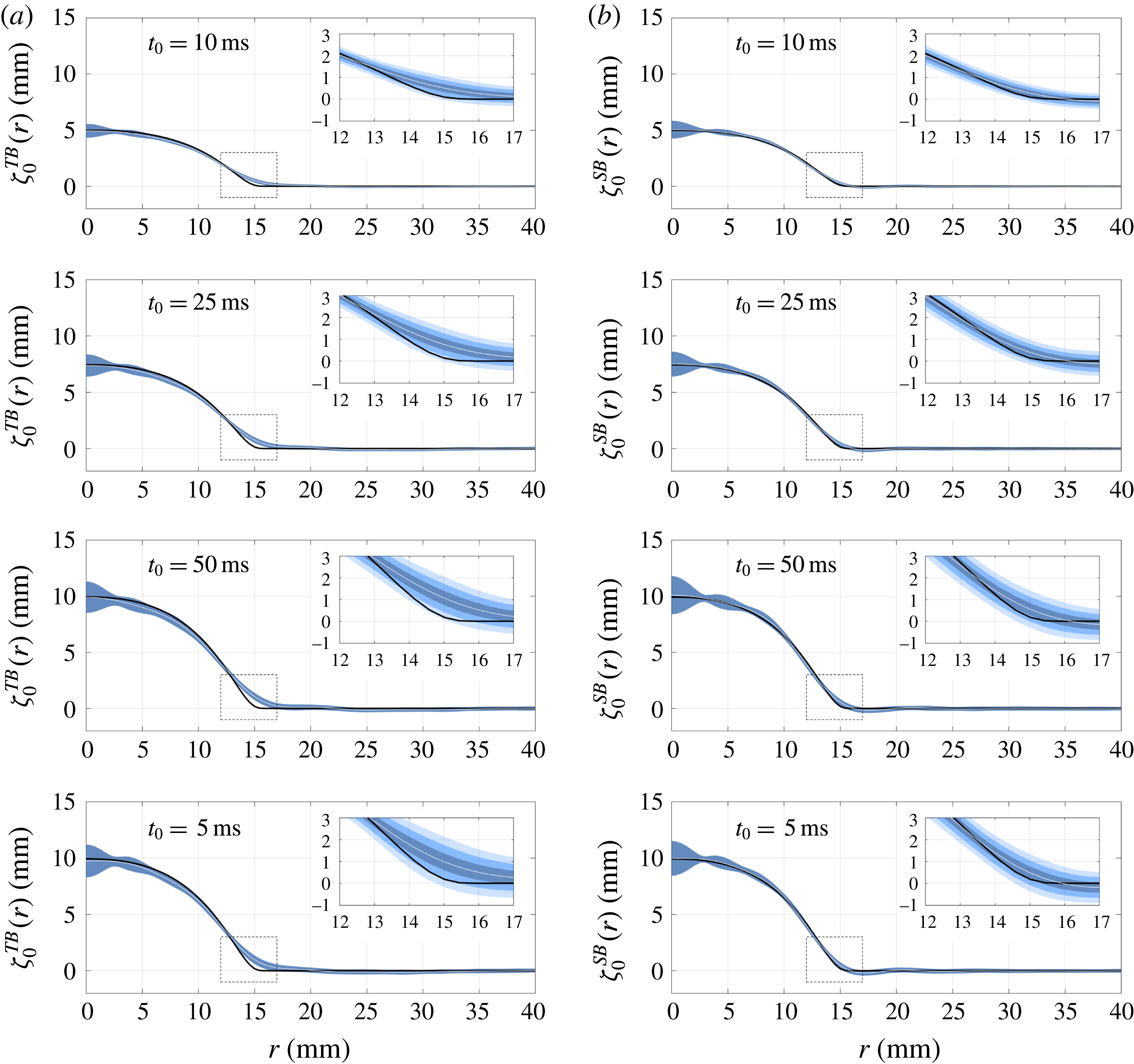
Experimental results for the mean seabed reconstructions for both time- and space-based inversions in four of the 12 cases explored in the present study. Each pair of panels on a given row share the same values of
 $H_{0}$
and
 $t_{0}$
; (a,b) present time- and space-based reconstructions, respectively. The insets show a zoom-in view close to the foot of the bump. White continuous lines denote the mean seabed profiles obtained, while the black curve represents the corresponding imposed seabed deformation. The three shaded regions in the insets correspond to envelopes given by one, two and three times the local standard deviation.
In order to quantify the data dispersion at a particular point on a mean seabed reconstructed profile, we introduce the local (with respect to the
 $r$
variable) standard deviation defined by
 $$\begin{eqnarray}\unicode[STIX]{x1D70E}^{TB}(r)=\sqrt{\langle [\unicode[STIX]{x1D701}_{0}^{TB}(r;r_{\ast })-\langle \unicode[STIX]{x1D701}_{0}^{TB}(r;r_{\ast })\rangle ]^{2}\rangle }\end{eqnarray}$$
for time-based inversions, as well as
 $$\begin{eqnarray}\unicode[STIX]{x1D70E}^{SB}(r)=\sqrt{\langle [\unicode[STIX]{x1D701}_{0}^{SB}(r;t_{\ast })-\langle \unicode[STIX]{x1D701}_{0}^{SB}(r;t_{\ast })\rangle ]^{2}\rangle },\end{eqnarray}$$
which constitutes its equivalent for space-based reconstructions.
Figure 11 illustrates the results obtained for the mean seabed reconstructions for both time- and space-based inversions in four of the 12 cases explored in this work, for radial positions in the range
 $r\leqslant 40~\text{mm}$
. In figure 11, each pair of panels on a given row corresponds to the same values of
 $(H_{0},t_{0})$
; the left and right columns comprise the time- and space-based reconstructions, respectively. In each panel, the mean seabed profile
 $\langle \unicode[STIX]{x1D701}_{0}^{(TB,SB)}(r)\rangle$
is depicted in a white continuous curve, surrounded by a shaded region corresponding to a
 $\pm \unicode[STIX]{x1D70E}^{(TB,SB)}(r)$
envelope. For comparison purposes, the imposed seabed deformation is represented in a black continuous curve. Additionally, each panel contains an inset showing a zoom-in view in the region where the bump meets the flat bottom (enclosed by dashed lines). For radial positions satisfying
 $40~\text{mm}<r\leqslant 178.45~\text{mm}$
, the reconstructions behave similarly to what is observed in the range between 30 and 40 mm, for which reason they are not shown here.
A first remark on figure 11 is that the averaging procedure almost completely removes the oscillations that polluted the individual reconstructions shown in figure 9(a,b), which traduces into a much better agreement between the mean reconstructed profile (white continuous line) and the imposed seabed deformation (black continuous line). Naturally, those oscillations manifest themselves now in the standard deviation envelopes. However, the striking feature here is that those envelopes seem to be modulated by an oscillating amplitude-decreasing function, revealing a spatial coherence between the individual reconstructions that result (through the averaging process) in a mean seabed profile. Moreover, by examining the different panels in figure 11, it is evident that the characteristic length of that modulating function seems to be the same for all cases explored. Even though only four selected cases are shown here, we observed that this last statement is valid for all of our experimental data. We will come back to this point towards the end of this section.
Mean seabed reconstructions for both time- and space-based inversions. The
 $H_{0}$
values are colour coded: red, 5.0 mm; green, 7.5 mm; blue, 10 mm. Symbols refer to different
 $t_{0}$
values: ○,
 $t_{0}=5~\text{ms}$
;
 $\times$
,
 $t_{0}=10~\text{ms}$
; ▫,
 $t_{0}=25~\text{ms}$
;
 $+$
,
 $t_{0}=50~\text{ms}$
. Dash-dotted lines display the imposed seabed deformations as measured by FTP. The inset shows the errors in the reconstructed profiles (respecting the same colour and symbol conventions) as a function of the characteristic time
 $t_{0}$
of the sea-bottom disturbance.

As can be observed by comparing the corresponding figure 11(a,b), the local standard deviations for time- and space-based reconstructions are comparable, i.e.
 $\unicode[STIX]{x1D70E}^{SB}(r)\sim \unicode[STIX]{x1D70E}^{TB}(r)$
for every
 $r$
within a given case. This is indeed expected, in light of the similarities between the results of both types of reconstructions (of which figure 9
a,b are a sample) and the fact that the amount of individual profiles for the averaging process is of the same order for both time- and space-based inversions.
From the first three rows of figure 11, one might think that the maximum values of the local standard deviation increase when the characteristic time of the seabed motion,
 $t_{0}$
, increases, i.e. for slower bottom disturbances. However, this is not the case. Indeed, considering the totality of our results, it is clear there is no correlation between the two quantities. This is evident by comparing the last two rows of panels in figure 11, which correspond to the same value of
 $H_{0}$
(namely, 10 mm) but differ 10-fold in
 $t_{0}$
, yet the local standard deviation shows no appreciable variation.
There remains one last aspect to highlight from the results shown in figure 11, namely the quality of the mean seabed reconstructions near the foot of the bump, which corresponds to the region where the largest differences between reconstructions and the imposed bathymetry take place. In this regard, the insets show that in this zone the mean profiles achieved from space-based inversions agree with the seabed deformation to within 1.5 local standard deviations, whereas those resulting from averaging individual time-based reconstructions tend to deviate further, presenting differences of up to 3 local standard deviations.
Finally, figure 12 sums up our experimental results in terms of the mean seabed reconstructions for all 12 cases considered in this study, organized in two panels according to the type of inversion employed (either time- or space-based). As for the preceding figures, the radial range shown is limited to the region of interest given by
 $r\leqslant 40~\text{mm}$
. In figure 12, each particular value of the maximum bottom deformation height,
 $H_{0}$
, is presented in a different colour and four symbols are used to distinguish the various characteristic times
 $t_{0}$
of the seabed impulsions (see the figure caption for details). For comparison purposes, the imposed seabed deformations (as measured by FTP) are displayed in dash-dotted lines. Moreover, the accompanying insets depict the errors
 $\unicode[STIX]{x1D716}^{(TB,SB)}$
(defined by (5.2a,b
)) and calculated by considering all available realizations) as a function of
 $t_{0}$
. Both the insets and the panels share the same colour and symbol convention to identify corresponding values of the parameter pair
 $(H_{0},t_{0})$
.
These results show that the mean seabed reconstructions are in good agreement with the imposed bottom deformations in all of the explored cases, irrespective of the type of inversion considered. Overall, the associated relative errors, as quantified by
 $\unicode[STIX]{x1D716}^{(TB,SB)}$
, are small: less than 6 % for time-based inversions and below 3 % in the case of space-based reconstructions. Comparatively, space-based inversions follow more closely the shape of the imposed seabed deformations, adequately reproducing the maximum height of the bump as well as its radius. Time-based reconstructions, on the other hand, present larger errors, which arise from a combined underestimation of the former and overshooting of the latter.
The reason for the mean space-based reconstructions outperforming their time-based analogues can be ascribed to two main factors. The first one can be traced back to the condition number of the matrices representing the discrete versions of the functions
 $K(r_{\ast },t,k)$
and
 $K(r,t_{\ast },k)$
in (3.5a
) and (3.5b
), respectively. Calculated as the ratio of the largest to the smallest singular value in the corresponding SVD, the condition number for time-based reconstructions consistently exceeds, by as much as four orders of magnitude, that of the space-based inversions. The second factor involves an intrinsic difference between time and space profiles of the free-surface evolution as stemming from our FTP measurements, and can be explained as follows. In FTP, each measured wave field at a fixed instant is obtained through a process that ultimately involves spatial bandpass filtering of profilometric images (see e.g. Cobelli et al.
Reference Cobelli, Maurel, Pagneux and Petitjeans2009a
), which results in an instantaneous free-surface deformation field,
 $\unicode[STIX]{x1D702}(x,y,t_{\ast })$
, whose high-spatial-frequency noise content is reduced. In contrast, no time-frequency filtering is performed on the whole spatiotemporal set
 $\unicode[STIX]{x1D702}(x,y,t)$
. For this reason, any time series of the local free-surface deformation presents relatively larger high-frequency noise levels than do radial profiles at a given time instant. The combined action of these two independent elements (comparatively better condition number and lower high-frequency noise content) cause space-based inversions to perform better than their time-based equivalents.
In general, we observe a systematic slight reduction in the error with increasing
 $H_{0}$
(evidenced by the consistent colour ordering on the insets, reversed with respect to the panels) and a more pronounced decrease with decreasing
 $t_{0}$
. These two observations suggest that the reconstruction error lessens as the characteristic velocity
 $v$
of the sea-bottom disturbance, estimated as
 $v\sim H_{0}/t_{0}$
, increases. We checked this quantitatively, and obtained a power-law-plus-constant dependence between
 $\unicode[STIX]{x1D716}^{(TB,SB)}$
and
 $v$
with an exponent in the range of
 $-0.81\pm 0.05$
, for both space- and time-based approaches (not shown). This could be attributable to the fact that faster bottom disturbances generate greater deformations at the free surface, which, in turn, redound in spatio-temporal measurements with larger signal-to-noise ratios, leading to better solutions to the inversion problem.
Lastly, let us focus our attention on a point we mentioned briefly in the preceding paragraphs; namely, that regarding the shape of the
 $1\unicode[STIX]{x1D70E}^{(TB,SB)}$
envelopes in figure 11. As we observed previously, and irrespective of reconstruction, those envelopes are modulated by an oscillating amplitude-decreasing function, with null values occurring at the same radial points for all panels and with an almost constant spacing between them.
In order to explain that behaviour, let us consider how a reconstructed seabed profile
 $\unicode[STIX]{x1D701}_{0}(r)$
(be it time- or space-based) is obtained. Through (3.5a
) and (3.5b
), the inversion procedure yields
 $\hat{\unicode[STIX]{x1D701}}_{0}(r)$
, related analytically to the seabed profile by an inverse Hankel transform,
 $$\begin{eqnarray}\unicode[STIX]{x1D701}_{0}(r)=\int _{0}^{\infty }k\text{J}_{0}(kr)\hat{\unicode[STIX]{x1D701}}_{0}(k)\,\text{d}k.\end{eqnarray}$$
In discrete wavenumber form, this expression can be written
 $\unicode[STIX]{x1D701}_{0}(r)=\sum _{i=0}^{\infty }a_{i}\text{J}_{0}(k_{i}r)$
, where
 $a_{i}$
denotes coefficients whose values are independent of the radial variable
 $r$
. Reconstructions obtained from experimental data,
 $\unicode[STIX]{x1D701}_{0}^{\ast }(r)$
, can be decomposed in two additive contributions. One of them involves the experimental noise. The second component is an approximation of
 $\unicode[STIX]{x1D701}_{0}(r)$
to finite order
 $N$
, i.e. a truncation of the original imposed bottom profile given by
 $\unicode[STIX]{x1D701}_{0}^{N}(r)=\sum _{i}^{N}a_{i}\text{J}_{0}(k_{i}r)$
. Therefore, neglecting the effects of experimental noise, the error between the imposed and the reconstructed seabed profiles is
 $\unicode[STIX]{x1D700}=|\unicode[STIX]{x1D701}_{0}(r)-\unicode[STIX]{x1D701}_{0}^{\ast }(r)|=|\sum _{i=N+1}^{\infty }a_{i}\text{J}_{0}(k_{i}r)|$
. This implies that, to leading order, the error satisfies
 $\unicode[STIX]{x1D700}\sim |\text{J}_{0}(k_{N+1}r)|$
, which qualitatively reproduces the spatial characteristics observed in the
 $1\unicode[STIX]{x1D70E}$
envelopes of figure 11. Based on this estimate, the value of
 $k_{N+1}$
can be calculated from the fact that the first minimum of the
 $1\unicode[STIX]{x1D70E}$
envelopes is located at
 $r\simeq 2.5~\text{mm}$
, whereas the first root of the zeroth-order Bessel function of the first kind occurs at approximately 2.4048 (Abramowitz & Stegun Reference Abramowitz and Stegun1964). Hence
 $k_{N+1}\simeq (2.4048/2.5)~\text{rad}~\text{mm}^{-1}\simeq 961~\text{rad}~\text{m}^{-1}$
, which corresponds to a frequency of
 $f_{N+1}\simeq 15~\text{Hz}$
through the dispersion relation for gravity waves (at the working depth). Consistently, a similar value for
 $f_{N+1}$
is obtained by considering the radial position of the second and third minima of the
 $1\unicode[STIX]{x1D70E}$
envelopes and the corresponding roots of the aforementioned Bessel function. Remarkably, this value for
 $f_{N+1}$
can be identified with the maximum frequency for which significant contributions to the experimental energy spectrum are still discernible from the background noise, as discussed in § 4.2. This is consistent with the fact that the quality of the seabed profiles reconstructed by solving the inverse problem based on experimental data is ultimately limited by the information available in the spatiotemporal spectrum of the free-surface deformation, through the upper limits for significant spectral content in frequency–wavenumber space.
6 Summary and conclusions
In this work we studied both theoretically and experimentally the problem of determining the three-dimensional shape of the seabed responsible for the creation of water waves based on an instantaneous global state (space-based inversion) or a local time-history record (time-based inversion) of the free-surface evolution.
In the first part of the paper, we showed that the inversion problem amounts to inverting a Hilbert–Schmidt operator, ill-posed in the sense of Hadamard (Reference Hadamard2003). In order to overcome this difficulty, a Tikhonov regularization scheme was proposed as well as a strategy for choosing the optimal value of the regularization parameter based on the L-curve criterion.
We then conducted a series of laboratory experiments in which an axisymmetric three-dimensional bottom deformation of controlled shape and time evolution was imposed on a layer of water of constant depth, initially at rest. The evolution of the air–water interface was measured by FTP, which provided for both space- and time-resolved data of the free-surface dynamics. By considering the energy spectrum of the free surface, we were able to confirm that the energy is concentrated mainly on a two-dimensional surface in
 $\boldsymbol{k}{-}\unicode[STIX]{x1D714}$
space, defined by the (linear) gravity-wave dispersion relation.
Next, we tested our regularization scheme for obtaining a solution to the inverse problem on our experimental data. Our results show that it is indeed possible to reconstruct the seafloor profile accurately, from either a space- or a time-based inversion. Moreover, our results for the seabed shape exhibit very good agreement with the imposed seabed profiles. We have also shown evidence that it is possible to take advantage of the different reconstructed profiles stemming from various radii (for time-based inversion) or time instants (for space-based inversion) to calculate mean seabed profiles. Moreover, in that case, the error between the imposed bottom deformation and these mean seabed profiles is less than 6 % in the case of time-based reconstructions, and lower than 3 % for space-based inversions. Finally, we show that the content of the spectrum of the free-surface dynamics sets a limit on the accuracy of the reconstructions.
Acknowledgements
A.M., V.P. and P.P. acknowledge support from the Agence Nationale de la Recherche through the grant DYNAMONDE ANR-12-BS09-0027-01. P.J.C. acknowledges support from Chaire Joliot (ESPCI), and grant no. PIP 11220090100825, UBACYT grant no. 20020110200359 and PICT 2011-1529 and 2011-1626, as well as from the Carrera del Investigador Científico of CONICET.



