1 Introduction
The wing hinge position on a flying insect is an inconspicuous feature and is rarely measured. The hinge position relative to the centre of mass is thought to affect flight stability, as indicated by experiments of insects and robotic flyers. For example, a trick to stabilize flapping flight is to add additional surfaces (Fraenkel Reference Fraenkel1939; Childress, Vandenberghe & Zhang Reference Childress, Vandenberghe and Zhang2006; Van Breugel, Regan & Lipson Reference Van Breugel, Regan and Lipson2008; Ristroph et al. Reference Ristroph, Ristroph, Morozova, Bergou, Chang, Guckenheimer, Wang and Cohen2013; Ristroph & Childress Reference Ristroph and Childress2014). These surfaces introduce two effects: an additional aerodynamic drag, which damps the motion, and also a change in the mechanical torque due to the shift between the centre of the mass and the centre of pressure. It is difficult to separate these two effects in experiments.
To understand the effect of the wing hinge position on flight stability, we carry out a computational analysis of flight stability. We find that both hovering and ascending flights are unstable, and that stability has a weak dependence on the hinge position. The hinge position however affects the ascending speed of flight. We find that there is an optimal hinge position, at which the periodic flight solution attains the maximal ascending speed, for a given stroke amplitude. Interestingly, this optimal hinge position is independent of the stroke amplitude. We note that at the optimal hinge location, the body oscillation due to flapping wing motion is minimized, resembling an anti-resonance. To find a minimal model that captures the dynamic coupling between the wings and the body, we analysed a simplified model of two coupled masses. The model predicts the dependence of the optimal location on the morphological parameters. For the model fly, the optimal hinge position is approximately half-way between the centre of mass and the top of the body.
These analyses are a part of an ongoing search for optimal solutions in animal locomotion (Alexander Reference Alexander2001; Srinivasan & Ruina Reference Srinivasan and Ruina2006; Berman & Wang Reference Berman and Wang2007; Alben Reference Alben2008; Pesavento & Wang Reference Pesavento and Wang2009; Wang Reference Wang2016). Optimality in natural systems is often difficult to quantify, as we do not know a priori which functions the animals optimize, if any at all. Each organism has a large number of parameters at their disposal, and is likely to improve multiple traits simultaneously in the course of evolution. These unknowns make the study of optimality a seemingly intractable problem (Gould & Lewontin Reference Gould and Lewontin1979). On the other hand, there is evidence that animal behaviour often pushes the physical limits (Bialek Reference Bialek1987; Haselsteiner, Gilbert & Wang Reference Haselsteiner, Gilbert and Wang2014). One way to make progress is to make quantitative predictions to test optimality of specific traits, and we hope the predicted
 $h^{\ast }$
will be tested by experiments.
2 Methods
In order to study the stability of insect flight we use a three-dimensional dynamical flight simulation, which determines the time evolution of a flight for prescribed wing motions. The flight simulation was described in Chang & Wang (Reference Chang and Wang2014) and is summarized below. The new element in our analysis is the search for periodic orbits and their stability using Floquet analysis (Grimshaw Reference Grimshaw1991; Kuznetsov Reference Kuznetsov2013; Iams & Guckenheimer Reference Iams and Guckenheimer2014; Sun Reference Sun2014). To find periodic orbits we search numerically for initial flight states that return to themselves after a wing beat. The stability of these periodic solutions is given by the eigenvalues of the linearized Poincare map for this periodic initial state.
2.1 Three-dimensional dynamic flight simulation
To simulate three-dimensional free flight with flapping wings, we solve the Newton–Euler equations for the coupled wing–body system (Chang & Wang Reference Chang and Wang2014). The insect model consists of
 $(n+1)$
rigid bodies, where
 $n$
is the number of wings on the body. Each wing is modelled as an ellipsoid connected to the body, also an ellipsoid, through a ball joint that allows for three degrees of freedom in rotation. The body kinematics are given by its position
 $\boldsymbol{r}^{b}$
, linear velocity
 $\boldsymbol{v}^{b}$
, body orientation quaternion
 $[q^{b}]$
and angular velocity
 $\unicode[STIX]{x1D74E}^{b}$
. In our current implementation we use quaternions to represent the body and wing orientations. This has the advantage of avoiding gimbal lock and simplifies the algebra. For the results the quaternions are converted to Euler angles, which are easier to understand, as they refer to the rotations about body axes.
The Newton–Euler equations governing the body dynamics are
 $$\begin{eqnarray}\displaystyle & \displaystyle m^{b}\boldsymbol{a}^{b}=m^{b}\boldsymbol{g}-\mathop{\sum }_{i=1}^{n}\boldsymbol{F}_{i}^{c}, & \displaystyle\end{eqnarray}$$
 $$\begin{eqnarray}\displaystyle & \displaystyle \unicode[STIX]{x1D644}^{b}\unicode[STIX]{x1D737}^{b}=-\unicode[STIX]{x1D74E}^{b}\times (\unicode[STIX]{x1D644}^{b}\unicode[STIX]{x1D74E}^{b})-\mathop{\sum }_{i=1}^{n}\unicode[STIX]{x1D749}_{i}^{c}-\mathop{\sum }_{i=1}^{n}\boldsymbol{r}_{i}^{b}\times \unicode[STIX]{x1D749}_{i}^{c}. & \displaystyle\end{eqnarray}$$
Similarly, the governing equations for the
 $i$
th wing are
 $$\begin{eqnarray}\displaystyle & \displaystyle m_{i}^{w}\boldsymbol{a}_{i}^{w}=m_{i}^{w}\boldsymbol{g}+\boldsymbol{F}_{i}^{c}+\boldsymbol{F}_{i}^{a}, & \displaystyle\end{eqnarray}$$
 $$\begin{eqnarray}\displaystyle & \displaystyle \unicode[STIX]{x1D644}_{i}^{w}\unicode[STIX]{x1D737}_{i}^{w}=-\unicode[STIX]{x1D74E}_{i}^{w}\times (\unicode[STIX]{x1D644}_{i}^{w}\unicode[STIX]{x1D74E}_{i}^{w})+\unicode[STIX]{x1D749}_{i}^{c}+\boldsymbol{r}_{i}^{w}\times \unicode[STIX]{x1D749}_{i}^{c}+\unicode[STIX]{x1D749}_{i}^{a}. & \displaystyle\end{eqnarray}$$
Here
 $b$
denotes body,
 $w$
denotes wing,
 $m$
is mass,
 $\unicode[STIX]{x1D644}$
is the moment of inertia tensor,
 $\boldsymbol{a}$
is the linear acceleration,
 $\unicode[STIX]{x1D737}$
is the angular acceleration,
 $\boldsymbol{g}$
is the gravitational constant,
 $\unicode[STIX]{x1D74E}$
is the angular velocity,
 $\boldsymbol{F}^{a}$
and
 $\unicode[STIX]{x1D749}^{a}$
are the aerodynamic force and torque on the wing,
 $\boldsymbol{F}_{i}^{c}$
and
 $\unicode[STIX]{x1D749}_{i}^{c}$
are the internal force and torque to be determined,
 $\boldsymbol{r}_{i}^{b}$
is the position of the
 $i$
th wing root relative to the body centre of mass (COM) and
 $\boldsymbol{r}_{i}^{w}$
is the position of the
 $i$
th wing root relative to the COM of the
 $i$
th wing.
Because we have introduced unknown variables in the form of the internal forces and torques at the joint,
 $\boldsymbol{F}^{c}$
and
 $\unicode[STIX]{x1D749}^{c}$
, additional equations must be specified. These equations are two kinematic constraints applied at each wing joint. The first is on the angular acceleration of the wing relative to the body,
 $$\begin{eqnarray}\unicode[STIX]{x1D737}_{i}^{r}=\unicode[STIX]{x1D737}_{i}^{w}-\unicode[STIX]{x1D737}^{b},\end{eqnarray}$$
which states that the wing acceleration relative to the body must be the prescribed acceleration. The second constraint is the matching condition for the linear acceleration of the wing hinge:
 $$\begin{eqnarray}\boldsymbol{a}^{b}+\unicode[STIX]{x1D737}^{b}\times \boldsymbol{r}_{i}^{b}+\unicode[STIX]{x1D74E}^{b}\times (\unicode[STIX]{x1D74E}^{b}\times \boldsymbol{r}_{i}^{b})=\boldsymbol{a}^{w}+\unicode[STIX]{x1D737}^{w}\times \boldsymbol{r}_{i}^{w}+\unicode[STIX]{x1D74E}^{w}\times (\unicode[STIX]{x1D74E}^{w}\times \boldsymbol{r}_{i}^{w}).\end{eqnarray}$$
At each instance in time, the coupled dynamic equations (2.1)–(2.4) together with the constraint equations (2.5) and (2.6) can be cast into a linear system,
 $\text{A}x=\text{B}$
, where
 $x=[\boldsymbol{a}^{b},\unicode[STIX]{x1D737}^{b},\boldsymbol{a}_{i}^{w},\unicode[STIX]{x1D737}_{i}^{w},\boldsymbol{F}_{i}^{c},\unicode[STIX]{x1D749}_{i}^{c}]$
, and
 $\text{A}$
contains
 $m_{i}$
and
 $\unicode[STIX]{x1D644}_{i}$
, and the vector
 $\text{B}$
contains the known variables with
 $\unicode[STIX]{x1D74E}_{i}$
,
 $\boldsymbol{F}_{i}^{a}$
and
 $\unicode[STIX]{x1D749}_{i}^{a}$
evaluated at the current time. We solve this system of equations by inverting the matrix
 $\text{A}$
, using standard lower–upper (LU) decomposition, to find the body accelerations.
Once the body accelerations
 $\boldsymbol{a}^{b}$
and
 $\unicode[STIX]{x1D737}^{b}$
are obtained, the body kinematic state evolves in time according to
 $$\begin{eqnarray}\displaystyle & \displaystyle \dot{\boldsymbol{r}}^{b}=[q]^{b}(\boldsymbol{v}^{b}), & \displaystyle\end{eqnarray}$$
 $$\begin{eqnarray}\displaystyle & \displaystyle \dot{\boldsymbol{v}}^{b}=\boldsymbol{a}^{b}-\unicode[STIX]{x1D74E}^{b}\times \boldsymbol{v}^{b}, & \displaystyle\end{eqnarray}$$
 $$\begin{eqnarray}\displaystyle & \displaystyle [\dot{q}]^{b}={\textstyle \frac{1}{2}}[q]^{b}\cdot [\unicode[STIX]{x1D714}]^{b}, & \displaystyle\end{eqnarray}$$
 $$\begin{eqnarray}\displaystyle & \displaystyle \dot{\unicode[STIX]{x1D74E}}^{b}=\unicode[STIX]{x1D737}^{b}. & \displaystyle\end{eqnarray}$$
Here equation (2.7) rotates the velocity vector from the body frame to the laboratory frame. This quaternion rotation of a vector can be written out in normal vector products by separating the real part,
 $q_{0}$
, and complex part,
 $\boldsymbol{q}$
, of the quaternion as
 $[q]=(q_{0},\boldsymbol{q})$
. Equation (2.7) becomes
 $$\begin{eqnarray}\dot{\boldsymbol{r}}^{b}=\boldsymbol{v}^{b}+2\boldsymbol{q}^{b}\times (\boldsymbol{q}^{b}\times \boldsymbol{v}^{b}+q_{0}^{b}\boldsymbol{v}^{b}).\end{eqnarray}$$
In (2.9) the operator is quaternion multiplication, which is possible after promoting
 $[\unicode[STIX]{x1D714}]^{b}$
to a quaternion by adding a zero real part, i.e.
 $[\unicode[STIX]{x1D714}]^{b}=(0,\unicode[STIX]{x1D74E}^{b})$
. This set of nonlinear ordinary differential equations is solved using an adaptive order Adams–Bashforth–Moulton algorithm that ensures the quaternion
 $[q]^{b}$
remains unitary and thus a representation of the body orientation (Shampine & Gordon Reference Shampine and Gordon1975).
2.1.1 Aerodynamic force model on the wing
The dynamic equations, (2.1)–(2.4), require the specification of the aerodynamic force and torque on the wings. Our force model is a quasi-steady force approximation that takes into account the main unsteady effects, including the dynamic stall, the coupling between wing translation and rotation and the added mass term (Wang Reference Wang2005). The forces on the wings are decomposed into three parts, corresponding to the lift, the drag and the added mass, i.e.
 $\boldsymbol{F}_{i}^{a}=\boldsymbol{F}_{L}+\boldsymbol{F}_{D}+\boldsymbol{F}_{A}$
. We use the blade element approximation and divide the wing into infinitesimal wing blades,
 $\boldsymbol{F}=\int \boldsymbol{f}(s)\,\text{d}s$
and
 $\unicode[STIX]{x1D749}=\int \boldsymbol{s}\times \boldsymbol{f}(s)\,\text{d}s$
, with
 $s$
the coordinate along the span.
The specific form of the lift and drag on each blade element is deduced from experiments and numerical simulations of a free falling plate in fluid (Pesavento & Wang Reference Pesavento and Wang2004; Andersen, Pesavento & Wang Reference Andersen, Pesavento and Wang2005). The lift force density is given by
 $\boldsymbol{f}_{L}(s)=-\unicode[STIX]{x1D70C}_{f}\unicode[STIX]{x1D71E}(s)\times \boldsymbol{v}(s)$
, with the circulation
 $\unicode[STIX]{x1D71E}(s)=(c(s)/2)[C_{T}(\unicode[STIX]{x1D6FC})v(s)\sin (2\unicode[STIX]{x1D6FC}(s))-C_{R}(\unicode[STIX]{x1D6FC})c(s)\unicode[STIX]{x1D714}_{x}]\hat{\boldsymbol{s}}$
. Here
 $\hat{\boldsymbol{s}}$
is the outward unit vector along the span,
 $\unicode[STIX]{x1D70C}_{f}$
is the fluid density,
 $C_{T}$
and
 $C_{R}$
are force coefficients that depend on
 $\unicode[STIX]{x1D6FC}$
,
 $c(s)$
is the local chord length,
 $\unicode[STIX]{x1D714}_{x}$
is the
 $x$
-component of the angular velocity and
 $v(s)$
is the magnitude of the local wing velocity.
 $\unicode[STIX]{x1D6FC}$
denotes the angle of attack, which is the angle between the wing chord and the velocity vector. The damping force density is given by:
 $\boldsymbol{f}_{D}=-\unicode[STIX]{x1D70C}_{f}k(s)\boldsymbol{v}(s)$
, with
 $k(s)=(1/2)c(s)v(s)(\text{A}-\text{B}\cos (2\unicode[STIX]{x1D6FC}(s)))$
and
 $\text{A}$
and
 $\text{B}$
are constants. The aerodynamic force parameters are fixed at
 $C_{T}=1.5$
,
 $C_{R}=\unicode[STIX]{x03C0}$
,
 $\text{A}=1.4$
,
 $\text{B}=1$
and
 $\unicode[STIX]{x1D70C}_{f}=1.293~\text{kg}~\text{m}^{-3}$
.
The added mass term represents the force needed to accelerate the wing in a potential flow. For ellipsoids, the added mass and torque have exact expressions:
 $$\begin{eqnarray}\displaystyle & \displaystyle \boldsymbol{F}_{added}=\left(\begin{array}{@{}c@{}}-m_{33}v_{z}\unicode[STIX]{x1D714}_{y}\\ m_{33}v_{z}\unicode[STIX]{x1D714}_{x}\\ -m_{33}\dot{v}_{z}\end{array}\right), & \displaystyle\end{eqnarray}$$
 $$\begin{eqnarray}\displaystyle & \displaystyle \unicode[STIX]{x1D749}_{added}=\left(\begin{array}{@{}c@{}}-m_{44}\dot{\unicode[STIX]{x1D714}}_{x}+m_{55}\unicode[STIX]{x1D714}_{y}\unicode[STIX]{x1D714}_{z}-m_{33}v_{y}v_{z}\\ -m_{55}\dot{\unicode[STIX]{x1D714}}_{y}-m_{44}\unicode[STIX]{x1D714}_{x}\unicode[STIX]{x1D714}_{z}+m_{33}v_{x}v_{z}\\ (m_{44}-m_{55})\unicode[STIX]{x1D714}_{x}\unicode[STIX]{x1D714}_{y}\end{array}\right). & \displaystyle\end{eqnarray}$$
Here
 $v$
and
 $\unicode[STIX]{x1D714}$
are the velocity and angular velocity at the centre of mass of the wing. The added mass coefficients,
 $m_{33}$
,
 $m_{44}$
and
 $m_{55}$
, are (Tuckerman Reference Tuckerman1926)
 $$\begin{eqnarray}\displaystyle & \displaystyle m_{33}=\frac{4}{3}\unicode[STIX]{x03C0}\unicode[STIX]{x1D70C}_{f}\frac{ab^{2}}{E(k)}, & \displaystyle\end{eqnarray}$$
 $$\begin{eqnarray}\displaystyle & \displaystyle m_{44}=\frac{4}{15}\unicode[STIX]{x03C0}\unicode[STIX]{x1D70C}_{f}ab^{4}\frac{a^{2}-b^{2}}{(2a^{2}-b^{2})E(k)-b^{2}K(k)}, & \displaystyle\end{eqnarray}$$
 $$\begin{eqnarray}\displaystyle & \displaystyle m_{55}=\frac{4}{15}\unicode[STIX]{x03C0}\unicode[STIX]{x1D70C}_{f}a^{3}b^{2}\frac{a^{2}-b^{2}}{(a^{2}-2b^{2})E(k)+b^{2}K(k)}, & \displaystyle\end{eqnarray}$$
with
 $K(k)$
and
 $E(k)$
the elliptic integrals of the first and second kind respectively.
 $k=1-(b/a)^{2}$
, with
 $a$
the semi-major axis, half-span, and
 $b$
the semi-minor axis, half-chord.
2.2 Wing motion
The wings flap back and forth along a horizontal stroke plane following a pattern similar to that observed in flies. We use a generalized family of wing motions for the three wing angles:
 $\unicode[STIX]{x1D719}^{w}(t)$
, the stroke angle,
 $\unicode[STIX]{x1D703}^{w}(t)$
, the deviation angle and
 $\unicode[STIX]{x1D713}^{w}(t)$
, the wing-pitch angle (Berman & Wang Reference Berman and Wang2007),
 $$\begin{eqnarray}\displaystyle & \displaystyle \unicode[STIX]{x1D719}^{w}(t)=\unicode[STIX]{x1D719}_{0}+\unicode[STIX]{x1D719}_{m}\frac{\arcsin (K\sin (2\unicode[STIX]{x03C0}ft))}{\arcsin (K)}, & \displaystyle\end{eqnarray}$$
 $$\begin{eqnarray}\displaystyle & \displaystyle \unicode[STIX]{x1D703}^{w}(t)=\unicode[STIX]{x1D703}_{0}+\unicode[STIX]{x1D703}_{m}\cos (N\cdot 2\unicode[STIX]{x03C0}ft+\unicode[STIX]{x1D6FF}_{\unicode[STIX]{x1D703}}), & \displaystyle\end{eqnarray}$$
 $$\begin{eqnarray}\displaystyle & \displaystyle \unicode[STIX]{x1D713}^{w}(t)=\unicode[STIX]{x1D713}_{0}+\unicode[STIX]{x1D713}_{m}\frac{\tanh (C\sin (2\unicode[STIX]{x03C0}ft+\unicode[STIX]{x1D6FF}_{\unicode[STIX]{x1D713}}))}{\tanh (C)}, & \displaystyle\end{eqnarray}$$
where
 $\unicode[STIX]{x1D719}_{0}$
,
 $\unicode[STIX]{x1D703}_{0}$
and
 $\unicode[STIX]{x1D713}_{0}$
set the mean;
 $\unicode[STIX]{x1D719}_{m}$
,
 $\unicode[STIX]{x1D703}_{m}$
and
 $\unicode[STIX]{x1D713}_{m}$
are amplitudes;
 $f$
is the wing-beat frequency;
 $\unicode[STIX]{x1D6FF}_{\unicode[STIX]{x1D703}}$
and
 $\unicode[STIX]{x1D6FF}_{\unicode[STIX]{x1D713}}$
are phase shifts;
 $N=1$
or
 $2$
,
 $0<K<1$
and
 $C>0$
are waveform control parameters.
 $N=1$
corresponds to one vertical oscillation per stroke, and
 $N=2$
corresponds to a figure-eight motion.
 $\unicode[STIX]{x1D719}^{w}$
becomes sinusoidal when
 $K$
is close to
 $0$
and triangular when
 $K$
is close to
 $1$
.
 $\unicode[STIX]{x1D713}^{w}$
becomes sinusoidal at small
 $C$
and a step function at large
 $C$
. For simplicity, the deviation
 $\unicode[STIX]{x1D703}$
from the main stroke plane is neglected, and the phase shift
 $\unicode[STIX]{x1D6FF}_{\unicode[STIX]{x1D713}}$
in
 $\unicode[STIX]{x1D713}^{w}(t)$
is such that the wing pitches in advance of the wing stroke reversal. For the calculations reported here, the base parameters are
 $f=250~\text{Hz}$
,
 $\unicode[STIX]{x1D719}_{m}=70^{\circ }$
,
 $\unicode[STIX]{x1D719}_{0}=0^{\circ }$
,
 $K=0.7$
,
 $\unicode[STIX]{x1D703}_{m}=\unicode[STIX]{x1D703}_{0}=0^{\circ }$
,
 $\unicode[STIX]{x1D713}_{m}=53^{\circ }$
,
 $\unicode[STIX]{x1D713}_{0}=90^{\circ }$
,
 $\unicode[STIX]{x1D6FF}_{\unicode[STIX]{x1D713}}=72.4^{\circ }$
and
 $C=2.4$
(Berman & Wang Reference Berman and Wang2007; Chang & Wang Reference Chang and Wang2014). When a parameter is varied in the study, it is stated in the relevant figure.
2.3 Morphological parameters
For comparison with related studies we use morphological parameters similar to those of fruit flies, Drosophila melanogaster, we start with the same set of parameters as in (Chang & Wang Reference Chang and Wang2014): body mass
 $m_{b}=1.1~\text{mg}$
, length
 $=2.4~\text{mm}$
, width
 $=1.2~\text{mm}$
; wing mass
 $m_{w}=3.6\times 10^{-3}~\text{mg}$
, span
 $=2~\text{mm}$
, maximal chord
 $=1~\text{mm}$
and maximal thickness
 $=0.1~\text{mm}$
. The wings are attached
 $h=1~\text{mm}$
vertically up from and
 $0.36~\text{mm}$
to the side of the body centre of mass (COM), with the COM of the wing
 $s_{x}=0.87~\text{mm}$
along the span and
 $s_{y}=0.25~\text{mm}$
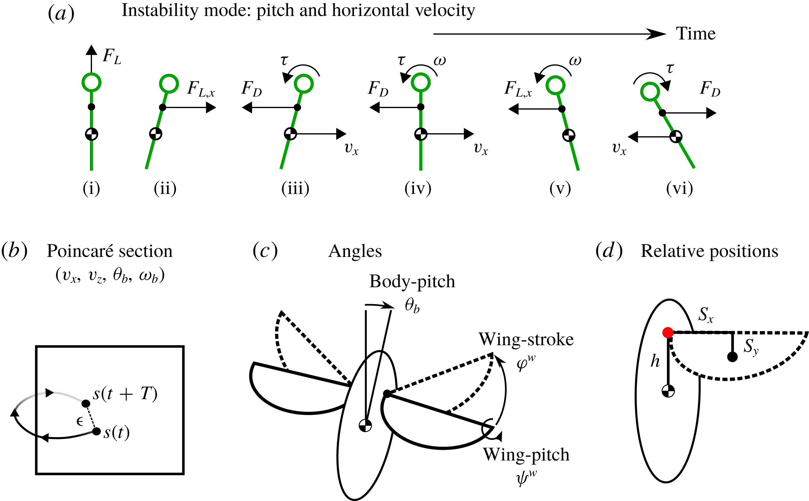
along the chord direction from the hinge location (see figure 1
d). When a parameter is varied, it is stated in the relevant figure. For theoretical interest, the hinge position is chosen to be in the range of
 $h\in [-2,8]~\text{mm}$
, which corresponds to 1 body length below and 4 body lengths above the centre of mass of the fly.
(a) The main mode of flight stability is the pitch instability, and it is due to the coupling between the forward motion and the body pitching motion. The stick shows the body pitch axis, with the circle indicating the top of the body. In both hovering and ascending flight, the body oscillation grows and the flight becomes unstable. Only in descending flight can an upward drag force stabilize the oscillation. (b) The Poincaré section for longitudinal flight. The state variables are
 $(v_{x},v_{y},\unicode[STIX]{x1D703},\unicode[STIX]{x1D714})$
. The flight model maps the initial state
 $s(t)$
to
 $s(t+T)$
after one wing beat. Periodic flight corresponds to fixed points of this map. (c) The wing motion has two degrees of freedom, the back and forth stroke
 $\unicode[STIX]{x1D719}^{w}$
, and the rotation about the pitching axis, the wing pitch
 $\unicode[STIX]{x1D713}^{w}$
. Left and right symmetry ensures that the body moves along the longitudinal plane. The tilt of the body away from the vertical is
 $\unicode[STIX]{x1D703}_{b}$
. (d) Morphological parameters.
 $h$
denotes the wing hinge position (red dot above the body centre of mass (COM)).
 $s_{x}$
and
 $s_{y}$
define the location of the wing COM relative to the hinge.

2.4 Periodic orbit search and stability computation
The stability of periodic flights are analysed using Floquet analysis. For this, we first need to identify periodic flight states (figure 1
b). The left and right wings flap symmetrically leading to longitudinal flights. The state vector is four-dimensional,
 $\boldsymbol{s}=[v_{x},v_{z},\unicode[STIX]{x1D703}_{b},\unicode[STIX]{x1D714}_{y}]$
, where
 $v_{x}$
and
 $v_{z}$
are the horizontal and vertical velocities, and
 $\unicode[STIX]{x1D703}_{b}$
and
 $\unicode[STIX]{x1D714}_{y}$
are the body pitch angle and the pitching rate. A periodic state is found by adjusting the initial state
 $\boldsymbol{s}_{0}$
until it minimizes the periodicity error
 $\unicode[STIX]{x1D716}=\Vert M(\boldsymbol{s}_{0})-\boldsymbol{s}_{0}\Vert$
, using root-finding algorithms. Here
 $M$
represents the evolution of flight dynamics,
 $\boldsymbol{s}(t+T)=M(\boldsymbol{s}(t)),$
with
 $T$
the wing-beat period. The search algorithm consists of successive minimal searches, with each cycle combining the previous best periodic state with periodic states of nearby model parameters to seed a new minimum search.
The function
 $M$
defines a Poincaré map on our flight state space. The periodic flight states correspond to fixed points of this map. We also investigated whether other periodic orbits exist, by starting from very different initial conditions and looking for period-2 orbits. All results converge to the same periodic states as reported here, suggesting a unique solution.
The stability of flight is given by the eigenvalues of the Jacobian of
 $M$
. The eigenvalues of the Jacobian matrix
 $\unicode[STIX]{x1D63F}$
measure the growth rate of the deviation from periodic flight (Grimshaw Reference Grimshaw1991; Kuznetsov Reference Kuznetsov2013). To find these eigenvalues we first compute
 $\unicode[STIX]{x1D63F}$
,
 $$\begin{eqnarray}\unicode[STIX]{x1D63F}=\left.\frac{\unicode[STIX]{x2202}}{\unicode[STIX]{x2202}\boldsymbol{s}}\left(\frac{M(T,\boldsymbol{s})-\boldsymbol{s}}{T}\right)\right|_{s=s_{0}}.\end{eqnarray}$$
The eigenvalues
 $\unicode[STIX]{x1D706}$
of
 $\unicode[STIX]{x1D63F}$
are known as the Lyapunov exponents. If
 $\max (\text{Re}(\unicode[STIX]{x1D706}))<0$
the deviations decrease over time and the periodic flight is stable. Moreover, the eigenvectors of
 $\unicode[STIX]{x1D63F}$
will indicate which deviations lead to instability.
For ease of interpretation, we define
 $\unicode[STIX]{x1D6FC}=\exp (\unicode[STIX]{x1D706}T)$
, which is the multiplicative factor by which a deviation grows after a single wing beat. These
 $\unicode[STIX]{x1D6FC}$
values are called the multipliers of the Poincaré map associated with our model
 $M$
. If all
 $|\unicode[STIX]{x1D6FC}_{i}|<1$
, then the deviations decay and the flight is stable. However, if there is at least one
 $|\unicode[STIX]{x1D6FC}_{i}|>1$
then the flight is unstable.
3 Results
3.1 Hovering and ascending flights are unstable irrespective of the hinge position
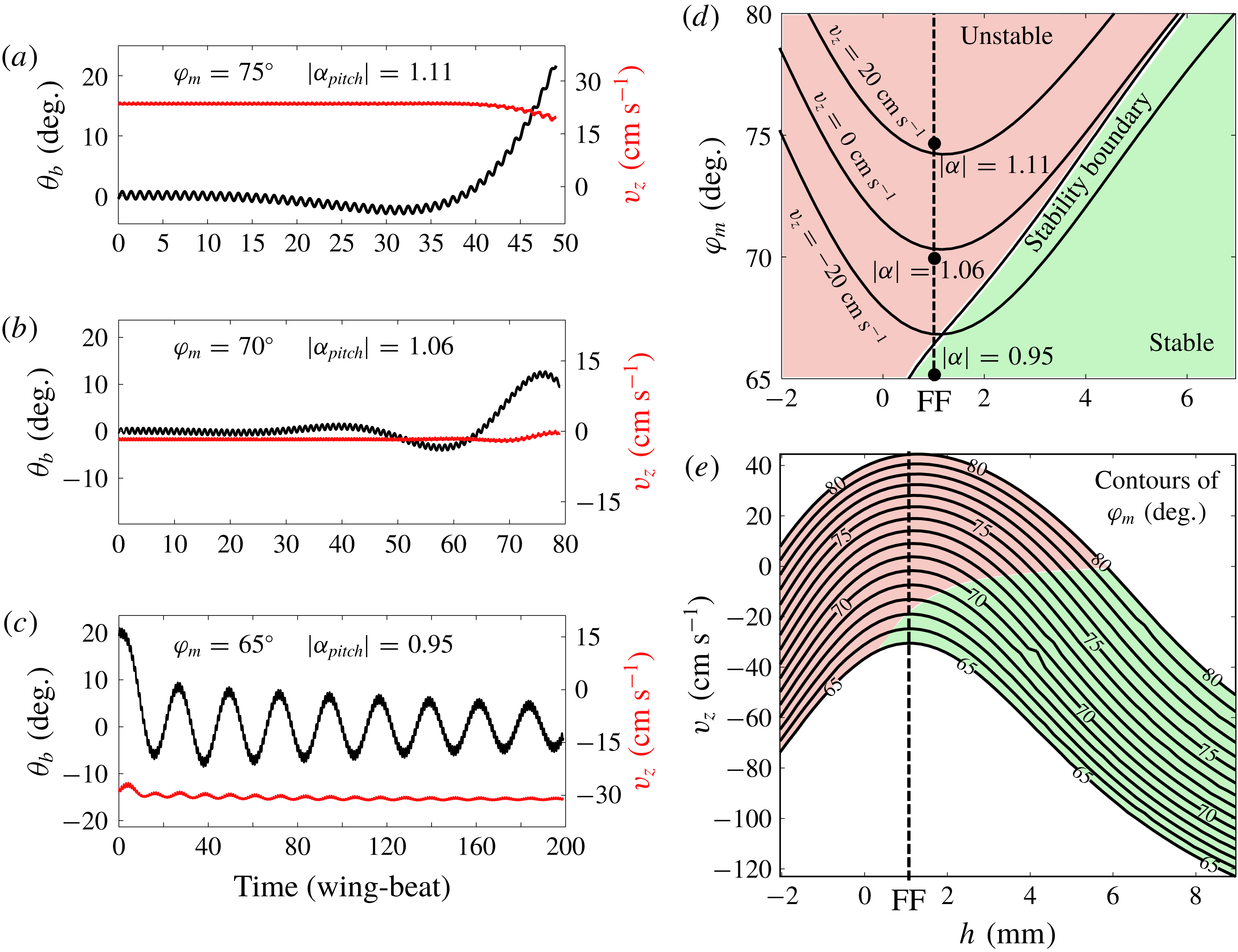
Using the Floquet analysis of periodic flight states, we calculated the stability of flight at different vertical speeds, by varying the stroke amplitude and the hinge position. Figure 2(d) shows that both hovering and ascending flight are unstable. Interestingly, raising the hinge position does not change the stability of hovering and ascending flight. Figure 2(a) shows an unstable ascending flight, with
 $\max (|\unicode[STIX]{x1D6FC}_{i}|)=1.11$
. With an initial deviation of
 $0.1^{\circ }$
in
 $\unicode[STIX]{x1D703}_{b}$
, the pitch continues to drift, and after approximately 30 wing beats, the fly tumbles. Figure 2(b) shows an unstable hovering flight, with
 $\max (|\unicode[STIX]{x1D6FC}_{i}|)=1.06$
. Figure 2(c) shows a stable descending flight, with
 $\max (|\unicode[STIX]{x1D6FC}_{i}|)=0.95$
, in which the a large initial deviation of
 $20^{\circ }$
decays.
(a–c) Stability of ascending, hovering and descending flight. (a,b) Start with a small pitch deviation of
 $\unicode[STIX]{x1D703}_{b}\sim 0.1^{\circ }$
away from periodic flight, and the deviation grows. (c) Starts with a pitch deviation of
 $20^{\circ }$
, and the deviation decays. (d) Contour plot showing how the vertical velocity depends on stroke amplitude and hinge location. The stability boundary corresponds to the line defined by
 $|\unicode[STIX]{x1D6FC}|=1$
. The dashed line corresponds to model fly’s nominal hinge position, half-way between the centre of mass and the top of the body. Black dots correspond to the example flights shown in (a–c). (e) Vertical velocity as a function of the stroke amplitude. The maximum velocity occurs at
 $h=1$
, independent of the stroke amplitude. Each contour is for a constant stroke amplitude. Colour indicates stability, following the same scheme as in part (d).

The main mode of instability for a longitudinal flight is the pitch instability (Sun, Wang & Xiong Reference Sun, Wang and Xiong2007; Cheng & Deng Reference Cheng and Deng2011; Ma et al.
Reference Ma, Chirarattananon, Fuller and Wood2013; Ristroph et al.
Reference Ristroph, Ristroph, Morozova, Bergou, Chang, Guckenheimer, Wang and Cohen2013; Chang & Wang Reference Chang and Wang2014; Sun Reference Sun2014), due to the dynamic coupling between the body pitch and forward motion (figure 1
a). This instability is due to the coupling between the pitching and horizontal motion. An initial deviation in pitch directs the lift force forward, which results in a horizontal velocity. This horizontal velocity adds a bias to the wing motion and produces a net drag. Because that the centre of pressure is not at the centre of mass, the drag torque pitches the body. This coupling between the translational velocity and the body pitch motion leads to the pitch instability (figure 2
a). The calculations here further show that both hovering and ascending flight are unstable, regardless of the hinge position. Hovering flight is close to the stability boundary and the instability increases with the ascending speed. The fruit fly’s nominal hinge location
 $h=1~\text{mm}$
does not appear to have special stability properties (figure 2
d, dashed line).
3.2 Optimal hinge position
Unexpectedly, there is a special hinge position at
 $h_{0}=1~\text{mm}$
that maximizes the ascending speed. Moreover, this optimal hinge position is independent of the stroke amplitude (figure 2
e). The remainder of this paper explains why this is so.
3.2.1 Anti-resonance
The existence of an optimal
 $h$
has to do with the dynamics of body–wing coupling. This coupling can be viewed as an inverted pendulum driven by a pair of oscillating forces. As the body oscillates, the wing hinge acquires an additional velocity,
 $v_{h}=\unicode[STIX]{x1D714}_{y}h$
. Since the body moves in the opposite direction to the wing, such a coupling reduces the effective wing velocity relative to the air,
 $v_{w}$
, and thereby the aerodynamic forces. Moreover, the body oscillation directs the lift away from vertical. When the body oscillation is minimized, the upward force is maximized, and so is the ascending speed.
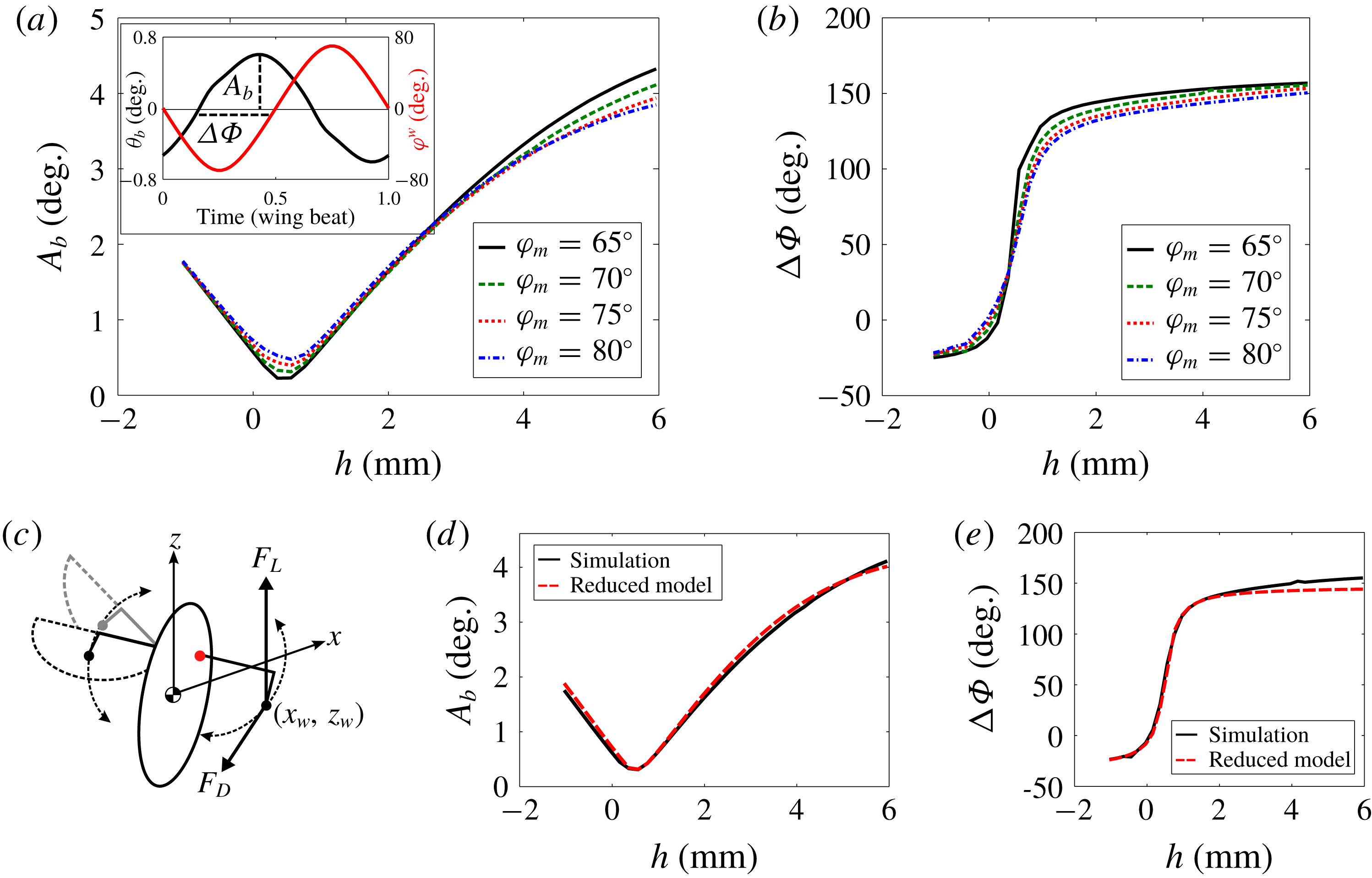
(a) Amplitude of the body oscillation as a function of
 $h$
. The minimal amplitude occurs at
 $h=0.5~\text{mm}$
, irrespective of the stroke amplitude. The inset shows that the body oscillation
 $\unicode[STIX]{x1D703}_{b}$
is approximately a linear response to the wing stroke
 $\unicode[STIX]{x1D719}^{w}$
. This allows us to define the amplitude
 $A_{b}$
and the phase shift
 $\unicode[STIX]{x0394}\unicode[STIX]{x1D6F7}$
. (b) The phase shift as a function of
 $h$
. There is a jump of
 $180^{\circ }$
around
 $h=0.5~\text{mm}$
, independent of the stroke amplitude. These graphs suggest that the hinge position can be tuned into an anti-resonance in the body pitch response. (c) The simplified model considers the wings as point masses at the original COM (black dots). The point mass move along an arc in a sinusoidal motion, and experience a constant lift,
 $F_{L}$
and drag,
 $F_{D}$
. (d,e) The simplified model captures the anti-resonance seen in the simulations.

Figure 3(a,b) shows the amplitude of the body oscillation,
 $A_{b}$
, and the phase delay between the body pitch and wing motion,
 $\unicode[STIX]{x0394}\unicode[STIX]{x1D6F7}$
, as a function of
 $h$
. The body oscillation is minimized at
 $h^{\ast }=0.5~\text{mm}$
accompanied by a phase jump. These are signatures of an anti-resonance.
3.2.2 A reduced model for analysing the anti-resonance
To understand why the optimal
 $h$
is independent of the stroke amplitude, we construct a simplified dynamic model, which consists of two point masses that experience lift and drag forces. The model exhibits an anti-resonance similar to the one found in the simulations. By examining a special limit of the model, we show that anti-resonance is due to the cancellation between the lift and inertial torques. The model also predicts a value for
 $h^{\ast }$
, which is independent of
 $\unicode[STIX]{x1D719}_{m}$
.
The point masses are positioned at the wing COM and move along the same wing trajectory as before (figure 3
c). The lift forces on both wings are constant in time. For a steady flight each wing carries exactly half the insect weight. The drag is estimated using the lift-to-drag ratio of
 $r_{L/D}=1.2$
(Wang, Birch & Dickinson Reference Wang, Birch and Dickinson2004), although the numerical value does not affect qualitative results. The total forces, including an inertial term due to the wings, and the torque on the body are:
 $$\begin{eqnarray}\displaystyle & \displaystyle F_{x}(t)=-m_{w}\ddot{x}_{w}(t)-\text{sgn}(\dot{\unicode[STIX]{x1D719}}^{w}(t))\frac{m_{t}g}{2r_{L/D}}\cos (\unicode[STIX]{x1D719}^{w}(t)), & \displaystyle\end{eqnarray}$$
 $$\begin{eqnarray}\displaystyle & \displaystyle F_{z}(t)=-m_{w}\ddot{z}_{w}(t)+\frac{m_{t}g}{2}, & \displaystyle\end{eqnarray}$$
 $$\begin{eqnarray}\displaystyle & \displaystyle \unicode[STIX]{x1D70F}_{y}(t)=2\left(1-\frac{2m_{w}}{m_{t}}\right)(z_{w}F_{x}-x_{w}F_{z}). & \displaystyle\end{eqnarray}$$
The coordinates and variables are defined in figure 1(c,d) and figure 3(c). Note that the lateral force is zero due to the left–right symmetry. In addition the
 $x$
-component of the drag depends on the position along its trajectory. The mass fraction in the torque equation takes into account that the insect’s COM is affected by the weight of the wings. Finally,
 $x_{w}$
and
 $z_{w}$
describe the wing COM position during a wing beat:
 $$\begin{eqnarray}\displaystyle & \displaystyle x_{w}(t)=s_{x}\sin (\unicode[STIX]{x1D719}^{w}(t))-s_{y}\cos (\unicode[STIX]{x1D713}^{w}(t))\cos (\unicode[STIX]{x1D719}^{w}(t)), & \displaystyle\end{eqnarray}$$
 $$\begin{eqnarray}\displaystyle & \displaystyle z_{w}(t)=h-s_{y}\sin (\unicode[STIX]{x1D713}^{w}(t)). & \displaystyle\end{eqnarray}$$
To find the body pitch oscillation we solve for
 $\unicode[STIX]{x1D703}_{b}$
using
 $\unicode[STIX]{x1D644}\ddot{\unicode[STIX]{x1D703}_{b}}=\unicode[STIX]{x1D70F}_{y}$
, where the moment of inertia,
 $\unicode[STIX]{x1D644}=\unicode[STIX]{x1D644}^{b}+2m_{w}(1-2m_{w}/m_{t})^{2}h^{2}+m_{b}(2m_{w}/m_{t})^{2}h^{2}$
. Here
 $\unicode[STIX]{x1D644}^{b}$
is the inertia of the body ellipsoid. From
 $\unicode[STIX]{x1D703}_{b}$
we can determine its amplitude
 $A_{b}$
and phase
 $\unicode[STIX]{x0394}\unicode[STIX]{x1D6F7}$
the same as before (figure 3
a). This simplified model captures the main features of the anti-resonance seen in the full simulation (figure 3
d,e). The anti-resonance also occurs at
 $h^{\ast }=0.5~\text{mm}$
.
3.2.3 Prediction of
 $h^{\ast }$

With the reduced model, we can derive a prediction for
 $h^{\ast }$
. We start by separating the pitch torque into its three components, inertia
 $\unicode[STIX]{x1D70F}_{I}$
, lift
 $\unicode[STIX]{x1D70F}_{L}$
and drag
 $\unicode[STIX]{x1D70F}_{D}$
:
 $$\begin{eqnarray}\displaystyle & \displaystyle \unicode[STIX]{x1D70F}_{I}=-2m_{w}(z_{w}\ddot{x}_{w}-x_{w}\ddot{z}_{w})\left(1-\frac{2m_{w}}{m_{t}}\right), & \displaystyle\end{eqnarray}$$
 $$\begin{eqnarray}\displaystyle & \displaystyle \unicode[STIX]{x1D70F}_{L}=-x_{w}m_{t}g\left(1-\frac{2m_{w}}{m_{t}}\right), & \displaystyle\end{eqnarray}$$
 $$\begin{eqnarray}\displaystyle & \displaystyle \unicode[STIX]{x1D70F}_{D}=-\text{sgn}(\dot{\unicode[STIX]{x1D719}}^{w})z_{w}\frac{m_{t}g}{r_{L/D}}\cos (\unicode[STIX]{x1D719}^{w})\left(1-\frac{2m_{w}}{m_{t}}\right)\propto \cos (\unicode[STIX]{x1D719}^{w}). & \displaystyle\end{eqnarray}$$
Note that the drag torque is proportional to the cosine of the stroke angle. If the body oscillation was only driven by drag, we would expect to find a phase delay of
 $90^{\circ }$
between the body and wing motions, exactly the phase at anti-resonance (figure 3). This occurs when the terms involving
 $\sin (\unicode[STIX]{x1D719}^{w})$
cancel each other.
We now consider the special limit of rotating strokes,
 $\unicode[STIX]{x1D719}^{w}(t)=\unicode[STIX]{x1D714}t$
, with
 $\unicode[STIX]{x1D714}=2\unicode[STIX]{x03C0}f$
, together with
 $s_{y}=0$
. This limit allows us to focus on the mid-portion of the stroke. By setting
 $s_{y}=0$
the wing COM velocity at reversal is exactly zero, and it therefore simplifies the forces at wing reversal. It however does not affect the lift and drag during the main portion of the stroke, as the wing velocity and angle of attack remain unchanged.
In this limit the inertial and lift torques are simplified to:
 $$\begin{eqnarray}\displaystyle & \displaystyle \unicode[STIX]{x1D70F}_{I}=2m_{w}h\unicode[STIX]{x1D714}^{2}s_{x}\sin (\unicode[STIX]{x1D714}t)\left(1-\frac{2m_{w}}{m_{t}}\right)\propto +\sin (\unicode[STIX]{x1D719}^{w}), & \displaystyle\end{eqnarray}$$
 $$\begin{eqnarray}\displaystyle & \displaystyle \unicode[STIX]{x1D70F}_{L}=-m_{t}gs_{x}\sin (\unicode[STIX]{x1D714}t)\left(1-\frac{2m_{w}}{m_{t}}\right)\propto -\sin (\unicode[STIX]{x1D719}^{w}). & \displaystyle\end{eqnarray}$$
Both the inertial and lift torques are proportional to sine functions. Therefore these equations predict a hinge location where the two torques cancel,
 $$\begin{eqnarray}\frac{h^{\ast }}{L}=\frac{m_{t}}{2m_{w}}\cdot \left(\frac{\unicode[STIX]{x1D714}_{0}}{\unicode[STIX]{x1D714}}\right)^{2}.\end{eqnarray}$$
Here
 $L$
is fly’s body length and
 $\unicode[STIX]{x1D714}_{0}^{2}=g/L$
.
 $h$
depends only on the ratio of the masses and the rescaled frequency, but not the amplitude. For the model fly,
 $h^{\ast }\approx 0.61~\text{mm}$
, close to the value found in our simulations.
Given that lift and wing inertial torques cancel at
 $h=h^{\ast }$
, we can also understand the dependence of
 $\unicode[STIX]{x0394}\unicode[STIX]{x1D6F7}$
on
 $h$
(figure 3
b). When
 $h>h^{\ast }$
, inertial torque dominates the lift torque and the phase shift increases, so that
 $\unicode[STIX]{x0394}\unicode[STIX]{x1D6F7}>90^{\circ }$
. Note that the limiting value for
 $h\rightarrow \infty$
is not necessarily
 $180^{\circ }$
, because the drag torque is also proportional to
 $h$
. Similarly for
 $h^{\ast }>h>0$
the lift torque dominates the inertial torque and the phase shift decreases, so that
 $\unicode[STIX]{x0394}\unicode[STIX]{x1D6F7}<90^{\circ }$
.
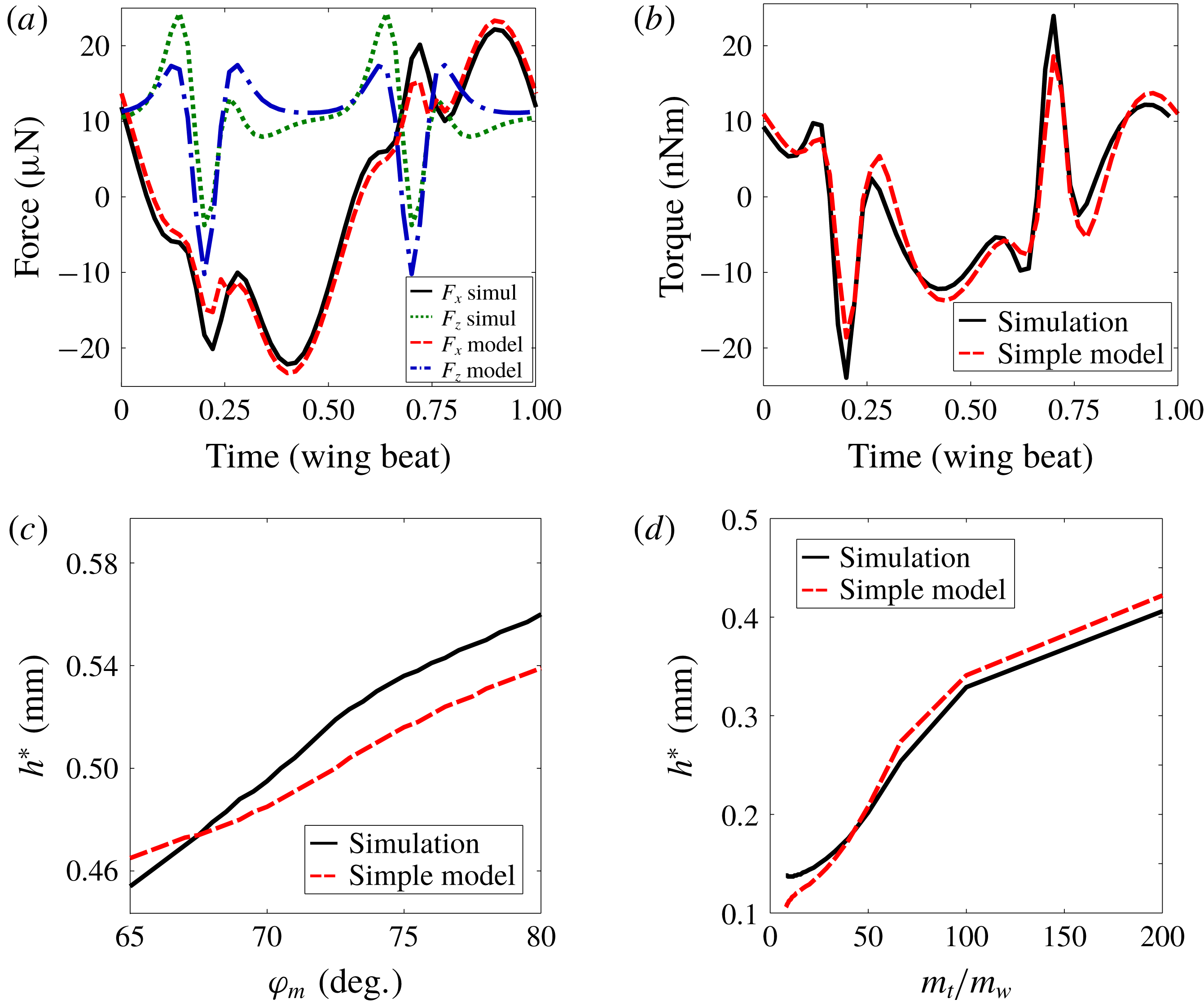
Comparing the simple model and the simulation. (a) Instantaneous forces. (b) Instantaneous torque. (c) A zoomed-in view of optimal hinge position as a function of the stroke amplitude. Both the simulation and the simple model show a slight increase with
 $h^{\ast }$
. (d) Numerical checks of the prediction that
 $h^{\ast }\sim m_{t}/m_{w}$
in the large
 $m_{t}/m_{w}$
limit.

Finally, we include the comparison between the simple model and the simulation, as well as the numerical checks of the prediction made in (3.11). The point mass model captures the main features in the forces and the torque given by the simulation (figure 4
a,b). The difference in the time series is partly due to the assumption of a constant lift in the reduced order model. The optimal hinge position
 $h^{\ast }$
from the simple model are also similar to the simulation results, both in the dependence on amplitude (figure 4
c) and on the wing mass to body mass ratio (figure 4
d). The optimal hinge position
 $h^{\ast }$
from the simple model are similar to the simulation results, both in the dependence on amplitude (figure 4
c) and on the wing mass to body mass ratio (figure 4
d). The model works well as long as the wings are lighter compared to the body, as is the case with insects.
4 Discussion
We have shown that the hinge position can be tuned to minimize body oscillation due to flapping motion. At this optimal hinge position, the ascending speed is maximized for a given stroke amplitude. The predicted optimal hinge position is approximately half-way between the centre of mass and the top of the body and is independent of the stroke amplitude.
Incidentally, the body–wing coupling discussed here also suggests a method for pitch control, which is to hold the wings still briefly during the wing beat. It is easiest to pause the wings at the wing reversal. This brief pause is most effective when the body velocity is large. Thus the optimal phase delay between the body and the wing is
 $90^{\circ }$
, exactly the delay at anti-resonance.
Acknowledgement
Z.J.W. is grateful to the support of the Simon Fellowship from Newton Institute, Cambridge during the completion of the manuscript.