2.1. PIC simulations

The transverse dynamics of the electron plasma is simulated using a recently developed 2D PIC code (Maero et al. Reference Maero, Romé, Lepreti and Cavenago2014). The code simulates in general the 2D dynamics of a multispecies plasma in the plane orthogonal to a homogeneous magnetic field, implementing a massless fluid approximation for electrons and a kinetic description for the massive components. For the simulations presented here, however, only the electron population is considered.

It is worth noting that, in the case of a pure electron plasma, an Eulerian fluid numerical code could also be used to describe the dynamics of the system (Romé et al. Reference Romé, Brunetti, Califano, Pegoraro and Pozzoli2000), and the Eulerian fluid description would be cleaner from noise than the PIC one. However, the PIC code used here provides us with great flexibility, namely we can (a) easily adapt the boundary geometry and initial conditions and (b) use both fluid and kinetic trajectory integration routines for different particle populations. The latter feature can be particularly important, e.g. in order to compare the turbulence properties of a pure electron plasma with those of a dust-contaminated electron plasma, where dust grains require a kinetic treatment (Maero et al. Reference Maero, Romé, Lepreti and Cavenago2014). Moreover, the PIC noise is useful in the present context to simulate the non-uniformities of the initial electron distribution that are unavoidably present in the experiments, and their influence on the late evolution of the system (see § 3.3).

The plasma domain is supposed to be bounded by a (perfectly) conducting wall of radius  $R_{w}$ . The electrostatic potential ${\it\phi}$ is therefore set to zero on the circular boundary. This corresponds to free-slip boundary conditions in the fluid description. In the PIC code, a Cartesian $N_{\mathit{grid}}\times N_{\mathit{grid}}$ grid, with $N_{\mathit{grid}}=256$ , is used, and the circular boundary is approximated by a piecewise linear function following the sides of the mesh cells. The number of macro-particles, $N_{\mathit{macro}}$ , is  $10^{6}$ . Using a standard bilinear interpolation for the charge density, the Poisson equation for ${\it\phi}$ is solved by means of a 2D fast Fourier transform (FFT) combined with a capacity matrix method (Hockney & Eastwood Reference Hockney and Eastwood1981). For the time advancement of the electrons, a fourth-order Runge–Kutta algorithm is adopted.

Equations (1.1) can be written in non-dimensional form as

where the density $n$ is normalized over a reference value $n_{0}$ , the lengths over the trap radius $R_{w}$ , the electrostatic potential ${\it\phi}$ over $en_{0}R_{w}^{2}/{\it\epsilon}_{0}$ and the time over ${\it\omega}_{c}/{\it\omega}_{p}^{2}={\it\epsilon}_{0}B/en_{0}$ , where ${\it\omega}_{c}=eB/m$ is the (non-relativistic) electron cyclotron frequency and ${\it\omega}_{p}=(e^{2}n_{0}/{\it\epsilon}_{0}m)^{1/2}$ is the plasma frequency computed using the density $n_{0}$ . Simulations performed for the same final time therefore correspond to a given ratio between the density and the magnetic field strength. In the following, only non-dimensional quantities are used. The parameters of the simulations presented here are analogous to those used (in dimensional form) in (Maero et al. Reference Maero, Romé, Lepreti and Cavenago2014), and correspond to experimental conditions actually encountered in existing or planned Penning–Malmberg traps (Maggiore et al. Reference Maggiore, Cavenago, Comunian, Chirulotto, Galatà, De Lazzari, Porcellato, Roncolato, Stark, Caruso, Longhitano, Cavaliere, Maero, Paroli, Pozzoli and Romé2014; Romé et al. Reference Romé, Cavaliere, Cavenago, Chen and Maero2015).

The drift Poisson system (2.1) is Hamiltonian and expresses the fact that the electron density (fluid vorticity) is a Lagrangian invariant, i.e. it is constant along the characteristics given by the $E\times B$ drift. The evolution of the electron density is constrained by an infinite number of constants of motion, known as Casimirs (Morrison Reference Morrison1984), corresponding to integrals over the spatial domain of an arbitrary function of the Lagrangian invariant density. In particular, the enstrophy (Leith Reference Leith1968) corresponds to the quadratic invariant

where $(r,{\it\theta})$ are polar coordinates defined in the circular domain. These Casimirs are conserved in addition to the total number of particles $N_{\mathit{tot}}$ , the energy $H$ and the angular momentum $P_{{\it\theta}}$ (all these quantities are defined per unit axial length). In non-dimensional form these are given by

In the fluid analogy, the corresponding quantities are the total circulation, the excess kinetic energy and the total angular impulse, respectively (Melander et al. Reference Melander, Zabusky and McWilliams1988). In the simulations presented here, $H$ and $P_{{\it\theta}}$ are typically conserved with a relative accuracy of the order of $10^{-5}$ and $10^{-6}$ , respectively, for a time equivalent to more than a hundred plasma rotation periods. On the contrary, the total enstrophy $Z$ and in general all other higher moments of the vorticity tend to decrease with time. This effect is due to ‘coarse-graining’, as observed both in experiments and in numerical simulations (Schecter et al. Reference Schecter, Dubin, Fine and Driscoll1999): the density (vorticity) filaments become longer and longer so that their thickness becomes smaller than the experimental resolution (e.g. the pixel size of the optical diagnostics of the density) or smaller than the cell size of the numerical mesh used for the discretization of the 2D Euler equations, respectively. This effect of coarse-graining on the invariants of the 2D Euler equations has been pointed out also in statistical treatments of the 2D turbulence (Miller Reference Miller1990).

The initial electron density distribution is assumed to be uniform over an annular region. This kind of density distribution can be easily produced in the experiments (Peurrung & Fajans Reference Peurrung and Fajans1993) and it also allows for a quantitative comparison with analytical results of the linear evolution stage of azimuthal low-frequency instabilities of the system (Davidson Reference Davidson1990). In order to investigate the influence of the initial distribution on the evolution of the plasma turbulence, the same uniform density and the same total number of particles $N_{\mathit{tot}}$ are considered in all simulations. This is accomplished by keeping the total initial area $A$ covered by the plasmas constant, and varying the outer radius $r^{+}$ of the annulus (and correspondingly its inner radius  $r^{-}$ ) in a given range. As a reference value, $A=0.0729{\rm\pi}$ has been chosen, i.e. a fraction of slightly more than 7 % of the total cross-section of the trap is supposed to be initially filled by the plasma. The various cases therefore differ for the profile of the shear of the rotation angular frequency, $r\,\text{d}{\it\omega}_{r}/\text{d}r=(r^{-}/r)^{2}$ , inside the plasma (the rotation frequency ${\it\omega}_{r}$ being normalized over ${\it\omega}_{p}^{2}/{\it\omega}_{c}$ ), and for the value of the canonical angular momentum $P_{{\it\theta}}$ and of the energy  $H$ . With $N_{\mathit{macro}}=10^{6}$ , the number of simulation particles per occupied cell for the initial condition is typically greater than 250, which guarantees a good level of density uniformity over the area initially covered by the plasma (see discussion on this point in § 3.3).

2.2. Wavelet multiresolution analysis

A wavelet-based MRA method is applied in order to separate the coherent structures (persistent vortices) from the incoherent vorticity distribution and to perform a spectral analysis on the coherent and incoherent parts of the flow. The ‘signal’, i.e. the 2D vorticity (density) distribution at a given time of the evolution, is successively decomposed into coefficients that contain coarse and fine details at increasingly finer resolution. The 2D vorticity field is expanded as

i.e. as a linear combination of elementary well-localized functions ${\it\psi}_{j,i_{x},i_{y}}^{{\it\sigma}}(x,y)$ (here a Symlet8 wavelet has been chosen), with coefficients $\tilde{{\it\zeta}}_{j,i_{x},i_{y}}^{{\it\sigma}}$ . These wavelet coefficients are then separated into coherent and incoherent parts, using an adaptive, self-consistent universal Donoho’s threshold within an iterative method (Farge, Schneider & Kevlahan Reference Farge, Schneider and Kevlahan1999; Ruppert-Felsot, Farge & Petitjeans Reference Ruppert-Felsot, Farge and Petitjeans2009). The method is similar to the one applied in a previous work (Bettega, Pozzoli & Romé Reference Bettega, Pozzoli and Romé2009) for the analysis of experimental time sequences of the electron density distribution, where it was shown that most of the information about the 2D flow is retained in a small fraction of the coefficients describing the coherent part.

In the present work, the method has been modified in order to take into account a possible inhomogeneity of the incoherent part. In the usually adopted method (Ruppert-Felsot et al. Reference Ruppert-Felsot, Farge and Petitjeans2009), the incoherent part ${\it\zeta}_{{<}}$ at the $i$ th iteration step is reconstructed using wavelet coefficients smaller (in absolute value) than a threshold ${\it\epsilon}_{T}^{(i)}$ (which is computed at the previous step). Its variance $\langle {\it\zeta}_{{<}}^{2}\rangle =(1/N_{\mathit{grid}}^{2})\sum {\it\zeta}_{{<}}^{2}(x,y)$ is then used to compute the new threshold ${\it\epsilon}_{T}^{(i+1)}=(2\langle {\it\zeta}_{{<}}^{2}\rangle \log N_{\mathit{grid}}^{2})^{1/2}$ at the next step. At the first iteration, ${\it\epsilon}_{T}^{(1)}=(2\langle {\it\zeta}^{2}\rangle \log N_{\mathit{grid}}^{2})^{1/2}$ , where $\langle {\it\zeta}^{2}\rangle$ is the variance of the total signal. The method works well, i.e. the threshold stabilizes (indicating convergence) after a few iterations, $|{\it\epsilon}_{T}^{(i+1)}-{\it\epsilon}_{T}^{(i)}|\approx 0$ , and the coherent and incoherent parts are then separated, for the cases where the incoherent part can be regarded as an additive Gaussian noise homogeneously distributed over all grid points. However, if the incoherent part is highly inhomogeneous and actually covers only a small fraction of the grid points, the threshold fails to converge. The reason for this failure is as follows. On the one hand, convergence of the threshold requires the variance of the incoherent part $\langle {\it\zeta}_{{<}}^{2}\rangle$ to be similar to the intrinsic variance ${\it\sigma}_{G}^{2}$ of a Gaussian noise. On the other hand, $\langle {\it\zeta}_{{<}}^{2}\rangle$ (and thus  ${\it\epsilon}_{T}$ ) depends not only on its intrinsic statistical properties, but also on a geometric factor: the ratio of the area covered by the incoherent part to the total signal domain. When the incoherent part is distributed over all (or most of) the grid points, this ratio is approximately equal to 1, and $\langle {\it\zeta}_{{<}}^{2}\rangle \approx {\it\sigma}_{G}^{2}$ . If, however, the incoherent part is inhomogeneously distributed, the geometric factor can be much smaller than 1 (e.g. at the initial time it is approximately 7 %, as mentioned above, since it corresponds to the percentage of the domain where the signal is effectively non-zero), resulting in $\langle {\it\zeta}_{{<}}^{2}\rangle \ll {\it\sigma}_{G}^{2}$ . In the latter case, the requirement for the threshold convergence is violated and the algorithm fails. In order to relax this restriction, we considered at each step the relative change of the threshold, ${\rm\Delta}\hat{{\it\epsilon}}_{T}^{(i)}=[{\it\epsilon}_{T}^{(i+1)}-{\it\epsilon}_{T}^{(i)}]/{\it\epsilon}_{T}^{(i)}$ . Unlike ${\it\epsilon}_{T}$ , ${\rm\Delta}\hat{{\it\epsilon}}_{T}$ does not depend on the geometric factor, and ensures that at a certain step $|{\rm\Delta}\hat{{\it\epsilon}}_{T}^{(i_{0}+1)}-{\rm\Delta}\hat{{\it\epsilon}}_{T}^{(i_{0})}|\approx 0$ . Then we can use the corresponding threshold ${\it\epsilon}_{T}^{(i_{0})}$ to separate the coherent and incoherent parts. Using this modified algorithm, we can retain the hypothesis of Gaussianity of the incoherent part, while relaxing the requirement that it covers the entire signal domain.

Figure 1.

Results of the modified wavelet MRA for $r^{+}=0.40$ . The top, middle and bottom rows show the absolute values of the total, coherent and incoherent parts, respectively. In each plot the data are normalized to their respective maximum values. Each column corresponds to a different time, namely $t=0$ , 90, 180, 270 and 360, as indicated at the upper-left corner of each plot in the top row.

To demonstrate its performance, we present in figure 1 the results of this modified algorithm applied to the case of $r^{+}=0.40$ . The top, middle and bottom rows show the absolute values of the total, coherent and incoherent parts of the density distribution, respectively, while each column corresponds to a different time. For the sake of clarity, all distributions are normalized to their respective maximum values. The evolution of the total and/or the coherent vorticity field will be discussed in detail in the following sections. The incoherent part is inhomogeneous at early times (e.g.  $t=0$ and 90), but acquires a higher degree of homogeneity at later times (from $t=180$ to 360). On the other hand, the values of the incoherent part turn out to be randomly distributed throughout all the time evolution. These features confirm that the modified algorithm described above is able to separate the inhomogeneous incoherent part. It is also worth noting that, as the system evolves towards its final state, a nearly uniform turbulent background is formed, even in the presence of a central vortex patch. This result will be discussed further in § 3.2. Further technical details about the modified method of separation of the coherent and incoherent parts of the flow will be reported in a future paper. Despite its possible inhomogeneity, the incoherent part can still be considered as a Gaussian noise, and the main interest of the present work remains in the coherent part.

3.1. Emergence of different final states

As mentioned in the previous section, we choose the outer radius $r^{+}$ of the annulus as the freely varying parameter. A series of simulations are performed in which $r^{+}$ is systematically changed from 0.35 to 0.46 with an increment of 0.01. The evolutions of the vorticity for different values of $r^{+}$ are shown in figure 2. Each row corresponds to a given value of  $r^{+}$ , while each column corresponds to a different time.

Figure 2.

Time evolutions of the electron density (vorticity). Each row corresponds to a given value of the outer radius of the initial annulus: $r^{+}=0.35$ , 0.40, 0.45 and 0.46 (last two rows). Each column corresponds to a different (normalized) time, as indicated at the upper left corner of each plot in the first row.

The numerical results show in general typical fluid phenomena like the development of the diocotron instability (Kelvin–Helmholtz instability in the fluid language), vortex merging events, the emission of vorticity filaments and the development of a turbulent background. In all cases there is a first stage characterized by the development of the diocotron instability, which leads to the breakup of the annulus into several vortices. After this stage, however, the evolution of plasma changes drastically as $r^{+}$ increases, leading to quite different final states. For smaller  $r^{+}$ , the final state consists of a single central patch and a turbulent background, while for larger $r^{+}$ final states with multiple vortices can emerge.

We have performed an analysis of the early evolution of the diocotron instability to extract the growth rate ${\it\gamma}_{l}$ of the $l$ th mode from the simulation data and to compare the results with the theoretical predictions based on a linear perturbation analysis (Davidson Reference Davidson1990). The electron density and the electrostatic potential at any time $t$ can be Fourier-analysed as

where ${\it\omega}_{l}$ is a complex frequency. The diocotron mode of order $l$ is unstable if ${\it\gamma}_{l}=\text{Im}({\it\omega}_{l})>0$ : this also defines the growth rate of the mode. Accordingly, the electrostatic energy contained in the $l$ th mode is

where the asterisk denotes the complex conjugate. In practice, the density and potential at time $t$ are calculated on a polar grid starting from the instantaneous particle distributions, and their Fourier components are used to evaluate the electrostatic energy $E_{l}(t)$ . Fitting $E_{l}(t)$ to an exponential function yields the growth rate $2{\it\gamma}_{l}$ . Alternatively, one can calculate the power $A_{l}(t)$ of the $l$ th mode,

where ${\it\delta}{\it\phi}_{l}(r,t)$ denotes the $l$ th Fourier component of the potential perturbation, and carry out a similar exponential fitting of $A_{l}(t)$ (Maero et al. Reference Maero, Romé, Lepreti and Cavenago2014). The numerical growth rates obtained by these two methods agree well with each other, and hereafter we report the results obtained using the former one.

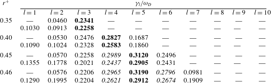
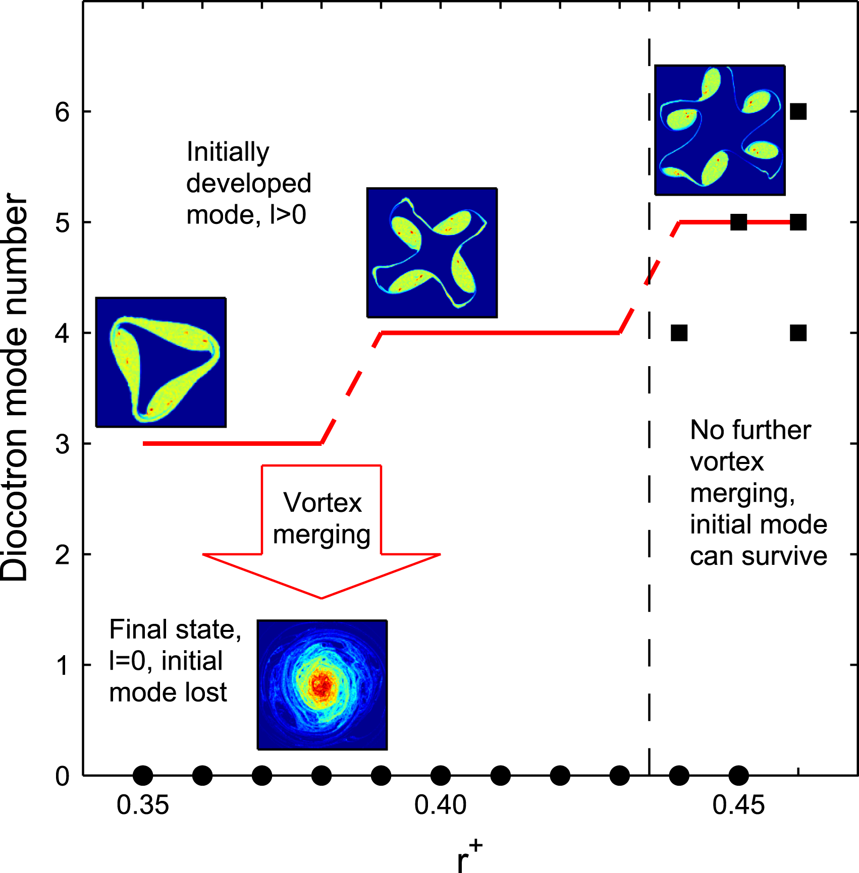
In table 1 we list the exponential growth rates ${\it\gamma}_{l}$ for $l=1{-}10$ for a few values of  $r^{+}$ . The growth rates are normalized by the diocotron frequency ${\it\omega}_{D}={\it\omega}_{p}^{2}/2{\it\omega}_{c}$ . The dominant mode (indicated in bold) progressively changes from $l=3$ to $l=4$ and finally to $l=5$ . In figure 3 we plot the dominant diocotron mode number in the final state versus the outer radius  $r^{+}$ . The solid circles represent final states with a single central vortex. Since these states are approximately axisymmetric, they are characterized by $l=0$ . The solid squares, on the contrary, represent multiple-vortex final states with non-zero mode numbers. Representative vorticity distributions during the diocotron instability stage are also shown (see insets). It is well known that the instability occurs at higher azimuthal mode numbers when the plasma annulus becomes thinner (Davidson Reference Davidson1990). In the present study, as $r^{+}$ increases, the width of the annulus decreases, and the mode with the largest growth rate therefore shifts to a higher  $l$ . It turns out that, for cases with low-order dominant diocotron modes, vortex merging processes dominate the plasma evolution up to the formation of a single central vortex. In the opposite case, i.e. for higher-order dominant diocotron modes, vortex merging processes can be largely suppressed, and the initially dominant mode leads to the formation of a chain of vortices (vortex crystal), characterized by a number of vortices equal to the order of the same dominant mode.

Figure 3.

Azimuthal mode number of the dominant diocotron mode in the final state versus the normalized outer radius  $r^{+}$ . The solid circles and squares represent final states with a single central vortex and with multiple vortices, respectively. The red lines indicate the dominant modes for different $r^{+}$ as predicted from the linear theory (Davidson Reference Davidson1990). Insets show examples of vorticity distributions during the diocotron instability stage.

Table 1.

Growth rate ${\it\gamma}_{l}$ (normalized to ${\it\omega}_{D}$ ) of the diocotron modes for different values of  $r^{+}$ . For each radius, the values in the first row are the analytical predictions of the linear perturbation theory (Davidson Reference Davidson1990), while the values in the second row are obtained by the Fourier analysis of the results of the numerical simulations. The growth rate of the dominant mode is indicated in bold. The growth rates of other modes that are only slightly smaller than that of the dominant one are indicated in italic. Stable modes are represented by dashes.

In order to investigate in more detail the time evolution of the plasma turbulence, we compare the vorticity distribution as well as the enstrophy spectrum of the coherent part for two qualitatively different cases, namely $r^{+}=0.40$ and $r^{+}=0.46$ . The maximum wavenumber $k_{\mathit{max}}$ of the spectrum is the inverse of the minimum spatial scale of the wavelet functions (which is twice the length of a grid cell), i.e.  $k_{\mathit{max}}=1/[2\times (2/N_{\mathit{grid}})]=64$ (the wavenumber is normalized over the inverse of the trap wall radius, $1/R_{w}$ ). In each successive decomposition level the spatial scale of the wavelet functions is increased by a factor of 2 and $k$ is accordingly divided by 2, up to a maximum level of $(\log _{2}N_{\mathit{grid}}-1)=7$ , i.e. up to a minimum wavenumber $k_{\mathit{min}}=1$ .

Figure 4.

Comparison of vorticity distribution and enstrophy spectrum of the coherent part between (a)  $r^{+}=0.40$ and (b)  $r^{+}=0.46$ . The enstrophy spectrum is normalized by its maximum value at each time. In (a), the three main stages (i.e. development of diocotron instability, vortex merging and final state) are separated by two vertical dashed lines, while in (b) the vortex merging stage is absent.

For $r^{+}=0.40$ (see figure 4 a), we can distinguish three main stages. The first stage corresponds to the above-mentioned evolution of the diocotron instability, during which the annulus breaks into multiple (e.g. four in this case) vortices. The second stage lasts until the formation of a single vortex state. During this stage the vortices interact strongly with each other, undergoing vortex merging and emission of vorticity filaments. As a consequence of these processes, the vortices collapse into a single central patch, and a significant turbulent background is formed. It is worth noting that this stage can be distinguished not only from the visible evolution of the vorticity distribution, but also from a ‘bifurcation’ structure in the coherent enstrophy spectrum (as discussed in detail in § 3.2). After this stage both the vorticity distribution and the coherent enstrophy spectrum remain relatively stable, without further evolution. On the other hand, it is clear from figure 4(b) that for $r^{+}=0.46$ the second stage is absent. The multiple vortices formed after the diocotron instability evolution do not merge with each other and the emission of the vorticity filaments is greatly reduced.

3.2. Development of turbulence

As mentioned before, during the vortex merging stage the vortices generated from the diocotron instability interact with each other, collapse into a central vortex, and generate a strong turbulent background. This implies that the vortex merging process is closely related to the development of turbulence, as discussed in the following.

Figure 5.

Coherent enstrophy spectrum for different initial outer radii of the plasma annulus, as indicated at the upper left corner of each plot. The spectrum is normalized by its maximum value at each time. The vortex merging stage corresponds to the period in which the spectrum shows a bifurcating structure. When the vortex filaments lose their identity into a turbulent background, the upper branch at larger wavenumbers disappears. The instant at which the upper branch falls completely below the value 0.5 (indicated by the black contour lines) is regarded as the typical time of turbulence development, $T_{\mathit{turb}}$ (indicated by the white dashed lines).

In figure 5 we compare the evolution of the enstrophy spectrum of the coherent component for different  $r^{+}$ . A common feature is that the vortex merging stage corresponds to the period in which the spectrum shows a ‘bifurcation’ structure. During the diocotron instability stage, the annulus breaks into several vortices, but the spatial scale of these vortices remains roughly the same as that of the annulus. Therefore, the peak of the enstrophy spectrum (indicated by the red region) remains close to its initial position during this period. However, during the merging process the vortices become highly deformed, and emit vortex filaments. In the meantime the enstrophy is transferred into components of both larger (central vortex) and smaller (vortex filaments) spatial scales. This corresponds to the bifurcation of the spectrum. At the end of the merging stage, vortex filaments evolve into a turbulent background, losing their identity. Thus, the upper branch at larger wavenumbers (i.e. smaller spatial scales) disappears in the spectrum of the coherent part of the flow and only the lower branch at smaller wavenumbers (i.e. larger spatial scales) remains. The time $T_{\mathit{turb}}$ at which the upper branch vanishes can be regarded as the typical time of turbulence development. This time is estimated from the coherent enstrophy spectrum as the instant at which the upper branch falls completely below a given value, which we set here to 0.5. Notice the black contour lines for the level 0.5 and the white dashed lines indicating $T_{\mathit{turb}}$ in figure 5.

The comparison between the spectrum evolution for different initial outer radii in figure 5 implies that $T_{\mathit{turb}}$ increases with  $r^{+}$ . In figure 6 we show the relation between $T_{\mathit{turb}}$ and  $r^{+}$ . Several (at least four) simulations are actually carried out for a given  $r^{+}$ , so that the average of the values of $T_{\mathit{turb}}$ obtained in all these simulations is shown in the plot, together with an error bar corresponding to one standard deviation. It is confirmed that, as $r^{+}$ increases, it takes more time for turbulence to fully develop. Several considerations qualitatively support and clarify this evidence. First, as the outer radius increases, the effective area that can be covered by the turbulent background also increases. Namely, the vortex filaments become thinner and thinner with time and the strong vortices tend to move towards the centre, while the canonical angular momentum of the system is kept constant during the evolution. This effect explains the growth of $T_{\mathit{turb}}$ since the time needed to obtain an almost uniform background increases, as already shown in figure 1. Second, as the dominant mode shifts to higher mode numbers, more vortices are generated before the vortex merging stage actually begins. The typical size of these vortices becomes smaller, while the average distance between the vortices gets larger, so that it takes more time for vortex merging to complete, and the evolution of turbulence is slowed down. This effect contributes to the increase of the slope of $T_{\mathit{turb}}$ with  $r^{+}$ . One can also consider that the area to be covered by the turbulent background increases with the square of $r^{+}$ and it is therefore reasonable to expect a quadratic trend for  $T_{\mathit{turb}}$ . Indeed, the solid fitted line in figure 6 shows that the data are compatible with a quadratic dependence with the outer ring radius.

Figure 6.

Relation between the typical time of turbulence development $T_{\mathit{turb}}$ and the outer radius  $r^{+}$ . The solid line is a quadratic fit.

3.3. Effect of initial fluctuations

In the PIC simulations the initial particle positions are given using a Mersenne Twister (Matsumoto & Nishimura Reference Matsumoto and Nishimura1998) random number generator (RNG). As with any RNG, fluctuations are introduced into the initial density distribution. To estimate the degree of non-uniformity of the initial particle distribution, we computed for different geometries and different $N_{\mathit{macro}}$ the distributions of the number of macro-particles per cell. Indicating with $n_{i}$ the number of macro-particles in the $i$ th cell and with $\hat{n}$ its average value, the standard deviation ${\it\sigma}$ of the macro-particle distribution is computed as

where $N_{\mathit{cell}}$ is the number of grid cells over which the distribution of macro-particles is defined. As an example, in figure 7 the normalized standard deviation ${\it\sigma}/\hat{n}$ is shown for different values of $N_{\mathit{macro}}$ for a distribution in a square (square markers) and in a circular region (diamond markers), respectively. In both cases, $N_{\mathit{grid}}=256$ has been used and the particles have been generated in a test region located at the centre of the domain, covering about the same fraction of the total computational area as that initially covered by the plasma in the previously reported simulations. For the square distribution the boundary of the test region is assumed to coincide with the sides of the mesh cells.

Figure 7.

Standard deviation ${\it\sigma}$ of the macro-particle distribution normalized over the average number of macro-particles per cell $\hat{n}$ versus the total number of macro-particles $N_{\mathit{macro}}$ for a square (square markers) and a circular (diamond markers) distribution.

In the case of the square distribution, the relative standard deviation decreases as $1/\sqrt{N_{\mathit{macro }}}$ and is approximately 5 % for $N_{\mathit{macro}}=10^{6}$ , which is the number of macro-particles used in the simulations reported in the paper. In this case the fluctuations of the particle distribution are due simply to the intrinsic non-uniformity of the RNG. On the contrary, the decrease of ${\it\sigma}/\hat{n}$ with $N_{\mathit{macro}}$ turns out to be much slower in the case of the circular distribution. Here, the particles are covering a region whose boundary does not coincide with the sides of the mesh cells. In other words, the mesh cells located at the boundaries of the region occupied by the initial distribution have a smaller $n_{i}$ with respect to the cells in the interior. For a given $N_{\mathit{macro}}$ the average number of macro-particles per cell $\hat{n}$ is therefore reduced with respect to the square distribution and ${\it\sigma}$ increases. In this case the fluctuations of the particle distribution are mainly due to the discretization of the system.

Albeit almost unavoidable, these fluctuations have often been neglected or scarcely considered. The effect of fluctuations at lower macro-particle density can sometimes be masked by intentional spatial or density perturbations superimposed on the initial distributions, as customary in some studies of the diocotron instability (see for instance Delzanno et al. Reference Delzanno, Lapenta and Finn2002). Nevertheless, such imperfections may have a significant effect on the fluid dynamics, as we show in the following. Furthermore, although different in nature, they have an equivalent counterpart in real experiments, where particle sources have an intrinsically limited degree of uniformity and reproducibility. Hence the effect of initial fluctuation is not only of numerical interest, but also of practical significance (Yatsuyanagi et al. Reference Yatsuyanagi, Kiwamoto, Ebisuzaki, Hatori and Kato2003). It is found that for cases with small $r^{+}$ initial fluctuations have a negligible effect on the plasma evolution. The analysis of vorticity distribution, enstrophy spectrum, probability distribution function and other quantities shows only minor differences between different runs performed with the same macroscopic parameters. On the other hand, for cases with large $r^{+}$ , even very small initial fluctuations can lead to quite different plasma evolutions. For example, the results of four runs with $r^{+}=0.46$ are shown in figure 8: three runs end up with four vortices and one run with six vortices. A similar situation is observed for $r^{+}=0.45$ (not shown here), where the system evolves to a single central vortex in two runs, and to a final state with four vortices in two other runs.

Figure 8.

Effect of initial fluctuations for ‘sensitive’ cases where multiple competing diocotron modes exist. The red bars indicate the competing modes and the green ones the other modes. The competing mode with the largest initial energy (indicated by the arrow) survives in the final state (see insets).

Such an effect of initial fluctuations can be explained according to the diocotron instability theory. As shown in table 1, for small $r^{+}$ fewer modes are unstable and the growth rate of the dominant mode is much larger than that of all other modes. Thus it will always survive the diocotron instability stage, regardless of the presence of fluctuations. In these cases (which we call ‘insensitive’), the effect of initial fluctuations is negligible. For large  $r^{+}$ , on the other hand, the growth rate of the dominant mode is only slightly greater than that of the second and/or third fastest ones. Since these modes are competing, each of them has the possibility to survive the diocotron instability stage. In these cases (which we call ‘sensitive’), the development of the diocotron instability depends not only on the growth rate but also on the initial energy of these competing modes. In order to clarify this point, we take $r^{+}=0.46$ as an example, and use (3.3) to calculate the initial energies $E_{l}$ of the $l$ th mode for all four runs. As fluctuations eventually contribute to $l>0$ modes, $E_{l}$ with $l=1{-}9$ (normalized by the initial energy $E_{0}$ of the $l=0$ mode) are shown in figure 8. The competing modes are indicated by red bars. It is clear that the competing mode with the largest initial energy survives up to the final state, which confirms the effect of the initial fluctuations mentioned above.