3.1 Linear stability of the basic state

In this section we will in the first instance consider the linear stability of the basic state as the Görtler number varies. We assume that disturbances to the basic state are sufficiently small that nonlinear effects can be ignored, and then solving the resulting set of linearised equations we find either that the perturbations decay exponentially in time or space to zero in which case the flow is linearly stable, or the perturbations grow exponentially until nonlinear effects are no longer negligible. Linearising (2.6) we find

where ${\mathcal{L}}$ is defined in (2.5a,b ). Because these equations are linear we can decompose the solution into spanwise harmonics, each with a constant streamwise growth rate. For a spanwise wavenumber $\unicode[STIX]{x1D6FD}$ we write

where the temporal growth rate $\unicode[STIX]{x1D70E}$ , or the streamwise growth rate $\unicode[STIX]{x1D6FE}$ and the behaviour in the wall-normal direction are to be determined. For a given spanwise wavenumber the Görtler numbers for neutral temporal or spatial modes must of course coincide and since previous work has shown that the flow is convectively unstable it is more appropriate to consider spatial instability. However since the only available results for growth rates in the literature are for temporal instability, see Park & Huerre (Reference Park and Huerre1988), we will in the first instance consider that case and take $\unicode[STIX]{x1D6FE}=0$ . It is convenient to let ${\mathcal{L}}_{n}$ denote the linear operator ${\mathcal{L}}$ applied to the $n$ th spanwise harmonic so that we write

Substituting (3.2) into (3.1) and eliminating $\bar{w}$ we find

These are to be solved subject to no-slip boundary conditions on the wall and far-field decay conditions. The conditions for no slip on $\tilde{u}$ and $\tilde{v}$ are straightforward whilst continuity implies the vanishing of $\tilde{v}^{\prime }$ at the wall. The boundary conditions are therefore

Given a spanwise wavenumber $\unicode[STIX]{x1D6FD}$ and a Görtler number $G$ , equation (3.4) is either an eigenvalue problem for the streamwise growth rate $\unicode[STIX]{x1D6FE}$ or for the temporal growth rate $\unicode[STIX]{x1D70E}$ depending on whether we set $\unicode[STIX]{x1D70E}=0$ or $\unicode[STIX]{x1D6FE}=0$ . For a fixed spanwise wavenumber the sign of the real part of the streamwise/temporal growth rate indicates whether disturbances grow or decay. If we set $\unicode[STIX]{x1D6FE}=0$ then we find that temporal growth rates are real and there exists a neutral value of the Görtler number $G_{n}(\unicode[STIX]{x1D6FD})$ where $\unicode[STIX]{x1D70E}(\unicode[STIX]{x1D6FD},G)<0$ if $G<G_{n}$ and $\unicode[STIX]{x1D70E}(\unicode[STIX]{x1D6FD},G)>0$ if $G>G_{n}$ . We call the curve where $\unicode[STIX]{x1D70E}=\unicode[STIX]{x1D6FE}=0$ , denoted by $G_{n}(\unicode[STIX]{x1D6FD})$ , the neutral curve. If we minimise the neutral Görtler number $G_{n}(\unicode[STIX]{x1D6FD})$ over all spanwise wavenumbers a value for the critical Görtler number can be found. There is actually a family of such curves $G_{n}^{(n)}(\unicode[STIX]{x1D6FD})$ where we use $n$ to denote the $n$ th such curve. 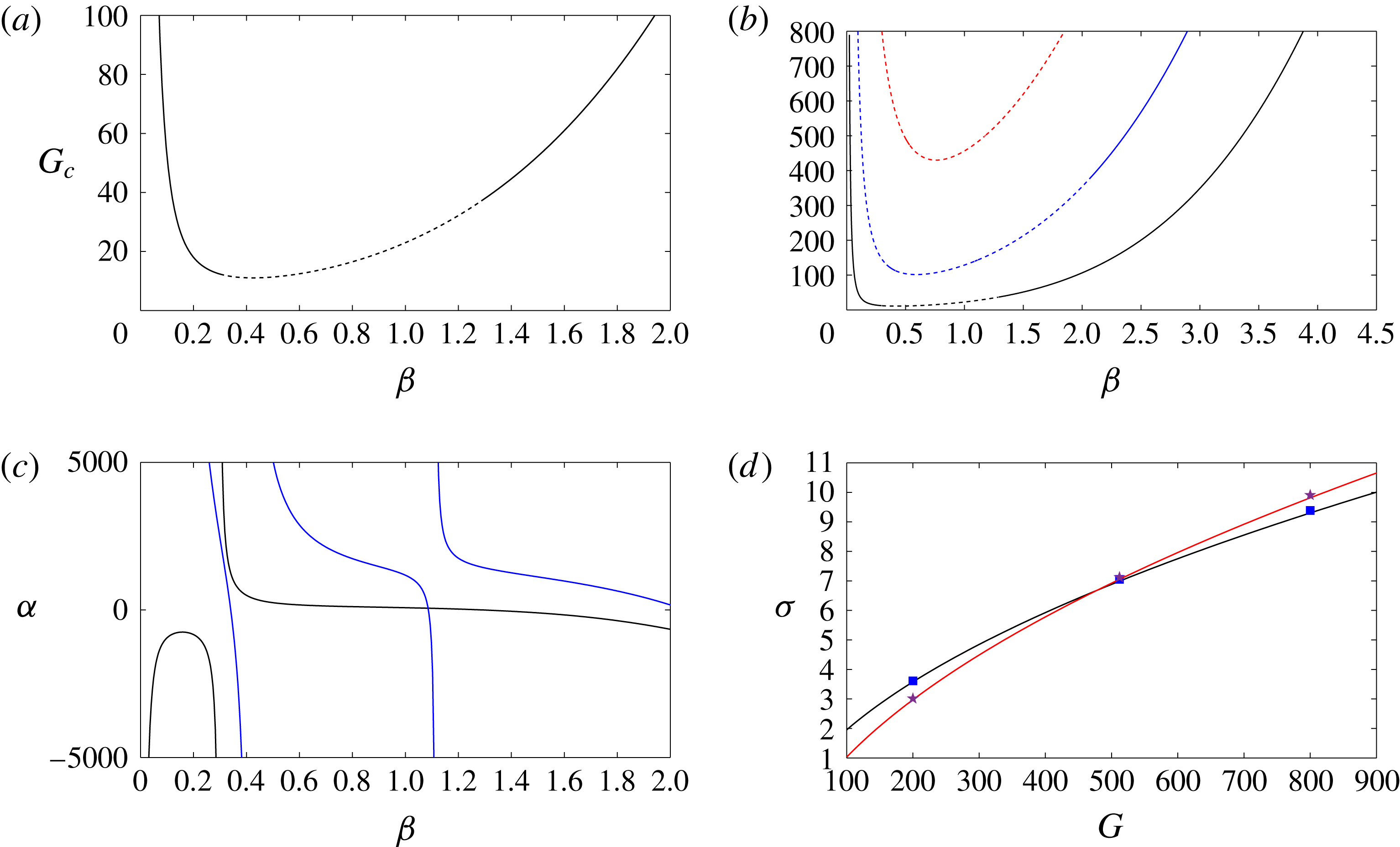It turns out that we can order these curves $0<G_{n}^{(1)}(\unicode[STIX]{x1D6FD})<G_{n}^{(2)}(\unicode[STIX]{x1D6FD})<\cdots \,$ ; see figure 1(a,b). For fixed spanwise wavenumber $\unicode[STIX]{x1D6FD}$ then, increasing the Görtler number $G$ through some $G_{n}^{(n)}(\unicode[STIX]{x1D6FD})$ signifies the basic state becoming linearly unstable to another family of eigenmodes of (3.4).

Figure 1.

The neutral curves and growth rate from the linear analysis. (a) $G_{n}^{(1)}(\unicode[STIX]{x1D6FD})$ : the first mode. A solid line denotes a supercritical bifurcation and a dashed line represents a subcritical bifurcation. (b) $G_{n}^{(n)}(\unicode[STIX]{x1D6FD})$ for $n=1$ (black), $n=2$ (blue), $n=3$ (red). The sub/supercritical nature of the bifurcations is denoted on this plot by line style as in (a). (c) $\unicode[STIX]{x1D6FC}(\unicode[STIX]{x1D6FD})$ : the Landau coefficient defined in (3.11) for the first two modes. The sign of $\unicode[STIX]{x1D6FC}$ indicates the criticality of the bifurcation as indicated by line style in (a,b). (d) $\unicode[STIX]{x1D70E}(G)$ : linear temporal growth rate for $\unicode[STIX]{x1D6FD}=1$ (black curve) and $\unicode[STIX]{x1D6FD}=1.6$ (red curve). Comparison with Park & Huerre (Reference Park and Huerre1995) for $\unicode[STIX]{x1D6FD}=1$ (blue squares) and $\unicode[STIX]{x1D6FD}=1.6$ (purple stars).

The eigenvalue problem is on a semi-infinite domain which for numerical purposes we approximate by replacing $\infty$ by $H$ . We then map the problem linearly onto the domain $[-1,1]$ where an expansion of the solution in Chebyshev polynomials is sought. The method of domain truncation combined with the use of Chebyshev polynomials was investigated by Boyd (Reference Boyd1982) where it was found to work well provided the function to be approximated is analytic. Although this method is straightforward to implement, one drawback is that improving the accuracy of the solution involves increasing $H$ and whenever this is done the number of Chebyshev polynomials used must also be increased. This does not cause any problems here where the structures are confined to a layer near the wall and decay sufficiently fast, but in § 3.4 when we consider fully nonlinear states of increasing amplitude these can now cover a much larger distance in the wall-normal direction resulting in the need to significantly increase $H$ . Applying the collocation method, the system of equations can now be written as a matrix $\unicode[STIX]{x1D648}$ times the vector of Chebyshev coefficients is equal to the zero vector. The matrix $\unicode[STIX]{x1D648}$ depends on the spanwise wavenumber and the neutral Görtler number, and non-zero solutions are possible only if the determinant of $\unicode[STIX]{x1D648}(\unicode[STIX]{x1D6FD},G_{n})$ is zero. Given a spanwise wavenumber $\unicode[STIX]{x1D6FD}$ , this determines $G_{n}$ and the Chebyshev coefficients of $\bar{u}$ and $\bar{v}$ can be determined by finding the zero eigenvector of $\unicode[STIX]{x1D648}(\unicode[STIX]{x1D6FD},G_{n}(\unicode[STIX]{x1D6FD}))$ . Figure 1(a) shows a plot of $G_{n}(\unicode[STIX]{x1D6FD})$ for the first mode, $G_{n}^{(1)}(\unicode[STIX]{x1D6FD})$ , where the differing line styles indicate whether the bifurcation is supercritical or subcritical; that issue will be discussed in § 3.2. Figure 1(b) is a plot of the first three modes, $G_{n}^{(n)}(\unicode[STIX]{x1D6FD})$ for $n=1,2$ and $3$ with the character of the bifurcations identified with differing line styles as in figure 1(a). The critical Görtler number corresponds to the turning point of the first mode and occurs where $G_{n}^{(1)}(\unicode[STIX]{x1D6FD})\simeq 16,\unicode[STIX]{x1D6FD}\simeq 0.4$ .

Park & Huerre (Reference Park and Huerre1995) considered, amongst other things, the temporal growth rate of Görtler vortices away from equilibrium; see table 1 of Park & Huerre (Reference Park and Huerre1995). Due to differences in the definition of the Görtler number and non-dimensionalisation, if we denote their definition of the Görtler number by $\bar{G}$ , spanwise wavenumber by $\bar{\unicode[STIX]{x1D6FD}}$ and temporal growth rate by $\bar{\unicode[STIX]{x1D70E}}$ then we find they are related to the analogous quantities used here by $\bar{G}=\sqrt{G/8}$ , $\bar{\unicode[STIX]{x1D6FD}}=\unicode[STIX]{x1D6FD}/2$ and $\bar{\unicode[STIX]{x1D70E}}=\unicode[STIX]{x1D70E}/4$ . Their paper documented the linear temporal growth rate for $\bar{\unicode[STIX]{x1D6FD}}=0.5$ ( $\unicode[STIX]{x1D6FD}=1$ ) and $\bar{\unicode[STIX]{x1D6FD}}=0.8$ ( $\unicode[STIX]{x1D6FD}=1.6$ ). 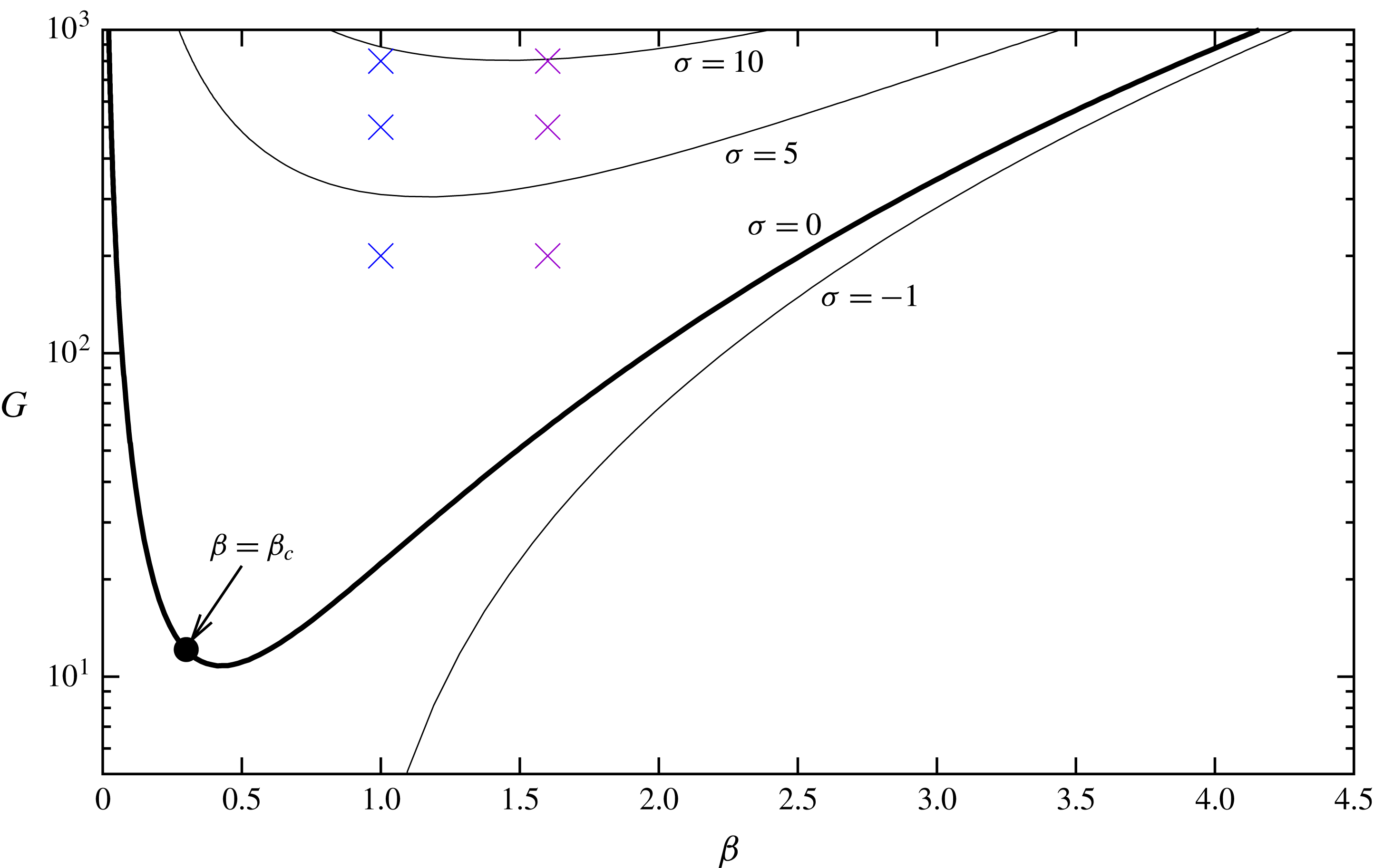In figure 1(d) we compare our results at those wavenumbers with the results of Park & Huerre (Reference Park and Huerre1995), excellent agreement between the two is observed. In figure 2 we show curves of constant growth rate in the $G-\unicode[STIX]{x1D6FD}$ plane. The points investigated by Park & Huerre (Reference Park and Huerre1995) are marked by crosses.

Next we consider the problem of finding small but finite amplitude equilibrium solutions in the vicinity of the neutral Görtler number. For convenience below we drop the superscript notation and unless stated otherwise below $G_{n}$ denotes the Görtler number of the first neutral mode. Here small amplitude solutions bifurcate from the linear neutral point. Since the growth rate is small close to the neutral curve the temporal and spatial growth rates differ only by a positive constant. Moreover the equations of motion are significantly simpler for the temporal problem and so for ease of exposition and following on from the discussion of temporal growth rates above we formulate the weakly nonlinear problem from a temporal viewpoint and point out the minor changes needed to be made to the final evolution equations to describe weak spatial evolution.

Figure 2.

Contours of constant growth rate in the $G-\unicode[STIX]{x1D6FD}$ plane. The crosses correspond to the point investigated by Park & Huerre (Reference Park and Huerre1995) and the circle denotes the point where the Landau coefficient becomes singular.

3.2 Weakly nonlinear analysis for general spanwise wavenumbers

We consider once again (2.6), but now account for finite amplitude effects. In particular the size of the disturbances will be such that the solutions are weakly nonlinear and, for the reasons stated above, we consider temporal rather than spatial evolution. However later when we consider the streamwise generation of vortices induced by free stream coherent structures we must use the spatial approach. Equations (2.6a )–(2.6e ) allow us to define a streamfunction $\unicode[STIX]{x1D6F9}$ by

so that (2.6) become

with no-slip boundary conditions on the wall and far-field decay given by

We will seek solutions to these equations which are periodic in the spanwise direction with spanwise wavenumber $\unicode[STIX]{x1D6FD}$ .

Consider the situation where the disturbance to the basic flow is small, say $O(\unicode[STIX]{x1D716})$ , and the Görtler number is close to the neutral value $G_{n}$ . We use a classic weakly nonlinear approach. This will require expansions for $\bar{u}$ and $\unicode[STIX]{x1D713}$ in terms of the spanwise harmonics. Consider the leading-order term in the expansions at $O(\unicode[STIX]{x1D716})$ , which consists solely of the first harmonic. As in § 3.1 we find the governing equations are the linearised form of (3.6), and hence non-trivial solutions exist only if the Görtler number $G$ is equal to the neutral Görtler number $G_{n}(\unicode[STIX]{x1D6FD})$ at leading order in $\unicode[STIX]{x1D716}$ . The $O(\unicode[STIX]{x1D716})$ components of $\bar{u},\unicode[STIX]{x1D6F9}$ are also determined up to an unknown amplitude, denoted by $A$ , which evolves over slow temporal or streamwise scales and will be determined at higher order. In fact $\bar{u}$ and $\unicode[STIX]{x1D6F9}$ are the eigenfunctions of the neutral (through the choice of $G$ ) linear problem. The analysis so far is identical to § 3.1 with $\unicode[STIX]{x1D70E}=\unicode[STIX]{x1D6FE}=0$ . This actually reaffirms our initial assumption that there is only one mode at leading order, because any other mode present say with spanwise wavenumber $\hat{\unicode[STIX]{x1D6FD}}$ would need to satisfy $G_{n}(\unicode[STIX]{x1D6FD})=G_{n}(\hat{\unicode[STIX]{x1D6FD}})$ (see § 3.3 where we will discuss a special case of this). The components at $O(\unicode[STIX]{x1D716})$ interact nonlinearly to generate terms at $O(\unicode[STIX]{x1D716}^{2})$ in the zeroth and second harmonic, and thus the expansion for $\bar{u},\unicode[STIX]{x1D6F9}$ at $O(\unicode[STIX]{x1D716}^{2})$ consists of the zeroth and second harmonics. At $O(\unicode[STIX]{x1D716}^{2})$ we find two independent linear problems for the zeroth and second harmonics which are forced by the first harmonic terms at $O(\unicode[STIX]{x1D716})$ . In general this set of equations can be solved (again, see § 3.3 for the exception). The nonlinear interaction of the first harmonic at $O(\unicode[STIX]{x1D716})$ and the zeroth and second harmonics at $O(\unicode[STIX]{x1D716}^{2})$ generates first and third harmonics at $O(\unicode[STIX]{x1D716}^{3})$ . As we will see, it is at $O(\unicode[STIX]{x1D716}^{3})$ where the interesting dynamics is determined and hence the critical curvature perturbation scale and slow time scale (given leading-order terms are $O(\unicode[STIX]{x1D716})$ ) are $G-G_{n}\sim O(\unicode[STIX]{x1D716}^{2})$ and $\unicode[STIX]{x2202}_{\bar{t}}\sim O(\unicode[STIX]{x1D716}^{2})$ . If we consider only the problem for the first harmonic at $O(\unicode[STIX]{x1D716}^{3})$ then we find that the homogeneous part of the operator is identical to the linear operator found at $O(\unicode[STIX]{x1D716})$ . However, the problem at $O(\unicode[STIX]{x1D716}^{3})$ is forced by the nonlinear interaction of the lower-order terms, and thus a solvability condition is found which determines the evolution equation for the amplitude $A$ . Motivated by the above argument we introduce new parameters which measure variations on the scales of interest as derived above. We let $G_{1}$ denote variations of the Görtler number on the $O(\unicode[STIX]{x1D716}^{2})$ scale, and $\unicode[STIX]{x1D70F}$ denote variations in the slow time scale $O(\unicode[STIX]{x1D716}^{-2})$ so we write

Exploiting symmetries in the spanwise direction the weakly nonlinear expansion, up to $O(\unicode[STIX]{x1D716}^{3})$ , is of the form

We then substitute the above expansions into (3.6) and equate successive powers of $\unicode[STIX]{x1D716}$ . At leading order we recover the linear neutral problem. At next order, inhomogeneous problems for the first harmonic and mean flow correction are found whilst finally at order $\unicode[STIX]{x1D716}^{3}$ the amplitude $A$ is determined as a solvability condition. Full details of the solution can be found in Dempsey (Reference Dempsey2015) and so we do not give them here. Note that in centrifugal instabilities there is no leading induced pressure field; see for example Hall (Reference Hall1988). We find that the required solvability condition takes the form

where $\unicode[STIX]{x1D707}_{1}$ and $\unicode[STIX]{x1D707}_{2}$ are constants defined in terms of integrals involving the leading-order eigenfunction and its adjoint. For the spatial problem the time derivative is replaced by a spatial one and $\unicode[STIX]{x1D707}_{1},\unicode[STIX]{x1D707}_{2}$ are multiplied by the same positive constant. If we restrict our attention to equilibrium solutions, $\unicode[STIX]{x2202}_{\unicode[STIX]{x1D70F}}=0$ , then we find the equilibrium amplitudes must satisfy

The unperturbed state of course corresponds to the equilibrium solution of this equation with zero amplitude. Once we have found the equilibrium states $A_{eq}$ , equation (3.9) can be used to determine the stability properties of each of the equilibrium solutions. The equilibrium solutions $A_{eq}$ and their stability are discussed later.

Varying the spanwise wavenumber is found to change the character of the bifurcation in $(G_{1},A)$ space. When $A$ is increased from zero, we call the bifurcation subcritical if $G_{1}$ decreases and supercritical if $G_{1}$ increases. Given the equilibrium solutions are $A_{eq}=0$ and $A_{eq}^{2}=-G_{1}/\unicode[STIX]{x1D6FC}$ where

the nature of the bifurcation is clearly determined by the sign of $\unicode[STIX]{x1D6FC}$ which denotes the Landau coefficient. In figure 1(a,b) we have indicated the character of the bifurcation fixed by the sign of $\unicode[STIX]{x1D6FC}$ which is plotted in figure 1(c). A solid curve is used when $\unicode[STIX]{x1D6FC}<0$ and the bifurcation is supercritical, and a dashed line is used when $\unicode[STIX]{x1D6FC}>0$ and the bifurcation is subcritical. For the primary branch, two sign changes of the Landau coefficient are observed for $\unicode[STIX]{x1D6FD}\in (0,2)$ , and hence as the spanwise wavenumber increases the bifurcation goes from supercritical to subcritical and back to supercritical over this range of spanwise wavenumbers. At the second of these points, $\unicode[STIX]{x1D6FD}\approx 1.3$ the Landau coefficient passes through zero smoothly. However, at the first of the critical points, $\unicode[STIX]{x1D6FD}=\unicode[STIX]{x1D6FD}_{c}\approx 0.30$ , the change in sign is due to the Landau coefficient blowing up. Clearly the weakly nonlinear analysis given in this section breaks down here, and it turns out that we must revisit our assumption that the leading-order expansion at $O(\unicode[STIX]{x1D716})$ consists of only a single harmonic. The fact that Görtler vortices in the asymptotic suction boundary layer bifurcate subcritically at the most dangerous wavenumber is quite unexpected based on well-known results for the closely related Taylor vortex problem. For growing boundary layers the most dangerous wavenumber is in the non-parallel regime but simulations by Hall (Reference Hall1988) show no sign of a subcritical behaviour. However in the latter problem the local wavenumber and Görtler number vary in the streamwise direction and Hall (Reference Hall1988) gave calculations for a limited range of initial disturbance. It should also be pointed out that subcritical instability for Tollmien–Schlichting waves in asymptotic suction flow was found by Hocking (Reference Hocking1975); but such a result for Tollmien–Schlichting waves is common whilst for centrifugal instabilities it is unusual.

3.3 Weakly nonlinear analysis for near-resonant spanwise wavenumbers

The weakly nonlinear analysis here differs from that given in the previous section because the linearised stability problem has two eigenfunctions which interact to reproduce themselves directly. Such resonant stability problems have been studied in the context of stratified flows by Maslowe (Reference Maslowe1977) and Collins & Maslowe (Reference Collins and Maslowe1988). In particular the type of discontinuity in the Landau coefficient seen in figure 1 close to $\unicode[STIX]{x1D6FC}=.3$ was observed in the paper by Maslowe (Reference Maslowe1977). More generally the appropriate multiple scale expansion for this degenerate case can be found within the general context of Kelvin–Helmholtz instability in Nayfeh & Saric (Reference Nayfeh and Saric1972).

The degeneracy arises when the first and second harmonics are both linear eigenfunctions. The spanwise wavenumber coincides with the point where the bifurcation first changes from supercritical to subcritical as discussed in § 3.2, and the value of the spanwise wavenumber $\unicode[STIX]{x1D6FD}_{c}$ where the degeneracy occurs is found to be approximately $0.30$ . Then in the expansion (3.8) there is a resonance of the second harmonic terms at $O(\unicode[STIX]{x1D716}^{2})$ , $U_{2}^{(2)}$ and $\unicode[STIX]{x1D6F9}_{2}^{(2)}$ , which behave like $(\unicode[STIX]{x1D6FD}-\unicode[STIX]{x1D6FD}_{c})^{-1}$ for $\unicode[STIX]{x1D6FD}$ close to $\unicode[STIX]{x1D6FD}_{c}$ , which in turn causes $\unicode[STIX]{x1D707}_{2}$ to behave like $(\unicode[STIX]{x1D6FD}-\unicode[STIX]{x1D6FD}_{c})^{-1}$ and thus $\unicode[STIX]{x1D707}_{2}$ changes sign as $\unicode[STIX]{x1D6FD}$ crosses $\unicode[STIX]{x1D6FD}_{c}$ resulting in the observed change in character around $\unicode[STIX]{x1D6FD}_{c}$ in § 3.2.

Thus when $\unicode[STIX]{x1D6FD}$ is close to $\unicode[STIX]{x1D6FD}_{c}$ the expansion (3.8) breaks down. Let us now discuss the relevant scaling argument in this case. Once again we assume the leading-order disturbance to the basic state is $O(\unicode[STIX]{x1D716})$ where $\unicode[STIX]{x1D716}$ is small. In this case, as we have discussed, both the first and second harmonic appear at leading order $O(\unicode[STIX]{x1D716})$ . Note that we now require $G_{n}(\unicode[STIX]{x1D6FD}_{c})=G_{n}(2\unicode[STIX]{x1D6FD}_{c})=G_{cr}$ . Then the $O(\unicode[STIX]{x1D716})$ terms in $\bar{u},\unicode[STIX]{x1D6F9}$ are determined up two degrees of freedom represented by $A$ and $B$ the amplitudes of the first and second harmonics. The nonlinear interaction of the first and second harmonics at $O(\unicode[STIX]{x1D716})$ creates contributions at $O(\unicode[STIX]{x1D716}^{2})$ to the zeroth, first, second, third and fourth harmonic. As we will see it is at $O(\unicode[STIX]{x1D716}^{2})$ where the amplitude evolution equations for $A$ and $B$ are determined, and thus we see that the critical curvature perturbation scale and slow time scale are $G-G_{cr}\sim O(\unicode[STIX]{x1D716})$ and $\unicode[STIX]{x2202}_{\bar{t}}\sim O(\unicode[STIX]{x1D716})$ . Now the perturbation to the critical spanwise wavenumber needs to be considered and this, similarly to the perturbation of curvature from critical and the associated slow time variation, comes into the analysis at $O(\unicode[STIX]{x1D716})$ , hence when $\unicode[STIX]{x1D6FD}-\unicode[STIX]{x1D6FD}_{c}\sim O(\unicode[STIX]{x1D716})$ . Considering only the first and second harmonics at $O(\unicode[STIX]{x1D716}^{2})$ we find that the homogeneous parts of the operators are identical to the leading-order problems at $O(\unicode[STIX]{x1D716})$ , but these linear operators are degenerate and thus we find two solvability conditions which determine the hitherto unknown amplitude evolution equations for $A$ and $B$ . As before, we introduce the new scales based on the relevant spanwise and curvature perturbation scales, and time evolution scale,

Once again we can exploit symmetries in the spanwise direction to write the solution up to $O(\unicode[STIX]{x1D716}^{2})$ in the form

where the other harmonics (zeroth, third and fourth) at $O(\unicode[STIX]{x1D716}^{2})$ can be ignored because they do not affect the analysis which follows.

Once again the leading-order solution can be expressed in terms of now two neutral eigenfunctions. However for this case resonance occurs at quadratic order and the amplitudes are found to satisfy the evolution equations

where $a_{i},b_{i}$ are constants determined by solvability conditions and again the spatial case has all the constants multiplied by the same positive constant; see Dempsey (Reference Dempsey2015). These equations have a quadratic nonlinearity in comparison to the non-resonant case which has a cubic nonlinearity. Equations (3.14) (and the imperfect pair (4.16) which will be discussed in § 4.2) were found and investigated by Hall (Reference Hall1980) in the context of the two- and four-cell bifurcation problem for the Taylor vortex problem in finite containers. We will briefly consider the equilibrium solutions of (3.14) when $\text{d}\hat{A}/\text{d}\hat{\unicode[STIX]{x1D70F}}=\text{d}\hat{B}/\text{d}\hat{\unicode[STIX]{x1D70F}}=0$ , and their stability will be discussed later in § 4.2. There are either one or three solutions depending on $\unicode[STIX]{x1D6FD}_{1}$ and $G_{2}$ . The first is the trivial solution $\hat{A}=\hat{B}=0$ , which is always a solution. The other two possible solutions are the pair of solutions given by $(\hat{A},\hat{B})=(\pm \hat{A}_{0},\hat{B}_{0})$ where

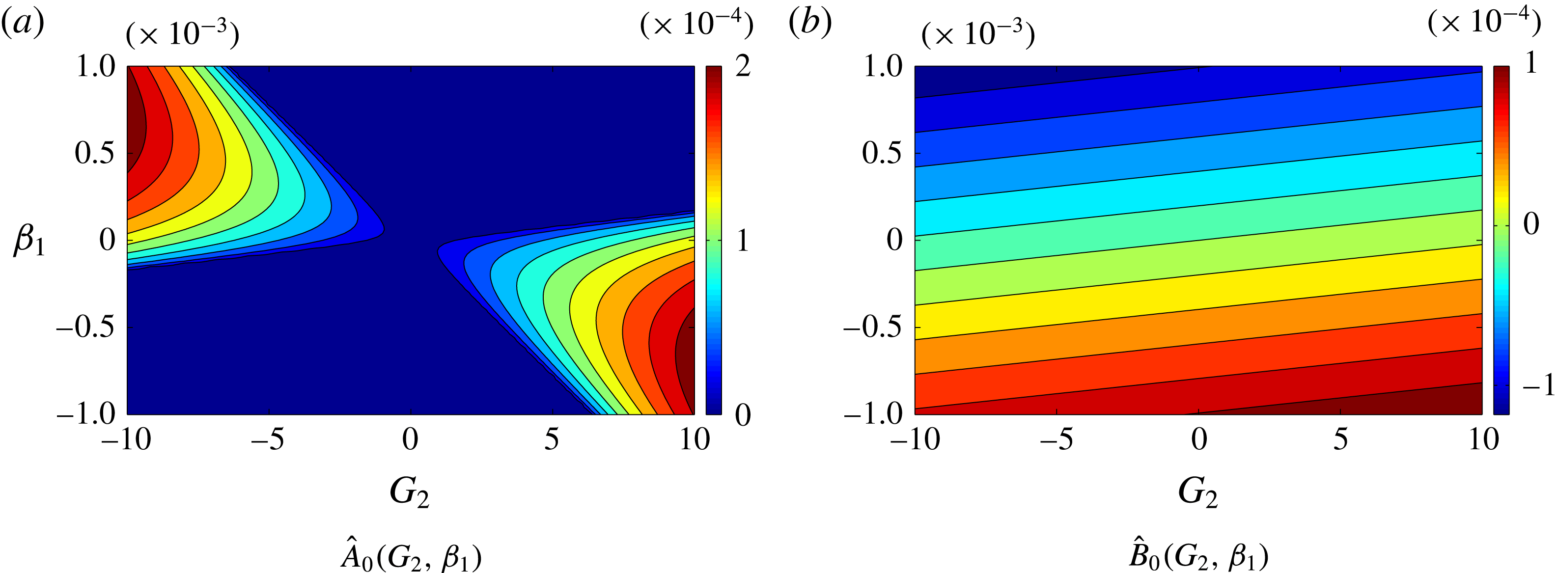
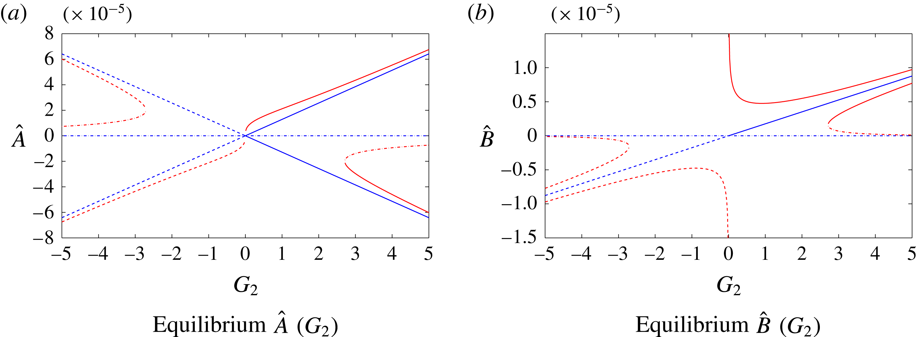
which exist provided the argument of the square root is positive. Thus solutions in the $G_{2}-\unicode[STIX]{x1D6FD}_{1}$ plane exist between the straight lines with gradients $-b_{2}/b_{1}$ and $-a_{2}/a_{1}$ . This can be seen from the plots of $\hat{A}_{0}$ and $\hat{B}_{0}$ in figure 3 which have been computed using the appropriate values of $a_{1},a_{2}$ etc.

Figure 3.

Contours of constant values of $\hat{A}_{0}$ and $\hat{B}_{0}$ for varying $G_{2}$ and $\unicode[STIX]{x1D6FD}_{1}$ .

3.4 Computation of fully nonlinear Görtler vortices

In this section we consider (3.6) once again but now look for fully nonlinear solutions computationally using a spectral method. Once again the domain was truncated in the wall-normal direction at some large distance $H$ from the wall, and then mapped linearly onto $[-1,1]$ , where we will use $\unicode[STIX]{x1D70C}$ to denote the new bounded and scaled wall-normal coordinate. The truncation height $H$ is increased until the results are independent of the chosen truncation height. A Chebyshev/Fourier basis was applied with the collocation/Galerkin method in the wall-normal/spanwise direction, where we denote the $n$ th Chebyshev polynomial by $T_{n}$ . Dealing with a semi-infinite domain using Chebyshev polynomials in this way was investigated by Boyd (Reference Boyd1982) who found that this method is satisfactory provided the solution is analytic, which we expect it to be. We can exploit symmetries in the governing equations to write the solutions in the form of the series expansions,

which are truncated at suitably large $(n,k)=(N,K)$ determined by requiring sufficient decay in the spectral coefficients, typically to approximately $10^{-8}$ . The resulting equations for $\bar{u}_{n,k}$ and $\unicode[STIX]{x1D713}_{n,k}$ are nonlinear, and are thus solved using the Newton method. Starting off the Newton iteration requires a good initial guess to stop the solution being attracted to the zero solution $\bar{u}_{n,k}=\unicode[STIX]{x1D713}_{n,k}=0$ for all $n,k$ . There are multiple ways to get around this issue such as using the predictions of the weakly nonlinear analysis as starting guesses, but here we used a random initial guess (with some sensible restrictions) to find a single solution. Once we have one solution, it is possible to generate all other solutions which bifurcate from the first mode linear neutral point by tracking the solution in the Görtler number $G$ as we did here, but solutions could also be tracked in spanwise wavenumber $\unicode[STIX]{x1D6FD}$ or some measure of the amplitude of the state such as the infinity norm $\Vert \bar{u}\Vert _{\infty }$ which will be used to visualise some of the bifurcations.

Figure 4.

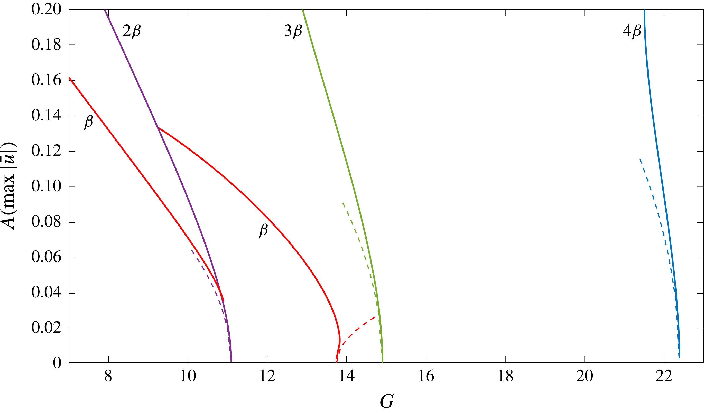
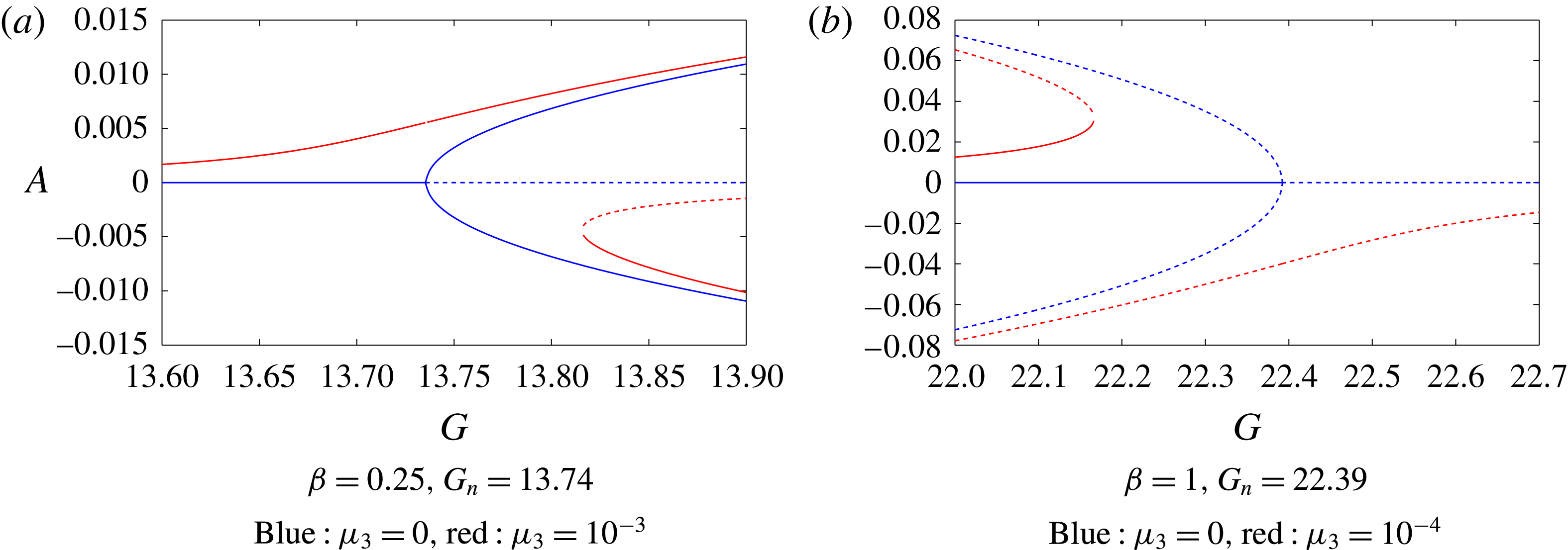
Bifurcation curves in $(G,A)$ space for spanwise wavenumbers $\unicode[STIX]{x1D6FD},2\unicode[STIX]{x1D6FD},3\unicode[STIX]{x1D6FD}$ and $4\unicode[STIX]{x1D6FD}$ as labelled, where $\unicode[STIX]{x1D6FD}=0.25$ . The solid lines represent bifurcation curves calculated from the nonlinear equations (3.6) and the dashed lines are the corresponding weakly nonlinear analysis from (3.10).

Figure 4 shows the equilibrium curves for the case when the spanwise wavenumber $\unicode[STIX]{x1D6FD}=0.25$ . In addition to the result shown in red for the finite amplitude state with wavenumber $\unicode[STIX]{x1D6FD}$ bifurcating from the unperturbed state we have also shown results in purple, green and blue the equilibrium states for the wavenumbers $2\unicode[STIX]{x1D6FD},3\unicode[STIX]{x1D6FD}$ and $4\unicode[STIX]{x1D6FD}$ respectively bifurcating from the unperturbed state. The dotted curves shown near the bifurcation points correspond to our weakly nonlinear predictions of the initial forms of the bifurcating solutions; we note the excellent agreement between the small and finite amplitude predictions near the bifurcation point. As anticipated by the weakly nonlinear theory only the equilibrium state corresponding to $\unicode[STIX]{x1D6FD}$ bifurcates supercritically at $G_{n}(\unicode[STIX]{x1D6FD})\approx 13.74$ and in fact at higher amplitudes a saddle-node bifurcation point is reached with the amplitude then increasing with decreasing $G$ . If this solution is then followed it meets the $2\unicode[STIX]{x1D6FD}$ solution as shown and so can be viewed as a supercritical subharmonic solution bifurcating from the $2\unicode[STIX]{x1D6FD}$ solution. At a smaller amplitude on the $2\unicode[STIX]{x1D6FD}$ solution there is a further subharmonic bifurcation to a solution with wavenumber $\unicode[STIX]{x1D6FD}$ but in this case the bifurcation is subcritical.

The bifurcations for the wavenumbers $2\unicode[STIX]{x1D6FD},3\unicode[STIX]{x1D6FD}$ and $4\unicode[STIX]{x1D6FD}$ are subcritical and some of these branches have been tracked to turning points when $\max |\bar{u}|\approx 0.3$ , although as the amplitude increases the wall-normal size of the structures increases requiring an increase in the wall-normal truncation height $H$ and resolution adding computational cost. Thus we will not pursue solutions to amplitudes larger than those shown in figure 4 of $\max |\bar{u}|\approx 0.2$ . As already noted above the $2\unicode[STIX]{x1D6FD}$ branch bifurcates from its linear neutral point $G_{n}(2\unicode[STIX]{x1D6FD})\approx 11$ and soon after, at a fairly small amplitude, there is a secondary bifurcation of a branch with spanwise wavenumber $\unicode[STIX]{x1D6FD}$ from the $2\unicode[STIX]{x1D6FD}$ branch, after which both branches continue to larger amplitudes. The $3\unicode[STIX]{x1D6FD}$ and $4\unicode[STIX]{x1D6FD}$ branches bifurcate from their respective linear neutral points, and continue into larger amplitudes. It is possible to test for bifurcations from the equilibrium solutions by monitoring the Jacobian used in our Newton iteration procedure. We conclude that the solutions shown in figure 4 have no other secondary bifurcations to modes with wavenumber $\unicode[STIX]{x1D6FD}$ or higher. However, this does not rule out the possibility of subharmonic bifurcations of i.e. spanwise wavenumber $\unicode[STIX]{x1D6FD}/2$ which could not be picked up in this computation because the numerical method looks for solutions which are periodic in a spanwise box of size $2\unicode[STIX]{x03C0}/\unicode[STIX]{x1D6FD}$ . General subharmonics would be difficult to find using the numerical method applied so far, so we concentrate only on the first subharmonic by replacing $\unicode[STIX]{x1D6FD}$ by $\unicode[STIX]{x1D6FD}/2$ in the computations. There is no reason to think that we have picked a special wavenumber here, in fact the situation should be generic provided the spanwise wavenumber is not changed by too much.

In order to see how the $\unicode[STIX]{x1D6FD}/2$ subharmonic can come into play we will consider the spanwise wavenumber $0.295$ , but to allow for the possibility of picking up the first subharmonic we alter the spanwise wavenumber so that $2\unicode[STIX]{x1D6FD}=0.295$ , i.e.  $\unicode[STIX]{x1D6FD}=0.1475$ . For the purpose of comparing the results with figure 4, we let $\unicode[STIX]{x1D6FD}^{\star }=2\unicode[STIX]{x1D6FD}$ . 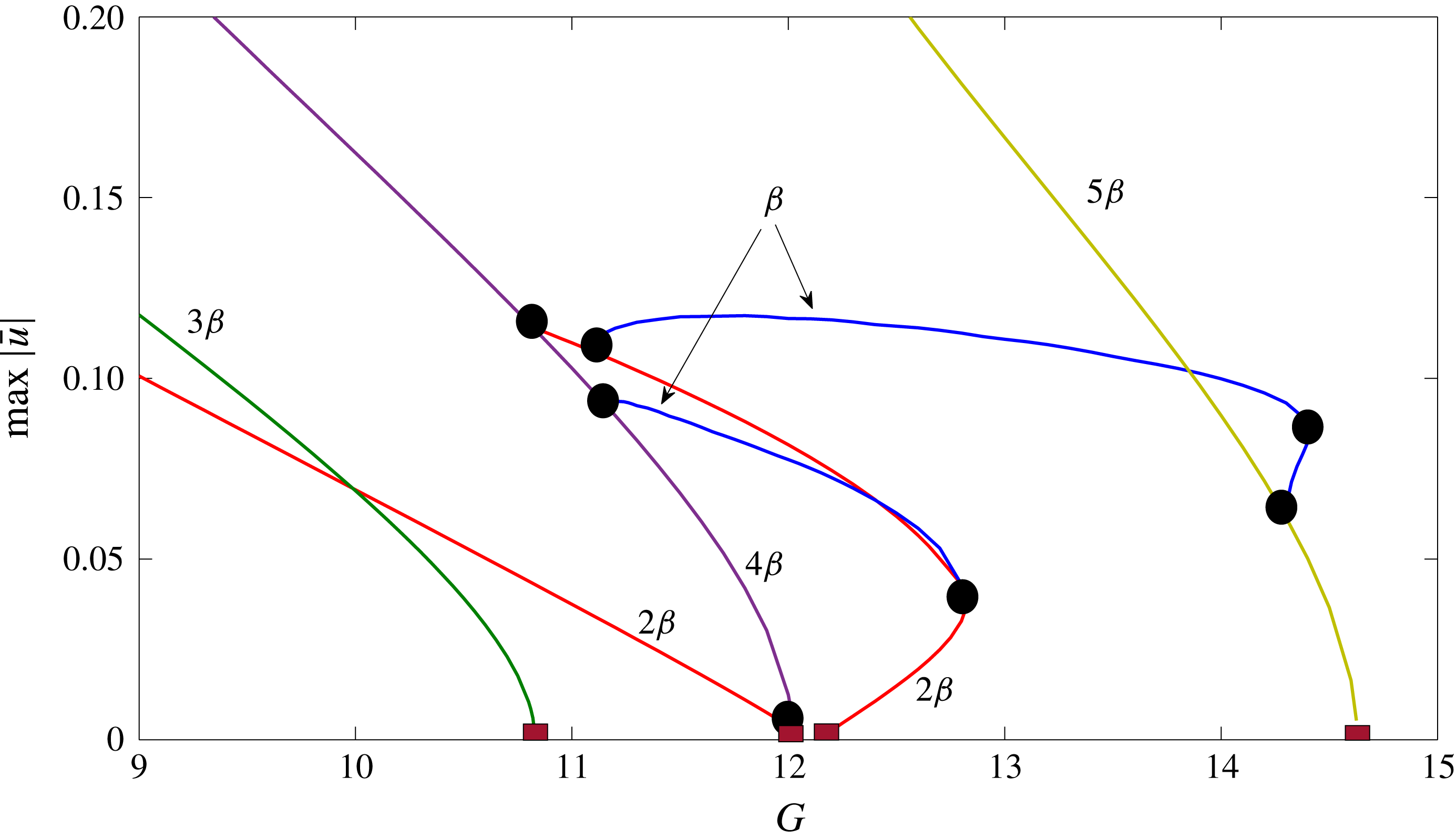The results of this computation can be seen in figure 5. In this figure we have denoted the linear neutral points by brown squares, and the secondary and saddle-node bifurcations by black circles for clarity. Taking only the $2\unicode[STIX]{x1D6FD}$ and $4\unicode[STIX]{x1D6FD}$ branches ( $\unicode[STIX]{x1D6FD}^{\star }$ and $2\unicode[STIX]{x1D6FD}^{\star }$ branches) into consideration for a moment, we see a very similar bifurcation structure as in figure 4. However we find branches with spanwise wavenumber $\unicode[STIX]{x1D6FD}$ ( $\unicode[STIX]{x1D6FD}^{\star }/2$ ) connecting the $2\unicode[STIX]{x1D6FD}$ and $4\unicode[STIX]{x1D6FD}$ ( $\unicode[STIX]{x1D6FD}^{\star }$ and $2\unicode[STIX]{x1D6FD}^{\star }$ ) branches, and also the $2\unicode[STIX]{x1D6FD}$ and $5\unicode[STIX]{x1D6FD}$ ( $\unicode[STIX]{x1D6FD}^{\star }$ and $5\unicode[STIX]{x1D6FD}^{\star }/2$ ) branches.

Figure 5.

Bifurcation curves in $(G,A)$ space for spanwise wavenumbers $\unicode[STIX]{x1D6FD},2\unicode[STIX]{x1D6FD},3\unicode[STIX]{x1D6FD},4\unicode[STIX]{x1D6FD}$ and $5\unicode[STIX]{x1D6FD}$ as labelled, where $\unicode[STIX]{x1D6FD}=0.1475$ . The solid lines represent the bifurcation curves with different colours denoting different spanwise wavenumbers as labelled, for clarity. The brown squares denote the linear neutral points for spanwise wavenumbers $2\unicode[STIX]{x1D6FD},3\unicode[STIX]{x1D6FD},4\unicode[STIX]{x1D6FD}$ and $5\unicode[STIX]{x1D6FD}$ (the linear neutral point for spanwise wavenumber $\unicode[STIX]{x1D6FD}$ occurs at a much larger Görtler number). The black circles show the locations of the secondary bifurcations and saddle-node bifurcations (turning points).

The results of the weakly nonlinear theory and indeed the finite amplitude numerical calculations suggest that the Taylor–Görtler instability of asymptotic suction flow behaves quite differently from centrifugal instabilities in Couette flow or growing boundary layers. The key difference is obvious already in figure 1(a) which shows that the most dangerous mode of instability bifurcates subcritically from the unperturbed state rather than supercritically as has long been established for Couette flow. We are unaware of any experiments which can be compared to this rather surprising result. For the Görtler vortex problem in growing boundary layers there have been many fully nonlinear simulations of vortex growth based on the marching scheme given for the linear case by Hall (Reference Hall1983) and the nonlinear case by Hall (Reference Hall1988). As far as we are aware all calculations have described the linear growth and supercritical saturation of vortices with no suggestion of the subcritical behaviour which might be anticipated if the growing and parallel boundary layer problems behave in the same way in the nonlinear regime. That is of concern because in stability theory asymptotic suction flow is viewed as a stepping stone between developed flows and growing boundary layers. The key difference between the parallel and growing case is associated with the fact that, as first pointed out by Hall (Reference Hall1983), boundary layer growth renders the concept of a unique neutral curve or growth rate untenable except at high vortex wavenumbers. In the latter case Hall & Lakin (Reference Hall and Lakin1988) showed that small wavelength Görtler vortices bifurcate supercritically; that is consistent with the prediction of supercritical bifurcations on the right-hand branch of figure 1(a) for sufficiently large wavenumbers. However for a growing boundary layer the local spanwise wavenumber increases at the same rate as the boundary layer growth so whatever the behaviour at a given value of the wavenumber we know that sufficiently far downstream the vortex will enter the Hall–Lakin regime and behave like a supercritical bifurcation. Presumably the many nonlinear simulations of Görtler vortices which have been carried out have been for initial wavenumbers sufficiently large that the vortices rapidly enter the Hall–Lakin regime.

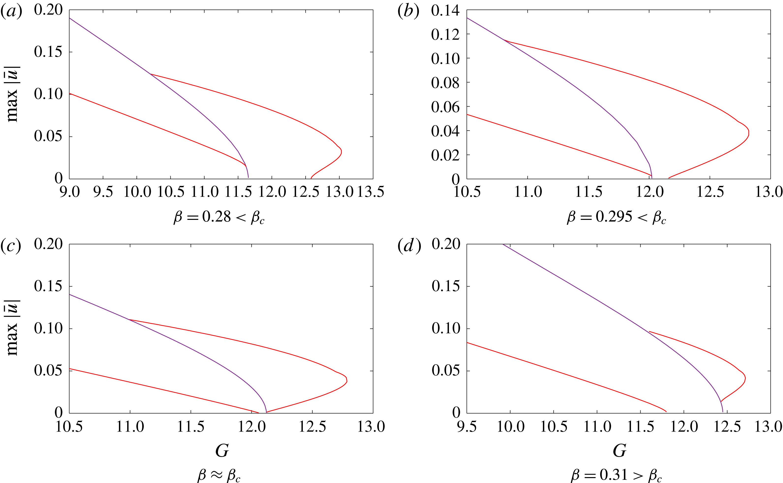
In § 3.3 we investigated how the bifurcation behaves around the resonant spanwise wavenumber $\unicode[STIX]{x1D6FD}\,=\,\unicode[STIX]{x1D6FD}_{c}$ , where the bifurcation changes from being supercritical to subcritical. To illustrate this in figure 6 we plot the bifurcation curves for $\unicode[STIX]{x1D6FD}$ and $2\unicode[STIX]{x1D6FD}$ for $\unicode[STIX]{x1D6FD}=0.28,\unicode[STIX]{x1D6FD}=0.295,\unicode[STIX]{x1D6FD}\approx \unicode[STIX]{x1D6FD}_{c}$ and $\unicode[STIX]{x1D6FD}=0.31$ in (a), (b), (c) and (d) respectively. In figure 6(a,b) where $\unicode[STIX]{x1D6FD}<\unicode[STIX]{x1D6FD}_{c}$ we see that as well as bifurcating from the unperturbed state the $\unicode[STIX]{x1D6FD}$ branch also arises as a secondary subharmonic bifurcation, one subcritical and the other supercritical, from the $2\unicode[STIX]{x1D6FD}$ branch at two points on the $2\unicode[STIX]{x1D6FD}$ curve. Note that in $(d)$ the $\unicode[STIX]{x1D6FD}$ branch bifurcating from the unperturbed state bifurcates supercritically but rapidly reaches a saddle-node point so that on the scale plotted, the bifurcation appears subcritical. Note however that the subharmonic bifurcations from the $2\unicode[STIX]{x1D6FD}$ curve are now both supercritical. A detailed examination in the neighbourhood of the case when $\unicode[STIX]{x1D6FD}=\unicode[STIX]{x1D6FD}_{c}$ produces results consistent with the weakly nonlinear theory.

Figure 6.

Bifurcation curves for $\unicode[STIX]{x1D6FD}$ (red) and $2\unicode[STIX]{x1D6FD}$ (purple) modes only, highlighting the change in behaviour as $\unicode[STIX]{x1D6FD}$ crosses $\unicode[STIX]{x1D6FD}_{c}$ for nonlinear equilibrium states computed from (3.6).

Given the number of bifurcations in figures 4–6 it is natural to ask if we have captured all the secondary bifurcations. Certainly we can be sure we have captured all of the primary bifurcations because of the analysis we performed in § 3.1. We could perform a linear stability analysis of each solution but in fact the numerical method applied here gives a much easier way to check for secondary bifurcations. Our method applied with a spanwise wavenumber $\unicode[STIX]{x1D6FD}$ looks for solutions to the governing equations (3.6) which are periodic in a spanwise box of length $2\unicode[STIX]{x03C0}/\unicode[STIX]{x1D6FD}$ . Provided any other solution is periodic in this box, it could also potentially be picked up using this numerical method and thus at any secondary bifurcation point the Jacobian in the Newton method must vanish. Thus, to check for secondary bifurcations with spanwise wavenumber $\unicode[STIX]{x1D6FD}$ or any higher harmonic thereof, we only need to monitor for example, the condition number of the Jacobian. This was the method used to find the location of the bifurcation curves, and then initialising the Newton method with the (suitable scaled) eigenfunctions of the Jacobian yields the new branches. Evidently, this method will not indicate when there are subharmonic bifurcations, but as alluded to before we expect that further subharmonic branches (i.e.  $\unicode[STIX]{x1D6FD}/4$ , etc.) are present in the state space.

4.1 Production layer analysis

In the first instance we review the free stream coherent structures found by DH. The only difference between the derivation given here and the work of DH is that in the absence of curvature an exact solution can be found for the basic state, whereas here with curvature present we must work with the leading-order approximation to the basic state. Thus for example the pressure is $-Re^{-2}Gy$   $+$  higher-order terms, but in fact this difference does not affect the leading-order analysis. The free stream coherent structures consist of a travelling wave state propagating in the streamwise direction at close to the free stream velocity. Activity is concentrated in two regions, the first of which is the subject of this subsection, and the second will be the subject of the next subsection. Firstly, we describe the nonlinear layer where the free stream structures are generated; this is of $O(1)$ extent and sits in the free stream a large distance, denoted by $\unicode[STIX]{x1D705}(Re)$ , from the wall. The majority of this subsection will be devoted to an examination of this layer. We will discuss the scales over which the interaction occurs, and the distance $\unicode[STIX]{x1D705}$ at which the layer sits from the wall. Coming out of this layer towards the wall, the streamwise velocity is growing exponentially. This growth continues until the second region of increased activity is reached, which is another layer of $O(1)$ extent but this time located near the wall where the velocity must adjust to satisfy the boundary conditions on the wall. Due to the nonlinear interaction in the layer in the free stream, the flow which the wall layer sees in the free stream is some perturbation to the basic state, and this drives near-wall structures.

Figure 7.

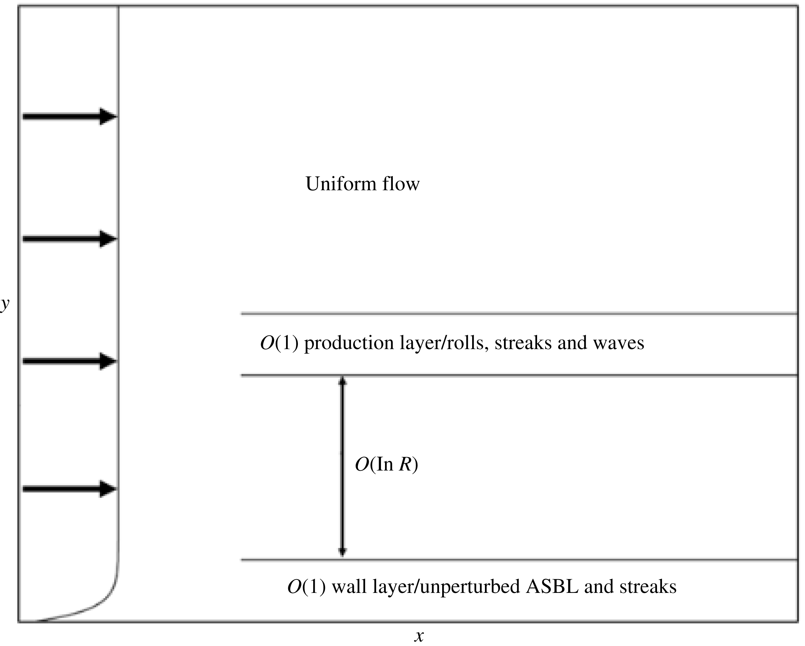
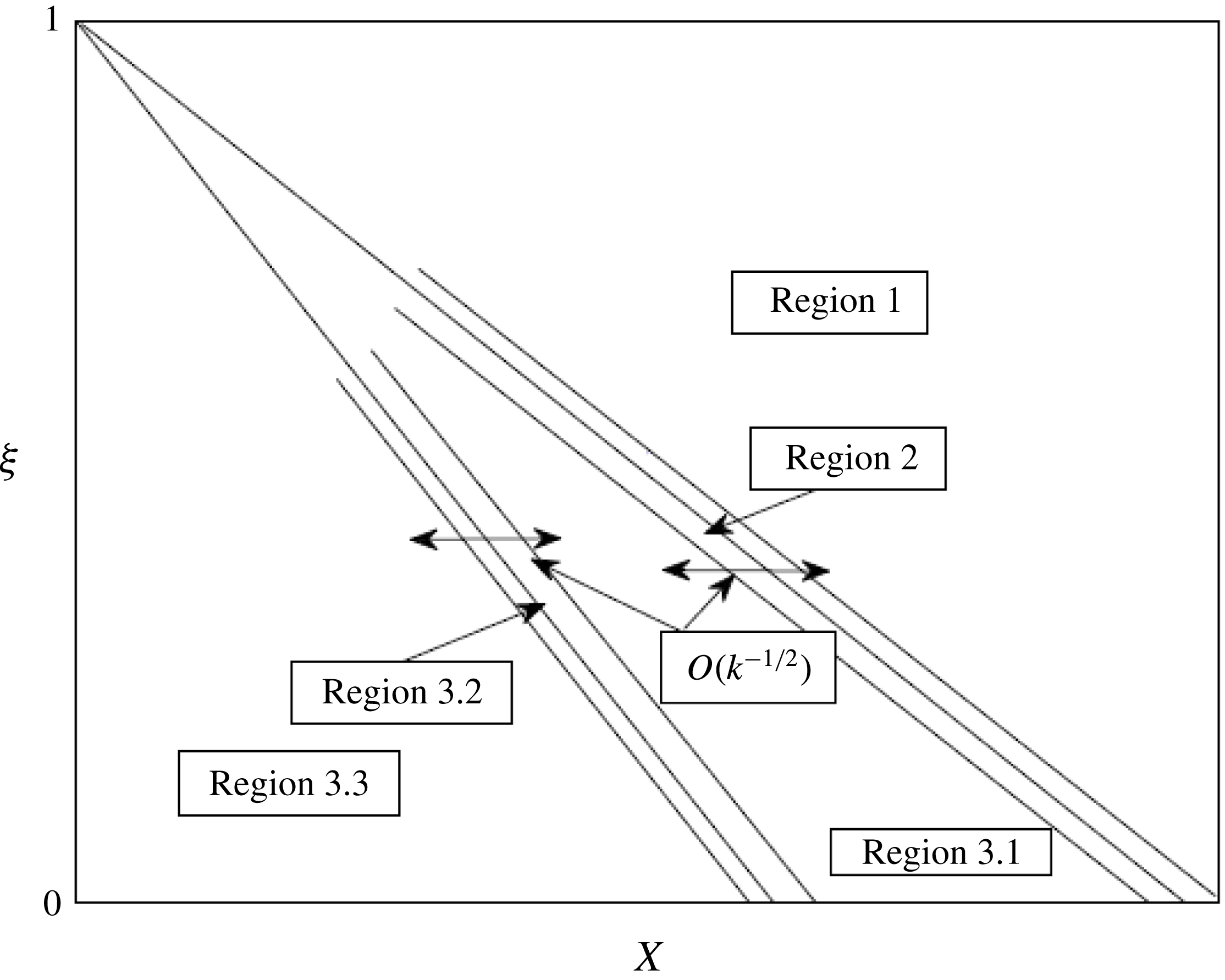
Schematic of the different regions associated with the free stream coherent structures of DH. The production layer is where the nonlinear interaction takes place and it produces a streaky flow growing exponentially towards the wall.

Now let us concentrate on the first region which DH refer to as the production layer. Here the nonlinear interaction driving a free stream coherent structure occurs. We are interested in a nonlinear travelling wave structure where all length scales involved in the interaction are comparable, in this case we assume they are all $O(1)$ . Then for a viscous–inviscid balance $vu_{y}\sim wu_{z}\sim Re^{-1}u_{yy}$ so we require that $v,w\sim O(Re^{-1})$ . Then from a wall-normal pressure balance $p_{y}\sim Re^{-1}v_{yy}$ we find that $p\sim O(Re^{-2})$ . As this structure sits in the free stream we know that $u\sim 1$ , and in fact the continuity equation $u_{x}\sim v_{y}$ yields $u-1\sim O(Re^{-1})$ . The streamwise advection term $\unicode[STIX]{x2202}_{t}+u\unicode[STIX]{x2202}_{x}$ written in a travelling wave coordinate $X=x-ct$ is $(u-c)u_{X}$ . Since the streamwise momentum equation is at $O(Re^{-1})$ , then in order to have a non-trivial interaction we require $u-c\sim O(Re^{-1})$ and thus for the wavespeed $c$ to be close to the free stream velocity, $c-1\sim O(Re^{-1})$ . Since $u$ must include the basic state $1-\text{e}^{-y}$ it follows that the production layer must be located where $\text{e}^{-y}\sim Re^{-1}$ , which happens when $y\sim \ln Re$ . Given that flow in the production layer has velocities of size $O(Re^{-1})$ and varies on an $O(1)$ length scale in all three directions it is easy to show that it must be located a distance $\unicode[STIX]{x1D705}=\ln Re$ from the wall. The different regions of interest are sketched in figure 7. Therefore we define the wall-normal production layer coordinate, $Y$ , defined by $Y=y-\ln (Re)$ . Motivated by the above scaling argument we let $c=1-Re^{-1}c_{1}$ and write

The variables $(U,V,W,P)$ depend on $(X,Y,z)$ where $X$ is the travelling wave coordinate $X=x-ct$ . The governing equations in the production layer are found to be the full Navier–Stokes equations with Reynolds number equal to unity in a streamwise travelling frame,

where $\unicode[STIX]{x1D735}_{1}=(\unicode[STIX]{x2202}_{X},\unicode[STIX]{x2202}_{Y},\unicode[STIX]{x2202}_{z})$ , and we have the far-field matching conditions,

Equations (4.2) govern the strongly nonlinear interaction of a wave travelling in the streamwise direction and a vortex flow inside the production layer. We note that curvature has no effect in the production layer at leading order, and thus these are exactly the equations considered by DH. In other words, the form of the production layer forcing on the flow below is the same at leading order whether curvature is present or not. We consider the effect of the production layer on the structures below, noting that the boundary conditions (4.2c ) allow for exponential growth of the streak provided it is not as fast as $\text{e}^{-Y}$ . We linearise in the far field below the production layer as $Y\rightarrow -\infty$ by setting

The wave is observed to decay below the production layer so the variables only depend on $Y$ and $z$ in the far field. Substituting (4.3a,b ) into (4.2) and linearising, the governing equations for the perturbations $(\hat{u} ,\hat{v})$ are found to be

There are solutions of these equations of the form $\hat{u} \propto \text{e}^{(\unicode[STIX]{x1D714}-1)Y}$ and $\hat{v}\propto \text{e}^{\unicode[STIX]{x1D714}Y}$ , where $\unicode[STIX]{x1D714}$ satisfies $(\unicode[STIX]{x1D714}^{2}+\unicode[STIX]{x1D714}-\unicode[STIX]{x1D6FD}^{2})(\unicode[STIX]{x1D714}^{2}-\unicode[STIX]{x1D6FD}^{2})=0$ . The boundary conditions (4.2c ) confine $\unicode[STIX]{x1D714}$ to lie in the interval $(0,1)$ , i.e. the streak must grow approaching the wall but no faster than $\text{e}^{-Y}$ . In fact we find that

The decaying exponential $\text{e}^{\unicode[STIX]{x1D714}Y}$ dominates the roll solution moving down away from the production layer and its interaction with the mean flow can produce an exponentially growing streak. That growth requires $0<\unicode[STIX]{x1D714}<1$ , so we see from (4.5) that this argument is only valid provided $0<|\unicode[STIX]{x1D6FD}|<\sqrt{2}$ . The relevant far-field behaviour is then found to be

where $J$ and $K$ are constants, related by the condition $K=-2\unicode[STIX]{x1D714}J$ . The constant $J$ depends on both the streamwise and spanwise wavenumbers of the nonlinear interaction inside the production layer, and can only be determined by solving the relevant (4.2) which must be done computationally, but for the purposes of this work it is enough to know that solutions to this set of equations do exist as demonstrated in the work of DH. The reader is referred to DH for more details of $J$ and $K$ . Also we observe that since $\hat{u}$ grows at a rate proportional to $\text{e}^{-Y}$ relative to $\hat{v}$ in the direction of the wall and the production layer is a distance $\ln Re$ from the wall the streak and roll parts of the flow adjust to being in the ratio $Re:1$ appropriate to a Görtler vortex structure in the unperturbed boundary layer. Thus, noting that $\text{e}^{\unicode[STIX]{x1D714}Y}=Re^{-1}\text{e}^{\unicode[STIX]{x1D714}y}$ , we conclude that the matching the velocity field in the wall layer to streamwise vortex structure induced beneath the production layer requires

where $\unicode[STIX]{x1D6FF}=Re^{-\unicode[STIX]{x1D714}}$ . The normal velocity component above is exponentially decreasing towards the wall whereas the roll part of a Görtler vortex would decay away from the wall and so a solution of the Görtler equations driven by (4.6) can be readily found. However when the unforced problem has a solution the forcing will cause the instability to occur as an imperfect bifurcation. The mechanism is thus essentially identical to that discussed by Hall & Walton (Reference Hall and Walton1977) in the context of Bénard convection forced by end walls or boundary imperfections. No further analysis of the production layer is required for this work, and in fact the rest of this paper will focus on the excitation of Görtler vortices by the free stream coherent structures which are felt through the matching condition (4.7) which acts as a forcing term on the near-wall problem in § 3.2.

In the context of receptivity theory (4.6) is highly significant. Receptivity theory relates the amplitude of an instability generated by some forcing to the amplitude of the forcing. Here we have so far considered only the equilibrium case where the forcing occurs over all $x$ and the next section will address the initial value version of the theory. However (4.6) tells us immediately that tiny waves, rolls and streaks of size $O(Re^{-1})$ interacting in the production layer induce a streak of size $O(Re^{-\unicode[STIX]{x1D714}})$ in the wall layer. 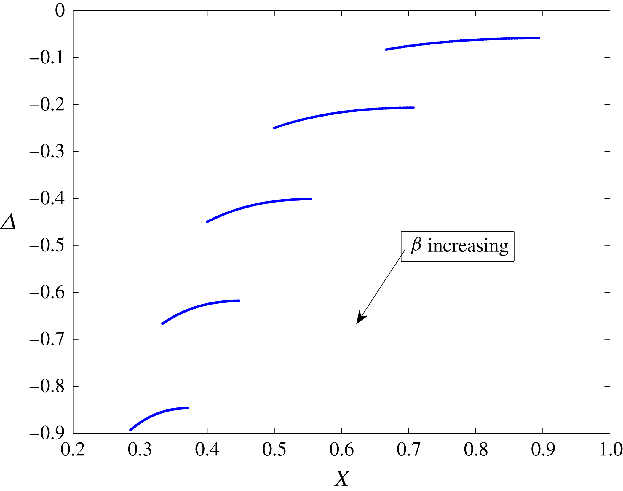In other words, using the definition of $\unicode[STIX]{x1D714}$ the streak induced by the forcing in the production layer has been amplified in magnitude by a factor $Re^{3-\sqrt{1+4\unicode[STIX]{x1D6FD}^{2}}/2}$ . The formal analysis of DH shows that streaks only grow if $\unicode[STIX]{x1D6FD}$ is in the range $(0,\sqrt{2})$ so that in the limiting case $\unicode[STIX]{x1D6FD}\rightarrow 0$ the induced streak would be comparable with the unperturbed flow. However numerical solutions of the production layer problem are so far limited to the case considered by DH and Deguchi & Hall (Reference Deguchi and Hall2015). For that case in the production layer the flow is periodic in the spanwise direction with wavenumber $\unicode[STIX]{x1D6FD}/2$ , however the response beneath the layer is subharmonic and so the flow there has spanwise wavenumber $\unicode[STIX]{x1D6FD}$ . The computation has been done when the streamwise and spanwise wavenumbers of production layer are in the ratio $1/2$ and in that case Deguchi & Hall (Reference Deguchi and Hall2015) found eigenvalues for $\unicode[STIX]{x1D6FD}$ in the approximate range $(0.41,0.93)$ . Taking the lowest value of $\unicode[STIX]{x1D6FD}$ we see then that the induced streak in the wall is bigger by a factor of approximately $Re^{.85}$ than the disturbance in the production layer which generates it. This remarkable increase in the induced amplitude compared to the smaller velocities in the production layer is surprising and goes through to § 5 where we consider the spatial initialisation process for the structure.

4.2 Wall layer analysis

As discussed in the previous subsection, the presence of the production layer causes structures to develop near the wall where the flow must adjust to satisfy the no-slip boundary conditions on the wall. Recalling the results of § 3.2, we saw the formation of near-wall structures in the absence of the production layer and these were caused purely by wall curvature. In this subsection we will see how the structures observed within the wall layer in § 3.2 are affected by the presence of free stream coherent structures. If we now consider the flow near the wall where $y\sim O(1)$ , then the governing equations (3.6) are altered by the far-field matching condition inherited from the production layer via (4.7), so that the far-field matching in the governing equation (3.6c,d ) is replaced by

There are four different regimes to consider here depending on the value of the spanwise wavenumber and the Görtler number $G$ . First for a general $\unicode[STIX]{x1D6FD}$ , there are three different regimes to consider depending on whether the Görtler number is less than, close to, or greater than the neutral Görtler number. When the Görtler number is less than the neutral Görtler number the solution is of the form

from which we find the governing equations are (3.6) but with the far-field matching conditions in (3.6c,d ) replaced by $\widehat{U}\sim J\text{e}^{(\unicode[STIX]{x1D714}-1)y}$ and $\widehat{\unicode[STIX]{x1D6F9}}\sim \unicode[STIX]{x1D6FD}^{-1}K\text{e}^{\unicode[STIX]{x1D714}y}$ as $y\rightarrow \infty$ . The governing equations are linear, and we see overall that the $O(\unicode[STIX]{x1D6FF})$ forcing from the production layer results in near-wall structures with size $O(\unicode[STIX]{x1D6FF})$ . As the Görtler number approaches the neutral Görtler number, the problem becomes degenerate and the solution grows like $(G-G_{n})^{-1}$ so that the solution breaks down for $G\sim G_{n}$ which is the second regime and will be discussed in more detail shortly. The third regime is when the Görtler number is larger than the neutral Görtler number. In this case the basic state is linearly unstable and we would expect to see a fully nonlinear state of the type seen in § 3.4. For the final regime recall in § 3.3, that there is a special value of the spanwise wavenumber denoted by $\unicode[STIX]{x1D6FD}_{c}$ where we find both the first and second harmonics are present at leading order and in this scenario the bifurcation structure is altered. This will be discussed later in the this section.

First we will discuss the second regime. Recalling the analysis without a production layer in § 3.2 we assume the leading-order solution is $O(\unicode[STIX]{x1D716})$ and following the arguments of § 3.2 we pose the expansion (3.8) with $\unicode[STIX]{x1D716}(\unicode[STIX]{x1D6FF})$ to be determined. Now because $G\sim G_{n}$ , the leading-order problem is degenerate and thus the forcing, which is on the first harmonic, must be applied at $O(\unicode[STIX]{x1D716}^{3})$ . So we conclude that the relevant expansion in this regime is (3.8) with $\unicode[STIX]{x1D716}=\unicode[STIX]{x1D6FF}^{1/3}$ . The analysis at $O(\unicode[STIX]{x1D716})$ and $O(\unicode[STIX]{x1D716}^{2})$ is identical to that of § 3.2 and so (3.10), (3.11) once again apply. The conditions at the wall remain unchanged but the forcing from the streak generated in the production layer requires that at $O(\unicode[STIX]{x1D716}^{3})$ we now have a new far-field matching condition of the form

which represents the forcing on the near-wall flow by the production layer. The forcing term above corresponds to one of the exponentially increasing (away from the wall) solutions of the (3.11) with ${U_{1}}^{(3)}=0.$ In order to convert this condition into a form where we can apply the adjoint condition we let $U^{p},\unicode[STIX]{x1D6F9}^{p}$ be the solution of the homogeneous form of (3.11) which at infinity satisfies (4.9) with no contributions from the other three decaying solutions of the sixth-order form of the homogeneous equations. Without those other solutions the conditions at the wall cannot be satisfied and so the problem for $U_{1}^{(3)},\unicode[STIX]{x1D6F9}_{1}^{(3)}$ is equivalent to solving (3.11) written as a sixth-order system with $\boldsymbol{Z}\rightarrow 0,y\rightarrow \infty$ and

This inhomogeneous wall condition is independent of the amplitude but will contribute to the solvability condition through the concomitant. The amplitude (3.12) is therefore found to be replaced by

where $\unicode[STIX]{x1D707}_{0},\unicode[STIX]{x1D707}_{1}$ and $\unicode[STIX]{x1D707}_{2}$ are identical to the corresponding constants in (3.9) and $\unicode[STIX]{x1D707}_{3}$ is a constant proportional to $J$ . Thus equilibrium states are now found to satisfy the equation

Provided there is forcing of the streak from the production layer ( $J\neq 0$ ), it is possible to scale $\unicode[STIX]{x1D707}_{3}$ out of the problem, which comes from the solution of the production layer problem, by setting

and then the amplitude equation becomes

This demonstrates that the effect of changing the level of production layer forcing is simply a rescaling of the variables, although for our illustrations we will use (4.13).

Figure 8.

Bifurcation diagram showing $A(G)$ . The blue curve shows the perfect bifurcation when $J=0$ , and the red curve shows the imperfect bifurcation when $J\neq 0$ . Stable branches are solid curves, and unstable branches are dashed curves.

Figure 8 shows plots in $(G,A)$ space for two different values of the spanwise wavenumber, $\unicode[STIX]{x1D6FD}=0.25$ and $\unicode[STIX]{x1D6FD}=1$ as used before in figure 4. For each spanwise wavenumber we see the bifurcation curve with no free stream coherent structures, $J=0$ , and in the presence of free stream coherent structures, where $J\neq 0$ (values given in the captions). The blue curves for $J=0$ are identical to the curves in figure 4, but by setting $J\neq 0$ given by the red curves we see how breaking the symmetry creates an imperfect bifurcation. In figure 8 we have used line style to denote the stability of each branch, applying the normal convention of solid curves for stable states and dashed curves for unstable states. First we will discuss the $\unicode[STIX]{x1D6FD}=0.25$ case. For $J=0$ , the perfect bifurcation is supercritical and we have one stable branch bifurcating into one unstable branch and a pair of stable branches. When $J\neq 0$ the bifurcation is imperfect and there are now two disconnected curves. One is a stable branch, then there is also a saddle-node bifurcation into a stable–unstable pair at a particular value of $G\simeq 13.82$ . Note that the location of this bifurcation has moved between $J=0$ and $J\neq 0$ , and in the future we will denote the location of the bifurcation in the $J\neq 0$ case by $G_{b}$ , so for example in this case we have $G_{b}\approx 13.82$ . Now consider the $\unicode[STIX]{x1D6FD}=1$ case. For $J=0$ , the perfect bifurcation is subcritical consisting of a bifurcation of one stable and an unstable pair of branches into a single unstable branch. When $J\neq 0$ the bifurcation is imperfect and once again this becomes two disconnected curves one of which is an unstable branch and the other is a stable–unstable pair which terminate at some value of $G$ denoted as before by $G_{b}\approx 22.17$ . The results of figure 6(a) show that when the spanwise wavenumber is associated with a supercritical bifurcation the Taylor–Görtler vortex in the wall layer is always stable to disturbances with the same wavenumber and that as the Görtler number increases through the linear critical the vortex has its size increased until for large $G_{1}$ the leading-order approximation to the vortex amplitude is independent of the size of the forcing from the production layer. In fact receptivity theory is a concept perhaps most easily understood within the context of linear theory. Usually the main issue is what is the size of a linearly growing disturbance induced by an external forcing mechanism. Therefore in order to derive receptivity coefficients it is more appropriate to consider the linear initial value problem for the case when the production layer forcing begins at some given value of $\overline{x}$ , that will be discussed in the next section. However we do note the rather remarkable result that the nonlinear self-sustaining interaction in the production layer involving rolls, waves and streaks induces a much larger finite amplitude Görtler vortex within the wall layer.

Now we will briefly discuss the fourth regime, when the spanwise wavenumber is close to the resonant spanwise wavenumber, similar to the analysis of § 3.3. Recalling the analysis of § 3.3 we assume a disturbance of size $O(\unicode[STIX]{x1D716})$ and are thus led to the expansion (3.13) with $\unicode[STIX]{x1D716}(\unicode[STIX]{x1D6FF})$ undetermined at this stage. The leading-order equations are degenerate and thus the forcing must appear at $O(\unicode[STIX]{x1D716}^{2})$ . Thus the relevant expansion is (3.13) with $\unicode[STIX]{x1D716}=\unicode[STIX]{x1D6FF}^{1/2}$ . The forcing only applies to the first harmonic, and hence only appears in the $\hat{A}$ evolution equation. Thus, following the analysis of § 3.3 which is unaltered at $O(\unicode[STIX]{x1D716})$ , we find the solvability condition (3.14) now becomes

where $G_{2}$ is defined by (3.15), the $a_{i},b_{i}$ for 1, 2, 3 are as in § 3.3, and $a_{4}$ is determined by the far-field behaviour of the adjoint zero eigenfunction which is used to find the solvability condition. In fact we could take the production layer streak forcing to be through the second harmonic streamwise wavenumber rather than the first harmonic. In that case $a_{4}=0$ and a term $b_{4}J$ is to be inserted in (4.15). The resulting solutions are qualitatively to those of (4.15) and so we restrict our attention to that case.

Figure 9 shows the equilibrium solutions of (4.16) for both perfect ( $J=0$ in blue) and imperfect ( $J\neq 0$ in red) bifurcations. The effect of the forcing from the production layer is to break the symmetry of the system and hence to create imperfect bifurcations as can clearly be seen in figure 9. Similarly to figure 8 we have denoted stable branches by solid curves and unstable branches by dashed curves. However, the system is a little more complicated now by the presence of two modes, and so there are also saddles which are marked as dot-dash curves.

Figure 9.

Perfect and imperfect bifurcations for near resonant $\unicode[STIX]{x1D6FD}$ . Here we have chosen $\unicode[STIX]{x1D6FD}_{1}=0$ so $\unicode[STIX]{x1D6FD}=\unicode[STIX]{x1D6FD}_{c}$ and have plotted the resulting bifurcations for $J=0$ (blue curve) and $J=10^{-4}$ (red curve). We have used line style to denote the stability of each branch with solid, dashed and dot-dashed for stable, unstable and unstable saddle respectively.

5.1 Adjustment layer analysis

Suppose that nonlinear solution in the production layer, located at $\unicode[STIX]{x1D705}=\ln Re$ , begins at say $\bar{x}=0$ . The boundary conditions at the top of the adjustment layer come from the production layer solution:

where ${\mathcal{H}}(\bar{x})$ denotes the Heaviside function and $\unicode[STIX]{x1D6FF}=Re^{-\unicode[STIX]{x1D714}}$ .

We will see below that the curvature has no effect on the leading-order velocity in the adjustment layer and is therefore of size $O(\unicode[STIX]{x1D6FF})$ there. In view of the above forcing it follows that $U,V,P$ defined in (2.3)–(2.4) must take the form

where $u_{s},v_{r},w_{r},p_{r}$ are functions of $\bar{x}$ and $y$ . In the previous section this led to the linearised problem, equations (3.4a–d ) but here we must consider spatial rather than temporal evolution. The governing equations for the linearised perturbations are

subject to the production layer forcing

This problem is posed for $\bar{x}>0$ and $y\in [0,\unicode[STIX]{x1D705}]$ , and it follows that the characteristic length scale in the wall-normal direction is $O(\unicode[STIX]{x1D705})$ . Since the boundary conditions imply that $u_{s},v_{r}\sim O(1)$ we see from the continuity equation that the characteristic streamwise length scale is also $O(\unicode[STIX]{x1D705})$ . We define adjustment layer variables $X$ and $\unicode[STIX]{x1D709}$ where

The governing equations in the adjustment layer (5.3) written in terms of adjustment layer variables are

subject to matching with the production layer forcing

where in the above $u_{b}$ denotes the basic flow written in $\unicode[STIX]{x1D709}$ coordinates but primes still denote differentiation with respect to $y$ , so for example $u_{b}=(1-\text{e}^{-\unicode[STIX]{x1D705}\unicode[STIX]{x1D709}})$ and $u_{b}^{\prime }=\text{e}^{-\unicode[STIX]{x1D705}\unicode[STIX]{x1D709}}$ . If $\unicode[STIX]{x1D709}\sim O(1)$ , then terms of the form $\text{e}^{-\unicode[STIX]{x1D705}(\cdot )}$ are exponentially small (when $(\cdot )$ is positive) and we find for example that $u_{b}\sim 1$ , and inspecting (5.5a ) it follows that $u_{s}\sim \text{e}^{-\unicode[STIX]{x1D705}\unicode[STIX]{x1D709}}v_{r}$ . Thus for $\unicode[STIX]{x1D709}\sim O(1)$ (5.5) become

subject to the boundary condition (5.5c,d ). Notice that the Görtler number $G$ is non-zero but curvature is a higher-order effect in the region where $\unicode[STIX]{x1D709}\sim O(1)$ , and in fact we find that it is only important at leading order within the wall layer, when $y\sim O(1)$ . Because $\unicode[STIX]{x1D705}$ is large, from the form of (5.6) and in particular the boundary conditions (5.5c,d ), we seek a WKB solution of the form

where $\hat{u}$ and $\hat{v}$ are amplitude functions and $\unicode[STIX]{x1D719}$ the WKB phase function are all functions of the slow variables $X$ and $\unicode[STIX]{x1D709}$ . The roll is decoupled from the streak in (5.6b ), so our strategy for solving the system is to solve for the roll first in (5.6b ) and then for the streak using (5.6a ). We simplify the analysis by first solving (5.6b ) for the vorticity $V_{r}$ defined by

From (5.6b ) we see that the governing equation for the vorticity $V_{r}$ is

and the far-field boundary condition (5.5c,d ) is

Seeking a WKB solution of (5.9) with phase $\unicode[STIX]{x1D703}$ and amplitude $\hat{V}$ , so $V_{r}=\hat{V}\text{e}^{\unicode[STIX]{x1D705}\unicode[STIX]{x1D703}}$ we find that the phase function $\unicode[STIX]{x1D703}$ satisfies

Solving this nonlinear equation using Charpit’s method we find the solution $\unicode[STIX]{x1D703}=\unicode[STIX]{x1D714}\unicode[STIX]{x1D709}$ for $\bar{\unicode[STIX]{x1D709}}(X)<\unicode[STIX]{x1D709}<1$ where

and this is the limiting characteristic emanating from the position where the production layer begins. This region is referred to as the upper adjustment layer and is identical to the parallel production layer problem considered by DH; it feels the production layer at $\unicode[STIX]{x1D709}=1$ but not the starting condition as $X=0$ i.e. the structure is fully developed (independent of $X$ ) in this region. However, here the vorticity must decay to zero as $X\rightarrow 0$ and thus we find that around $\unicode[STIX]{x1D709}\approx \bar{\unicode[STIX]{x1D709}}$ , there is a diffusion layer. The width of the diffusion layer is determined by balancing viscous and inviscid forces in the amplitude equation, from which it can be seen that the diffusion layer has thickness $\unicode[STIX]{x1D705}^{-1/2}$ – see Dempsey (Reference Dempsey2015) for more details. Below the diffusion layer, the vorticity is found to be exponentially small. We have now determined the vorticity throughout the whole of the adjustment layer. The vorticity is split into three distinct regions: region 1, the parallel region; region 2, the diffusive region; and region 3, the lower adjustment layer. Now that we have found the vorticity $V_{r}$ by solving (5.6b ), we can determine the roll $v_{r}$ by solving (5.8). Given the form of the vorticity, one might conclude that the roll is split into three regions, however the presence of a WKB turning point in the lower adjustment layer subdivides this region into three subregions, meaning there are five regions to consider in all: the parallel and diffusive regions from the vorticity discussion, plus three more regions from the lower adjustment layer which is now subdivided by a WKB turning point layer which is located at $\underset{\bar{\text{}}}{\unicode[STIX]{x1D709}}(X)$ where

and whose thickness is also determined to be of size $\unicode[STIX]{x1D705}^{-1/2}X^{1/2}$ by a viscous–inviscid balance of the WKB amplitude equation. Below the WKB turning point layer, in the fifth and final region, the flow is irrotational and the phase function for $v_{r}$ is no longer $\unicode[STIX]{x1D703}$ because of a switch in the dominant solution for the roll across the WKB diffusion layer. The discussion given in Dempsey (Reference Dempsey2015) shows that the WKB phase function $\unicode[STIX]{x1D719}$ is given by

The corresponding WKB phase for the streak is $\unicode[STIX]{x1D719}-\unicode[STIX]{x1D709}$ . Figure 11 shows plots of the WKB phases of the streak and roll for unit spanwise wavenumber, $\unicode[STIX]{x1D6FD}=1$ calculated using $\unicode[STIX]{x1D719}$ as given above. The black lines indicate the positions of the diffusion front (upper line) and the WKB turning point layer (lower line). From this figure, the WKB turning point layer appears to indicate the start of growth of the near-wall structures, and the diffusion layer marks the point where the structures become fully developed. The solution in the main part of the boundary layer will be driven by the WKB solution evaluated with $\unicode[STIX]{x1D709}=0$ . The response of the boundary layer to the forcing at the edge will depend on the Görtler number. If the forcing at any location stimulates a naturally occurring growing vortex then resonance will occur and we can relate the amplitude of the vortex to the amplitude of the forcing. In the more usual form of this kind of receptivity problem the amplitude of the forcing is arbitrarily small and the process is linear. Here the forcing is a function of the Reynolds number and so the possibility of nonlinear effects coming into play arises. However we do have the parameter $G$ at our disposal and our choice of $G$ will determine the linearity or otherwise of the process.

Now let us determine under what circumstances local resonance between the forcing and naturally occurring vortices can occur. At the top of the boundary layer the local growth rate with respect to $\bar{x}$ of the forced solution is to leading order $\unicode[STIX]{x1D719}_{X}(X,0)$ . This is of course $O(1)$ but varies slowly on the slow scale $X$ and if $\unicode[STIX]{x1D719}_{X}(X,0)$ somewhere coincides with the streamwise growth rate of an unstable Görtler vortex we expect that receptivity will occur. There is an important difference to note here concerning the ‘resonance’ conditions needed to induce an instability mode. In previous receptivity work the unperturbed boundary layer is spatially varying and so resonance occurs at a local position where the forcing and naturally occurring disturbance have coincident length and time scales. Here the boundary layer is parallel so the naturally occurring modes do not have their wavelength varying with the streamwise variable and so resonance occurs when locally the external agent, which is of course the free stream coherent structure, drives the boundary layer at its edge with the growth rate of a natural mode.

Figure 12 shows the typical dependence of $\unicode[STIX]{x1D719}_{X}(X,0)$ on $X$ , the results shown are for $\unicode[STIX]{x1D6FD}=0.2$ . We see that the growth rate is zero in the upper adjustment layer, has its constant maximum in region 3.1 and is monotonically decreasing between regions 3.1 and 1. Regions 3.1 and 3.2 are connected the WKB turning point layer of thickness $O(\unicode[STIX]{x1D705}^{-1/2})$ on the $X$ scale. Likewise the regions 3.1 and 1 connect through region 2 which is of similar width but the difference here is that the growth rate on the $\bar{x}$ scale has now fallen from being $O(1)$ to $O(\unicode[STIX]{x1D705}^{-1/2}).$ The region 2 is therefore a site of receptivity for weakly unstable vortices. Thus apart from regions 2 and 3.1 the forcing from the free stream will not induce a naturally occurring disturbance.

On the basis of figure 12 we can make some immediate observations. Suppose in the first instance that the spatial growth rate of a Görtler vortex for the given values of $\unicode[STIX]{x1D6FD},G$ is larger than the maximum value indicated in figure 10. In that case there is no streamwise location where the free stream forcing leads to a value of $\unicode[STIX]{x1D719}_{X}(X,0)$ as large as the growth rate and so no receptivity is possible. In other words the local growth of a forced vortex is always smaller than that of an unstable vortex and so the forced flow cannot resonate with the latter vortex. If the growth rate of an unstable vortex is lower than the maximum value of $\unicode[STIX]{x1D719}_{X}(X,0)$ shown in figure 12 then there will be a streamwise position where resonance occurs and a vortex will be induced. For $O(1)$ values of the growth rate then the forcing will induce a growing Görtler vortex in the neighbourhood of some location in region 3.1. If on the other hand the growth rate is small receptivity occurs close to the boundary of regions 1 and 3.1, since these regions are connected by the diffusion layer, i.e. region 2, receptivity will occur there. For $O(1)$ growth rates the induced Görtler vortex is growing too quickly for weakly nonlinear theory to come into play and so the regime discussed in the previous section does exist and the full nonlinear Görtler equations must be solved numerically as in Hall (Reference Hall1988). In the second case where the growth is small weakly nonlinear theory can apply but we show that surprisingly the receptivity analysis appropriate to that case predicts that the external forcing can initially only generate an algebraically growing form of the unstable mode which far downstream matches into the weakly nonlinear structure described in the previous section. In the absence of curvature or in the presence of convex curvature growing Görtler vortices are not possible and so there is no site of receptivity.

Figure 11.

WKB phase function for streaks ( $\unicode[STIX]{x1D719}-\unicode[STIX]{x1D709}$ , a) and rolls ( $\unicode[STIX]{x1D719}$ , b) in the adjustment layer for $\unicode[STIX]{x1D6FD}=1$ where $\unicode[STIX]{x1D719}$ is from (5.14). The black lines indicate the location of the diffusion layer $\overline{\unicode[STIX]{x1D709}}$ and the WKB turning point layer $\text{}\underline{\unicode[STIX]{x1D709}}$ .

Figure 12.

The growth rate $\unicode[STIX]{x1D719}_{X}$ with respect to $X$ of the forced flow at the edge of the boundary layer ( $\unicode[STIX]{x1D709}=0$ ) for $\unicode[STIX]{x1D6FD}=0.2$ .

5.2 Receptivity in the shadow region 3.1

It follows from the analysis in Dempsey (Reference Dempsey2015) that in the shadow region 3.1 the roll and streak velocities $v_{r},u_{s}$ defined by (5.2), (5.7) must at the edge of the unperturbed boundary layer satisfy

At any location $X$ we define a local spatial growth rate

which will to leading order coincide with the growth rate defined in terms of $u_{s}.$ The monotonically decreasing growth rate $\unicode[STIX]{x1D6F4}$ tends to a constant $\unicode[STIX]{x1D6F4}_{m}$ at $\text{}\underline{\unicode[STIX]{x1D709}}$ the beginning of the shadow region (3.1) and to zero where it ends in the diffusion layer. Note that in region 3.3 the corresponding growth rate is constant and equal to $\unicode[STIX]{x1D6F4}_{m}.$ Now suppose that for the given choice of $(G,\unicode[STIX]{x1D6FD})$ the linear stability problem specified by (5.3a,b ) with $u_{s},v_{r}\sim \text{e}^{\unicode[STIX]{x1D706}\overline{x}}$ subject to no slip at the wall and $u_{s},v_{r}$ vanishing at $\infty$ has an eigenvalue $\unicode[STIX]{x1D706}=\unicode[STIX]{x1D6F4}$ at some location $X_{L}$ . We define a new variable $\widehat{X}$ by

so that near $X_{L}$ the forcing at the edge of the boundary layer the roll must satisfy

and the streak satisfies

where

We now seek a solution of (5.3a,b ) in the neighbourhood of $X_{L}$ satisfying no slip at the wall together with the above condition for large $y.$ Because the homogeneous version of this problem has a solution $(\widehat{u}_{s}(y),\widehat{v}_{r}(y))$ we look for a solution $O(\unicode[STIX]{x1D705}^{1/2})$ larger than the above expressions and write

together with a similar expression for the streak. Here $B(\widehat{X})$ is an unknown amplitude. The leading-order problem is automatically satisfied because $(\widehat{u}_{s}(y),\widehat{v}_{r}(y))$ is a naturally occurring eigenfunction and at next order  we obtain an inhomogeneous version of the differential equations satisfied by the eigenfunction. In particular there will be terms proportional to $\text{d}B(\widehat{X})/\text{d}\widehat{X}$ in the differential equation together with terms proportional to $\exp (\unicode[STIX]{x1D6F4}^{\prime }(X_{L})\widehat{X}^{2})$ in the far-field boundary condition. The system will have a solution if the appropriate solvability condition is satisfied. That condition takes the form

where $d_{1}$ is a constant defined in terms of the leading-order eigenfunction and its adjoint. This is the crucial equation which fixes the receptivity coefficient. Noting that $\unicode[STIX]{x1D6F4}^{\prime }(X_{L})$ is negative the required solution of this equation matching with the upstream forcing in the absence of an incoming growing disturbance is

so that for large $\widehat{X}$

Here the first term represents the amplitude of the induced Görtler vortex and the exponentially decaying terms denoted by $\ldots$  match onto the forcing which persists for large $\widehat{X}$ . Of particular interest is the size of the induced vortex, apart from a constant this is the so-called receptivity coefficient. We deduce then that the induced vortex has amplitude of size $O(Re^{\unicode[STIX]{x1D6E5}})$ where

We note that the velocity field in the production layer which is responsible for the forcing is of size $Re^{-1}.$ Figure 13 shows $\unicode[STIX]{x1D6E5}$ for a range of values of the spanwise wavenumber $\unicode[STIX]{x1D6FD}$ as a function of position where the Görtler vortex problem has growth rate coincident with that of the free stream forcing. We see that in all cases the receptivity coefficient is a maximum at the end of the shadow region for the given value of $\unicode[STIX]{x1D6FD}$ . We also note that the receptivity coefficient increases monotonically with $\unicode[STIX]{x1D6FD}$ decreasing. Remarkably we observe that the production layer velocity field of size $Re^{-1}$ produces linearly growing vortices of much bigger amplitude. We also observe that at the end of the range where the receptivity coefficient exists the growth rate of the vortex approaches zero, thus we need to consider the case when the external forcing produces a growth rate appropriate to that in the diffusion layer. We shall now consider that case in detail and see how it connects rather unexpectedly with the imperfect bifurcation approach of the previous section.

Figure 13.

$\unicode[STIX]{x1D6E5}$ as a function of $X$ for $\unicode[STIX]{x1D6FD}=0.25,0.5,0.75,1,1.25$ . Note that the induced exponentially growing mode executed has amplitude $Re^{\unicode[STIX]{x1D6E5}}$ .

The diffusion layer is of thickness $\unicode[STIX]{x1D705}^{-1/2}$ and when $\unicode[STIX]{x1D709}\rightarrow 0$ is centred on $X=(1+2\unicode[STIX]{x1D714})^{-1}.$ If we define the variable $\widetilde{X}$ by $\widetilde{X}=\unicode[STIX]{x1D705}^{1/2}(X-(1+2\unicode[STIX]{x1D714})^{-1})$ the discussion in Dempsey (Reference Dempsey2015) shows that at the edge of the boundary layer the forcing from the free stream coherent structure must satisfy

We note that once again the important length scale for conversion of the forcing into a growing vortex is of size $\unicode[STIX]{x1D705}^{-1/2}.$ The Görtler number is chosen to be $G_{n}$ so that the vortex of wavenumber $\unicode[STIX]{x1D6FD}$ is neutral and we write

where $G_{1}\geqq 0$ then the required expansion for the roll streak flow must anticipate resonance of the naturally occurring vortex and write

where $(\widehat{u}_{s}(y),\widehat{v}_{r}(y))$ is again the Görtler eigenfunction. At next order in the expansion there will be inhomogeneous terms proportional to $\text{d}\widetilde{C}/\text{d}\widetilde{X},G_{1}$ and the forcing terms at infinity proportional to the complementary error function. The solvability condition will take the form

where $d_{2}$ is again defined in terms of the eigenfunction and its adjoint. This equation describes the conversion of the external forcing into a growing vortex. The required solution of the above equation which matches onto the incoming forcing at $-\infty$ is

If $G_{1}\neq 0$ then for large $\widetilde{X}$ we see that

and the amplitude of the vortex is fixed by the integral in that expression.

Thus the forcing has produced an exponentially growing vortex downstream of $X=(1+2\unicode[STIX]{x1D714})^{-1}.$ It is of interest to note how this relates to the imperfect bifurcation approach of the previous section. The first thing to note is that the exponentially growing vortex is of size $\unicode[STIX]{x1D705}^{1/2}Re^{-\unicode[STIX]{x1D714}}\text{e}^{d_{2}G_{1}\widetilde{X}}$ and so for $\widetilde{X}\sim O(1)$ nonlinear terms which will be of size $\unicode[STIX]{x1D705}^{3/2}Re^{-3\unicode[STIX]{x1D714}}\text{e}^{3d_{2}G_{1}\widetilde{X}}$ are formally negligible. However beyond the diffusion layer the forcing no longer has any effect on the exponentially growing vortex which will then develop nonlinearly a distance ${\sim}(\unicode[STIX]{x1D714}/d_{2}G_{1})\ln Re$ downstream and it is easy to show that the evolution is then governed by the usual Stuart–Watson amplitude equation with no inhomogeneous term produced by an imperfection.

Therefore we see then that when the initial value problem is discussed the imperfect bifurcation amplitude equation is irrelevant with the imperfection only playing a role in the initial linear growth phase of the vortex. However the discussion of the previous section was in fact relevant to marginally  unstable vortices where the correction to the Görtler number is of size $Re^{-2\unicode[STIX]{x1D714}/3}$ whereas above we considered corrections of size $\unicode[STIX]{x1D705}^{-1/2}.$ The alternative structure valid for smaller corrections is easily found by noting that when $G_{1}=0$ above in the solution for $\widetilde{C}$ then for large $\widetilde{X}$ we have $\widetilde{C}\sim \widetilde{X}$ so that the forcing induces an algebraically growing vortex. If the correction to the Görtler number is of size $Re^{-2\unicode[STIX]{x1D714}/3}$ then at a distance of length $Re^{2\unicode[STIX]{x1D714}/3}$ the forcing, nonlinearity and growth rate effects will come into balance and we will obtain the amplitude equation

Here $\widehat{C},\widehat{X}$ are suitably rescaled variables and $\tilde{\unicode[STIX]{x1D707}_{1}},\tilde{\unicode[STIX]{x1D707}_{2}},\tilde{\unicode[STIX]{x1D707}_{3}}$ are constants linearly proportional to $\unicode[STIX]{x1D707}_{1},\unicode[STIX]{x1D707}_{2},\unicode[STIX]{x1D707}_{3}$ appearing in the temporal version of this (4.10). We conclude then that for vortices with growth rates of size $Re^{-2\unicode[STIX]{x1D714}/3}$ then over an $O(Re^{2\unicode[STIX]{x1D714}/3})$ length scale downstream of the diffusion layer we recover the imperfect bifurcation view of the initiation process. In fact there is still a difference because now the above amplitude equation must be solved for $\widehat{X}>0$ with $\widehat{C}\sim \widehat{X}$ for small $\widehat{X}.$ However the discussion of possible equilibrium solutions appropriate to $\widehat{X}\gg 1$ remains the same as in the previous section.