
1. Introduction
The study of the propagation of water waves in the presence of a periodic distribution of scatterers began with the seminal work of Schnute (Reference Schnute1967) on arrays of submerged horizontal circular cylinders, a problem since revisited by Linton (Reference Linton2011). In subsequent studies, other configurations were considered, including periodic variations in bathymetry (Mei Reference Mei1985; Davies, Guazzelli & Belzons Reference Davies, Guazzelli and Belzons1989; Porter & Porter Reference Porter and Porter2003; Maurel, Pham & Marigo Reference Maurel, Pham and Marigo2019), arrays of vertical cylinders extending throughout the fluid depth (Evans & Porter Reference Evans and Porter1999; McIver Reference McIver2000; Carter Reference Carter2012) and deformable or elastic floating scatterer arrays (Chou Reference Chou1998; Meylan et al. Reference Meylan, Bennetts, Mosig, Rogers, Doble and Peter2018). In Schnute (Reference Schnute1967), Chou (Reference Chou1998) and McIver (Reference McIver2000), the Bloch–Floquet formalism was used, allowing the set of scatterers to be identified with a crystal giving rise to Bragg scattering for waves with wavelengths of the same order as the crystal spacing. This description has been enriched, or at least diversified, thanks to concepts borrowed from condensed matter physics and quantum physics. Dirac cone dispersions have been used to realize zero-refractive-index media for water waves (Wu & Mei Reference Wu and Mei2018) or to produce so-called topologically protected edge modes, in one dimension (Yang, Gao & Zhang Reference Yang, Gao and Zhang2016; Anglart Reference Anglart2021) and in two dimensions (Laforge et al. Reference Laforge, Laude, Chollet, Khelif, Kadic, Guo and Fleury2019; Makwana et al. Reference Makwana, Laforge, Craster, Dupont, Guenneau, Laude and Kadic2020). Anomalous dispersions, such as that reported by Kosaka et al. (Reference Kosaka, Kawashima, Tomita, Notomi, Tamamura, Sato and Kawakami1998) in a graphene crystal-like photonic crystal, have been used to produce negative refraction of water waves (Farhat et al. Reference Farhat, Guenneau, Enoch, Tayeb, Movchan and Movchan2008, Reference Farhat, Guenneau, Enoch and Movchan2010; Carter Reference Carter2012). Recently, an original anomalous dispersion was proposed by Porter (Reference Porter2021) and Porter & Marangos (Reference Porter and Marangos2022) with inclined plates piercing the surface, thus forcing the energy flow in one direction only. This example is the only one to our knowledge capable of producing negative refraction for water waves in the subwavelength regime. In parallel, another strategy has been considered following the work of Veselago (Reference Veselago1968) on elliptical dispersion media with two negative effective parameters, gravity and surface depth. However, to date, negative effective gravity in the long-wavelength regime has been obtained by Hu et al. (Reference Hu, Shen, Liu, Fu, Zi, Jiang and Feng2003, Reference Hu, Shen, Liu, Fu and Zi2004) and Huang & Porter (Reference Huang and Porter2023), but no device capable of producing negative effective water depth has been proposed.
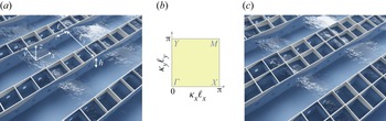
In the present study, we analyse the dispersion of a periodic medium with subwavelength resonators inspired by the recent works of Euvé et al. (Reference Euvé, Pham, Petitjeans, Pagneux and Maurel2021a,Reference Euvé, Piesniewska, Maurel, Pham, Petitjeans and Pagneuxb). The medium is composed of alternating open canals and resonant canals formed by one or two resonators; see figure 1. The resonators are cavities whose vertical walls extend through the entire depth of the fluid, with completely submerged holes drilled on two opposite walls. We will consider the case where the resonant canal contains a single resonator, called a single-resonant canal (figure 1a) and the case where the resonant canal contains two connected resonators, called a doubly-resonant canal (figure 1c). Our analysis is based on the Bloch–Floquet formalism combined with asymptotics using an underlying scale separation; this is developed in § 2 (the Brillouin zone is shown in figure 1(b) with  ${\boldsymbol \kappa }=(\kappa _x,\kappa _y)$ the Bloch–Floquet wavenumber). The derivation of the dispersion relation for a single-resonant canal is performed in § 3, and the exercise is repeated more briefly for a doubly-resonant canal in § 4. We show that the dispersion relation can be put in the same form in both cases, namely
 \begin{equation} \frac{\kappa_x^2}{\kappa_0^2}+\left(\chi_s-\chi_a\right)\sin^2 \frac{\kappa_y\ell_y}{2}=\chi_s, \end{equation}
where  $\chi _s$ and
 $\chi _a$ are explicit frequency-dependent functions (which depend on the number of resonators in the resonant canal) that encapsulate the subwavelength resonances of the symmetric and antisymmetric modes. In particular, we show that the dispersion is governed by a geometrical parameter that is the ratio of the cross-sections of the resonator and the open canal in the unit cell, analogous to the hopping parameter in SSH systems (see e.g. Coutant et al. Reference Coutant, Sivadon, Zheng, Achilleos, Richoux, Theocharis and Pagneux2021). Finally, in § 5, the complete band diagrams of both structures are analysed, revealing transitions from elliptical to hyperbolic dispersions, similar to the topological transitions in the isofrequency surfaces of optical metamaterials alternating subwavelength layers of metal and dielectric (Dyachenko et al. Reference Dyachenko, Molesky, Petrov, Störmer, Krekeler, Lang, Ritter, Jacob and Eich2016); in both cases, the anisotropic medium is characterized by an effective water depth tensor. In the hyperbolic regime, one of the water depths is negative and an application to negative refraction is proposed. Throughout the course of our study, the validation of the theoretical results is proposed through the comparison with numerical calculations of the full three-dimensional problem.
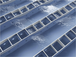
Conceptual view of arrays alternating open canals and resonant canals. (a) Single-resonant canals contain one resonator along  $y$. (b) The irreducible Brillouin zone with
 ${\boldsymbol \kappa }=(\kappa _x,\kappa _y)$ the Bloch–Floquet wavenumber. (c) Doubly-resonant canals contain two resonators along
 $y$.

2. Preliminaries
We consider an inviscid, incompressible fluid and an irrotational motion. Therefore, the velocity  ${\boldsymbol U}({\boldsymbol r})$ and the velocity potential
 $\varPhi ({\boldsymbol r})$ (where
 ${\boldsymbol r}=(x,y,z)$) are solutions of
 \begin{equation} {{\rm div}}\,{\boldsymbol U}=0,\quad {\boldsymbol U}={\boldsymbol{\nabla}} \varPhi. \end{equation}
We consider the harmonic regime with time dependence  $\exp ({-{\rm i}\omega t})$ (where
 $\omega$ is frequency, and
 $t$ is time). The boundary conditions read
 \begin{equation} U_z(x,y,0)=\frac{\omega^2}{g}\,\varPhi(x,y,0),\quad {\boldsymbol U}\boldsymbol{\cdot} {\boldsymbol n}=0\ \text{on the rigid walls}, \end{equation}
with the origin  $O$ at the mean free surface and
 $z$ directed vertically upwards, and where
 $U_z$ is the vertical component of the velocity,
 ${\boldsymbol n}$ is the normal to the rigid part boundaries, and
 $g$ is the gravitational constant.
2.1. Separation of the scales
We consider resonant cavities whose vertical walls extend through the entire depth  $h$ of the fluid, with completely submerged holes drilled on two opposite walls. The dynamics of a resonator are captured through the separation of three scales similar to that used in Euvé et al. (Reference Euvé, Pham, Petitjeans, Pagneux and Maurel2021a). The smallest, microscopic scale is associated with the dimensions of the hole: its width
 $e$, which is also the width of the vertical walls, and
 $\sqrt {s}$, with
 $s$ its cross-section. The intermediate, mesoscopic scale is associated with the dimensions of the three-dimensional unit cell,
 $\ell _x$,
 $\ell _y$ and
 $h$. Finally, the largest, macroscopic scale refers to the wavelength
 $1/k=\sqrt {gh}/\omega$ of the waves that would propagate in the absence of resonators (i.e. at the free surface of the water column of depth
 $h$ in the shallow-water regime). We emphasize that this does not imply that the effective wavenumber
 ${\kappa }$ supported by the metamaterial behaves in the same way, and therefore in (1.1) we do not have necessarily
 $\sin (\kappa _y\ell _y/2)\simeq (\kappa _y\ell _y)/2$. We also define
 \begin{equation} S_c=\ell_c^2,\quad S=\ell\ell_x \end{equation}
as the cross-sections of the resonant cavity and the open canal, with  $\ell _c=\ell _x-e$ and
(i)
 $\ell =\ell _y-\ell _c-2e$ for the single-resonant canal,
(ii)
$\ell =\ell _y-2\ell _c-3e$ for the doubly-resonant canal.


We thus have
 \begin{equation} \sqrt{s}, e \ll \ell_c, \ell, \ell_x, \ell_y, h \ll 1/k, \end{equation}
and, as said before, the wavelength  $1/k$ at the largest scale indicates a low-frequency regime, not a large effective wavelength
 $1/\kappa$.
With this separation of scales, the analysis of the problem is similar to that of Marigo, Maurel & Pham (Reference Marigo, Maurel and Pham2023). It combines an asymptotic homogenization along  $x$ and a Bloch–Floquet analysis along
 $y$. The homogenization allows us to establish the effective propagation equation in the
 $x$ direction, which provides in part the characteristics of the effective medium. The Bloch–Floquet condition allows us to take into account the values of
 $\kappa _y \in (0,{\rm \pi} /\ell _y)$, which is necessary to obtain the dispersion relations announced in (1.1). In §§ 2.2 and 3.1, we present informally the main steps of the analysis, the more formal derivation of which is given in Appendix A.
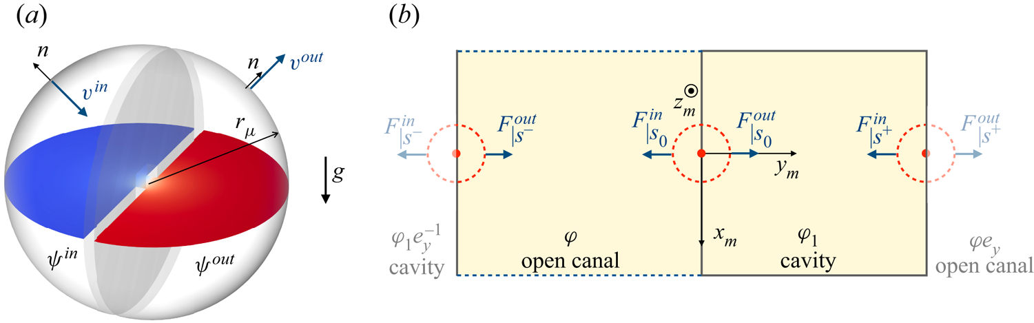
2.2. Fluxes and potentials at the microscopic scale
At the microscopic scale, i.e. near the opening in the wall, the problem is still that of a potential flow in three dimensions, but the geometry is simplified greatly since the wall has an infinite extension. We consider the problem in a dimensionless form for a hole of unit section in a wall of thickness  $e/\sqrt {s}$ separating two unbounded regions
 $\varOmega ^{in}$ and
 $\varOmega ^{out}$ (figure 2a). Accordingly, we define
 \begin{equation} {\boldsymbol r}_{\mu}=\frac{{\boldsymbol r}}{\sqrt{s}},\quad \psi\left(\frac{{\boldsymbol r}}{\sqrt{s}}\right)=\varPhi({\boldsymbol r}),\quad {\boldsymbol v}\left(\frac{{\boldsymbol r}}{\sqrt{s}}\right)=\sqrt{s}\,{\boldsymbol U}({\boldsymbol r}), \end{equation}
and the potential  $\psi$ and velocity
 ${\boldsymbol v}$ satisfy
 \begin{equation}
{\boldsymbol
v}={\boldsymbol{\nabla}}_{\mu} \psi,
\quad {\rm
div}_{\mu}\,{\boldsymbol v}=0,\quad {\boldsymbol
v}\underset{r_{\mu}\to
+\infty}{\sim}\left\{\begin{array}{@{}ll} \displaystyle
-\dfrac{A}{2{\rm \pi} r_{\mu}}\,{\boldsymbol n}, & \text{in }
\varOmega^{in},\\ \displaystyle \dfrac{A}{2{\rm \pi}
r_{\mu}}\,{\boldsymbol n}, & \text{in } \varOmega^{out},
\end{array}\right. \end{equation}
with  ${\boldsymbol v}\boldsymbol {\cdot } {\boldsymbol n}=0$ on the rigid parts, and where
 $A$ is the flux. The solution is written in the form
 $\psi ({\boldsymbol r}_{\mu })=A\,f({\boldsymbol r}_{\mu })+B$, with
 $A$ and
 $B$ two constants and
 \begin{equation} f({\boldsymbol r}_{\mu})\underset{r_{\mu}\to +\infty}{\sim} \left\{\begin{array}{@{}ll} \displaystyle \dfrac{1}{2{\rm \pi} r_{\mu}}-\dfrac{b}{2}, & \text{in } \varOmega^{in}, \\ \displaystyle -\dfrac{1}{2{\rm \pi} r_{\mu}}+\dfrac{b}{2}, &\text{in } \varOmega^{out}, \end{array}\right. \end{equation}
where  $b$ is a blockage coefficient. We also obtain the form of the constant potentials far from the hole,
 $\psi ^{in}=-Ab/2+B$ in
 $\varOmega ^{in}$, and
 $\psi ^{out}=Ab/2+B$ in
 $\varOmega ^{out}$, and thus
 \begin{equation} A=\frac{1}{b}\,(\psi^{out}-\psi^{in}). \end{equation}
(a) Potential flow problem through a pierced wall between two semi-infinite domains (microscopic scale). The horizontal section shows the potential  $\psi ({\boldsymbol r}_{\mu })$ calculated numerically for a hole with unit section (red and blue indicate the maximum and minimum values of
 $\psi$, respectively). (b) Unit cell at the mesoscopic scale for the single-resonant canals. The potentials are constant within each domain (open canal and resonant cavity), and the Bloch–Floquet condition applies between adjacent cells.

We now return to our dimensional problem at the mesoscopic scale (figure 2b). The fluxes  $F^{in}$ and
 $F^{out}$ are obtained from the previous analysis thanks to the relation
 $F^{out}=-F^{in}=\sqrt {s}\,A$, which gives
 \begin{equation} F^{out}={-}F^{in}=\alpha(\varphi^{out}-\varphi^{in}),\quad \alpha=\frac{\sqrt{s}}{b}. \end{equation}
where  $\varphi ^{in}$ (resp.
 $\varphi ^{out}$) refer to the value of the potential on the left (resp. on the right) of the drilled hole. For a given shape of the hole, the solution of the potential flow problem, posed on
 $\psi ({\boldsymbol r}_{\mu })$, can be computed numerically by fixing
 $A=1$, which gives the constant
 $b$ (see § B.1). The value of
 $b$ depends on
 $e/\sqrt {s}$ and the shape of the hole cross-section. In Appendix C, we report the variations of
 $b(e/\sqrt {s})$ computed for a square-shaped hole.
3. The case of single-resonant canals
In this section, we derive the dispersion relation announced in (1.1) along with the closed form of the functions  $\chi _s$ and
 $\chi _a$ for the configuration of figure 1(a) alternating open canals and single-resonant canals. The dispersion along the main directions of the Brillouin zone is discussed in relation to the geometrical parameter
 $\gamma =S_c/S$, the increase of which produces the closure and re-opening of a band-gap along
 $\varGamma Y$.
3.1. Effective propagation
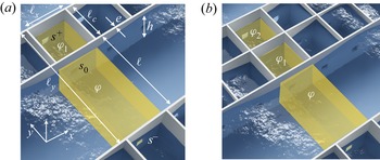
In the three-dimensional unit cell sketched in figure 3(a), we introduce the mesoscopic coordinate  ${\boldsymbol r}_{m}={\boldsymbol r}/h$, where
 $r_{m}=(x_{m},y_{m},z_{m}$). The result of the asymptotic analysis, whose details are given in Appendix A, is as follows. The resonant cavity is closed by walls except at the free surface, and we have
 \begin{equation} \text{in the cavity,}\quad \varPhi({\boldsymbol r})=\varphi_1(x),\quad {\boldsymbol U}({\boldsymbol r})= {\boldsymbol w}_1(x,{\boldsymbol r}_{m}), \end{equation}
satisfying
 \begin{equation} {{\rm div}}_{m}\,{\boldsymbol w}_1=0,\quad {\boldsymbol w}_1(x,x_{m},y_{m},0)\boldsymbol{\cdot} \boldsymbol{e}_z=\frac{\omega^2}{g}\,\varphi_1(x), \end{equation}
and  ${\boldsymbol w}_1\boldsymbol {\cdot } {\boldsymbol n}=0$ on the walls. Next, the region of the open canal is bounded by walls along
 $y$ only, and we have
 \begin{equation} \text{in the open canal,}\quad \varPhi({\boldsymbol r})=\varphi(x),\quad {\boldsymbol U}({\boldsymbol r})=\frac{\partial \varphi}{\partial x}(x)\,\boldsymbol{e}_x+ {\boldsymbol w}(x,{\boldsymbol r}_{m}), \end{equation}
satisfying
 \begin{equation} \frac{\partial^2 \varphi}{\partial x ^2}+{{\rm div}}_{m}\,{\boldsymbol w}=0,\quad {\boldsymbol w}(x,x_{m},y_{m},0)\boldsymbol{\cdot} \boldsymbol{e}_z=\frac{\omega^2}{g}\,\varphi(x), \end{equation}
 ${\boldsymbol w}\boldsymbol {\cdot } {\boldsymbol n}=0$ on the walls, and a periodic boundary condition between
 $x_{m}=\pm \ell _x/2$.
Unit cells (highlighted regions) used to derive the effective propagation (a) for the single-resonant canals and (b) for the doubly-resonant canals.

Note that at the mesoscopic scale, the holes are reduced to points, and at these points, the velocities  $({\boldsymbol w},{\boldsymbol w}_1)$ have a singularity in
 $|{\boldsymbol r}_{m}|^{-2}$ that guarantees finite fluxes. These finite fluxes are given by the analysis at the microscopic scale that provided (2.9). Hence with
 $F^{in/out}_{|s}(x)=\int _{s^{in/out}} {\boldsymbol w}(x,{\boldsymbol r}_{m})\boldsymbol {\cdot } \boldsymbol {e}_{{\boldsymbol r}_{m}} \,\text {d} s$ – the fluxes through the surfaces
 $s^{in/out}$ of the half-spheres centred at a singular point with vanishing radius – we obtain
 \begin{equation} F^{out}_{|s}(x)={-}F^{in}_{|s}(x)=\alpha (\varphi_{|s}^{out}(x)-\varphi_{|s}^{in}(x)). \end{equation}
We will now derive the equation governing the effective propagation along  $x$ and take into account the Bloch–Floquet condition along
 $y$, i.e. when passing from one cell to the others over large distances. To begin with, we integrate the incompressibility relation in (2.2a,b) within a resonant cavity, and we obtain
 \begin{equation} \frac{\omega^2S_c}{g}\,\varphi_1-F^{out}_{|{s_0}}-F^{in}_{|{s^+}}=0, \end{equation}
with  $F^{out}_{|{s_0}}$ and
 $F^{in}_{|{s^+}}$ defined in figure 2(a). Accordingly, we have
 $\varphi ^{in}_{|{s_0}}=\varphi$,
 $\varphi ^{out}_{|{s_0}}=\varphi ^{in}_{|{s^+}}=\varphi _1$ and, accounting for the Bloch–Floquet conditions along adjacent cells,
 $\varphi ^{out}_{|{s^+}}=\varphi e_y$ (where
 $e_y=\exp ({{\rm i}\kappa _y\ell _y})$), hence
 \begin{equation} \frac{\omega^2S_c}{g}\,\varphi_1-\alpha(\varphi_1-\varphi)+\alpha(\varphi e_y-\varphi_1)=0. \end{equation}
Next, we integrate the incompressibility relation in (3.4a,b) in the region of the open canal, resulting in
 \begin{equation} S h\,\frac{\partial^2 \varphi}{\partial x ^2}+\frac{\omega^2S}{g}\,\varphi-F^{out}_{|{s^{-}}}-F^{in}_{|{s_0}}=0, \end{equation}
with  $\varphi ^{in}_{|{s^{-}}}=\varphi _1e_y^{-1}$,
 $\varphi ^{out}_{|{s^{-}}}=\varphi ^{in}_{|{s_0}}=\varphi$ and
 $\varphi ^{out}_{|{s_0}}=\varphi _1$, and thus the second relation
 \begin{equation} S h\,\frac{\partial^2 \varphi}{\partial x ^2}+\frac{\omega^2S}{g}\,\varphi-\alpha(\varphi-\varphi_1e_y^{{-}1})+\alpha(\varphi_1-\varphi)=0. \end{equation}
By defining the quantities
 \begin{equation} \omega_0^2=\frac{\alpha g}{S_c},\quad \kappa_0^2=\frac{\omega_0^2}{gh},\quad \gamma=\frac{S_c}{S}, \end{equation}
and the non-dimensional frequency  $\varOmega =\omega /\omega _0$, (3.7) and (3.9) take the form
 \begin{equation} \left\{\begin{array}{@{}l} (\varOmega^2-2)\varphi_1+(1+e_y)\varphi=0,\\ \displaystyle \dfrac{1}{\kappa_0^2}\,\dfrac{\partial^2 \varphi}{\partial x ^2}+(\varOmega^2-2\gamma)\varphi +\gamma(1+e_y^{{-}1})\varphi_1=0. \end{array}\right. \end{equation}
In the limit  $\gamma =0$, we recover the one-dimensional propagation equation for a stratified medium, namely
 $\partial _{xx}\varphi +(\omega ^2/gh) \varphi =0$, as it should be (Porter Reference Porter2021); see also Appendix D.
3.2. Dispersion and symmetries of the modes
The dispersion and associated modes are obtained by looking for  $\varphi (x)=\varphi \exp ({{\rm i}\kappa _x x})$ and
 $\varphi _1(x)=\varphi _1 \exp ({{\rm i}\kappa _x x})$ in (3.11), which takes the form
 \begin{equation} \left\{\begin{array}{@{}l} (\varOmega^2-2) \varphi_1+(1+e_y)\varphi=0,\\ \gamma(1+e_y^{{-}1})\varphi_1 +\left(\varOmega^2-2\gamma-(\kappa_x/\kappa_0)^2\right)\varphi=0. \end{array}\right. \end{equation}
The solvability condition of (3.12) provides the dispersion relation announced in (1.1) with
 \begin{equation} \chi_s(\varOmega)=\varOmega^2-2\gamma\,\frac{\varOmega^2}{\varOmega^2-2},\quad \chi_a(\varOmega)=\varOmega^2-2\gamma. \end{equation}
As a result, we obtain the following results along the principal directions of the Brillouin zone:
 \begin{equation} \begin{array}{@{}ll} \text{along $YM$,}\quad \left\{\begin{array}{@{}lll} \chi_s=\infty\ (\varOmega=\sqrt{2}), & \varphi=0, & \text{S mode,}\\ \kappa_x=\kappa_0\sqrt{\chi_a}, & \varphi_1=0, & \text{A mode,} \end{array}\right. \end{array} \end{equation}
 \begin{equation} \text{along}\ X\varGamma,\quad \kappa_x=\kappa_0\sqrt{\chi_s},\quad \frac{\varphi_1}{\varphi} ={-}\frac{2}{\varOmega^2-2},\quad\text{S mode}, \end{equation}
 \begin{equation} \left.\begin{array}{ll@{}} \text{along}\ \varGamma Y, & \dfrac{\varphi_1}{\varphi}={-}\dfrac{1+e_y}{\varOmega^2-2}, \\ & \text{with}\ \gamma(e_y+e_y^{{-}1})=\varOmega^4-2(\gamma+1)\varOmega^2+2\gamma \end{array}\right\} \end{equation}
(where the above dispersion is equivalent to (1.1) along with (3.13a,b) for  $\kappa _x=0$). Note that we call S mode (resp. A mode) a mode that is symmetric (resp. antisymmetric) with respect to the axis
 $(C,\boldsymbol {e}_x)$, with
 $C$ the centre of a resonant cavity (that is, within a shifted unit cell with
 $y_{m}\in (-\ell _y/2,\ell _y/2)$).
The system (3.12) is degenerate at  $Y$ (
 $\kappa _x=0$,
 $e_y=-1$) for
 $\gamma =1$ since the discriminant of the system vanishes. From (3.14), this corresponds to the point where the branch of the S mode at
 $\varOmega =\sqrt {2}$ (the pole of
 $\chi _s$) meets the branch
 $\kappa _x=\kappa _0\sqrt {\chi _a}$ of the A mode at
 $\kappa _x=0$ (with
 $\chi _a=\varOmega ^2-2$ for
 $\gamma =1$). We will see that this corresponds to the appearance of a Dirac point at
 $Y$.
To inspect the validity of the obtained dispersion, we consider the following configurations. The resonators have a square cross-section  $S_c=\ell _c^2$ with
 $\ell _c=5$ cm and wall thickness
 $e=0.2$ cm. Then we fix the length of the open canal
 $\ell$ to obtain
 $\gamma =0.5$, 1 or 2 (hence
 $\ell \simeq 9.6$, 4.8 or 2.4 cm). The (square) section of the submerged opening is
 $s=0.5\times 0.5$ cm
 $^2$, and the water depth is
 $h=5$ cm. The analysis of potential flow through the opening provides the blockage coefficient
 $b=1.31$ (see Appendix C) and accordingly,
 $\omega _0=3.87$ rad s
 $^{-1}$ and
 $\kappa _0=5.52$ m
 $^{-1}$.
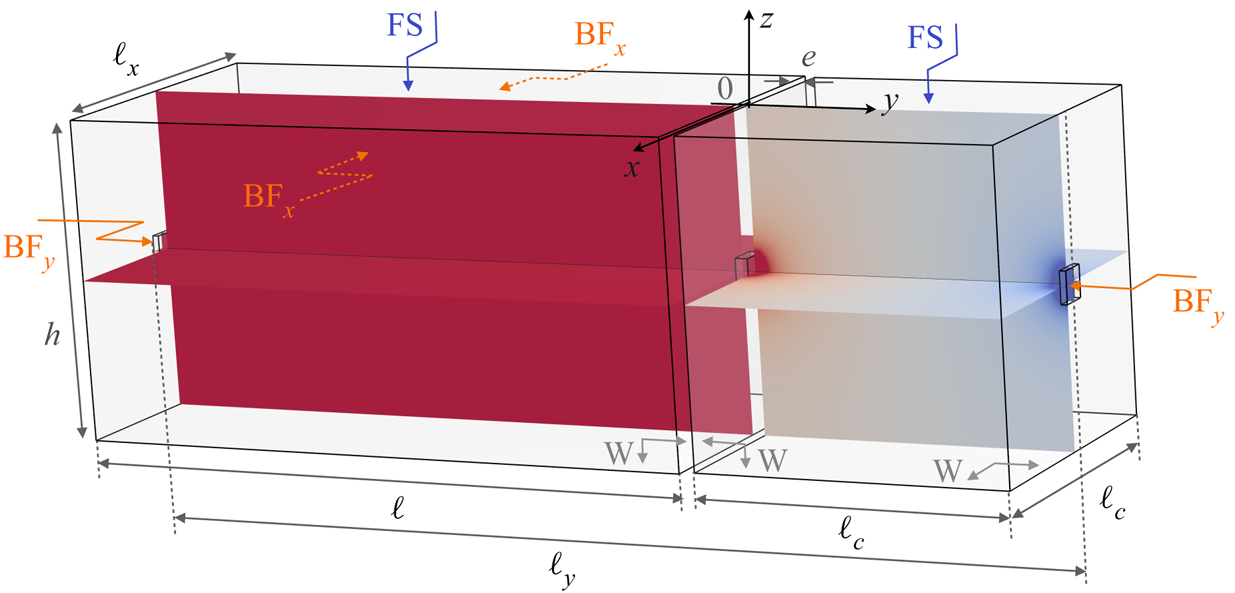
The dispersion in the actual three-dimensional unit cell was calculated numerically. The unit cell is shown in figure 4 for  $\ell =10$ cm. This has been done by using Bloch–Floquet conditions along
 $y$ (BF
 $_y$ on faces opposite of the holes at
 $y=0$ and
 $y=-\ell _y$) and along
 $x$ (on faces opposite
 $x=\pm \ell _x/2$ and
 $y\in (-(\ell _c+e), -\ell _y)$), a free water surface condition FS at
 $z=0$ (except on regions of the resonator walls piercing the free surface), and a rigid wall condition W on the submerged resonator walls and on the sea bottom (see details of the numerics in § B.2). In the following, we restrict our representation to
 $\varGamma Y'$ with
 $Y'$(
 $\kappa _y=0,\ \kappa _x\ell _y={\rm \pi} )$ and
 $XM'$ with
 $M'$(
 $\kappa _y\ell _y={\rm \pi},\ \kappa _x\ell _y={\rm \pi} )$ since the branches along these directions reach their asymptotes well before
 $\kappa _x\ell _x={\rm \pi}$.
Geometry of the three-dimensional unit cell used to compute numerically the dispersion and the Bloch–Floquet modes, and boundary conditions used in the calculations (see main text), with  $\ell _y=\ell _c+\ell +2e$ and
 $\ell _x=\ell _c+e$.

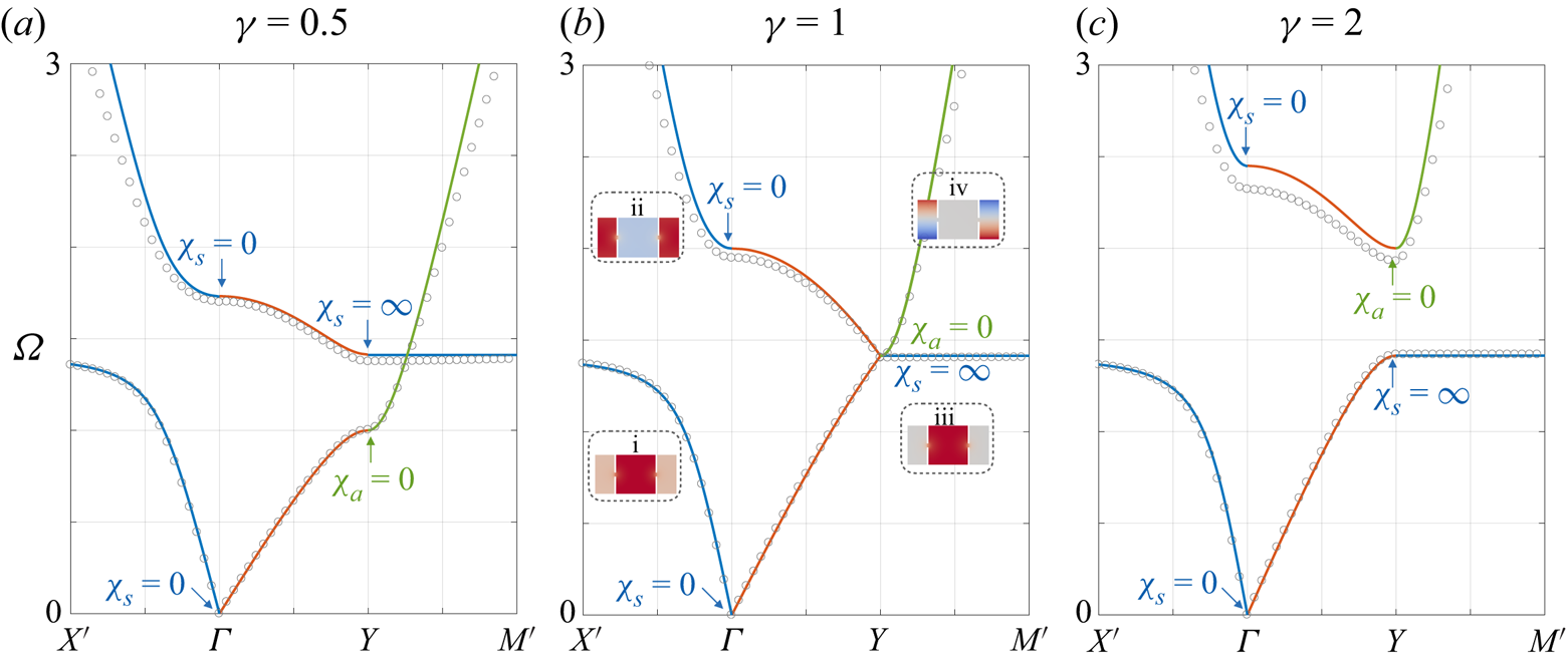
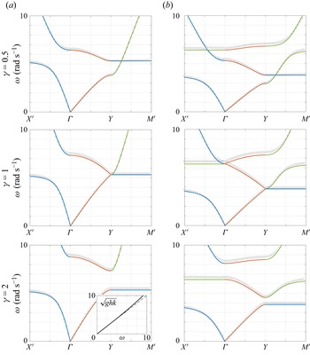
The numerical results are presented in figure 5 (grey symbols) together with our theoretical prediction, (1.1) with (3.13a,b) (solid lines). We observe very good agreement, with, however, a slight loss of accuracy when  $\varOmega$ increases since the assumption of constant potential inside the resonant cavity becomes questionable and at the same time we leave the shallow-water regime. Note that an adaptation to greater water depth is possible; this is discussed in Appendix E.
Dispersion along the principal directions of the Brillouin zone for the single-resonant canal. The grey symbols are from the direct numerics, and the solid lines are from (1.1) with (3.13a,b). Along  $X'\varGamma$, the two branches are associated with S modes; along
 $YM$, the blue branch is associated with S modes (
 $\varphi =0$), the green branch with A modes (
 $\varphi _1=0$). In (b), the insets show the patterns in the unit cell centred on the resonator. Because of the degeneracy at
 $Y$ for
 $\gamma =1$, the gap along
 $\varGamma Y$ at
 $\gamma =0.5$ closes at
 $\gamma =1$, and re-opens at
 $\gamma =2$.

Let us now comment on the observed dispersion in the light of the general properties given in (3.14)–(3.16). The two eigenfrequencies at  $\varGamma$ are
 $\varOmega =0,\sqrt {2(\gamma +1)}$ (
 $\chi _s=0$), and the S mode along
 $X'\varGamma$ follows the two parts of the branch
 $\kappa _x=\kappa _0\sqrt {\chi _s}$ corresponding to
 $\chi _s>0$. Consequently, a band-gap for
 $\varOmega \in (\sqrt {2},\sqrt {2(\gamma +1)})$ is observed for any
 $\gamma$. The two eigenfrequencies at
 $Y$ are
 $\varOmega =\sqrt {2},\sqrt {2\gamma }$ (
 $\chi _s=\infty$ for the S mode, and
 $\chi _a=0$ for the A mode). Along
 $YM$, the branch of the S mode stays glued to its asymptote at
 $\varOmega =\sqrt {2}$, and the A mode follows the part of the branch
 $\kappa _x=\kappa _0\sqrt {\chi _a}$ corresponding to
 $\chi _a>0$ (
 $\varOmega >\sqrt {2\gamma }$). (For
 $\gamma <1$, our model predicts that the two branches along
 $YM'$ intersect at
 $\varOmega =\sqrt {2}$; in the direct numerics, we observe an avoiding crossing.) As expected, the relative positions of the two branches vary depending on whether
 $\gamma <1$ or
 $\gamma >1$, and they cross for
 $\gamma =1$. As a result, the band-gap opens along
 $\varGamma Y$ for
 $\gamma <1$, closes at
 $Y$ for
 $\gamma =1$ with the appearance of a Dirac point, and re-opens for
 $\gamma >1$. This behaviour is characteristic of topological systems studied recently in the context of water waves (Yang et al. Reference Yang, Gao and Zhang2016; Anglart Reference Anglart2021); see also Coutant et al. (Reference Coutant, Sivadon, Zheng, Achilleos, Richoux, Theocharis and Pagneux2021) in one-dimensional and Zheng et al. (Reference Zheng, Achilleos, Richoux, Theocharis and Pagneux2019) in two-dimensional acoustic systems.
We conclude this discussion by commenting on the shapes of modes reported in the insets in figure 5(b) for  $\gamma =1$. Along
 $X'\varGamma$, the modes are symmetric; in agreement with (3.15), we observe that
 $\varphi _1/\varphi$ is positive on the first branch (inset i), and it is negative on the second branch (inset ii). The first branch then reaches its asymptote at
 $\varOmega =\sqrt {2}$, giving rise to a symmetric mode extended along
 $YM$, with
 $\varphi =0$ in agreement with (3.14) (inset iii). The second branch along
 $YM$ is associated with antisymmetric modes, which is made possible for the single-resonant canal since
 $\varphi _1=0$, in agreement with (3.14) (inset iv). The degeneracy at
 $Y$ is again visible as the shapes of the S and A modes become incompatible at
 $Y$.
4. The doubly-resonant canal
We now turn to the configuration in figure 1(c). The unit cell is composed of two identical resonators and a region of the open canal. The second resonator introduces an additional degree of freedom while preserving the form of the dispersion (only  $\chi _s$ and
 $\chi _a$ will be different), which facilitates the interpretation of the observed phenomena.
4.1. Analysis of the effective propagation
We proceed as in the previous section, starting with the integration of the incompressibility relation in (2.2a,b) in each resonator, which applies for  $\varPhi ({\boldsymbol r})=\varphi _1(x)$ and
 $\varPhi ({\boldsymbol r})=\varphi _2(x)$; see figure 3(b). We obtain
 \begin{equation} \left\{\begin{array}{@{}l} (\varOmega^2-2)\varphi_1+\varphi_2={-}\varphi,\\ \varphi_1 +(\varOmega^2-2)\varphi_2={-}e_y\varphi, \end{array}\right. \end{equation}
where  $e_y=\exp ({{\rm i}\kappa _y \ell _y})$, and with now
 $\ell _y=2\ell _c+\ell +3e$. Next, we use (3.4a,b) that we integrate over the region of the open canal within the unit cell, and we obtain
 \begin{equation} S h\,\frac{\partial^2 \varphi}{\partial x ^2}+\frac{\omega^2S}{g}\,\varphi+\alpha(\varphi_1+\varphi_2 e_y^{{-}1}-2\varphi)=0. \end{equation}
4.2. Dispersion and symmetries of the modes
With two resonators, the analysis of the Bloch–Floquet mode symmetry is simplified greatly by introducing the symmetric and antisymmetric parts of the modes in the resonators  $\varphi _a=(\varphi _1+\varphi _2)/2$ and
 $\varphi _s=(\varphi _1-\varphi _2)/2$. Next, as before, we look for
 $\varphi (x)=\varphi \exp ({{\rm i}\kappa _x x})$ and
 $\varphi _{s,a}(x)=\varphi _{s,a} \exp ({{\rm i}\kappa _x x})$. By doing so, we obtain from (4.1) and (4.2) the equivalent system
 \begin{equation} \left\{\begin{array}{@{}l} 2\left(\varOmega^2-1\right)\varphi_s+(1+e_y)\varphi=0,\\ 2\left(\varOmega^2-3\right)\varphi_a+(1-e_y)\varphi=0,\\ \gamma(1+e_y^{{-}1})\varphi_s+\gamma(1-e_y^{{-}1})\varphi_a +\left(\varOmega^2-2\gamma-(\kappa_x/\kappa_0)^2 \right)\varphi=0, \end{array}\right. \end{equation}
whose solvability condition provides the dispersion relation. We recover the form announced in (1.1), with  $\chi _s$ and
 $\chi _a$ given by
 \begin{equation} \chi_s(\varOmega)=\varOmega^2-2\gamma\,\frac{\varOmega^2}{\varOmega^2-1},\quad \chi_a(\varOmega)=\varOmega^2-2\gamma\,\frac{\varOmega^2-2}{\varOmega^2-3} \end{equation}
(instead of (3.13a,b)), with  $(\gamma,\kappa _0,\omega _0)$ given in (3.10a–c) and still
 $\varOmega =\omega /\omega _0$. Along the principal directions of the Brillouin zone, we obtain
 \begin{gather} \begin{array}{@{}ll} \text{along}\ YM:\quad \left\{\begin{array}{@{}lll} \chi_s=\infty (\varOmega=1), & \varphi=\varphi_a=0,\quad & \text{S mode,}\\ \kappa_x=\kappa_0\sqrt{\chi_a}, & \varphi_s=0,\quad \dfrac{\varphi_a}{\varphi}={-}\dfrac{1}{\varOmega^2-3}, & \text{A mode}, \end{array}\right. \end{array} \end{gather}
 \begin{gather} \begin{array}{@{}ll} \text{along}\ X\varGamma: \quad \left\{\begin{array}{@{}lll} \chi_a=\infty\ (\varOmega=\sqrt{3}), & \varphi=\varphi_s=0, & \text{A mode},\\ \kappa_x=\kappa_0\sqrt{\chi_s}, & \varphi_a=0,\quad \dfrac{\varphi_s}{\varphi}={-}\dfrac{1}{\varOmega^2-1}, & \text{S mode}, \end{array}\right. \end{array} \end{gather}
 \begin{gather} \left.\begin{array}{@{}ll} \text{along}\ \varGamma Y: & \dfrac{\varphi_s}{\varphi}={-}\dfrac{e_y+1}{2(\varOmega^2-1)},\quad \dfrac{\varphi_a}{\varphi}=\dfrac{e_y-1}{2(\varOmega^2-3)}, \\ & \text{with}\quad \gamma(e_y+e_y^{{-}1})+\varOmega^2(\varOmega^4-4\varOmega^2+3)-2\gamma(\varOmega^4-3\varOmega^2+1)=0, \end{array}\right\} \end{gather}
where the above dispersion relation is equivalent to (1.1) with (4.4a,b), for  $\kappa _x=0$. (Note that the symmetries of the modes correspond to symmetries with respect to
 $Cx_{m}$, with
 $C$ the centre between the cavities and
 $y_{m}\in (-\ell _y/2,\ell _y/2)$.) The situation is now the same at
 $\varGamma$ and
 $Y$. At
 $\varGamma$, the eigenfrequencies correspond to the two zeros of
 $\chi _s$ and the pole of
 $\chi _a$, and at
 $Y$, the eigenfrequencies correspond to the two zeros of
 $\chi _a$ and the pole of
 $\chi _s$.
For  $\gamma =1$, the system (4.3) is degenerate at
 $Y$ when
 $\varOmega =1$, and it is degenerate at
 $\varGamma$ when
 $\varOmega =\sqrt {3}$ (the discriminant of the system (4.3) vanishes). In the former case at
 $Y$, the scenario is the same as for the single-resonant canal; from (4.5), the branch of the S mode at
 $\varOmega =1$ (the pole of
 $\chi _s$) meets the branch
 $\kappa _x=\kappa _0\sqrt {\chi _a}$ of the A mode at
 $\kappa _x=0$ (with
 $\chi _a=(\varOmega ^2-1)(\varOmega ^2-4)/(\varOmega ^2-3)$ for
 $\gamma =1$). The situation is the same at
 $\varGamma$ for
 $\varOmega =\sqrt {3}$; from (4.6), the branch of the A mode at
 $\varOmega =\sqrt {3}$ (the pole of
 $\chi _a$) meets the branch
 $\kappa _x=\kappa _0\sqrt {\chi _s}$ of the S mode at
 $\kappa _x=0$ (with
 $\chi _s=\varOmega ^2(\varOmega ^2-3)/(\varOmega ^2-1)$ for
 $\gamma =1$). This will lead to the appearance of two Dirac points at
 $Y$ and at
 $\varGamma$.
We consider the same resonant cavities and open canal, hence again  $\gamma =0.5$, 1 and 2. The holes are the same, so
 $b=1.31$, and
 $\omega _0=3.87$ rad s
 $^{-1}$,
 $\kappa _0=5.52$ m
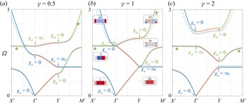
 $^{-1}$. Our representation in figure 6 is identical to that in figure 5 (with
 $\ell _y=2\ell _c+\ell +3e$). The dispersion in the three-dimensional unit cell has been calculated numerically (grey symbols) and is compared with the model (1.1) and (4.4a,b) (solid lines). We observe the same very good overall agreement as in figure 5. Among the three branches, two of them were already visible for the single-resonant canals, but with the appearance of a new antisymmetric branch (indicated by a star), the branches associated with the S and A modes now behave in the same way. Along
 $X\varGamma$, the two symmetric branches follow the dispersion
 $\kappa _x=\kappa _0\sqrt {\chi _s}$ with a band-gap when
 $\varOmega \in (1,\sqrt {1+2\gamma })$; the antisymmetric branch is glued to its asymptote at
 $\varOmega =\sqrt {3}$ (
 $\chi _a=\infty$). Consequently, a Dirac cone appears at
 $\varGamma$ where the two branches meet, for
 $\gamma =1$,
 $\varOmega =\sqrt {3}$. Along
 $YM'$, the two antisymmetric branches follow the dispersion
 $\kappa _x=\kappa _0\sqrt {\chi _a}$ with two band-gaps when
 $\varOmega \in (0,\varOmega ^-)$ and
 $\varOmega \in (\sqrt {3},\varOmega ^+)$ (
 $\chi _a<0$, with
 $\varOmega ^\pm$ the two zeros of
 $\chi _a$). (The two zeros
 $\varOmega ^\pm$ of
 $\chi _a$ are the roots of
 $\varOmega ^4-(3+2\gamma )\varOmega ^2+4\gamma =0$, and whatever the value of
 $\gamma$,
 $\varOmega ^-\in (0,\sqrt {2})$ and
 $\varOmega ^+\in (\sqrt {3},+\infty )$.) The symmetric branch is glued to its asymptote at
 $\varOmega =1$ (
 $\chi _s=\infty$). With
 $\varOmega ^-=1$ when
 $\gamma =1$, the two branches meet when
 $\varOmega =1$, which gives a Dirac cone at
 $Y$.
Dispersion along the principal directions of the Brillouin zone for the doubly-resonant canal. Same representation as in figure 5. A new branch appears (green stars) associated with the pole of  $\chi _a$ and one of its two zeros, associated with A modes along
 $X'\varGamma$ and
 $YM'$. Because of the degeneracies at
 $\varGamma$ and
 $Y$, the gaps at
 $\gamma =0.5$ close at
 $\gamma =1$ and re-open at
 $\gamma =2$.

The shapes of the modes i–iv (shown in the insets of figure 6b) on the branches that existed for a single-resonant canal are identical to those reported in figure 5, with  $\varphi _a=0$ for i, ii, iv, and
 $\varphi _a=\varphi _s=0$ for iii. The new antisymmetric modes, v with
 $\varphi _s=\varphi =0$ and vi with
 $\varphi _s=0$, are made possible by the additional degree of freedom that we introduced with the second resonator.
5. Elliptic and hyperbolic dispersion, application to negative refraction
In this section, we take the usual representation of effective media in electromagnetism whose simple counterpart for water waves can be deduced from (1.1) when  $\kappa _y\ell _y\ll 1$. In this limit, the dispersion relation (1.1) provides, in dimensional form,
 \begin{equation} h_x\kappa_x^2+h_y\kappa_y^2=\frac{\omega^2}{g_e}, \end{equation}
with
 \begin{equation} h_x=h,\quad h_y=\frac{(\ell_y\omega_0)^2}{4g}\,(\chi_s-\chi_a),\quad g_e=\frac{\varOmega^2}{\chi_s}\,g. \end{equation}
The water-depth tensor (with diagonal elements  $(h_x,h_y)$) is equivalent to the permittivity tensor, and the effective gravity
 $g_e$ is equivalent to the effective permeability. With
 $h_x=h>0$, the dispersion is elliptical in nature when
 $h_y>0$ and
 $g_e>0$, and hyperbolic when
 $h_y<0$ (the negative index thought by Veselago (Reference Veselago1968), with
 $h_x$,
 $h_y$ and
 $g_e$ negative, is not possible). In the limit
 $\kappa _y\ell _y\ll 1$, we also obtain that the group velocity
 ${\boldsymbol v}_g={\boldsymbol {\nabla }}_{\boldsymbol \kappa }\omega$ is
 \begin{equation} {\boldsymbol v}_g\propto h_x\kappa_x\boldsymbol{e}_x+h_y\kappa_y\boldsymbol{e}_y, \end{equation}
and  ${\boldsymbol v}_g$ is perpendicular to the isofrequency contour (the curve
 $(\kappa _x,\kappa _y)$ in (5.1) for constant
 $\omega$ value). It is sometimes objected that the directions of the group velocity and the Poynting vector may differ. However, the unambiguous derivation of the expression for the Poynting vector in the equation of energy conservation is made difficult by the fact that (1.1), or (5.1), does not provide an effective model. It is shown in Appendix F that by using a continuity argument with the case of thick plates piercing the free surface, the Poynting vector can be written as
 \begin{equation} {\boldsymbol {\rm \pi}}=2\omega\xi\,|\varphi|^2(h_x\kappa_x\boldsymbol{e}_x+h_y\kappa_y \boldsymbol{e}_y), \end{equation}
where  $\xi =\ell /\ell _y$ is the filling fraction of open canal in the unit cell. Note that when the condition
 $\kappa _y\ell _y\ll 1$ is not satisfied, (5.1) is still valid using
 $h_y\to h_y\,{\rm sinc}^2(\kappa _y\ell _y/2)$, and (5.3) is still valid using
 $h_y\to h_y\,{\rm sinc}(\kappa _y\ell _y)$ (with still
 ${\boldsymbol v}_g$ perpendicular to the isofrequency contour). (We use the function
 ${\rm sinc}(a)=\sin a/a$.)
5.1. Band structure and analysis of the isofrequency contours
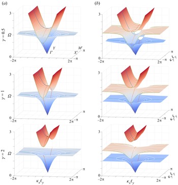
We are now interested in the complete band structure in the  $(\kappa _x,\kappa _y,\varOmega )$ space and in the analysis of the isofrequency contours. We plot in figure 7 the complete band structure obtained from (1.1), using
 $(\chi _s,\chi _a)$ in (3.13a,b) for the single-resonant canals and in (4.4a,b) for the doubly-resonant canals. The colours on the dispersion surfaces correspond to constant values of
 $\varOmega \in (0,3)$. We also plot isofrequency contours (white lines) and the dispersion along the principal directions of the Brillouin zone (coloured lines as in figures 5 and 6). To interpret the observed isofrequency contours, we start with (5.1), which tells us that the isofrequency contours are elliptical if
 $(\chi _s-\chi _a)>0$ (
 $h_y>0$) and
 $\chi _s>0$ (
 $g_e>0$), and hyperbolic if
 $(\chi _s-\chi _a)<0$ (
 $h_y<0$, whatever the sign of
 $g_e$). Therefore, in this
 $\kappa _y\ell _y\ll 1$ approximation, we expect that for a single-resonant canal, with
 $(\chi _s-\chi _a)=-4\gamma /(\varOmega ^2-2)$, the dispersion is of hyperbolic shape for
 $\varOmega >\sqrt {2}$, and for a doubly-resonant canal, with
 $(\chi _s-\chi _a)=4\gamma /((\varOmega ^2-1)(\varOmega ^2-3))$, it is of hyperbolic shape for
 $\varOmega \in (1,\sqrt {3})$, whatever the value of
 $\gamma$. This is roughly consistent with what is observed in figure 7, but must be corrected as
 $\kappa _y\ell _y$ increases. Indeed, for elliptical and hyperbolic dispersions predicted by (5.1), propagation along
 $\varGamma Y$ is always possible (there is a solution at
 $\kappa _x=0$,
 $\kappa _y\neq 0$). In fact, the dispersion is elliptical or hyperbolic only in the pass-bands of
 $\varGamma Y$. Outside these regions, ellipses and hyperbolas are deformed by the opening of a gap at
 $\kappa _x=0$. This becomes critical for large enough
 $\varOmega$ above the last pass-band of
 $\varGamma Y$, where the dispersion becomes strongly anisotropic. According to (3.13a,b) or (4.4a,b), we then have
 $\chi _s=\chi _a\simeq \varOmega ^2$, thus the isofrequency contours reduce to the two lines
 $\kappa _x=\pm \omega /\sqrt {gh}$ as in Porter (Reference Porter2021); see also Appendix D.
Full band structures of (a) a single-resonant canal and (b) a doubly-resonant canal. The white lines show the isofrequency contours, and the coloured lines show the dispersion in the pass-bands along  $\varGamma Y$ (red lines),
 $YM'$ (blue lines) and
 $X\varGamma$ (green lines). As
 $\varOmega$ increases, the structures have a dispersion alternating elliptical and hyperbolic isofrequency contours, and end up above the last pass-bands of
 $\varGamma X$ with a dispersion similar to that of non-resonant closed cavities.

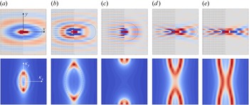
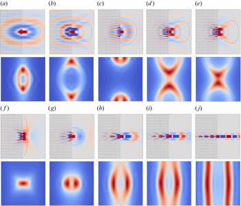
Directional emission of a point source through a single-resonant canal (top plots) and corresponding dispersion from the Fourier transform of the fields; the theoretical isofrequency contours, from (1.1) along with (3.13a,b), are shown with dashed black lines (bottom plots). Values of  $\varOmega$ used are (a) 0.62, (b) 1.12, (c) 1.61, (d) 1.92, and (e) 2.05.

To confirm and complete these theoretical predictions, we performed the following numerical experiments. We solved numerically the full three-dimensional problem with water depth  $h=5$ cm and, in the horizontal plane, a square domain of extension
 $30\ell _y\times 30\ell _y$. We impose a point excitation at frequency
 $\omega$ at the centre of the domain on the free surface corresponding to an open canal (details on the numerics are given in § B.3). The results are shown in figures 8 and 9 for the single- and doubly-resonant canals, respectively (the reported domain is
 $20\ell _y\times 20\ell _y$). In the figures, the upper plots show the velocity potential fields in the
 $(x,y)$ plane at the
 $z=0$ free surface. We plot for
 $x<0$ the raw numerical result (the position of the resonators is visible), and for
 $x>0$ we use a trick to reveal the effective propagation on
 $\varphi$ by expanding the field in the open canal to the entire unit cell. In these regions, the dashed black lines show the extremities of the Poynting vector calculated from (5.4). The lower plots show the Fourier transform of the field in the
 $(\kappa _x,\kappa _y)$ plane as well as the theoretical isofrequency contour at the same frequency (dashed black line).


The results confirm that the isofrequency contours undergo transitions between elliptical and hyperbolic shapes, and the agreement between direct numerical simulation and theory is very good. They also confirm the last transition to an ultra-directional emission along  $x$, similar to that of closed cavities, which results from the deformation of hyperbolas for single-resonant canals, and from the deformation of ellipses for doubly-resonant canals. We note that propagation in single-resonant canals is in general more anisotropic than in doubly-resonant canals. This is particularly visible in the hyperbolic regime, with a characteristic X-shaped emission, the X being less open for the upper plots in figure 8(d,e) than for those in figure 9(d,e).
5.2. Negative refraction produced by hyperbolic dispersion
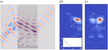
Negative refraction, as opposed to positive refraction, refers to a non-classical refraction whose most striking demonstration is made when a beam incident in a regular region is refracted on the same side of the normal to an interface with a metamaterial. To illustrate the ability of our hyperbolic media to produce negative refraction, we performed a numerical experiment in which such an incident beam passes through a slab  $x\in (0, L)$ surrounded by regular regions with constant water depth
 $h_0$. The slab is composed of simply resonant canals with the same characteristics as in § 3, and we used
 $L=18\ell _y$ and
 $h_0=h$. The incident beam is generated using sources pulsating at the frequency
 $\varOmega =2$, placed along a segment inclined at angle
 $\theta _i=45^\circ$ with respect to the vertical direction
 $y$. In figure 10(a), the incident beam interferes with the waves diffracted by the edges of the segment, but the beam emerging at
 $x=L$ is clearly visible with a well-defined angle
 $\theta _i$ and a small aperture. In the region
 $x>L$, the Fourier transform of the field thus produces a weak extension spot on the dispersion curve centred on
 ${\boldsymbol k}=k(\cos \theta _i,\sin \theta _i)$ with
 $k\ell _y= 1.23$; see figure 10(b).
(a) Negative refraction in a slab  $0< x< L$ made of resonant canals; the regions
 $x<0$ and
 $x>L$ corresponds to constant water-depth regions with water-depth
 $h_0=h$. The white arrows show the wavevectors inside and outside the slab, and the dashed red lines show the direction of the Poynting vectors. Wavevectors (white arrows) and Poynting vectors (red arrows) (b) outside and (c) inside the slab.

At the chosen frequency, the dispersion in the slab is of hyperbolic type. Since the vertical components of the wavevectors are conserved,  $\kappa _y\ell _y=k_y\ell _y=0.87$, we predict from (1.1) along with (3.13a,b) that
 $\kappa _x\ell _y=\pm 0.48$. To determine the sign of
 $\kappa _x$, we use the model again, and we are now interested in the Poynting vectors. Outside the slab,
 ${\boldsymbol {\rm \pi}}_0$ given by
 \begin{equation} {\boldsymbol {\rm \pi}}_0=2\omega\,|\varphi|^2h_0(k_x\boldsymbol{e}_x+k_y \boldsymbol{e}_y) \end{equation}
is simply parallel to  ${\boldsymbol k}=(k_x,k_y)$, with
 $k=\sqrt {k_x^2+k_y^2}$ satisfying the usual dispersion relation
 $k\tanh kh_0=\omega ^2/g$. In these regions,
 $k_x>0$, hence
 ${\rm \pi} _{0x}>0$, as it should be. In the slab, we rely on the causality principle, which imposes that
 ${\rm \pi} _x\propto h_x\kappa _x$ in (5.4) must be positive too; with
 $h_x=h>0$, we deduce that
 $\kappa _x$ is positive, hence
 $\kappa _x\ell _y=0.48$. It is then sufficient to note that in the hyperbolic regime,
 $h_y<0$, to deduce that
 ${\rm \pi} _y\propto h_y \kappa _y<0$. These predictions are in very good agreement with the results of figure 10. On the one hand, the Fourier transform of the field in
 $x\in (0,L)$ (figure 10c) shows that the wavevector in the slab corresponds to the wavevector
 $\boldsymbol \kappa$ (the white arrow corresponds to the theoretical prediction), with notably
 $\kappa _x>0$. On the other hand, the refraction angle
 $\theta _t=\text {atan}({\rm \pi} _y/{\rm \pi} _x)$ of the energy flux in the slab, predicted at
 $\theta _t=-14.2^\circ$, is in agreement with the observed path of the beam refracted in the slab and transmitted at
 $x=L$ (the theoretical path is indicated in red dotted lines). Let us finally note that the energy of the refracted beam in the slab is particularly directional since for
 $\theta _i> 40^\circ$ we have
 $\theta _t\in (14^\circ,14.7^\circ )$ (see inset of figure 10b).
6. Conclusion
We have presented a type of subwavelength resonant media capable of producing elliptic or hyperbolic type dispersions for water waves. The dispersion in these media is described accurately by a simple effective model for one or two resonators in the unit cell; in particular, the dispersion relation keeps an identical form that naturally encapsulates the symmetry of the Bloch–Floquet modes. Our study has focused on obtaining and validating this dispersion with an application to negative refraction in the hyperbolic regime. We point out that the same mechanism has been recently demonstrated in elastodynamics, with slender beam canals experiencing bending resonances supported by plain elastic canals (Marigo et al. Reference Marigo, Maurel and Pham2023). We also note the similarity of the proposed analysis with that conducted in Farhat et al. (Reference Farhat, Guenneau, Enoch, Tayeb, Movchan and Movchan2008) for an interconnected network of open canals.
To illustrate the validity of the model, we have chosen a rather large hole opening, i.e. moderately subwavelength resonances. Choosing a smaller aperture would of course improve the predictivity of the model but would perhaps take us away from realistic practical realizations, due to losses. Moreover, it allowed us to show that the phenomena, predicted in an asymptotic framework that assumes a subwavelength regime, are robust when we push the model towards its limits of validity.
Finally, as mentioned in places in this paper, our systems present strong analogies with topological systems studied recently in the context of classical waves. The types of predictive models that we have obtained should be useful in extending our study to new applications. In particular, we have in mind the promising possibility for water waves to travel along interfaces without backscattering, regardless of the presence of defects or disorder, thanks to non-trivial topological phases of which some features – the hopping parameter and topological inversion points associated with degenerate Dirac cones – have already been identified in our model.
Funding
A.M. and L.-P.E. acknowledge the support of the Agence Nationale de la Recherche (ANR) under grant 243560 CoProMM. K.P. acknowledges the support of the Agence de l'Innovation de Défense (AID) from the Direction Générale de l'Armement (DGA) under grant 2019 65 0070.
Declaration of interests
The authors report no conflict of interest.
Appendix A. Asymptotic analysis
We will use a non-dimensional form of the problem, for  ${\boldsymbol r}\to k{\boldsymbol r}$,
 ${\boldsymbol u}\to {\boldsymbol u}/U_0$ and
 $\varphi \to k\varphi /U_0$ with
 $k=\omega /\sqrt {gh}$, and
 $U_0$ a characteristic velocity. Accordingly, (3.1a,b)–(2.2a,b) read
 \begin{equation} {{\rm div}}\, {\boldsymbol u}=0,\quad {\boldsymbol u}={\boldsymbol{\nabla}} \varphi,\quad {u_z}_{|z=0}=\varepsilon \varphi_{|z=0}, \end{equation}
with  ${\boldsymbol u}\boldsymbol {\cdot } {\boldsymbol n}=0$ on the rigid parts, and
 $\varepsilon =\omega \sqrt {h/g}\ll 1$ the small parameter.
A.1. The mesoscopic scale
The mesoscopic scale is that of a unit cell  $\varOmega _t= \varOmega _c\cup \varOmega$ (where
 $\varOmega _c$ is the region of the cavity, and
 $\varOmega$ is the region of the open canal). Using the rescaled, mesoscopic, coordinate
 ${\boldsymbol r}_{m}={\boldsymbol r}/\varepsilon$, with
 ${\boldsymbol r}_{m}=(x_{m},y_{m},z_{m})$, we have
 \begin{equation} \left.\begin{gathered} \varOmega=\{x_{m}\in({-}l_x/2,l_x/2),\ y_{m}\in({-}l_y^-,0),\ z_{m}\in({-}1,0)\},\\ \varOmega_c=\{x_{m}\in({-}l_x/2,l_x/2),\ y_{m}\in(0,l_y^+),\ z_{m}\in({-}1,0)\}. \end{gathered}\right\} \end{equation}
The fields are expanded as
 \begin{align} \varphi=\varphi^0(x,{\boldsymbol r}_{m})+\varepsilon\,\varphi^1(x,{\boldsymbol r}_{m})+\cdots,\quad {\boldsymbol u}={\boldsymbol u}^0(x,{\boldsymbol r}_{m})+\varepsilon{\boldsymbol u}^1(x,{\boldsymbol r}_{m})+\cdots. \end{align}
We notice that at the mesoscopic scale, the walls have zero thickness and the holes are reduced to points (finite thickness of the wall and geometry of the hole will be accounted for at the microscopic scale only). In reference to figure 2(a), we call these points  $P_{s^-}$,
 $P_{s_0}$ and
 $P_{s^+}$. Hence the cavity
 $\varOmega _c$ is completely closed. The region
 $\varOmega$ is bounded by walls at
 $y_{m}=-l_y^-$ and
 $0$, and we impose periodic boundary conditions
 \begin{equation} \forall\ n\geq 0,\quad \varphi^n(x,l_x/2,y_{m},z_{m})=\varphi^n(x,-l_x/2,y_{m},z_{m}),\quad {\boldsymbol r}_{m}\in\varOmega, \end{equation}
(and the same for  ${\boldsymbol u}^n$). We start with the second equation in (A1), which at the dominant order in
 $\varepsilon ^{-1}$ provides
 ${\boldsymbol {\nabla }}_{m}\varphi ^0=0$, hence
 $\varphi ^0$ is independent of
 ${\boldsymbol r}_{m}$ in
 $\varOmega$ and in
 $\varOmega _c$. In other words,
 $\varphi ^0(x,y_{m})$ is a function of
 $x$ only for
 $y_{m}<0$ (in
 $\varOmega$) and for
 $y_{m}>0$ (in
 $\varOmega _c$). Next, we consider the problem set on
 $(\varphi ^1,{\boldsymbol u}^0)$. From the first equation in (A1) at the order
 $\varepsilon ^{-1}$, and the other two equations at the order
 $\varepsilon ^0$, we obtain
 \begin{equation} \left\{\begin{array}{@{}ll} \displaystyle {{\rm div}}_{m}\,{\boldsymbol u}^0=0, & \displaystyle {\boldsymbol u}^0={\boldsymbol{\nabla}}_{m}\varphi^1+\dfrac{\partial \varphi^0}{\partial x}\,\boldsymbol{e}_x, \\ {u_z^0}_{|z_{m}=0}=0, & {\boldsymbol u}^0\boldsymbol{\cdot} {\boldsymbol n}=0,\quad \text{on the rigid boundaries}, \end{array}\right. \end{equation}
which applies in  $\varOmega$ and in
 $\varOmega _c$, and in
 $\varOmega$, the periodic conditions (A4) apply. Assuming that
 ${\boldsymbol u}^0$ is regular at
 $P_{s^\pm }$ and
 $P_{s_0}$, the solution to (A5) reads
 \begin{equation} {\boldsymbol u}^0=\frac{\partial \varphi^0}{\partial x}\,\boldsymbol{e}_x, \quad {\boldsymbol r}_{m}\in\varOmega,\quad {\boldsymbol u}^0=0,\quad {\boldsymbol r}_{m}\in\varOmega_c, \end{equation}
hence  ${\boldsymbol u}^0$ is independent of
 ${\boldsymbol r}_{m}$ in
 $\varOmega$ and in
 $\varOmega _c$. We now use, from (A1), the first and third equations at the order
 $\varepsilon$, namely
 \begin{equation} {{\rm div}}_{m}\,{\boldsymbol u}^1+\frac{\partial u^0_x}{\partial x}=0,\quad {u_z^1}_{|z_{m}=0}=\varphi^0_{|z_{m}=0}, \end{equation}
and we integrate the above incompressibility relation over  $\varOmega$ and over
 $\varOmega _c$ with
 ${\boldsymbol u}^0$ in (A6a–d). We obtain
 \begin{align} 0 &= |\varOmega|\,\frac{\partial^2 \varphi^0}{\partial x ^2}(x,y_{m}<0)+\int_{\partial \varOmega}{{\rm div}}_{m}\,{\boldsymbol u}^1\,\text{d}{\boldsymbol r}_{m} \nonumber\\ &=|\varOmega|\,\frac{\partial^2 \varphi^0}{\partial x ^2}(x,y_{m}<0)+S_{\varOmega}\,\varphi^0(x,y_{m}<0)\nonumber\\ &\quad +\int_{s^{-,{out}}}{\boldsymbol u}^1\boldsymbol{\cdot} {\boldsymbol n}\,\text{d} s_{m} +\int_{s_0^{in}}{\boldsymbol u}^1\boldsymbol{\cdot} {\boldsymbol n}\,\text{d} s_{m},\quad \text{in } \varOmega, \end{align}
with  $|\varOmega |$ the volume of
 $\varOmega$, and
 $S_{\varOmega }$ the surface of
 $\varOmega$ at
 $z_{m}=0$, and
 \begin{align} 0 &= \int_{\partial \varOmega_c}{{\rm div}}_{m}\,{\boldsymbol u}^1\,\text{d}{\boldsymbol r}_{m}= S_{\varOmega_c}\,\varphi^0(x,y_{m}>0) \nonumber\\ &\quad +\int_{s_0^{{out}}}{\boldsymbol u}^1 \boldsymbol{\cdot} {\boldsymbol n}\,\text{d} s_{m}+\int_{s^{+,{in}}}{\boldsymbol u}^1 \boldsymbol{\cdot} {\boldsymbol n}\,\text{d} s_{m},\quad \text{in } \varOmega_c, \end{align}
with  $|\varOmega _c|$ the volume of
 $\varOmega _c$, and
 $S_{\varOmega _c}$ the surface of
 $\varOmega _c$ at
 $z_{m}=0$. The surfaces
 $s^{-,{in}/{out}}$ are those of half-spheres of radius, say,
 $a\to 0$ centred at
 $P_{s^-}$ (the same for
 $s^{+,{in}/{out}}$ and
 $s_0^{{in}/{out}}$). We assume that the fluxes through these surfaces do not vanish; that is, we assume that
 ${\boldsymbol u}^1$ is singular at the hole points. The singularity must be of the form
 \begin{equation} {\boldsymbol u}^1(x,{\boldsymbol r}_{m})\underset{r_{m}\to 0}{\sim}\text{sign}(y_{m})\,\frac{A(x)}{2{\rm \pi} r_{m}^2}\,\boldsymbol{e}_r, \end{equation}
to ensure that the terms of flux in (A9) and (A8) are finite (and the change of sign for  $y_{m}<0$ and
 $y_{m}>0$ will be justified by the analysis at the microscopic scale).
A.2. The microscopic scale
We now move on the microscopic scale in the vicinity of one (generic) hole, and we introduce the rescaled coordinate  ${\boldsymbol r}_{\mu }={\boldsymbol r}/(\alpha _\mu \varepsilon ^3)$, for
 ${\boldsymbol r}_{\mu }=(x_{\mu },y_{\mu },z_{\mu })$ with
 \begin{equation} \alpha_\mu=\frac{\sqrt{s}}{h\varepsilon^2}=O(1). \end{equation}
We notice that this choice produces a hole of unitary section at the microscopic scale. At this scale, the sea bottom and the free surface do not exist (they have been sent to  $\pm \infty$ along
 $x_{\mu }$ and
 $z_{\mu }$) and the problem is reduced to a potential flow problem in an unbounded space, as sketched in figure 2(a). We expand the fields as
 \begin{align} \varphi=\psi^0(x,{\boldsymbol r}_{\mu})+\varepsilon\,\psi^1(x,{\boldsymbol r}_{\mu})+\cdots,\quad {\boldsymbol u}=\varepsilon^{{-}3}\,{\boldsymbol v}^{{-}3}(x,{\boldsymbol r}_{\mu})+\varepsilon^{{-}2}\,{\boldsymbol v}^{{-}2}(x,{\boldsymbol r}_{\mu})+\cdots. \end{align}
The boundary conditions when  $r_{\mu }=|{\boldsymbol r}_{\mu }|\to +\infty$ are given by matching conditions that tell us that the solution at the microscopic scale when
 $r_{\mu }\to +\infty$ has to match the solution at the mesoscopic scale when
 $r_{m}\to 0$, namely
 \begin{align} \left.\begin{gathered} \psi^0(x,{\boldsymbol r}_{\mu})+\varepsilon\,\psi^1(x,{\boldsymbol r}_{\mu}) +\cdots \underset{r_{m}\to 0,\ r_{\mu}\to+\infty}{\sim} \varphi^0(x,{\boldsymbol r}_{m})+\varepsilon\,\varphi^1(x,{\boldsymbol r}_{m})+\cdots,\\ \varepsilon^{{-}3}\,{\boldsymbol v}^{{-}3}(x,{\boldsymbol r}_{\mu})+\varepsilon^{{-}2}\,{\boldsymbol v}^{{-}2}(x,{\boldsymbol r}_{\mu})+\cdots \underset{r_{m}\to 0,\ r_{\mu}\to +\infty}{\sim}{\boldsymbol u}^0(x,{\boldsymbol r}_{m}) +\varepsilon\,{\boldsymbol u}^1(x,{\boldsymbol r}_{m})+\cdots. \end{gathered}\right\} \end{align}
We will need only the problem set at the dominant order on  $(\psi ^0,{\boldsymbol v}^{-3})$, which is given by the first two equations of (A1) at the order
 $\varepsilon ^{-3}$, along with the matching condition on
 ${\boldsymbol v}^{-3}$ in (A13) and (A10), namely
 \begin{align} \displaystyle {{\rm div}}_{\mu}\,{\boldsymbol v}^{{-}3}=0,\quad {\boldsymbol v}^{{-}3}=\frac{1}{\alpha_\mu}\,{\boldsymbol{\nabla}}_{\mu}\psi^0,\quad \displaystyle {\boldsymbol v}^{{-}3}(x,{\boldsymbol r}_{\mu})\underset{r_{\mu}\to +\infty}{\sim}\text{sign}(y_{\mu})\, \frac{A(x)}{2{\rm \pi} \alpha_\mu^2r_{\mu}^2}\,\boldsymbol{e}_{r_{\mu}}.\end{align}
Note that in (A14a–c), the behaviour of  ${\boldsymbol v}^{-3}$ when
 $r_{\mu }\to +\infty$ is consistent with the incompressibility condition, which justifies the choice made in (A10). We define
 $f({\boldsymbol r}_{\mu })$ in the relation
 $\psi ^0(x,{\boldsymbol r}_{\mu })=A(x)\,f({\boldsymbol r}_{\mu })/\alpha _\mu +B(x)$ and deduce that
 \begin{equation} \displaystyle f({\boldsymbol r}_{\mu})\underset{r_{\mu}\to+\infty}{\sim} \frac{1}{2{\rm \pi} r_{\mu}}-\frac{b}{2},\enspace y_{\mu}<0,\quad \displaystyle f({\boldsymbol r}_{\mu})\underset{r_{\mu}\to+\infty}{\sim} - \frac{1}{2{\rm \pi} r_{\mu}}+\frac{b}{2},\enspace y_{\mu}>0, \end{equation}
where  $b$ is a blockage coefficient, and
 \begin{equation} A(x)={-}\alpha_\mu^2\int_{s^{in}}{\boldsymbol v}^{{-}3}\boldsymbol{\cdot}\boldsymbol{e}_{r_{\mu}}\,\text{d} s_{r_{\mu}}= \alpha_\mu^2\int_{s^{out}}{\boldsymbol v}^{{-}3}\boldsymbol{\cdot}\boldsymbol{e}_{r_{\mu}}\,\text{d} s_{r_{\mu}} \end{equation}
is the constant flux. From (A10), we obtain
 \begin{equation} A(x)={-}\int_{s^{in}}{\boldsymbol u}^1\boldsymbol{\cdot}\boldsymbol{e}_{r_{m}}\,\text{d}s_{m}= \int_{s^{out}}{\boldsymbol u}^1\boldsymbol{\cdot}\boldsymbol{e}_{r_{m}}\,\text{d} s_{m}. \end{equation}
We can now come back to (A8)–(A9) where we had left the terms of flux. The matching (A13) at the dominant order on the potentials provides the relations  $\varphi ^0(x,y_{m}<0)=-A(x)\,b/(2\alpha _\mu )+B(x)$ and
 $\varphi ^0(x,y_{m}>0)=A(x)\,b/(2\alpha _\mu )+B(x)$, hence
 \begin{equation} \alpha_\mu(\varphi^0(x,y_{m}>0)-\varphi^0(x,y_{m}<0))=A(x)\,b \end{equation}
(where  $b$ is known after
 $f(r_{\mu })$ has been calculated numerically). Using (A10) further, we can calculate the fluxes in (A8)–(A9).
A.3. Final expressions
From what we have seen, we can conclude and establish the relations (3.7) and (3.9). In the main text, we defineded  $\varphi (x)=\varphi ^0(x,y_{m}<0)$ and
 $\varphi _1(x)=\varphi ^0(x,y_{m}>0)$ in the unit cell (figure 2(b)). The flux through
 $P_{s_0}$ corresponds to the integrals over
 $s^{{in}/{out}}=s_0^{{in}/{out}}$ on the wall at
 $y_{m}=0$, hence from (A17) and (A18), we have (for
 ${\boldsymbol n}=-\boldsymbol {e}_{{\boldsymbol r}_{m}}$)
 \begin{equation} \int_{s_0^{in}}{\boldsymbol u}^1\boldsymbol{\cdot} {\boldsymbol n}\,\text{d} s={-}\int_{s_0^{out}}{\boldsymbol u}^1\boldsymbol{\cdot} {\boldsymbol n}\,\text{d} s =\frac{\alpha_\mu}{b}\,(\varphi_1-\varphi). \end{equation}
For the integral over  $s^{-,{out}}$, (A17) involves the potential for
 $y_{m}<-l_y^-$, given by the Bloch–Floquet condition (see figure 2b), which provides
 \begin{equation} \int_{s^{-{out}}}{\boldsymbol u}^1\boldsymbol{\cdot} {\boldsymbol n}\,\text{d} s=\frac{\alpha_\mu}{b}(\varphi-\varphi_1 e_y^{{-}1}) \end{equation}
(with  $e_y=\exp ({{\rm i}\kappa _y\ell _y})$). Similarly, for the integral over
 $s^{+,{in}}$, (A17) involves the potential for
 $y_{m}>l_y^+$, hence
 \begin{equation} \int_{s^{+,{in}}}{\boldsymbol u}^1\boldsymbol{\cdot} {\boldsymbol n}\,\text{d} s= \frac{\alpha_\mu}{b}\,(\varphi e_y-\varphi_1). \end{equation}
Gathering the above results in (A8)–(A9), we obtain
 \begin{equation} \left\{\begin{array}{@{}l} |\varOmega|\,\displaystyle\dfrac{\partial^2 \varphi}{\partial x ^2}+S_{\varOmega}\varphi -\dfrac{\alpha_\mu}{b}(\varphi-\varphi_1 e_y^{{-}1})+\dfrac{\alpha_\mu}{b}\,(\varphi_1-\varphi)=0,\\ S_{\varOmega_c} \varphi_1 -\dfrac{\alpha_\mu}{b}\,(\varphi_1-\varphi)+\dfrac{\alpha_\mu}{b}\,(\varphi e_y-\varphi_1)=0, \end{array}\right. \end{equation}
which are the dimensionless forms of (3.7) and (3.9) (with  $\varepsilon ^2=\omega ^2 h/g$,
 $\alpha _\mu =\sqrt {s}g/(h\omega )^2$,
 $|\varOmega |=S_{\varOmega }=S/h^2$,
 $S_{\varOmega _c}=S_c/h^2$, and remembering that
 $x\to kx$ with
 $k^2=\omega ^2/(gh)$).
Appendix B. Details on the numerical calculations
For the numerical resolution of the different problems reported in our study, we used Comsol Multiphysics or the Matlab partial differential equation (PDE) toolbox. We specify that the choice of the solver is motivated not by the performances/limitations of these numerical tools but rather by the competence of the authors to use one or the other.
B.1. Resolution of the problem at the microscopic scale
The problem at the microscopic scale (2.6a–c) has been solved numerically to get the blockage coefficient  $b$ in (2.7). This problem is set on
 $f({\boldsymbol r}_{\mu })$ satisfying the Laplace equation with
 ${\boldsymbol {\nabla }} f\boldsymbol {\cdot } {\boldsymbol n}=0$ on the rigid parts (the vertical wall of thickness
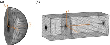
 $e/\sqrt {s}$ and the walls of the hole) with unitary flux through the whole. We implemented the problem on the geometry shown in figure 11(a) which is composed of
 \begin{equation} \left.\begin{gathered} \text{half-hole,}\ \left\{x_{\mu}\in ({-}1/2,1/2), y_{\mu}\in(0,e/(2\sqrt{s})), z_{\mu}\in({-}1/2,1/2) \right\},\\ \text{half-sphere,}\ \left\{\left(x_{\mu}^2+\left(y_{\mu}-e/(2\sqrt{s})\right)^2+z_{\mu}^2\right)\in(0,R^2)\right\}, \end{gathered}\right\} \end{equation}
with  $R \gg e/\sqrt {s}$ in order to recover the limits (2.7) (in practice,
 $R=10$). The boundary conditions applied to the boundaries of the computational domain are
 \begin{equation} \left.\begin{gathered} f=0,\quad \text{for}\ x_{\mu}\in ({-}1/2,1/2), y_{\mu}=0, z_{\mu} \in ({-}1/2,1/2),\\ {\boldsymbol{\nabla}} f\boldsymbol{\cdot} \boldsymbol{e}_{{\boldsymbol r}_{\mu}}=\frac{1}{2{\rm \pi} R^2},\quad \text{for } \sqrt{x_{\mu}^2+\left(y_{\mu}-e/(2\sqrt{s})\right)^2+z_{\mu}^2}=R,\quad y_{\mu}>e/(2\sqrt{s}). \end{gathered}\right\} \end{equation}
Once  $f$ has been computed, we deduce the blockage coefficient
 \begin{equation} b=2 \lim_{r_{\mu}\to \infty} \left(f({\boldsymbol r}_{\mu})+\frac{1}{2{\rm \pi} r_{\mu}}\right) \end{equation}
(in practice, for  $r_{\mu }=R$). This problem has been solved using Comsol Multiphysics.
(a) Geometry and mesh of the computational domain to solve the microscopic problem on  $f({\boldsymbol r}_{\mu })$. (b) Geometry and mesh of the computational domain to solve the eigenvalue problem (B5) on
 $\Phi _{per}({\boldsymbol r})$ (band diagram).

B.2. Band diagrams
The band diagram is obtained by solving the three-dimensional direct problem set on  $\varPhi ({\boldsymbol r})$, (3.1a,b)–(2.2a,b), in the unit cell shown in figure 11(b) (see also figure 4) with Bloch–Floquet decomposition
 \begin{equation} \varPhi({\boldsymbol r})=\Phi_{per}({\boldsymbol r})\exp({{\rm i}{\boldsymbol \kappa}\boldsymbol{\cdot} {\boldsymbol r}}), \end{equation}
where  $\Phi _{per}({\boldsymbol r})$ is a periodic function with periodicity
 $\ell _x$ along
 $x$, and
 $\ell _y$ along
 $y$, and with
 ${\boldsymbol \kappa }=\kappa _x\boldsymbol {e}_x+\kappa _x\boldsymbol {e}_y$. Numerically, we implemented the weak formulation of the eigenvalue problem for
 $\Phi _{per}({\boldsymbol r})$, i.e. set on a periodic cell
 $\varOmega _t$. It results that the resolution consists, for a given wavevector
 ${\boldsymbol \kappa }$, to find the set of
 $(\omega,\Phi _{per})$ such that for any (periodic) test function
 $\Phi _{per}^*$, we have
 \begin{align} & \int_{\varOmega_t}
(\boldsymbol{\nabla} \Phi_{per}
\boldsymbol{\cdot}\boldsymbol{\nabla} \Phi_{per}^*
+\kappa^2\, \Phi_{per}\Phi_{per}^*-{\rm
i}\,\Phi_{per}^*{\boldsymbol \kappa}
\boldsymbol{\cdot}\boldsymbol{\nabla} \Phi_{per} +{\rm
i}\Phi_{per}{\boldsymbol \kappa}
\boldsymbol{\cdot}\boldsymbol{\nabla}
\Phi_{per}^*)\text{d} \varOmega \nonumber\\ &\quad
-\int_{z=0} \frac{\omega^2}{g}\,\Phi_{per} \Phi_{per}^*
\,\text{d} S=0, \end{align}
where  $\kappa ^2={\boldsymbol \kappa }\boldsymbol {\cdot }{\boldsymbol \kappa }$. This problem has been solved using Comsol Multiphysics with the weak formulation PDE interface.
B.3. Numerical experiments with a source term
For the results reported in figures 8–10, the set of equations (3.1a,b)–(2.2a,b) has been modified to account for source terms, specifically
 \begin{equation} {\rm \Delta} \varPhi({\boldsymbol r})=S({\boldsymbol r}). \end{equation}
We define a elementary source as
 \begin{equation} s_e({\boldsymbol r})=\exp({-(x^2+y^2+z^2)/d^2}),\quad d=\ell_x/10. \end{equation}
The results reported in figures 8 and 9 have been obtained using a point source, and we imposed  $S({\boldsymbol r})=s_e({\boldsymbol r})$ with the computational domain being
 $\{x\in (-15\ell _y,15\ell _y),\ y\in (-15\ell _y,15\ell _y), z\in (-h,0)\}$.
The results on negative refraction (figure 10) involve an incident beam. In the numerics, we used
 \begin{equation} S({\boldsymbol r})=\sum_c s_e({\boldsymbol r}-{\boldsymbol r}_c), \end{equation}
with  ${\boldsymbol r}_c$ the centres of a hundred elementary sources located along a segment inclined at
 $45^\circ$ with respect to the
 $y$-axis (the segment is visible in figure 10).
In both cases, in order to avoid the reflection on the borders of the domain, we used perfectly matched layers of thickness  $2.5\ell _y$. These problems have been solved using the Matlab toolbox Pdetool (partial differential equations using finite element analysis).
Appendix C. Resonance frequency and blockage coefficient
In Euvé et al. (Reference Euvé, Pham, Petitjeans, Pagneux and Maurel2021a,Reference Euvé, Piesniewska, Maurel, Pham, Petitjeans and Pagneuxb), we pointed out the analogy between an underwater resonant cavity for water waves and an acoustic Helmholtz resonator in two dimensions. Here, the geometry of the cavity is three-dimensional, and we will see that, mutatis mutandis, the analogy still holds. The resonance frequency of a Helmholtz resonator, which applies to the acoustic pressure, is obtained by integrating the Helmholtz equation over the cavity and further by assuming that the acoustic velocity in the hole is constant. We repeat this exercise and integrate the incompressibility condition over the cavity, with  $\varphi _1$ the constant potential within the resonator, and
 $\varphi _{|N}$ the value of the potential at the exit of the neck. Accordingly, we obtain
 \begin{equation} 0=\int {{\rm div}}\, {\boldsymbol u} \,\text{d}{\boldsymbol r}=\frac{\omega^2S_c}{g}\,\varphi_1 +s\,v_{|N}, \end{equation}
with  $v_{|N}={\boldsymbol u}\boldsymbol {\cdot } {\boldsymbol n}$ at the exit of the resonator neck. Assuming as in the acoustic case that the velocity is constant in the neck of length
 $e$, we have
 $v_{|N}=(\varphi _{|N}-\varphi _1)/e$, hence
 \begin{equation} (\omega^2-\omega_r^2)\varphi_1={-}\omega_r^2\varphi_{|N},\quad \omega_r^2= \frac{s g}{e S_c}. \end{equation}
The above estimate of the resonance frequency does not account for boundary layer effects at the extremities of the hole, due to evanescent fields. This is what has been accounted for in § 2.2, where we analysed the potential flow through a hole, resulting in the resonance frequency  $\omega _0$ in (3.10a–c), with
 $\alpha =\sqrt {s}/b$ in (2.9). The blockage coefficient
 $b$, for a hole with unitary cross-section and length
 $e/\sqrt {s}$, depends only on the shape of the hole cross-section and on
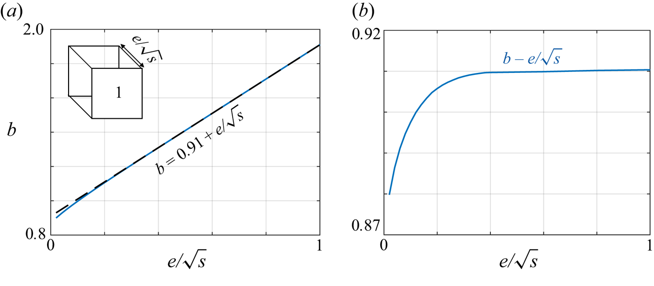
 $e/\sqrt {s}$. In figure 12, we report the variations of
 $b(e/\sqrt {s})$ calculated for square-shaped hole. Not surprisingly, we obtain
 $b\simeq b_0+e/\sqrt {s}$ (
 $b_0\simeq 0.91$), and the same result would be obtained for other shapes of hole cross-section (with a different value of
 $b_0$). Consequently, (3.10a–c), along with (2.9), provides
 \begin{equation} \omega_0^2={\frac{\alpha g}{S_c}}=\frac{s g}{(e+b_0\sqrt{s})S_c}, \end{equation}
with the hole length  $e$ in (C2) replaced by a so-called effective length
 $e_{eff}=e+b_0\sqrt {s}$. We notice in figure 12 that for
 $e/\sqrt {s}<1$, the blockage coefficient
 $b_0$ varies slightly because the effects of the evanescent fields at each end of the hole are no longer independent.
(a) Blockage coefficient  $b$ of a infinite wall pierced by a square hole with unitary cross-section and normalized length
 $e/\sqrt {s}$ (solid blue line); a good estimate is given by
 $b=b_0+e/\sqrt {s}$,
 $b_0=0.91$, (dashed black line). (b) Variation of
 $b-e/\sqrt {s}$, revealing a small shift with respect to the law
 $b=b_0+e/\sqrt {s}$ for vanishing
 $e$.

Appendix D. Rigid plates piercing the free surface
We report in this appendix a quick reminder on the strongly dispersive character of rigid plates piercing the free surface (figure 13a), introduced by Porter (Reference Porter2021) and Porter & Marangos (Reference Porter and Marangos2022), which we use as a reference case. To begin with, note that for subwavelength period, this three-dimensional configuration is the exact analogue of the two-dimensional acoustic case, i.e. the potential  $\varphi (x,y)\,f(z)$ exactly satisfies the Helmholtz equation
 \begin{equation} (\varDelta +k^2)\varphi=0,\quad k^2=\frac{\omega^2}{gh}, \end{equation}
because no evanescent mode is triggered. For a relative spacing  $\xi$ between the plates, the homogenized version of the dispersion is known (Mercier et al. Reference Mercier, Cordero, Félix, Ourir and Maurel2015; Marigo & Maurel Reference Marigo and Maurel2017) and takes the form
 \begin{equation} {{\rm div}}\,{\boldsymbol w} +\xi\,\frac{\omega^2}{g}\,\varphi=0,\quad {\boldsymbol w}=h\xi \boldsymbol{{R}}_{\alpha}\left(\begin{array}{cc} 1 & 0\\ 0 & 0 \end{array}\right) \boldsymbol{{R}}_{\alpha}^{{-}1}\,{\boldsymbol{\nabla}}\varphi, \end{equation}
where  $\boldsymbol{{R}}_{\alpha }$ is the rotation matrix of the angle
 $\alpha$. The search for a solution
 $\varphi (x,y)\propto \exp ({{\rm i}(\kappa _y x+\kappa _x y)})$ provides the dispersion
 \begin{equation} \cos\alpha \kappa_x+\sin\alpha \kappa_y={\pm} \frac{\omega}{\sqrt{gh}}, \end{equation}
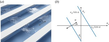
which gives isofrequency contours composed of two parallel lines (figure 13a). Therefore, the water wave energy is forced to follow the direction along the plates, as it should. As said previously, in the context of our study, the above dispersion for  $\alpha =0$ coincides with (1.1) for
 $\omega \gg \omega _0$ since from (3.13a,b) and (4.4a,b),
 $\chi _a\sim \chi _s\sim \varOmega ^2$, so
 $\kappa _x=\pm \kappa _0\varOmega =\pm \omega /\sqrt {gh}$.
(a) The case of arrays of inclined plates studied in Porter (Reference Porter2021) and Porter & Marangos (Reference Porter and Marangos2022). (b) Isofrequencycontour at constant  $\omega$ (where
 $\kappa _0=\omega /\sqrt {gh}$).

Appendix E. Dependence on the water depth
Here, we consider the possibility of taking into account the finite depth effect  $kh\sim 1$. To do so, we define the velocity potential
 \begin{equation} \psi(x,y,z)=\varphi(x,y)\,f(z),\quad f(z)=\cosh k(z+h), \end{equation}
which takes into account the dependence along  $z$ of the propagating mode, with the wavenumber
 $k$ now satisfying
 \begin{equation}w^2=g\,{\rm tanh}(kh).\end{equation}
For single-resonant canals, we proceed as in § 3. By integrating the incompressibility condition in the resonant cavity, we obtain
 \begin{equation} \frac{\omega^2S_c}{g}\,\frac{\cosh kh}{\cosh kh/2}\,\varphi_1 -\alpha(\varphi_1-\varphi)+\alpha(\varphi e_y-\varphi_1)=0 \end{equation}
(instead of (3.7)). We used the facts that the free surface condition applies to the potential at  $z=0$ and that the fluxes involve the potentials at depth
 $z^*=-h/2$. Integrating the incompressibility condition in the region of open canal in the unit cell, we obtain in the same way
 \begin{equation} S h\,F(h)\,\frac{\partial^2 \varphi}{\partial y ^2}+\frac{\omega^2S}{g}\,\frac{\cosh kh}{\cosh kh/2}\, \varphi-\alpha(\varphi-\varphi_1e_y^{{-}1})+\alpha(\varphi_1-\varphi)=0. \end{equation}
We used the fact that the integration in the open canal for  $z\in (-h,0)$ makes the integral
 $\int _{-h}^0 f(z)\,\text {d} z$ appear, thus
 \begin{equation} F(h)=\frac{\sinh kh}{kh \cosh kh/2}. \end{equation}
So we obtain the same relations as in (3.11) but with
 \begin{equation} \omega_0^2=\frac{\alpha g}{S_c}\,\frac{\cosh kh/2}{\cosh kh},\quad \kappa_0^2=\frac{\omega_0^2}{gh}\,\frac{kh}{2\sinh kh/2} \end{equation}
instead of (3.10a–c). Repeating the exercise for the doubly-resonant canals, we obtain the same relations as in (4.3) with again (E6a,b) instead of (3.10a–c). We note that  $\omega _0$ is now frequency-dependent, resulting in a lower resonance frequency; this is consistent with our observations (not reported) when, by increasing
 $h$, we leave the shallow-water regime. Another consequence is that the interpretation of
 $\kappa _0$ is no longer simple. The results are presented in figure 14; the branches for
 $\omega >5$ rad s
 $^{-1}$ where the dispersive effects become visible (see inset, which shows the deviation of
 $k$ from the shallow-water regime
 $\omega /\sqrt {gh}$) are well corrected when compared to the results in figures 5 and 6. We note, however, that the lower branches are also lightly shifted, which gives for
 $\gamma =1,2$ a slightly worse agreement for which we have no explanation.
Correction of the band diagrams accounting for a dependence of the potential on  $z$, (E1): (a) for single-resonant canals, to be compared with figure 4, and (b) for doubly-resonant canals, to be compared with figure 6. The inset in (a) for
 $\gamma =2$ shows the deviation of
 $k$ satisfying (??) with respect to the shallow-water prediction
 $k=\omega /\sqrt {gh}$.

Appendix F. Poynting vector
The derivation of the Poynting vector that enters the equation of energy balance requires that an effective model be available. The most classical model in the context in which we are interested is that of the stratified medium alternating open canals and surfacing piercing plates, which as said previously is the exact analogue of the acoustic problem. In this context, we have
 \begin{equation} \frac{\xi}{g}\,\ddot{\hat \varphi}({\boldsymbol x},t)-{{\rm div}}\,\hat{\boldsymbol w}({\boldsymbol x},t)=0,\quad \hat{\boldsymbol w}({\boldsymbol x},t)=\xi h\,\frac{\partial {\hat \varphi}}{\partial x}({\boldsymbol x},t)\,\boldsymbol{e}_x, \end{equation}
so  $\hat {w}_y=0$ (see e.g. Marigo & Maurel Reference Marigo and Maurel2017; Zhou Hagström, Maurel & Pham Reference Zhou Hagström, Maurel and Pham2021); the dot means the time derivative. We multiply the first equation by
 $\dot {\hat \varphi }$, and differentiate the second equation with respect to time and multiply it by
 ${\boldsymbol {\nabla }}\dot {\hat \varphi }$, then integrate the sum of the two contributions on a general surface
 $S$. We obtain
 \begin{equation} \frac{{\rm d}}{{\rm d} t}\int_S{\mathcal{E}}({\boldsymbol x},t)\,\text{d} s+\int_{\partial S}\hat{\boldsymbol {\rm \pi}}({\boldsymbol x},t)\,\text{d} l=0, \end{equation}
where the first term implies the local energy  ${\mathcal {E}}=\xi (\dot {\hat \varphi })^2/(2g)+\xi h(\partial _x{\hat \varphi })^2/2$, and the second term is the flux of the Poynting vector through
 $\partial S$, with
 $\hat {\boldsymbol {\rm \pi}}({\boldsymbol x},t)=-\dot {\hat \varphi }({\boldsymbol x},t)\,\hat {\boldsymbol w}({\boldsymbol x},t)$.
In the harmonic regime at the frequency  $\omega$, with
 ${\boldsymbol w}({\boldsymbol x},\omega ')={\boldsymbol w}({\boldsymbol x})\,\delta (\omega -\omega ')$, we have
 \begin{equation} \hat{\boldsymbol w}({\boldsymbol x},t)= 2\,{\rm Re}\left({\boldsymbol w}({\boldsymbol x})\exp({-{\rm i}\omega t})\right),\quad \dot {\hat \varphi}({\boldsymbol x},t)=2\,{\rm Im}\left(\omega\,\varphi({\boldsymbol x})\exp({-{\rm i}\omega t})\right). \end{equation}
which gives the expression of the Poynting vector averaged in time (on a period  $2{\rm \pi} /\omega$):
 \begin{equation} {\boldsymbol {\rm \pi}}({\boldsymbol x})=2\omega\,{\rm Im}\left(\varphi^*({\boldsymbol x})\,{\boldsymbol w}({\boldsymbol x})\right). \end{equation}
Using further that  ${\boldsymbol w}({\boldsymbol x})=\xi h\,\partial _x\varphi ({\boldsymbol x})\,\boldsymbol {e}_x$, and looking for a solution
 $\varphi ({\boldsymbol x})=\varphi \exp ({\rm i}(\kappa _x x+ \kappa _y y))$, we get
 \begin{equation} {\boldsymbol {\rm \pi}}({\boldsymbol x})=2\omega\,|\varphi|^2 \xi h \kappa_x \boldsymbol{e}_x. \end{equation}
As said in the main text, the analysis that provides (1.1) or (5.1) does not provide an effective model as (F1), mainly because the complexity of the system requires the use of the Bloch–Floquet analysis along  $y$. However, we can use the fact that (F1) is a particular limit of our resonant canal medium (above the resonances) to assume that (5.1) comes from an effective model of the form
 \begin{equation} \frac{\xi}{g_e}\,\omega^2\,\varphi({\boldsymbol x},\omega)+{{\rm div}}\, {\boldsymbol w}({\boldsymbol x},\omega) =0,\quad {\boldsymbol w}({\boldsymbol x},\omega)=\xi \left(\begin{array}{@{}cc@{}} h_x & 0\\ 0 & h_y \end{array}\right){\boldsymbol{\nabla}} \varphi({\boldsymbol x},\omega). \end{equation}
The form of the system (F6) provides (1.1) or equivalently (5.1) for a solution  $\varphi ({\boldsymbol x})=\varphi \exp ({{\rm i}(\kappa _x x+\kappa _y y)})$, and allows us to recover the limit (F1) in the time domain where
 $h_x=h$ and
 $h_y=0$ no longer depend on
 $\omega$. If this procedure is legitimate, then the balance of energy reads as in (F2), with a local energy
 ${\mathcal {E}}({\boldsymbol x},t)$ given by
 \begin{align} {\mathcal{E}} &= \xi\,\dot {\hat \varphi}({\boldsymbol x},t)\int_{-\infty}^\infty \frac{\ddot\varphi({\boldsymbol x},\omega)}{g_e(\omega)}\exp({-{\rm i}\omega t})\,\text{d} \omega \nonumber\\ &\quad +\frac{\hat{\boldsymbol w}({\boldsymbol x},t)}{\xi}\int_{-\infty}^\infty \left(\begin{array}{@{}cc@{}} h_x^{{-}1}{\omega} & 0\\ 0 & h_y^{{-}1}{\omega} \end{array}\right)\dot{\boldsymbol w}({\boldsymbol x},\omega)\exp({-{\rm i}\omega t})\,\text{d} \omega, \end{align}
while the expression of the Poynting vector in (F4) is still valid. With now  ${\boldsymbol w}(x)$ given by the second relation in (F6), and looking as before for a solution
 $\varphi ({\boldsymbol x})=\varphi \exp ({{\rm i}(\kappa _x x+\kappa _y y)})$, we obtain
 \begin{equation} {\boldsymbol {\rm \pi}}({\boldsymbol x})=2\omega \xi\,|\varphi|^2 (h_x \kappa_x+h_y \kappa_y), \end{equation}
as announced in (5.4).