1. Introduction
Wave propagation in an inhomogeneous ocean is one of the important and topical problems of physical oceanography and fluid mechanics, in general. However, it is a difficult problem from the mathematical point of view in the general statement due to the nonlinearity, dispersion and strong inhomogeneity. Analytical solutions either in the exact or approximate forms are possible in exceptional cases; see e.g. Stoker (Reference Stoker1957) and Sretensky (Reference Sretensky1977) in application to water waves. In these books, exact solutions for small-amplitude surface waves on water of arbitrary depth with a sloping bottom are presented. When the characteristic length of a small-amplitude wave is short in comparison with the typical scale of inhomogeneity, the well-known WKB (Wentzel–Kramers–Brillouin) approximation can be used for the description of quasi-monochromatic waves. However, in some special cases of variation of the parameters of the media, exact solutions can be derived for waves of arbitrary length both in the linear and even in the nonlinear cases. There is a vast volume of publications on this theme in the past two decades. Here we refer only to the most recent and relevant; others can be found in the cited publications (Didenkulova Reference Didenkulova2009; Didenkulova & Pelinovsky Reference Didenkulova and Pelinovsky2009; Didenkulova, Pelinovsky & Soomere Reference Didenkulova, Pelinovsky and Soomere2009; Dobrokhotov & Tirozzi Reference Dobrokhotov and Tirozzi2010; Grimshaw, Pelinovsky & Talipova Reference Grimshaw, Pelinovsky and Talipova2010b; Didenkulova & Pelinovsky Reference Didenkulova and Pelinovsky2011; Dobrokhotov, Nekrasov & Tirozzi Reference Dobrokhotov, Nekrasov and Tirozzi2011; Dobrokhotov, Medvedev & Minenkov Reference Dobrokhotov, Medvedev and Minenkov2013; Pelinovsky et al. Reference Pelinovsky, Didenkulova, Shurgalina and Aseeva2017a; Pelinovsky, Didenkulova & Shurgalina Reference Pelinovsky, Didenkulova and Shurgalina2017b; Pelinovsky et al. Reference Pelinovsky, Talipova, Didenkulova and Didenkulova2019). The outcomes of theoretical predictions for shallow-water waves were validated in the numerical modelling (see e.g. Vlasenko Reference Vlasenko1987; Choi et al. Reference Choi, Pelinovsky, Kim, Didenkulova and Woo2008; Pudjaprasetya, Risriani & Iryanto Reference Pudjaprasetya, Risriani and Iryanto2021). The important feature of such solutions is that they describe the reflectionless wave propagation when the wave energy is transmitted most effectively through the inhomogeneous zone without energy losses on wave reflection. Such situations can be the most dangerous from the point of view of their possible impact on ships and engineering constructions in coastal zones.
The problem of reflectionless wave propagation in inhomogeneous media has a long history. It was studied for monochromatic waves in plasma physics (Ginzburg Reference Ginzburg1970; Petrukhin, Pelinovsky & Didenkulova Reference Petrukhin, Pelinovsky and Didenkulova2020), acoustics (Brekhovskih Reference Brekhovskih1980), solids (Clements & Rogers Reference Clements and Rogers1974), fluids (Magaard Reference Magaard1962; Vlasenko Reference Vlasenko1987), etc. A more general analysis of reflectionless propagation of water waves of different shapes was presented in the above-cited papers by Didenkulova, Pelinovsky, Dobrokhotov et al. for particular configurations of bottom profile. In the cited publications, wave propagation was studied basically for a fluid without mean currents (in Dobrokhotov et al. (Reference Dobrokhotov, Medvedev and Minenkov2013), a particular case of a variable mean current was taken into account). However, in many cases, the influence of currents on wave propagation can be significant and, therefore, should be studied from the general point of view.
In this paper, we fill the gap and study in the long-wave approximation the reflectionless linear wave propagation in canals with variable depth, width and currents. The problem is formulated in terms of the velocity potential, which allows us to find the spatially varying mean flow profile, as well as the variation of the duct width and depth, that admit reflectionless wave propagation in ducts. We show that both global solutions defined on the entire  $x$-axis and bounded solutions defined only on the semi-infinite
 $x$-interval do exist, and we present particular examples. Then, we find the conditions that secure the existence of global solutions. The results obtained are illustrated graphically.
To solve this problem, we employ the transformation technique that has been used in many publications (see e.g. Grimshaw, Pelinovsky & Pelinovsky Reference Grimshaw, Pelinovsky and Pelinovsky2010a; Pelinovsky et al. Reference Pelinovsky, Didenkulova and Shurgalina2017b; and references therein). Such a technique is a particular case of the general methods of reduction of linear differential equations to some reference equations that can be solved analytically. These methods have developed starting back from the works of Euler, Laplace, Poisson, Darboux, et al., until now (see e.g. Bluman Reference Bluman1983; Varley & Semyr Reference Varley and Semyr1988; Chirkunov et al. Reference Chirkunov, Dobrokhotov, Medvedev and Minenkov2014; Kaptsov & Mirzaokhmedov Reference Kaptsov and Mirzaokhmedov2021; and references therein).
The paper is organised as follows. In § 2, we formulate the basic equations and derive the conditions under which wave propagation is reflectionless. The section ends with a simple condition that allows us to distinguish a particular class of global solutions. Then § 3 is devoted to the general analysis of the properties of solutions belonging to another class, among which there are both global and bounded solutions. Particular solutions of this class are obtained and analysed in § 4. In § 5, we explore the existence of smooth global solutions belonging to the second class and derive sufficient conditions for their existence. The possibility to construct global solutions by matching bounded solutions is considered in § 6. Finally, § 7 contains a discussion of results and concluding remarks. The technical aspects of matching solutions are considered in the Appendix.
2. Problem statement and general analysis
Let us consider the propagation of surface waves on a shallow-water flow in a duct with a width  $W(x)$ gradually varying along the direction of the flow with spatially varying depth
 $H(x)$ and bottom profile
 $z_B = B(x)$, as shown in figure 1 (note that the water surface is not horizontal in the presence of spatially inhomogeneous flow). In a stationary flow, the current velocity
 $U(x)$ is related to the duct parameters by the flux conservation law,
 \begin{equation} \varPhi \equiv U(x)H(x)W(x) = \mbox{const.}, \end{equation}
and the Bernoulli equation,
 \begin{equation} \tfrac{1}{2} U^{2}(x) + g [H(x) + B(x)] = \textrm{const}., \end{equation}
where  $g$ is the acceleration due to gravity. It is easy to see that, by appropriately choosing profiles
 $B(x)$ and
 $W(x)$, one can provide the desired (and independent) variation along the canal of the flow velocity
 $U(x)$ and the speed of long waves
 $c(x) = \sqrt {gH(x)}$; these velocities are assumed to be positive everywhere.
Sketch of the flow configuration in the vertical plane.

In the shallow-water theory, the linearised Euler equation is
 \begin{equation} \frac{\partial\tilde{u}}{\partial t}+\frac{\partial(U\tilde{u})}{\partial x} ={-}g\frac{\partial\eta}{\partial x}, \end{equation}
where  $\tilde {u}(x,t)$ is the perturbation of the longitudinal component of fluid velocity, and
 $\eta (x,t)$ is the deviation of the free surface from the equilibrium state. Then the mass balance equation is
 \begin{equation} \frac{\partial S}{\partial t} + \frac{\partial}{\partial x} [S(U+\tilde{u})] = 0, \end{equation}
where  $S(x,t)=[H(x)+\eta (x,t)]W(x)$ is the part of the duct cross-section occupied by water. Linearising this equation with respect to small perturbations
 $\eta$ and
 $\tilde {u}$, and taking into account (2.1) with
 $\varPhi \ne 0$, we obtain
 \begin{equation} \frac{\partial\eta}{\partial t} + \frac{1}{W}\frac{\partial}{\partial x} [W(U \eta + H \tilde{u})] \equiv \frac{\partial\eta}{\partial t} + HU\frac{\partial}{\partial x} \left(\frac{\eta}{H} + \frac{\tilde{u}}{U}\right) = 0. \end{equation}
Introducing the velocity potential  $\varphi$ such that
 $\tilde {u} = \partial \varphi /\partial x$, we integrate the linearised Euler equation (2.3) and present
 $\eta$ in terms of
 $\varphi$. Then, the combination of (2.3) and (2.5) gives the equation describing propagation of long waves:
 \begin{equation} \left(\frac{\partial}{\partial t}+U\frac{\partial}{\partial x}-2U\frac{c'}{c}\right) \left(\frac{\partial\varphi}{\partial t}+U\frac{\partial\varphi}{\partial x} \right) = \frac{g}{W} \frac{\partial}{\partial x}\left(W H \frac{\partial\varphi}{\partial x}\right), \end{equation}
where the prime stands for the derivative with respect to  $x$. This equation remains valid in the limiting case when
 $U(x) \equiv 0$. Using (2.1) with
 $\varPhi \ne 0$, we rewrite it in the form
 \begin{equation} \left(\frac{\partial}{\partial t}+U\frac{\partial}{\partial x}-2U\frac{c'}{c}\right) \left(\frac{\partial\varphi}{\partial t}+U\frac{\partial\varphi}{\partial x}\right)= c^{2}U\frac{\partial}{\partial x}\left(\frac{1}{U}\frac{\partial\varphi}{\partial x}\right). \end{equation}
This equation represents a basis for our analysis presented below but it does not admit the direct transition to the limiting case  $U(x) \equiv 0$.
For what follows, it is convenient to present the velocity potential in the form  $\varphi (x,t) = a(x)\psi (x,t)$, where the ‘amplitude factor’
 $a(x)$ will be defined later. Such a well-known trick allows one to reduce a linear equation with variable coefficients to one of the reference equations (see e.g. Grimshaw et al. Reference Grimshaw, Pelinovsky and Pelinovsky2010a; Pelinovsky et al. Reference Pelinovsky, Didenkulova and Shurgalina2017b; and references therein). After substitution of the expression for
 $\varphi$ in (2.7), we arrive at the following equation for
 $\psi (x,t)$:
 \begin{align} &\frac{\partial^{2}\psi}{\partial t^{2}} + (U^{2}-c^{2})\,\frac{\partial^{2}\psi}{\partial x^{2}} + 2U\,\frac{\partial^{2}\psi}{\partial t\partial x} + 2U\left(\frac{a'}{a} - \frac{c'}{c}\right)\frac{\partial\psi}{\partial t}\nonumber\\ &\quad +\left[2(U^{2}-c^{2})\,\frac{a'}{a} + (U^{2}+c^{2})\,\frac{U'}{U} - 2U^{2}\frac{c'}{c}\right]\frac{\partial\psi}{\partial x} + Z(x)\psi = 0, \end{align}
where  $Z(x)$ is defined by the equation
 \begin{equation} a(x)\,Z(x) = (U^{2}-c^{2})a'' + a' [(U^{2}+c^{2})(\ln U)' - 2U^{2}(\ln c)']. \end{equation}
Let us consider such a class of fluid flows for which  $Z(x) \equiv 0$. Then, from (2.9) we obtain the exact differential equation for
 $a(x)$ as
 \begin{equation} {\textrm{d}} (\ln a') = {\textrm{d}}\left(\ln \frac{c^{2}U}{c^{2}-U^{2}}\right). \end{equation}
The first integral of this equation is
 \begin{equation} \frac{{\textrm{d}}a}{{\textrm{d}}\kern0.7pt x} = D\frac{c^{2}U}{c^{2}-U^{2}}, \end{equation}
where  $D$ is a constant of integration.
Let us consider now a model equation:
 \begin{equation} \left(\frac{\partial}{\partial t} + s_1(x)\,\frac{\partial}{\partial x} +F(x)\right) \left(\frac{\partial}{\partial t} + s_2(x)\,\frac{\partial}{\partial x}\right)f(x,t) = 0, \end{equation}
where  $s_1(x)$,
 $s_2(x)$ and
 $F(x)$ are as yet undefined functions. One of the solutions to this equation describes a travelling wave:
 \begin{equation} f(x,t) = f_1\left(t - \int\frac{{\textrm{d}}\kern0.7pt x}{s_2(x)}\right), \end{equation}
where  $f_1(z)$ is an arbitrary function. Expansion of (2.12) leads to
 \begin{align} &\frac{\partial^{2} f}{\partial t^{2}} + s_1(x)s_2(x)\,\frac{\partial^{2} f}{\partial x^{2}} + \left[s_1(x) + s_2(x)\right]\frac{\partial^{2} f}{\partial t\partial x}\nonumber\\ &\quad + F(x)\,\frac{\partial f}{\partial t} + [s_1(x)s'_2(x) + F(x)s_2(x)]\, \frac{\partial f}{\partial x} = 0. \end{align}
Let us compare this equation with (2.8) provided that  $Z(x) \equiv 0$ and that (2.11) holds. These equations are identical if we define functions
 $s_1(x)$,
 $s_2(x)$ and
 $F(x)$ such that
 $$\begin{gather} s_1(x)s_2(x) = U^{2}(x) - c^{2}(x), \quad s_1(x) + s_2(x) = 2U(x), \end{gather}$$
 $$\begin{gather}F(x) = 2U(x)\left(\frac{a'(x)}{a(x)} - \frac{c'(x)}{c(x)}\right) \end{gather}$$
and
 \begin{align} & s_1(x)s'_2(x) + F(x)s_2(x)\nonumber\\ &\quad = 2 [U^{2}(x) - c^{2}(x)]\,\frac{a'(x)}{a(x)} + [U^{2}(x) + c^{2}(x)]\,\frac{U'(x)}{U(x)} - 2U^{2}(x)\,\frac{c'(x)}{c(x)}. \end{align}
Equations (2.15) hold if either  $s_1 = U - c$,
 $s_2 = U + c$, or
 $s_1 = U + c$,
 $s_2 = U - c$. It is easy to see that in both these cases (2.17) yields (up to an unimportant numerical factor)
 \begin{equation} a(x) = \left[c(x)U(x)\right]^{1/2}. \end{equation}
Using this relation, we can rewrite (2.11) in terms of functions  $c(x)$ and
 $U(x)$ (positive values of the roots
 $c^{1/2}(x)$ and
 $U^{1/2}(x)$ are presumed hereafter):
 \begin{equation} \frac{{\textrm{d}} (cU)}{{\textrm{d}}\kern0.7pt x} \equiv c(x)\,\frac{{\textrm{d}}U}{{\textrm{d}}\kern0.7pt x} + U(x)\,\frac{{\textrm{d}}c}{{\textrm{d}}\kern0.7pt x} = 2D\,\frac{c^{5/2}(x)\,U^{3/2}(x)}{c^{2}(x) - U^{2}(x)}. \end{equation}
Thus, when the relationships (2.15), (2.16), (2.18) and (2.11) hold, (2.7) can be presented in one of the following forms:
 \begin{align} &\left[\frac{\partial}{\partial t} + \left(U - c\right)\frac{\partial}{\partial x} + U\left(\frac{U'}{U} - \frac{c'}{c}\right)\right] \left[\frac{\partial}{\partial t}+ \left(U+c\right)\frac{\partial}{\partial x}\right]\psi \nonumber\\ &\quad \equiv \left[\frac{\partial}{\partial t} + \left(U + c\right)\,\frac{\partial}{\partial x} + U\left(\frac{U'}{U} - \frac{c'}{c}\right)\right] \left[\frac{\partial}{\partial t} + \left(U-c\right)\frac{\partial}{\partial x}\right]\psi = 0. \end{align}
The general solution of this equation can be presented as a superposition of two waves of arbitrary form travelling with different velocities:
 \begin{equation} \psi(x,t) = \psi_1\left(t-\int\frac{{\textrm{d}}\kern0.7pt x}{U(x)+c(x)}\right) + \psi_2\left(t-\int\frac{{\textrm{d}}\kern0.7pt x}{U(x)-c(x)}\right). \end{equation}
The independent propagation of each of these waves in an inhomogeneous fluid is provided by the single condition (2.11), which relates the fluid and wave speeds,  $U(x)$ and
 $c(x)$. Therefore, (2.11), when it holds, provides reflectionless (RL) wave propagation.
When the functions  $a(x)$ and
 $\psi (x, t)$ are found, then we get the velocity potential
 $\varphi$, which allows us to find the velocity
 $u$ and water surface elevation
 $\eta$:
 \begin{equation} \varphi(x,t) = a(x)\psi(x,t), \quad u = \frac{\partial\varphi}{\partial x}, \quad \eta ={-}\frac{1}{g}\left(\frac{\partial\varphi}{\partial t} + U\frac{\partial\varphi}{\partial x}\right). \end{equation}
A wide class of various RL flows can be obtained even in the simplest case when  $D = 0$. In such a case, (2.11) reduces to the condition
 $a(x) = \mbox {const.}$ or equivalently (see e.g. Churilov & Stepanyants Reference Churilov and Stepanyants2021)
 \begin{equation} c(x)U(x) = \mbox{const}. \end{equation}
The profile of one of these speeds can be specified as an arbitrary continuous positively defined function, and the profile of the other speed is uniquely calculated then. It is important to note that, firstly, such a flow is global, i.e. is defined on the entire  $x$-axis, and, secondly, neither the presence nor absence of critical points in the flow, at which the velocities
 $U(x)$ and
 $c(x)$ become equal, does not affect in any way such properties as smoothness and boundedness of the velocities.
3. Reflectionless flows in the case  $D \ne 0$: a general analysis

If  $D \ne 0$ is a positive or negative constant, singularities appear in the right-hand side of (2.19) when either
 $c = U$, or
 $U = 0$, or
 $c = 0$, and also when
 $U(x)$ or
 $c(x)$ grows with no limit when
 $x$ approaches some point
 $x_*$. If at least one of these singularities occurs at a finite point
 $x = x_*$, then several questions arise: (1) about the continuation of the flow model through this point; (2) about the contribution of the singular point to the wave reflection and/or absorption processes; and, more broadly, (3) about the existence of global RL flows. Below we investigate these issues.
We note first that (2.11) and (2.19) are invariant with respect to the simultaneous replacement  $x \to -x$ and
 $D \to -D$. For this reason, we introduce a variable
 $\xi = Dx$ which remains the same under such a transformation and rewrite (2.11) and (2.19) as
 \begin{equation} \frac{{\textrm{d}}a(\xi)}{{\textrm{d}}\xi} = \frac{c^{2}(\xi)U(\xi)}{c^{2}(\xi)-U^{2}(\xi)} \quad \textrm{and} \quad c(\xi)\frac{{\textrm{d}}U(\xi)}{{\textrm{d}}\xi} + U(\xi)\frac{{\textrm{d}}c(\xi)}{{\textrm{d}}\xi} = \frac{2c^{5/2}(\xi)U^{3/2}(\xi)}{c^{2}(\xi)-U^{2}(\xi)}. \end{equation}
In addition, (2.11), (2.19) and (3.1) are invariant with respect to the scaling transformation  $U(x) \to U(x)/c_s$ and
 $c(x) \to c(x)/c_s$, where
 $c_s = \mbox {const}$. In what follows, we will choose the appropriate scale
 $c_s$. Note also that these equations possess translational symmetry, which means that if
 $c(\xi )$ and
 $U(\xi )$ satisfy (3.1), then
 $c(\xi + b)$ and
 $U(\xi + b)$, where
 $b$ is an arbitrary constant, satisfy this equation too.
Let us introduce the dimensionless functions:  $u(\xi ) = w^{-1}(\xi ) = [U(\xi )/c(\xi )]^{1/2}$, noting that
 $c(\xi )u(\xi )=[c(\xi )U(\xi )]^{1/2}\equiv a(\xi )$. Then, let us rewrite (2.11) in the forms
 \begin{equation} \frac{{\textrm{d}}u}{{\textrm{d}}\xi} = \frac{u^{2}}{1-u^{4}} - \frac{u}{c(\xi)}\, \frac{{\textrm{d}}c(\xi)}{{\textrm{d}}\xi} \end{equation}
and
 \begin{equation} \frac{{\textrm{d}}}{{\textrm{d}}\xi}\ln a(\xi) = \frac{u(\xi)}{1-u^{4}(\xi)} = \frac{w^{3}(\xi)}{w^{4}(\xi)-1}. \end{equation}
The right-hand side of (3.3) is positive when  $u < 1$ (
 $w > 1$) and is negative when
 $u > 1$ (
 $w < 1$); therefore,
 $a(\xi )$ increases monotonically in subcritical flow and decreases monotonically in supercritical flow. If we assume that
 $c(\xi )$ is a bounded function at any finite
 $\xi$, i.e.
 $0 < c(\xi ) < \infty$, then the singularities at
 $U=0$ and
 $U=\infty$ can be reached only asymptotically when
 $\xi \to -\infty$. Similarly, under the assumption of the boundedness of
 $U(\xi )$, the singularities at
 $c = 0$ and
 $c = \infty$ can be reached only asymptotically when
 $\xi \to +\infty$. In all these cases, the right-hand side of (3.3) vanishes, hence the derivative in the left-hand side vanishes too. As the result of this, when
 $|\xi | \to \infty$, function
 $a(\xi )$ either asymptotically approaches some constant (which may be zero, in particular) or grows slower than an exponential function, e.g. in a power-type manner,
 $a(\xi )\sim |\xi |^{\alpha }$, where
 $\alpha >0$. In contrast to this, a singularity at
 $U=c$ (
 $u=w=1$) can be achieved (as will be shown below) at a finite point
 $\xi$.
To conclude this section, we consider the behaviour of the functions  $U(\xi )$ and
 $c(\xi )$ in the neighbourhood of a critical point where
 $U = c$. Assume that
 $\xi =0$ is a critical point, and the normalisation constant
 $c_s$ is chosen such that
 $U(0) = c(0) = 1$. Let us set
 \begin{equation} c(\xi) = 1 + s(\xi), \quad U(\xi) = 1 + v(\xi), \end{equation}
where  $s(\xi )\to 0$ and
 $v(\xi )\to 0$ when
 $\xi \to 0$. After substitution in the second equation of (3.1), we obtain
 \begin{equation} (s - v) (s' + v') = 1 + 2s + v + O(s^{2} + v^{2}), \end{equation}
where the prime stands for the derivative with respect to  $\xi$. From here, we see that
 $(s-v)$ and
 $(s+v)$ are power-type functions of
 $\xi$:
 \begin{equation} (s - v) \sim \xi^{\alpha}, \quad (s + v) \sim \xi^{\beta}, \end{equation}
where  $\alpha + \beta = 1$, with
 $\alpha > 0$ and
 $\beta > 0$.
Since  $\xi =0$ is a branching point and
 $s(\xi )$ and
 $v(\xi )$ are real functions, the cases
 $\xi >0$ and
 $\xi <0$ should be considered separately.
Case A. If  $\alpha =\beta =1/2$, then we readily find, for
 $\xi \geqslant 0$:
 \begin{equation} c(\xi) = 1+s_+\xi^{1/2}+O(\xi), \quad U(\xi) = 1+v_+\xi^{1/2}+O(\xi), \end{equation}
where  $s_+^{2} = v_+^{2} + 2$. For
 $\xi \leqslant 0$, we find:
 \begin{equation} c(\xi) = 1+s_-(-\xi)^{1/2}+O(\xi), \quad U(\xi) = 1+v_-(-\xi)^{1/2}+O(\xi), \end{equation}
where  $s_-^{2} = v_-^{2} - 2$. Here
 $s_\pm$ and
 $v_\pm$ are constants, which can have any sign, depending on the branch of the solution (subcritical or supercritical). Moreover, it is not necessary that both velocities have singularities at
 $\xi =0$. In particular, in the domain where
 $\xi \geqslant 0$, the flow velocity can be regular (
 $v_+=0$), while the wave velocity can be regular (
 $s_- =0$) in the domain where
 $\xi \leqslant 0$.
If  $\alpha \ne \beta$ then, we can present
 $s(x)$ and
 $u(x)$ as
 \begin{equation} s(\xi) = s_{a\pm} |\xi|^{\alpha} + s_{b\pm} |\xi|^{\beta} + \cdots, \quad v(\xi) = v_{a\pm} |\xi|^{\alpha} + v_{b\pm} |\xi|^{\beta} + \cdots, \end{equation}
where the indices plus (minus) pertain to the regions  $\xi \geqslant 0$ (
 $\xi \leqslant 0$).
Case B. Consider the case when  $0<\alpha <\beta$, then from the condition
 $(s+v)\sim |\xi |^{\beta }$, we obtain:
 \begin{equation} s_{a\pm}+v_{a\pm} = 0,\quad 2\beta s_{a\pm}(s_{b\pm}+v_{b\pm}) ={\pm} 1. \end{equation}
Case C. In another case,  $\alpha >\beta >0$, from the condition
 $(s-v)\sim |\xi |^{\alpha }$, we obtain:
 \begin{equation} s_{b\pm} = v_{b\pm}, \quad 2\beta s_{b\pm}(s_{a\pm} - v_{a\pm}) ={\pm} 1. \end{equation}
Note that if  $\alpha \ne \beta$, then both velocities inevitably have a singularity at the point
 $\xi =0$.
4. Examples of reflectionless flows
4.1. Currents with a constant wave speed
As a first example, consider a current with a constant wave speed  $c(\xi )\equiv 1$. From (3.1) we find
 \begin{equation} \frac{U'(\xi)}{U^{3/2}(\xi)} [1-U^{2}(\xi)] = 2 \quad \Longrightarrow \quad U^{2}(\xi) + 3(\xi-\xi_0)U^{1/2}(\xi) + 3 = 0. \end{equation}
Using the substitution  $v(\xi ) = U^{1/2}(\xi )$, we arrive at the algebraic equation for
 $v$:
 \begin{equation} F(v) \equiv v^{4} + 3(\xi-\xi_0)v + 3 = 0. \end{equation}
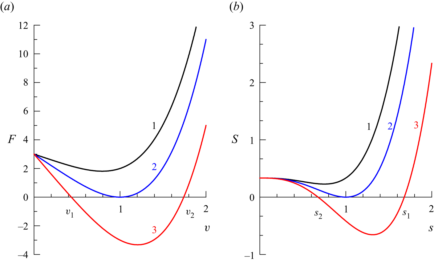
This equation has two positive real roots for  $\xi < \xi _* = \xi _0-4/3$, one of them being
 $v_1(\xi ) < 1$ and the other one
 $v_2(\xi ) > 1$ (see figure 2a). The roots merge into one double root
 $v=1$ (corresponding to the critical point where
 $U = c = 1$) when
 $\xi = \xi _*$. If
 $\xi > \xi _*$, then the polynomial (4.2) does not have positive roots. Without loss of generality, we can set
 $\xi _0 = 4/3$ (
 $\xi _* = 0$) bearing in mind that all the other solutions can be obtained by a shift in
 $\xi _0$. Then for
 $0 \leqslant -\xi \ll 1$ we have
 \begin{equation} v_{1,2}(\xi) = 1 \mp \left(-\frac{\xi}{2}\right)^{1/2}-\frac{\xi}{12} + \cdots, \quad U_{1,2}(\xi) = 1 \mp \left({-}2\xi\right)^{1/2} - \frac{2}{3}\,\xi + \cdots , \end{equation}
and for  $\xi \to -\infty$ the asymptotic solutions originated for each root are (recall that
 $a(\xi )=c(\xi )\,v(\xi )$):
 \begin{equation} \left.\begin{gathered} a_1(\xi) = v_1(\xi) \approx \left(4/3 - \xi\right)^{{-}1}, \quad a_2(\xi) = v_2(\xi) \approx \left(4 - 3\xi\right)^{1/3}, \\ U_1(\xi) \approx \left(4/3 - \xi\right)^{{-}2}, \quad U_2(\xi) \approx \left(4 - 3\xi\right)^{2/3}. \end{gathered}\right\} \end{equation}


The subcritical solution ( $U_1$) and supercritical solution (
 $U_2$) are defined only for the negative
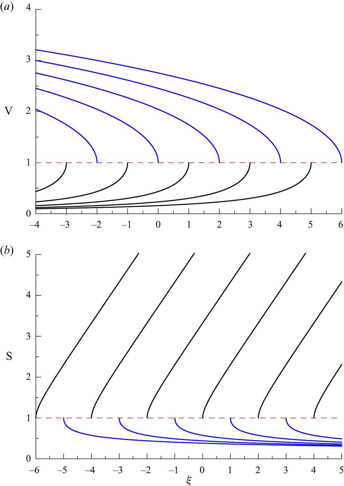
 $\xi \leqslant 0$. Profiles
 $v(\xi )$ are shown in figure 3(a) for different values of
 $\xi _0$. With the known dependences of
 $U_{1,2}(\xi )$ and fixed water depth
 $H_0$, we can calculate the dependences of the duct width
 $W(\xi )$ and bottom profile
 $z_B = B(\xi )$. Using (2.1) and (2.2), we obtain
 \begin{equation} W(\xi) \sim U^{{-}1}(\xi), \quad B(\xi) + \frac{1}{2g}U^{2}(\xi)={\rm const}. \end{equation}
(a) Solutions of (4.2) for different values of  $\xi _0$ in the subcritical (lower part of the panel) and supercritical (upper part of the panel) regions. (b) The same for the solutions of (4.7), but graphs for subcritical flows (
 $s>1$) are in the upper part of the panel, whereas graphs for supercritical flows (
 $s<1$) are in the lower part of the panel.

4.2. Currents with a constant flow speed
A very similar feature has a flow with a constant current speed,  $U(\xi )=1$. In this case (3.1) reduces to
 \begin{equation} \frac{c'(\xi)}{c^{5/2}(\xi)} [c^{2}(\xi)-1] = 2 \quad \Longrightarrow \quad c^{2}(\xi) - (\xi-\xi_0)c^{3/2}(\xi) + \frac{1}{3} = 0, \end{equation}
or equivalently to
 \begin{equation} S(s) \equiv s^{4} - (\xi-\xi_0)s^{3} + \frac{1}{3} = 0, \end{equation}
where  $s(\xi ) = c^{1/2}(\xi )$. There are two positive real roots for
 $\xi >\xi _* = \xi _0+4/3$,
 $s_1(\xi )>1$ and
 $s_2(\xi )<1$ corresponding to the subcritical and supercritical flows, respectively (see figure 2b). These roots merge at
 $s=1$ when
 $\xi = \xi _*$. The polynomial (4.7) does not have positive roots if
 $\xi < \xi _*$. Setting
 $\xi _0 = -4/3$ (
 $\xi _* = 0$), we find for
 $0\leqslant \xi \ll 1$:
 \begin{equation} s_{1,2}(\xi) = 1 \pm \left(\frac{\xi}{2}\right)^{1/2} + \frac{5}{12}\,\xi + \cdots, \quad c_{1,2}(\xi) = 1 \pm \left(2\xi\right)^{1/2} + \frac{4}{3}\,\xi + \cdots . \end{equation}
Then, for  $\xi \to +\infty$, we have (here
 $a(\xi )=s(\xi )U(\xi )$):
 \begin{equation} \left.\begin{gathered} a_1(\xi) = s_1(\xi) \approx \xi + 4/3, \quad a_2(\xi) = s_2(\xi) \approx \left(3\xi + 4\right)^{{-}1/3}, \\ c_1(\xi) \approx \left(\xi + 4/3\right)^{2}, \quad c_2(\xi) \approx \left(3\xi + 4\right)^{{-}2/3}. \end{gathered}\right\} \end{equation}
Note that, in contrast to the previous example, the solutions are defined only on the positive semi-axis  $\xi \geqslant 0$, because at
 $\xi =0$ the function
 $U(\xi )$ is regular. The profiles of
 $s(\xi )$ are shown in figure 3(b) for different values of
 $\xi _0$. From the known dependences of
 $c_{1,2}(\xi ) = \sqrt {gH(\xi )}$, we immediately derive the dependence of water depth
 $H_{1,2}(\xi ) = c^{2}_{1,2}(\xi )/g$. Then, from (2.1) with the fixed current flow
 $U_0$, we can calculate the dependences of the duct width
 $W(\xi )$ and bottom profile
 $z_B = B(\xi )$:
 \begin{equation} W(\xi) \sim H^{{-}1}(\xi) \sim c^{{-}2}(\xi), \quad B(\xi) ={-} H(\xi) +\mbox{const.} \end{equation}
In the next examples, we consider flows in which both velocities are unlimited in general.
4.3. Currents with functionally related velocity profiles
Consider now such class of fluid flows in which  $U(\xi )$ and
 $c(\xi )$ are related by the power-type equation:
 \begin{equation} U(\xi) = Vc^{p}(\xi), \quad V = \textrm{const.} > 0,\quad p = \textrm{const}. \end{equation}
We assume that  $p \ne \pm 1$. When
 $p=-1$, we arrive at the equation
 $c(x)U(x) = \mbox {const.}$, which corresponds to the case
 $D = 0$ (see the end of § 2). When
 $p=+1$, we obtain a flow with the constant Froude number,
 ${Fr} \equiv U(\xi )/c(\xi ) = V$, but with varying
 $c(\xi )$ and
 $U(\xi )$:
 \begin{equation} c(\xi) = C{\textrm{e}}^{\mu \xi}, \quad U(\xi) = Vc(\xi),\quad \mu = \frac{V^{1/2}}{1-V^{2}}. \end{equation}
As will be shown below, these are precisely such solutions that serve as the separatrices, separating solutions with fundamentally different behaviours.
Substituting  $U(\xi )$ from (4.11a–c) into (3.1) and integrating it, we obtain
 \begin{equation} \frac{2}{1-p}\,c^{(1-p)/2} + \frac{2V^{2}}{3(1-p)}\,c^{3(p-1)/2} = \frac{2V^{1/2}}{1+p}\left(\xi-\xi_0\right). \end{equation}
Introduction of the new variable  $u>0$, such that
 $u^{2} \equiv U/c = Vc^{p-1}$, yields
 \begin{equation} u^{4} + 3D_p(\xi-\xi_0)u + 3 = 0, \quad D_p=\frac{p-1}{p+1}. \end{equation}
In terms of the variable  $\zeta =D_p\xi$, this equation takes the same form as (4.2), and, therefore, its solutions are the same,
 $u_{1,2}(\zeta ) \equiv v_{1,2}(\zeta )$ (see figure 3a). All other variables
 $c$,
 $U$ and
 $a$ expressed in terms of
 $u$ are
 \begin{equation} c = c_*\,u^{{2}/({p-1})}, \quad U = u^{2} c = c_* u^{{2p}/({p-1})}, \quad a = u c = c_* u^{({p+1})/({p-1})}, \end{equation}
where  $c_*= V^{{1}/({1-p})}$ is the value of velocities at the critical point
 $\xi = \xi _*$,
 $U(\xi _*) = c(\xi _*) = c_*$. As one can see, the behaviour of these functions depends on the parameter
 $p$. Indeed, if we set
 $\zeta _0\equiv D_p\xi _0=4/3$, then we find with the help of (4.4) and (4.15a–c) that, when
 $\zeta \to -\infty$, the asymptotic behaviours of the functions of interest are
 \begin{align} \left.\begin{gathered}
c_1 \approx c_*\left(-\zeta\right)^{{2}/({1-p})}, \quad U_1
\approx c_*\left(-\zeta\right)^{{2p}/({1-p})}, \quad a_1
\approx c_*\left(-\zeta\right)^{({1+p})/({1-p})}, \\ c_2
\approx c_*\left(-3\zeta\right)^{{2}/(3(p-1))},
\quad U_2 \approx c_*\left(-3\zeta\right)^{{2p}/(3(p-1))},
\quad a_2 \approx c_*\left(-
3\zeta\right)^{({p+1})/(3(p-1))}.
\end{gathered}\right\} \end{align}
From these expressions we derive
 \begin{equation}
\left.\begin{array}{lll@{}} c_1, U_1, a_1 \to 0, & c_2, U_2,
a_2 \to \infty, & \textrm{for}\ p > 1,\\ c_1, U_1, a_1 \to
\infty, & c_2, U_2, a_2 \to 0, & \textrm{for}\ 0 < p < 1,\\
c_1, a_1 \to \infty, U_1 \to 0, & c_2, a_2 \to 0, U_2 \to
\infty, & \textrm{for}\ {-}1 < p <
0,\\ c_1 \to \infty, U_1, a_1 \to 0, & c_2 \to 0, U_2, a_2
\to \infty, & \textrm{for}\ p <{-}1.
\end{array}\right\}\end{equation}
In the neighbourhood of the critical point ( $\zeta \to 0_-$) we have
 \begin{align} c_{1,2}(\zeta) = c_*\left[1 \mp \frac{({-}2\zeta)^{1/2}}{p-1} + \cdots\right], \quad U_{1,2}(\zeta) = c_*\left[1 \mp \frac{p}{p-1}({-}2\zeta)^{1/2} + \cdots\right]. \end{align}
As an example, let us consider the flow in a duct of constant width  $W$. In accordance with the flux conservation law (2.1), such a flow corresponds to
 $p = -2$, and formulae (4.15a–c) yield
 \begin{equation} U(\xi) = c_* u^{4/3}(\xi), \quad c(\xi) = c_* u^{{-}2/3}(\xi), \quad H(\xi) = \frac{c^{2}_*}{g}\,u^{{-}4/3}(\xi). \end{equation}
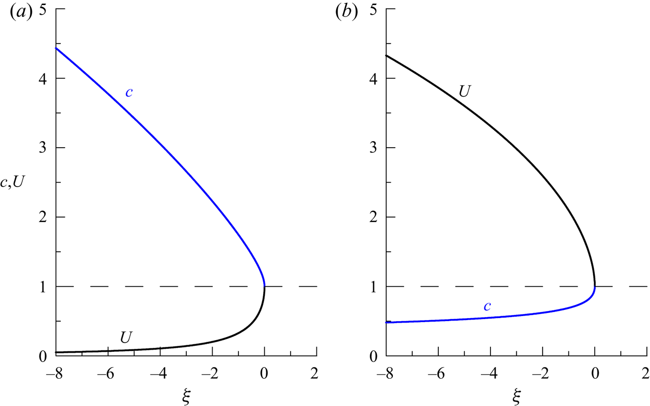
The profiles of velocities for  $\xi _* = 0$ and
 $c_*= 1$ are shown in figure 4.
The  $c(\xi )$ and
 $U(\xi )$ profiles of the RL flows in a duct of a constant width: (a) subcritical flow and (b) supercritical flow.

It should be noted that in all models with  $D \ne 0$ considered above, solutions are defined only on the semi-axis
 $\xi$, and the domains of their definition are limited because a singularity with
 $c = U$ occurs at a finite value of
 $\xi =\xi _*$. As the velocity
 $U(\xi _*) \ne 0$, it is evident that the flow goes over the point
 $\xi = \xi _*$ into the domain where
 $\xi > \xi _*$. One version of such flow models is discussed below in § 6.2.
4.4. Special class of flows with exponential variation of wave speed $c(\xi )$

The flows of this class differ significantly from those considered above. Let  $c(\xi ) = C\exp (\mu \xi )$. Then (3.2) takes the form
 \begin{equation} \frac{{\textrm{d}}u}{{\textrm{d}}\xi} = \frac{u^{2}}{1-u^{4}} - \mu u. \end{equation}
This equation, in contrast to that considered above, has a stationary point (the null isocline)  $u(\xi ) = u_0 = \mbox {const.}$ in which its right-hand side vanishes. The value of
 $u_0$ is a positive root of the following equation (cf. the last equation (4.12a–c), which reduces to (4.21) if we set
 $V = u_0^{2}$):
 \begin{equation} u_0^{4} + \frac{u_0}{\mu} - 1 = 0. \end{equation}
It is easy to see that, for  $\mu > 0$, the value of
 $u_0 < 1$, i.e. this corresponds to subcritical flows, whereas for
 $\mu < 0$, the value of
 $u_0 > 1$, which corresponds to supercritical flows.
Substituting  $u = u_0 + v$, where
 $|v| \ll u_0$, in (4.20), we obtain after linearisation with respect to
 $v$:
 \begin{equation} \frac{{\textrm{d}}v}{{\textrm{d}}\xi} = \left[\frac{2u_0}{1-u_0^{4}} + \frac{4u_0^{5}} {(1-u_0^{4})^{2}} - \mu\right]v = \mu(1 + 4\mu u_0^{3})v. \end{equation}
The solutions to this equation,
 \begin{equation} v(\xi) = v_0\exp(\gamma \xi), \quad \gamma = \mu(1 + 4\mu u_0^{3}), \quad v_0 = \mbox{const.}, \end{equation}
vanish when  $\xi \to -\infty$. This is obvious when
 $\mu > 0$ and, therefore,
 $\gamma > 0$. When
 $\mu < 0$, we obtain with the help of (4.21) that
 $\gamma$ is still positive:
 \begin{equation} \gamma = \mu [1 + 4(\mu/u_0 - 1)] = 4\mu^{2}/u_0 - 3\mu >0. \end{equation}
This means that the stationary point  $u_0$ is unstable owing to the fact that the small perturbation
 $v(\xi )$ grows with
 $\xi$.
As a result, the upper half-plane  $(\xi, u)$ is split into three strips (separated from each other by the straight lines
 $u = u_0$ and
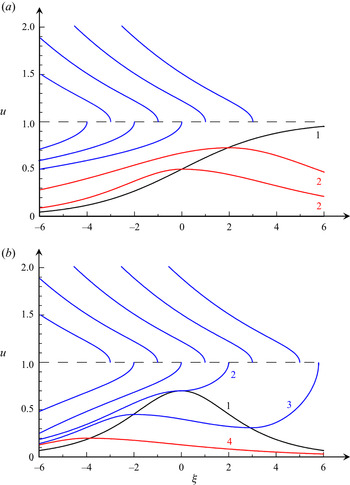
 $u = 1$), in which the behaviour of the solutions to (4.20) are significantly different (see figure 5).
Solutions of (4.20): panel (a) pertains to positive  $\mu =0.4$ (
 $u_0=0.3907$); and panel (b) pertains to negative
 $\mu =-0.4$ (
 $u_0=1.4705$). Global solutions are depicted by blue lines.

If  $\mu > 0$, then
 $0 < u_0 < 1$, and solutions to (4.20) are such as shown in figure 5(a). In the lower strip,
 $0 < u < u_0$, any solution
 $u(\xi )$ decreases monotonically, approaching
 $u_0$ from below when
 $\xi \to -\infty$ and
 $0$ from above when
 $\xi \to +\infty$, according to
 ${u \approx u_{m+}\exp (-\mu \xi )}$. Respectively, in the same limit, we have
 \begin{equation} U(\xi) \equiv u^{2}(\xi)\,c(\xi) \approx Cu^{2}_{m+}\textrm{e}^{-\mu\xi}, \quad a(\xi) = \left[c(\xi)\,U(\xi)\right]^{1/2} \to C u_{m+} = \textrm{const}. \end{equation}
In the middle strip,  $u_0 < u \leqslant 1$, any solution
 $u(\xi )$ grows monotonically from
 $u_0$ when
 $\xi \to -\infty$ to
 $u = 1$ at some
 $\xi _*$. Near this limiting coordinate
 $\xi _*$ the asymptotic solution is
 \begin{equation} u(\xi) = 1 - \left(\frac{\xi_* - \xi}{2}\right)^{1/2} - \frac{1 - 8\mu}{12}\left(\xi_* - \xi\right) + \cdots . \end{equation}
In the upper strip, any solution tends to infinity as  $u \approx u_{m-}\exp (-\mu \xi )$ when
 $\xi \to -\infty$ and decreases with
 $\xi$ approaching unity, when
 $\xi$ tends to some
 $\xi _+$ as per the formula:
 \begin{equation} u(\xi) = 1 + \left(\frac{\xi_+{-} \xi}{2}\right)^{1/2} - \frac{1 - 8\mu}{12}\left(\xi_+{-} \xi\right) + \cdots \end{equation}
If  $\mu < 0$, then
 $u_0 > 1$. The solutions to (4.20) are shown in figure 5(b). In the lower strip,
 $0 < u < 1$, all solutions
 $u(\xi )$ monotonically increase from
 $u\approx u_{M-}\exp (-\mu \xi )$ when
 $\xi \to -\infty$, attaining
 $u = 1$ at some finite
 $\xi$ according to the dependence similar to (4.26). In the middle strip,
 $1 < u < u_0$, solutions
 $u(\xi )$ monotonically decrease from
 $u_0$ when
 $\xi \to -\infty$ to
 $u = 1$, achieving this value at some finite
 $\xi$ as per the dependence similar to (4.27). In the upper strip,
 $u > u_0$, solutions
 $u(\xi )$ monotonically increase from
 $u_0$ when
 $\xi \to -\infty$, and to
 $u\approx u_{M+}\exp (-\mu \xi )$ when
 $\xi \to +\infty$; the dependences similar to (4.25a,b) hold in this limit.
It should be noted that in the lower strip for  $\mu > 0$ and in the upper strip for
 $\mu < 0$ solutions describing flows are global, i.e. they are defined on the entire
 $\xi$-axis; whereas in other strips, solutions are defined only to the left of some finite point
 $\xi _*$, which is different for each particular realisation.
5. Global solutions and conditions for their existence
As follows from the analysis presented above for the specific flow models, in the majority of cases the solutions for the RL current profile are applicable only in limited spatial intervals, because the profiles of the duct depth, width or current become either singular at certain points or diverge at infinity. Therefore, one of the important questions is whether it is possible to find such conditions when solutions for the profiles are globally defined on the entire  $x$-axis. Such a problem was solved in the case when there is no current (Pelinovsky et al. Reference Pelinovsky, Didenkulova and Shurgalina2017b). We provide the solution for the case when the current is taken into account.
Let us recall that in the case of the exponential variation of the wave speed  $c(\xi )$ considered above, the null isoclines are horizontal (
 $u_0 =\mbox {const.}$). Therefore, they serve as separatrices separating the global solutions from those that are defined on bounded
 $x$-intervals. Under a non-exponential variation of
 $c(\xi )$, the null isocline
 $u = u_0(\xi )$, on which the right-hand side of (3.2) vanishes, is still described by (4.21) but now
 \begin{equation} \mu(\xi) \equiv \frac{{\textrm{d}}}{{\textrm{d}} \xi}\ln{c(\xi)} \ne \mbox{const}. \end{equation}
Therefore, it is not horizontal and is intersected on the  $(\xi,u)$-plane by some solutions of (3.2). In what follows, we will assume that
 $c(\xi )$ either increases monotonically or decreases monotonically, determining accordingly the sign of
 $\mu (\xi ) \ne 0$. As follows from (3.2), when
 $\mu (\xi ) > 0$, then only subcritical solutions (
 $u(\xi ) < 1$) can be global; whereas when
 $\mu (\xi ) < 0$, only supercritical solutions (
 $u(\xi ) > 1$) can be global. Let us consider first flows with
 $\mu (\xi ) > 0$.
If the function  $c(\xi )$ grows faster than exponentially, then
 $\mu (\xi )$ monotonically increases with no limit (see figure 6a). The null isocline
 $u = u_0(\xi )$ also increases monotonically from zero when
 $\xi \to -\infty$ to unity when
 $\xi \to +\infty$ (see line 1 in figure 7a). The solutions of (3.2) either intersect the null isocline and are global, or lay entirely above it and are bounded from the right by some
 $\xi = \xi _b$. (Note that the null isocline has a positive derivative, whereas solutions below it have negative derivatives. Therefore, all such solutions intersect the null isocline when
 $\xi$ decreases.)
The qualitative dependence of  $\mu (\xi )$ for the flows in which
 $c(\xi )$ grows (a) faster than exponentially and (b) slower than exponentially.

Solutions of (3.2) in the case when  $c(\xi )$ grows (a) faster than exponentially and (b) slower than exponentially. Line 1 depicts the null isoclines in both panels. Lines 2 in panel (a) illustrate examples of global solutions; other unnumbered (blue) lines illustrate bounded solutions which exist for
 $\xi \leqslant \xi _b$ with the individual value of
 $\xi _b$ for each line. In panel (b) one can see several unnumbered (blue) lines depicting bounded solutions; line 2 depicts a solution tangent to the null isocline; line 3 is an
 $\xi$-bounded solution partially passing below the null isocline; and line 4 shows a global solution.

If the function  $c(\xi )$ grows slower than exponentially, then
 $\mu (\xi )$ has a maximum (possibly, even more than one, but it does not matter, in principle), vanishing when
 $\xi \to \pm \infty$ (see figure 6b). The null isocline
 $u = u_0(\xi )$ has qualitatively the same shape (see line 1 in figure 7b). All solutions lying above or crossing its right (descending) slope (for example, like line 3 in figure 7b) are, obviously, bounded from the right by some
 $\xi = \xi _b$. Let us consider now under what conditions global solutions such as shown by line 4 in figure 7(b) can exist.
Global solutions must be below  $u_0(\xi )$ for sufficiently large
 $\xi \geqslant \xi _M$. Let
 $\mu (\xi _M) \ll 1$, then, as follows from (4.21),
 $u_0(\xi ) \approx \mu (\xi ) \ll 1$ and it decreases with
 $\xi$ when
 $\xi \geqslant \xi _M$. Therefore, (3.2) simplifies and becomes
 \begin{equation} \frac{{\textrm{d}}u(\xi)}{{\textrm{d}}\xi} \approx u^{2}(\xi)-\mu(\xi)\,u(\xi) \equiv u^{2}(\xi) - \frac{u(\xi)}{c(\xi)}\,\frac{{\textrm{d}}c(\xi)}{{\textrm{d}}\xi}. \end{equation}
This equation reduces to
 \begin{equation} \frac{1}{(cu)^{2}}\,\frac{{\textrm{d}}}{{\textrm{d}}\xi}(cu) = \frac{1}{c(\xi)}, \end{equation}
and then can be readily solved:
 \begin{equation} \frac{1}{c(\xi)\,u(\xi)} = \frac{1}{c(\xi_M)\,u(\xi_M)} - \displaystyle\int\limits^{\infty}_{\xi_M}\frac{{\textrm{d}}y}{c(y)} + \displaystyle\int\limits^{\infty}_{\xi}\frac{{\textrm{d}}y}{c(y)}. \end{equation}
For the convergence of the integrals, the function  $c(\xi )$ must grow faster than linearly, for example, as
 $\xi ^{1 + \varepsilon }$ where
 $\varepsilon > 0$. Therefore, when
 $\xi \to +\infty$, then
 $c(\xi )u_0(\xi ) \approx c'(\xi ) \to +\infty$. Thus, the existence of global solutions is secured (i) by the convergence of the integrals in (5.4) and (ii) by the inequality
 \begin{equation} a_0^{{-}1} = \frac{1}{c(\xi_M)\,u(\xi_M)} - \displaystyle\int\limits^{\infty}_{\xi_M}\frac{{\textrm{d}}y}{c(y)} > 0. \end{equation}
The latter condition can be easily satisfied by the choice of sufficiently small  $u(\xi _M)$. As a result, on the solution that passes through the point
 $\left (\xi _M,u(\xi _M)\right )$, the product
 $c(\xi )u(\xi )$ goes to a finite limit
 $a_0 > 0$. Owing to this,
 $u(\xi ) < u_0(\xi )$ when
 $\xi \geqslant \xi _M$, i.e. this solution is global. Thus, global subcritical flows with
 $D \ne 0$ and smooth profiles
 $c(\xi )$ and
 $U(\xi )$ do exist under the conditions formulated above. Figure 8 demonstrates a qualitative variation of the flow parameters along the canal.
Qualitative dependences of typical variation of parameters in the case of a subcritical global flow along the canal. All variables are normalised to some reference values and presented in dimensionless form.

To study flows with  $\mu (\xi ) < 0$, it is convenient to use the variable
 $w(\xi ) = 1/u(\xi )$ (see (3.3) with
 $a(\xi ) = c(\xi )/w(\xi )$). In this case, all the reasoning presented above remains almost the same. In particular, if
 $c(\xi )$ decreases faster than exponentially, the null isocline and solutions on the half-plane
 $(\xi, w)$ look qualitatively the same as in figure 7(a) (with
 $u$ replaced by
 $w$). All solutions intersecting the null isocline are global, whereas those which do not intersect it are bounded on the right by some value
 $\xi _b$. If the function
 $c(\xi )$ decreases slower than exponentially, the solutions are similar to those shown in figure 7(b). For the existence of global solutions, it is sufficient that
 $c(\xi )$ decreases with
 $\xi$ as
 $\xi ^{-\varepsilon - 1/3}$ when
 $\xi \to +\infty$, and, for some point on the solution
 $\left (\xi _M, w (\xi _M)\right )$, where
 $\xi _M \gg 1$, the following inequality holds (cf. (5.5)):
 \begin{equation} a^{3}(\xi_M) \equiv \left[\frac{c(\xi_M)}{w(\xi_M)}\right]^{3} \equiv \left[c(\xi_M)u(\xi_M)\right]^{3} > \displaystyle\int\limits^{\infty}_{\xi_M}c^{3}(y)\,{\textrm{d}}y. \end{equation}
This inequality can be easily satisfied by the choice of a sufficiently small  $w(\xi _M)$ (large
 $u(\xi _M)$). In conclusion, we recall that, when
 $\mu (\xi ) < 0$, all global flows are supercritical (
 $U>c$).
6. Matching solutions for reflectionless flows
One can show that global solutions can exist only for rather artificial velocity profiles,  $c(\xi )$ and
 $U(\xi )$, whereas in the majority of cases these profiles are defined only on the semi-axis, either on the left or on the right of some point
 $\xi _*$. Using solutions for
 $D \ne 0$ defined on different sides of the selected common point, one can try to construct a global solution by matching two particular solutions. However, the matching procedure depends on the character of the common point, whether it is regular (
 $U \ne c$) or critical (where
 $U = c$). Below, we consider both these possibilities.
6.1. Matching solutions at the regular point
Let us assume that there are two solutions for the fluid flow satisfying (2.11): one of them describing velocities  $c_-(x)$ and
 $U_-(x)$ and defined for
 $x\leqslant x_m$, and the other solution describing velocities
 $c_+(x)$ and
 $U_+(x)$ and defined for
 $x\geqslant x_m$. Assume that
 $c_+(x_m)=c_-(x_m)=c_m$ and
 $U_+(x_m)=U_-(x_m)=U_m$, where
 $x=x_m$ is a regular point, i.e. such that
 $U_m\ne c_m$. As follows from (2.11), transition through the point
 $x=x_m$ is reflectionless if
 $D_+ = D_-$. If
 $D_+ \ne D_-$, then the function
 $a'(x)$ is discontinuous, and the coefficient
 $Z$ in (2.8) contains the term proportional to
 $Z\sim \delta (x-x_m)$, where
 $\delta (x)$ is the Dirac delta-function. In such a case, as will be shown in the Appendix, additional waves will appear on the left or right of point
 $x_m$.
To illustrate the possibility to construct a global solution, let us match two solutions at a regular point. To this end, we choose two solutions with equal constants  $D_\pm$ obeying equation (4.11a–c) for different parameters
 $p$ and
 $V$. In such a case, the profiles
 $c(\xi )$ and
 $U(\xi )$ depend on the same coordinate
 $\xi$. Let us set
 \begin{equation}
\left.\begin{array}{ccc@{}} c_-(\xi) = c_a(\xi), & U_-(\xi) =
U_a(\xi) = V_a c_a^{p_a}(\xi), & \xi \leqslant
\xi_m, \\ c_+(\xi) = c_b(\xi), &
U_+(\xi) = U_b(\xi) = V_b c_b^{p_b}(\xi), & \xi \geqslant
\xi_m, \\ c_a(\xi_m) = c_b(\xi_m), &
U_a(\xi_m) = U_b(\xi_m). & {} \end{array}\right\}
\end{equation}
Then, functions  $u_{a,b}(\xi ) = [U_{a,b}(\xi )/c_{a,b}(\xi )]^{1/2}$ satisfy equations similar to (4.14a,b):
 \begin{equation} u_{a,b}^{4} + 3D_{a,b}(\xi-\xi_{a,b})\,u_{a,b} + 3 = 0, \quad D_{a,b}=\frac{p_{a,b}-1}{p_{a,b}+1}. \end{equation}
The functions  $U_{a,b}(\xi )$ and
 $c_{a,b}(\xi )$ can be presented in terms of
 $u_{a,b}(\xi )$ using expressions similar to (4.15a–c). The existence of the functions
 $u_a(\xi )$ and
 $u_b(\xi )$, as well as the continuity of
 $u(\xi )$ (i.e.
 $u_a(\xi _m) = u_b(\xi _m) = u_m$) are secured by the following relations:
 \begin{equation} D_a(\xi_m - \xi_a) = D_b(\xi_m - \xi_b) <{-}\frac{4}{3}, \quad \left(\frac{V_a}{u_m^{2}}\right)^{p_b-1} = \left(\frac{V_b}{u_m^{2}}\right)^{p_a-1}. \end{equation}
For the resulting composite flow to be global, i.e. covering the entire  $\xi$-axis, the parameters
 $p_ {a, b}$ should be chosen such that
 $D_a$ and
 $D_b$ have different signs, namely,
 \begin{equation} D_a > 0 \quad\Longrightarrow\quad |p_a| > 1, \quad D_b < 0 \quad\Longrightarrow\quad |p_b| < 1. \end{equation}
It is important to remember that the value and sign of  $p$ significantly impact the behaviour of the functions
 $c(\xi )$ and
 $U(\xi )$ when
 $|\xi | \to \infty$ (see (4.16) and (4.17)). To find the profiles of the flow and wave velocities, in addition to
 $p_a$,
 $p_b$ and
 $\xi _m$, we must set, for example, the flow parameters
 $V_a$ and
 $\xi _a > \xi _m + 4/(3D_a)$ (see (6.3a,b)), select from the roots of (6.2a,b) the one that corresponds to the nature of the flow (subcritical or supercritical), and using (6.3a,b) find
 $V_b$ and
 $\xi _b$:
 \begin{equation} V_b = [u_m^{2(p_a-p_b)}\,V_a^{p_b-1}]^{{1}/({p_a-1})}, \quad \xi_b = \xi_m-\frac{D_a}{D_b}\left(\xi_m - \xi_a\right). \end{equation}
It should be emphasised that, with the exception of the trivial case  $p_a = p_b$, the velocity profiles have a kink at
 $x = x_m$, i.e. their derivatives are discontinuous. Indeed, calculating with the help of (4.15a–c) the logarithmic derivatives of
 $c(\xi )$ and
 $U(\xi )$, we find
 \begin{equation} \frac{c'_{a,b}}{c_{a,b}} = \frac{2}{p_{a,b}-1}\,\frac{u'_{a,b}}{u_{a,b}}, \quad \frac{U'_{a,b}}{U_{a,b}} = \frac{2p_{a,b}}{p_{a,b}-1}\,\frac{u'_{a,b}}{u_{a,b}}, \quad \left(\frac{a'(\xi)}{a(\xi)}\right)_{a,b} = \frac{p_{a,b}+1}{p_{a,b}-1}\,\frac{u'_{a,b}}{u_{a,b}}. \end{equation}
On the other hand, from (3.1) we get
 \begin{equation} \left(\frac{a'(\xi)}{a(\xi)}\right)_{a,b} = \frac{c_{a,b}^{3/2}\,U_{a,b}^{1/2}}{c_{a,b}^{2}-U_{a,b}^{2}} = \frac{u_{a,b}}{1-u_{a,b}^{4}}, \end{equation}
so that
 \begin{equation} \left(\frac{u'_{a,b}}{u_{a,b}}\right)_{\xi_m} = \frac{p_{a,b}-1}{p_{a,b}+1}\,\frac{u_m}{1-u_m^{4}} \equiv \frac{p_{a,b}-1}{p_{a,b}+1}\,\frac{(U_m/c_m)^{1/2}}{1-(U_m/c_m)^{2}} \end{equation}
and then
 \begin{align} \left(\frac{u'_b}{u_b} - \frac{u'_a}{u_a}\right)_{\xi_m} &= \left(\frac{U'_b}{U_b}-\frac{U'_a}{U_a}\right)_{\xi_m} ={-}\left(\frac{c'_b}{c_b}-\frac{c'_a}{c_a}\right)_{\xi_m}\nonumber\\ & = \frac{2(p_b-p_a)}{(1+p_a)(1+p_b)}\,\frac{(U_m/c_m)^{1/2}} {1-(U_m/c_m)^{2}} \ne 0. \end{align}
In figure 9 one can see the dependences  $u$,
 $c$ and
 $U$ on
 $\xi$ for two versions of matching of RL flows at the regular point (the velocities
 $c$ and
 $U$ are normalised to some reference values and presented in dimensionless form).
The result of matching of RL flow (4.11a–c) for different parameters: (a)  $p_a=5$,
 $V_a=1$,
 $p_b=1/5$; and (b)
 $p_a=-5$,
 $V_a=1$,
 $p_b=-1/5$. Solid lines pertain to subcritical flows (
 $U< c$), dashed line to supercritical flows (
 $U>c$).

6.2. Matching solutions at the critical point
Let us consider now the possibility of constructing a global solution by matching solutions with  $D \ne 0$ defined on different sides of a common critical point assuming that
 $c(\xi ) \equiv 1$. Let us set for certainty
 $\xi _0 = 4/3$ in (4.2); then the condition of no reflection (2.11) is satisfied only for
 $\xi < 0$, and a corresponding RL flow is defined only on this semi-axis. However, on the physical axis
 $x=\xi /D$ such a flow is defined for
 $x \leqslant 0$ if
 $D = D^{(-)} > 0$, and for
 $x \geqslant 0$ if
 $D = D^{(+)} < 0$. From these solutions defined on the different semi-axes, it is possible to construct a composite solution defined on the entire
 $x$-axis and describing the transition of subcritical flow into supercritical flow (see figure 10a), or supercritical flow to the subcritical flow (see figure 10b). If
 $D^{(+)}=-D^{(-)}$, then, given the asymptotic expansions (4.3a,b), the velocity profile
 $U(x)$ looks quite ‘smooth’ (if the infinite derivative at
 $x=0$ is ignored). The theory of wave propagation on shallow-water flows is well developed, including the cases when the current speed passes through the critical point having finite derivatives of the velocity profiles
 $U(x)$ and
 $c(x)$ (see e.g. Churilov, Ermakov & Stepanyants Reference Churilov, Ermakov and Stepanyants2017; Churilov & Stepanyants Reference Churilov and Stepanyants2021; and references therein). However, in the discussed case, a question about the contribution of the singular (sic!) point
 $x=0$ to the possible generation of additional waves still remains open. Potentially, some waves other than the incident and transmitted waves can emerge from the critical point. In addition, at least partial absorption of an incident wave can occur at the critical point.
Composite solutions of (4.2) describing the transition from (a) subcritical to supercritical flow and (b) in the opposite direction.

In a similar way, one can construct a matched solution for a flow with a constant velocity, with the only difference being that in this case the solution on the left ( $x\leqslant 0$) must have
 $D=D^{(-)} < 0$, whereas the solution on the right (
 $x\geqslant 0$) must have
 $D=D^{(+)} > 0$.
7. Conclusion
In this paper, we have shown that reflectionless (RL) propagation of long surface waves in a duct or in a channel with variable width  $W(x)$ and depth
 $H(x)$ in the presence of a spatially varying flow is quite possible if the velocities of the flow
 $U(x)$ and waves
 $c(x) = \sqrt {gH(x)}$ are interrelated by (2.19). It is important to emphasise that this single equation cannot define both functions
 $c(x)$ and
 $U(x)$ simultaneously. Therefore, it is necessary either to define one of them or set some additional relation between them. As a result, we arrive at two infinite classes of RL flows distinguished by whether or not the constant
 $D$ in (2.19) is equal to zero.
If  $D = 0$, the product
 $c(x)U(x)$ is constant along the canal (see condition (2.23)). All RL flows of this class have an interesting feature: the wider the canal, the higher the flow speed
 $U(x)$. Indeed, condition (2.23) is equivalent to
 $U(x) H^{1/2}(x) = \mbox {const}$. Then, from the flux conservation equation (2.1), it follows that
 $W(x) H^{1/2}(x) = \mbox {const.}$, so that
 $U(x) \sim W(x)$. Note that the same relation between the water depth and duct width was obtained by Pelinovsky et al. (Reference Pelinovsky, Didenkulova and Shurgalina2017b) to describe global RL solutions for the case when there is no current.
This class of RL flows has the advantage that we can attribute the  $x$-dependence arbitrarily to either of the two velocities
 $c(x)$ or
 $U(x)$, as well as the constant value to their product. Doing so, we can also attribute to
 $c(x)$ and
 $U(x)$ such important properties as continuity, differentiability, boundedness and so on. Moreover, we can define the flow on the entire
 $x$-axis, i.e. globally. As a result, the considered class contains currents with a wide variety of properties, including subcritical (
 $U < c$) and supercritical (
 $U > c$) flows, flows with transition from the subcritical to the supercritical regime and/or vice versa, as well as currents with other characteristics.
In contrast, when  $D \ne 0$, the properties of RL flows can vary in a much more restricted range. First of all, the currents of this class can be either subcritical or supercritical, because a transition through the critical point (where
 $U = c$) most likely violates the RL property of the flow. Secondly, the majority of RL flows are defined only on a certain interval of the
 $x$-axis, namely, on a ray bounded by the critical point
 $x_*$ at which
 $c(x_*) = U(x_*)$ (see § 4). Solutions are defined either on the right or on the left of
 $x_*$, depending on the parameters of the problem, e.g. on the sign of
 $D$.
In global flows of this class, as shown in § 5, the profiles of  $c(x)$ and
 $U (x)$ can be smooth functions of
 $x$ only if one of them, say
 $c(x)$, is varying (increasing or decreasing) fast enough. Global RL flows can also be constructed by matching bounded flows with equal values of
 $D$ and overlapping domains of definition at some regular point (where
 $c \ne U$) common to both flows. However, at this point the profiles of
 $c(x)$ and
 $U(x)$ necessarily have kinks (jumps in their derivatives – see § 6.1). With this in mind, one can construct a piecewise smooth flow by matching solutions many times at different points. Matching the currents with different values of
 $D$ is also possible, but this will inevitably lead to the occurrence of additional waves, i.e. to the loss of the RL property of the flow (see the Appendix).
The importance of the RL flows is that long surface waves of arbitrary form in the linear approximation can independently propagate in opposite directions of the  $x$-axis. This provides the most efficient energy transmission over a long distance through an inhomogeneous environment. The results obtained in this paper generalise earlier derived results (see Choi et al. Reference Choi, Pelinovsky, Kim, Didenkulova and Woo2008; Didenkulova Reference Didenkulova2009; Didenkulova & Pelinovsky Reference Didenkulova and Pelinovsky2009; Didenkulova et al. Reference Didenkulova, Pelinovsky and Soomere2009; Grimshaw et al. Reference Grimshaw, Pelinovsky and Pelinovsky2010a; Didenkulova & Pelinovsky Reference Didenkulova and Pelinovsky2011) for the cases when a water flow plays an important role and must be taken into consideration. However, we did not consider here two- or three-dimensional effects, which were studied to a degree in some of the cited papers. This interesting issue can be investigated elsewhere later. The results obtained can be of interest to mitigate the possible impact of waves on ships and marine engineering constructions in the coastal zones.
Funding
S.M.C. was financially supported by the Ministry of Science and Higher Education of the Russian Federation. Y.A.S. acknowledges the funding of this study provided by the Grant No. FSWE-2020-0007 through the State Task Programme in the Sphere of Scientific Activity of the Ministry of Science and Higher Education of the Russian Federation.
Declaration of interests
The authors report no conflict of interest.
Data availability statement
The data that support the findings of this study are available upon request from one of the authors (S.M.C.).
Author contributions
S.M.C. derived the theory. Both authors contributed equally to analysing the data and reaching conclusions, and in writing the paper.
Appendix A. Wave scattering at the matching point
In this Appendix, we show that, if  $D_+ \ne D_-$, then a composite flow will not be reflectionless. The ensemble of waves in the vicinity of the regular matching point is determined by whether the matching flows are subcritical (
 $U_m< c_m$) or supercritical (
 $U_m>c_m$). The solution of (2.8) obviously is continuous,
 $\psi _+(x_m,t) = \psi _-(x_m,t) \equiv \psi _m(t)$, and its time derivatives are continuous too. By integrating (2.8) over
 $x$ within the interval from
 $x_m-\varepsilon$ to
 $x_m+\varepsilon$ and denoting
 $[f] = f(x_m+\varepsilon )-f(x_m-\varepsilon )$ at
 $\varepsilon \to +0$, we obtain
 \begin{equation} \left[\frac{\partial\psi}{\partial x}\right] + \frac{1}{a_m}\left[\frac{\textrm{d}a}{{\textrm{d}}\kern0.7pt x}\right]\psi_m(t) = 0, \quad a_m = a(x_m) \equiv \left(c_mU_m\right)^{1/2}. \end{equation}
Using (2.11), we arrive at the matching conditions:
 \begin{equation} \left[\psi\right] = 0, \quad \left[\frac{\partial\psi}{\partial x}\right] + \frac{D_+{-}D_-}{c_m^{2}-U_m^{2}} \,a_m c_m\psi_m(t) = 0. \end{equation}
(i) Let us assume that the flows are subcritical in the vicinity of point  $x_m$ (
 $U_m < c_m$). Then the solution to the left of point
 $x_m$ can contain the incident and reflected waves, whereas the solution to the right of this point contains only a transmitted wave (see (2.21)):
 \begin{equation} \left.\begin{gathered} \psi_-(x,t) = \psi_1\left(t-\displaystyle\int\limits_{x_m}^{x}\frac{{\textrm{d}}z} {U_-(z)+c_-(z)}\right) + \psi_2\left(t+\displaystyle\int\limits_{x_m}^{x}\frac{{\textrm{d}}z}{c_-(z)-U_-(z)}\right),\\ \psi_+(x,t) = \psi_3\left(t-\displaystyle\int\limits_{x_m}^{x}\frac{{\textrm{d}}z} {U_+(z)+c_+(z)}\right). \end{gathered}\right\} \end{equation}
Matching these solutions in accordance with the conditions (A 2) leads to
 \begin{equation} \psi'_2(t) = \mu\left(\psi_1(t)+\psi_2(t)\right),\quad \mu = \frac{a_m}{2}\left(D_+{-} D_-\right). \end{equation}
Solving this equation under the assumption that the function  $\psi _1(t)$ vanishes sufficiently quickly when
 $t \to -\infty$, we derive
 \begin{equation} \psi_2(t) = \mu\displaystyle\int\limits_{-\infty}^{t}\psi_1(\tau)\,{\textrm{e}}^{\mu(t-\tau)}\,{\textrm{d}}\tau, \quad \psi_3(t)=\psi_1(t) + \psi_2(t). \end{equation}
It is easy to see that  $\psi _2(t) \equiv 0$ only if
 $\psi _1(t) \equiv 0$.
(ii) For the matching of supercritical flows ( $U_m > c_m$), we need to consider separately two cases.
If a wave of positive energy arrives from the left at the point  $x_m$, then we have
 \begin{equation} \left.\begin{gathered} \psi_-(x,t) = \psi_1\left(t-\displaystyle\int\limits_{x_m}^{x}\frac{{\textrm{d}}z} {U_-(z)+c_-(z)}\right),\\ \psi_+(x,t) = \psi_3\left(t-\displaystyle\int\limits_{x_m}^{x}\frac{{\textrm{d}}z} {U_+(z)+c_+(z)}\right) + \psi_4\left(t-\displaystyle\int\limits_{x_m}^{x}\frac{{\textrm{d}}z}{U_+(z)-c_+(z)}\right). \end{gathered}\right\} \end{equation}
Matching solutions at the point  $x_m$ leads to the equations
 $\psi '_4(t)+\mu \psi _1(t)=0$, so that we obtain
 \begin{equation} \psi_4(t) ={-}\mu\displaystyle\int\limits_{-\infty}^{t}\psi_1(\tau)\,{\textrm{d}}\tau, \quad \psi_3(t) = \psi_1(t) - \psi_4(t). \end{equation}
If a wave of negative energy (Fabrikant & Stepanyants Reference Fabrikant and Stepanyants1998) arrives from the left at the point  $x_m$, then we have
 \begin{equation} \left.\begin{gathered} \psi_-(x,t) = \psi_2\left(t-\displaystyle\int\limits_{x_m}^{x}\frac{{\textrm{d}}z} {U_-(z)-c_-(z)}\right),\\ \psi_+(x,t) = \psi_3\left(t-\displaystyle\int\limits_{x_m}^{x}\frac{{\textrm{d}}z} {U_+(z)+c_+(z)}\right) +\psi_4\left(t-\displaystyle\int\limits_{x_m}^{x}\frac{{\textrm{d}}z}{U_+(z)-c_+(z)}\right). \end{gathered}\right\} \end{equation}
Matching these solutions leads to the equation  $\psi '_3(t) = \mu \psi _2(t)$, so that we obtain
 \begin{equation} \psi_3(t) = \mu\displaystyle\int\limits_{-\infty}^{t}\psi_2(\tau)\,{\textrm{d}}\tau, \quad \psi_4(t) = \psi_2(t) - \psi_3(t). \end{equation}
Let us note in passing that if a superposition of waves with both positive and negative energies arrives from the left at the point  $x_m$,
 $\psi _- = \psi _1 + \psi _2$, then
 $$\begin{gather} \psi_3(t) = \psi_1(t) + \mu\displaystyle\int\limits_{-\infty}^{t}(\psi_1(\tau) +\psi_2(\tau))\,{\textrm{d}}\tau, \end{gather}$$
 $$\begin{gather}\psi_4(t) = \psi_2(t) - \mu\displaystyle\int\limits_{-\infty}^{t}(\psi_1(\tau) + \psi_2(\tau))\,{\textrm{d}}\tau. \end{gather}$$
Thus, we have seen that when  $D_+ \ne D_-$, the composite flow cannot be a RL flow in any regime, subcritical or supercritical.