1 Introduction
We consider the motion of a rigid body that adheres to a wall which is moving vertically upwards and is covered by a thin layer of viscous oil. When the wall is stationary the body remains attached to it by the oil and moves down the layer under the action of gravity.
The problem of a ball rolling down an inclined plane which is covered by a viscous layer has already been studied by Bico et al. (Reference Bico, Ashmore-Chakrabarty, McKinley and Stone2009). In the case where there is a vertical wall and there are collections of spheres, an interesting pattern formation is found (Kao & Hosoi Reference Kao and Hosoi2012). In this paper we consider the question of whether it is possible to balance the body on a vertically moving wall so that it is held at a fixed position.
In Eggers, Kerswell & Mullin (Reference Eggers, Kerswell and Mullin2013) observations were made using cylinders whose diameters are generally much larger than the thickness of the layer of oil. Extensive sets of results have been obtained using these bodies. As suggested above, it is possible to balance the bodies at a fixed position so that they rotate about a fixed horizontal axis with some of the fluid passing between the body and the wall and some being carried on the surface of the rotating cylinder.
In the present study we have decided to focus on the simpler configuration in which the bodies are cuboidal blocks which do not necessarily rotate about a horizontal axis. We describe the experiments in § 2 and in § 3 we develop a two-dimensional lubrication model which captures the salient features of the flow. The model gives good qualitative agreement with important flow features and reasonable quantitative agreement with observed wall speeds.
2 Experimental set-up
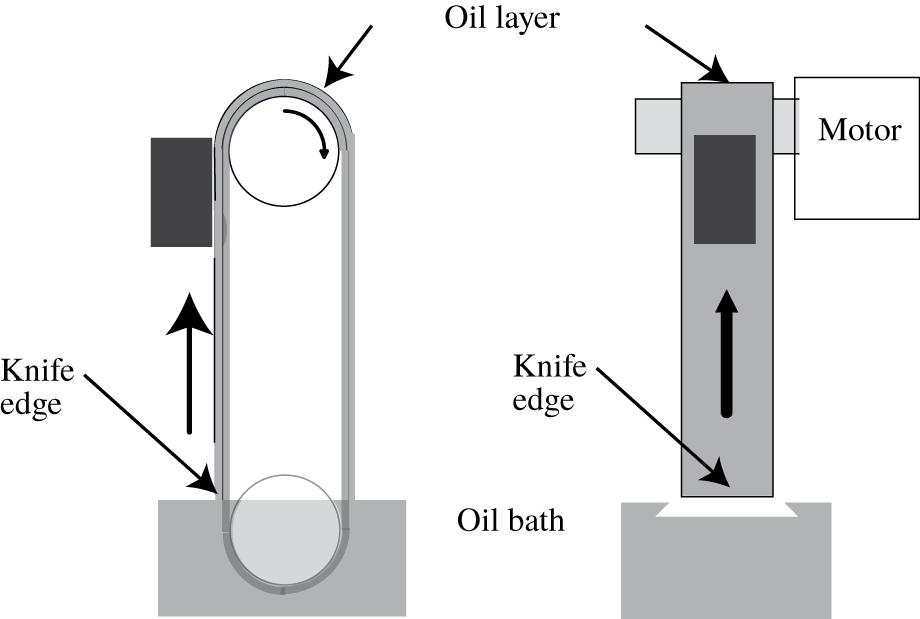
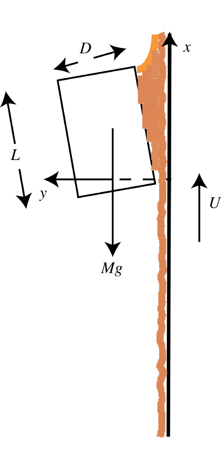
A schematic diagram of the experiment is given in figure 1 and a sketch of the flow under the block is given in figure 5. The smooth vertically moving surface was provided by the outside of a steel reinforced polyurethane engine timing belt which was 375 mm long and 26.5 mm wide. The section of belt which was used as the vertically moving wall was ∼150 mm long. The belt was driven by one of a pair of 38 mm toothed pulleys which were matched to the teeth on the inside of the belt. The drive was provided by a DC motor with controlled feedback loop which was connected to the drive pulley through a  $50:1$ gearbox. The rotation rate of the drive was monitored using an optical shaft encoder and a calibration between this and the belt speed was established and found to be linear. The output from the shaft encoder was displayed on a calibrated frequency counter and this provided a direct estimate of the speed of the belt.
Schematic diagram of the apparatus. Front and side views illustrating the position of the knife edge, fluid bath and drive cogs.

The fluid used in the experiments was silicone oil which had a measured dynamic viscosity of  $13\,341\pm 50.0~\text{cP}$ at
 $22\,^{\circ }\text{C}$. The experiments were performed in a temperature controlled environment where the temperature of the oil was measured to be
 $22\pm 0.5\,^{\circ }\text{C}$. The density of the silicone oil was
 $0.971\pm 0.001\times 10^{-3}~\text{g}~\text{cm}^{-3}$ and the surface tension 21.5 mN m-1. The low value of surface tension meant that the fluid readily wets the belt and enables the formation of a uniform layer. Other common viscous fluids such as glycerol and corn syrup have values of surface tension which are factors of two to three larger and hence they tend to form discrete patches of fluid on the belt. The belt passed through a bath of silicone oil and the thickness of the layer was set using a knife edge as a scraper fixed at a controlled distance from the belt. The thickness and uniformity of the layer were checked optically using a commercial confocal optical device from Microepsilon (confocalDT). The layer thickness was constant to within 10 % over the central area of the belt. Film drainage was not significant over the range of layer thicknesses used since the maximum drainage speed given by
 $u_{drain}=(gH_{k}^{2})/2\unicode[STIX]{x1D708}$ (where
 $g$ is gravitational acceleration,
 $H_{k}$ is the layer thickness and
 $\unicode[STIX]{x1D708}$ is the kinematic viscosity of the fluid) was an order of magnitude lower than the smallest belt speed. Hence drainage effects had negligible effect on variations in film thickness down the belt; nonetheless gravity effects are vital when considering the role of the fluid ‘tongue’ which usually forms beneath the block.
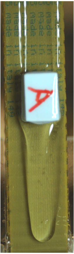
Polypropylene cuboid balanced on 0.5 mm layer at 4.718 mm s-1 which is ∼5 % above the theoretical belt velocity of 4.5 mm s-1 given by (3.17). The tongue is ∼1.5 mm thick at its centre.

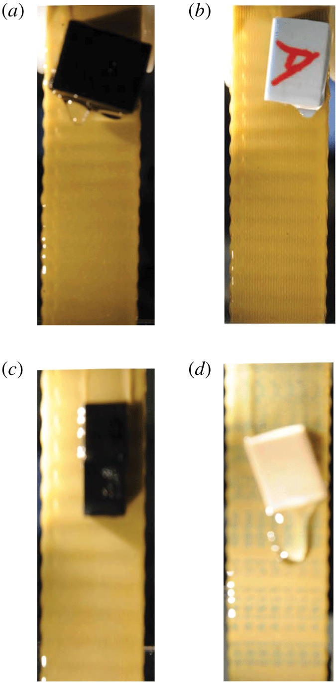
Four blocks balanced on layers 0.2 mm deep. The respective belt speeds were set to (a)  $4.80\pm 0.08~\text{mm}~\text{s}^{-1}$; (b)
 $7.01\pm 0.12~\text{mm}~\text{s}^{-1}$; (c)
 $2.66\pm 0.05~\text{mm}~\text{s}^{-1}$; and (d)
 $2.68\pm 0.05~\text{mm}~\text{s}^{-1}$. These values compare favourably with the values of
 $U^{\ast }$ defined in (3.17) namely,
 $4.48~\text{mm}~\text{s}^{-1}$,
 $6.53~\text{mm}~\text{s}^{-1}$,
 $3.09~\text{mm}~\text{s}^{-1}$ and
 $3.19~\text{mm}~\text{s}^{-1}$ respectively. Note that the blocks are typically slightly rotated with respect to the flow.

Experiments were performed with a number of blocks. The main results reported below were obtained using a  $20\times 10\times 10~\text{mm}^{3}$ printed plastic cuboid which had a density of
 $9\times 10^{-4}~\text{g}~\text{mm}^{-3}$. A set of observations were also obtained using a
 $10\times 10\times 10~\text{mm}^{3}$ printed plastic cube and polypropylene blocks with dimensions
 $19.25\times 13\times 13~\text{mm}^{3}$,
 $13.37\times 12.3\times 19.28~\text{mm}^{3}$ and
 $11.0\times 17.6\times 21.34~\text{mm}^{3}$. An example of a balanced state using this block is given in figure 2.
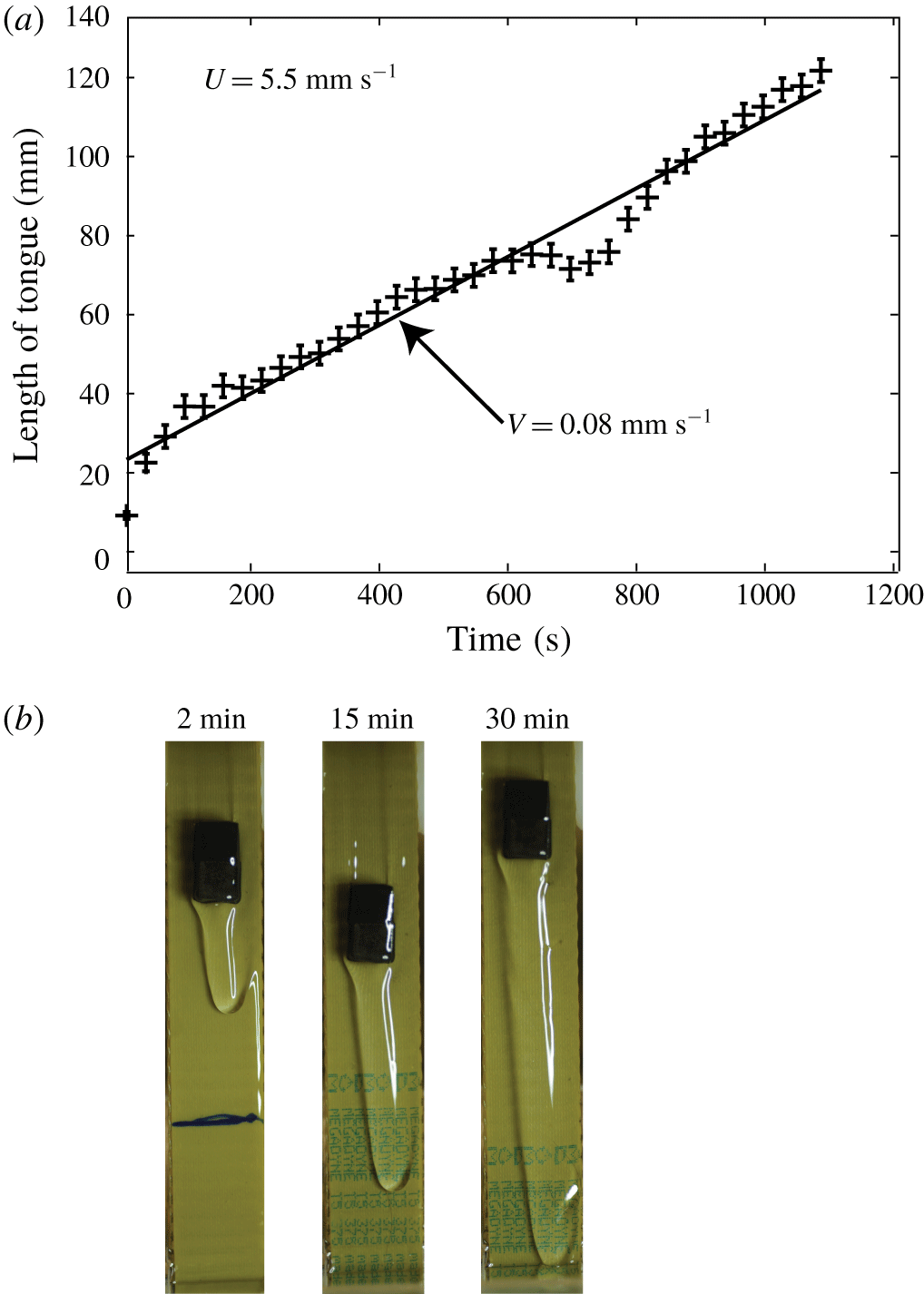
(a) Plot of distance travelled down the belt by the tongue versus time for  $20\times 10\times 10~\text{mm}$ cuboid on a 0.5 mm film. The speed of the belt was fixed at 5.5 mm s-1. N.B. Only data taken over the first 20 min are shown here. (b) Three images illustrating the tongue development at 5.5 mm s-1.

2.1 Experimental procedure
In all experiments the apparatus was run for an initial period of half an hour to establish a uniform film of viscous fluid on the belt. The thickness of the film was set using the knife edge. In earlier experiments with cylinders and spheres, achieving levitation was very straightforward in practice. This involved placing each levitating object on the moving layer and adjusting the speed of the belt to achieve balance. In these cases it was found that when the belt speed matched the fall speed of the sphere or cylinder, a balance was achieved. If the belt speed was too high, the levitating object moved up the belt, too low and it travelled downwards.
Levitating a rectangular block on the layer was considerably more challenging. The blocks were accurately machined pieces made primarily from plastic although a few results were obtained using metal cubes. If the block was simply placed on the belt it typically rotated about a horizontal axis perpendicular to the belt. However, if the block was held in tweezers until a small tongue of fluid developed, a steady levitated state could be achieved. If the belt speed was sufficiently high, the fluid tongue did not grow significantly. Determining the correct speed was an iterative procedure, so that obtaining a steady balanced state could take several hours. However, with due diligence we were able to levitate blocks, which ranged in shape from cubes to rectangular parallelepipeds, for many hours. It was initially difficult to obtain systematic results. A sample set of images of four different blocks levitated on a 0.2 mm layer is given in figure 3. In each case the tongue was very small and did not grow. However, the refined technique described in the following paragraph enabled the collection of reliable results for the growth of the tongue at lower belt speeds.
A systematic approach was developed which involved holding the block in a pair of tweezers with the lower face of the block immersed in the fluid layer as before. This produced a short tongue of fluid as in the left image in figure 4(b). This tongue then grew in length as in the next two images in figure 4. Once the tongue was established such that it was as long as the block, the block was released from the tweezers and this resulted in a levitating block which remained in situ for at least an hour. A practical limitation was that when the tongue reached the knife edge the incoming flow conditions changed. A further set of experiments was performed in which the speed of the belt was adjusted to investigate the growth rate of the tongue as a function of belt speed.
The tongue propagated slowly down the belt and typically took thirty minutes to an hour to reach the fluid bath. The speed of propagation of the tongue was estimated from still images which were captured every 30 s using a Nikon D400 SLR camera. Data used to estimate the tongue propagation speed were only taken in the period before the tongue reached the bath. A typical set of results for the tongue propagation are shown in figure 4(a) and three illustrative examples of the tongue development are shown in figure 4(b). In this case a  $20\times 10\times 10~\text{mm}$ cuboid was levitated on a 0.5 mm film and the belt speed was set at
 $5.5~\text{mm}~\text{s}^{-1}$. It can be seen that a straight line fits the data in figure 4(a) reasonably well. There is a clear departure from this for a short period and this arose when the block moved a small distance up the belt.
An important observation was that, in situations where small bubbles appeared on the free surface of the tongue, the bubbles always moved down from the block to the tip of the tongue.
3 A lubrication model
As mentioned in the Introduction, lubrication theory has already been used in Eggers et al. (Reference Eggers, Kerswell and Mullin2013) to model the levitation of a horizontal circular cylinder, a configuration that involves finding the extent of the lubrication region between the cylinder and the belt. The situation is simplified when a cuboidal block is levitated as in figure 2 because the stresses on the face of the block can be assumed to act over the whole face of the block as observed in the experiments in § 2. These stresses need to balance both the weight of the block denoted by  $Mg$ and its moment.
Assuming a stationary block, we will consider a two-dimensional model for the flow in figure 2, first for the flow between the block and the belt and then for the flow between the knife edge and the base of the block.
A schematic diagram of the flow in the lubrication layer between the block and the wall.

3.1 Flow between the block and the belt
Lubrication theory can be applied to the fluid flowing between the belt  $y=0$ and the block
 $y=H(x)=H_{0}(1+(mx/L))$ where
 $H_{0}$ and
 $m$ are to be determined. We assume that
 $H$ is comparable to the aperture at the knife-edge
 $H_{k}$, and
 $H_{k}/L=\unicode[STIX]{x1D6FF}$ is small, where
 $L$ is the length of the block in the direction of motion of the belt. The reduced Reynolds number is of
 $O(10^{-4})$ so that, to lowest order in
 $\unicode[STIX]{x1D6FF}$, the lubrication equations (Ockendon & Ockendon Reference Ockendon and Ockendon1995) for
 $p$, the pressure relative to atmospheric, and the velocity
 $(u,v)$ are
 $$\begin{eqnarray}\displaystyle & \displaystyle 0=-\frac{\unicode[STIX]{x2202}p}{\unicode[STIX]{x2202}x}-\unicode[STIX]{x1D70C}g+\unicode[STIX]{x1D707}\frac{\unicode[STIX]{x2202}^{2}u}{\unicode[STIX]{x2202}y^{2}}, & \displaystyle\end{eqnarray}$$
 $$\begin{eqnarray}\displaystyle & \displaystyle 0=\frac{\unicode[STIX]{x2202}p}{\unicode[STIX]{x2202}y}, & \displaystyle\end{eqnarray}$$
and
 $$\begin{eqnarray}0=\frac{\unicode[STIX]{x2202}u}{\unicode[STIX]{x2202}x}+\frac{\unicode[STIX]{x2202}v}{\unicode[STIX]{x2202}y},\end{eqnarray}$$
with
 $$\begin{eqnarray}u=U,v=0\quad \text{on }y=0\end{eqnarray}$$
and
 $$\begin{eqnarray}u=v=0\quad \text{on }y=H(x).\end{eqnarray}$$
We assume that  $p$ at the top corner of the block is zero to lowest order. This assumption will be discussed later when we will see that the pressures at
 $x=0$ and
 $x=L$ are both small, but the former is an order of magnitude greater than the latter. Hence, without loss of generality,
 $$\begin{eqnarray}p=0\quad \text{at }x=L.\end{eqnarray}$$
Equations (3.1)–(3.5) give that
 $$\begin{eqnarray}u=\frac{1}{2\unicode[STIX]{x1D707}}\left(\frac{\text{d}p}{\text{d}x}+\unicode[STIX]{x1D70C}g\right)y(y-H)+U\left(1-\frac{y}{H}\right),\end{eqnarray}$$
and  $p$ satisfies
 $$\begin{eqnarray}-\frac{1}{12\unicode[STIX]{x1D707}}\left(\frac{\text{d}p}{\text{d}x}+\unicode[STIX]{x1D70C}g\right)H^{3}+\frac{1}{2}UH=Q_{b},\end{eqnarray}$$
where  $Q_{b}$ is the constant flux per unit width between the block and the belt. Hence, from (3.6), (3.8),
 $$\begin{eqnarray}p=(L-x)\left[\unicode[STIX]{x1D70C}g+\frac{6Q_{b}\unicode[STIX]{x1D707}\left(2+m\left(1+{\displaystyle \frac{x}{L}}\right)\right)}{H_{0}^{3}\left(1+{\displaystyle \frac{mx}{L}}\right)^{2}(1+m)^{2}}-\frac{6\unicode[STIX]{x1D707}U}{H_{0}^{2}\left(1+{\displaystyle \frac{mx}{L}}\right)(1+m)}\right].\end{eqnarray}$$
The equations for the equilibrium of the block are, to first order in  $\unicode[STIX]{x1D6FF}$
 $$\begin{eqnarray}\displaystyle & \displaystyle \text{horizontal force balance: }\int _{0}^{L}p\,\text{d}x=0, & \displaystyle\end{eqnarray}$$
 $$\begin{eqnarray}\displaystyle & \displaystyle \text{vertical force balance: }W\int _{0}^{L}\left(p\frac{H_{0}m}{L}+\unicode[STIX]{x1D707}\frac{\unicode[STIX]{x2202}u}{\unicode[STIX]{x2202}y}\right)_{y=H}\,\text{d}x=-Mg, & \displaystyle\end{eqnarray}$$
 $$\begin{eqnarray}\displaystyle & \displaystyle \text{torque balance: }W\int _{0}^{L}xp\,\text{d}x=-{\textstyle \frac{1}{2}}MgD, & \displaystyle\end{eqnarray}$$
where  $D$ is the width of the block as shown in figure 5 and
 $W$ is its width in the third dimension. Thus we have three transcendental equations for
 $Q_{b}$,
 $H_{0}$ and
 $m$. When we neglect the right-hand side of (3.12) and the gravity term in (3.1), which is reasonable for the block sizes considered here, algebraic manipulations reveal that the only real solution is
 $$\begin{eqnarray}p=0,\quad m=0,\quad Q_{b}=\frac{\unicode[STIX]{x1D707}U^{2}LW}{2Mg},\quad H_{0}=\frac{\unicode[STIX]{x1D707}ULW}{Mg}.\end{eqnarray}$$
Thus, to lowest order in  $\unicode[STIX]{x1D6FF}$, the pressure is zero and the block is parallel to the wall in figure 5. Moreover, the flow under the block is a simple shear.
In standard lubrication theory the pressure is  $O(\unicode[STIX]{x1D707}U/L\unicode[STIX]{x1D6FF}^{2})$ and the inclination of the block is
 $O(\unicode[STIX]{x1D6FF})$ but here the right-hand side of (3.12) means that both of these estimates are multiplied by
 $\unicode[STIX]{x1D6FF}$. This can be seen by reference to the dimensionless form of the problem in appendix A, which also contains the corresponding lowest-order correction to (3.13). The calculation reveals that the pressure at
 $x=0$ takes the positive value
 $(6MgD)/(WL^{2})$, the implications of which will be discussed in § 3.3.
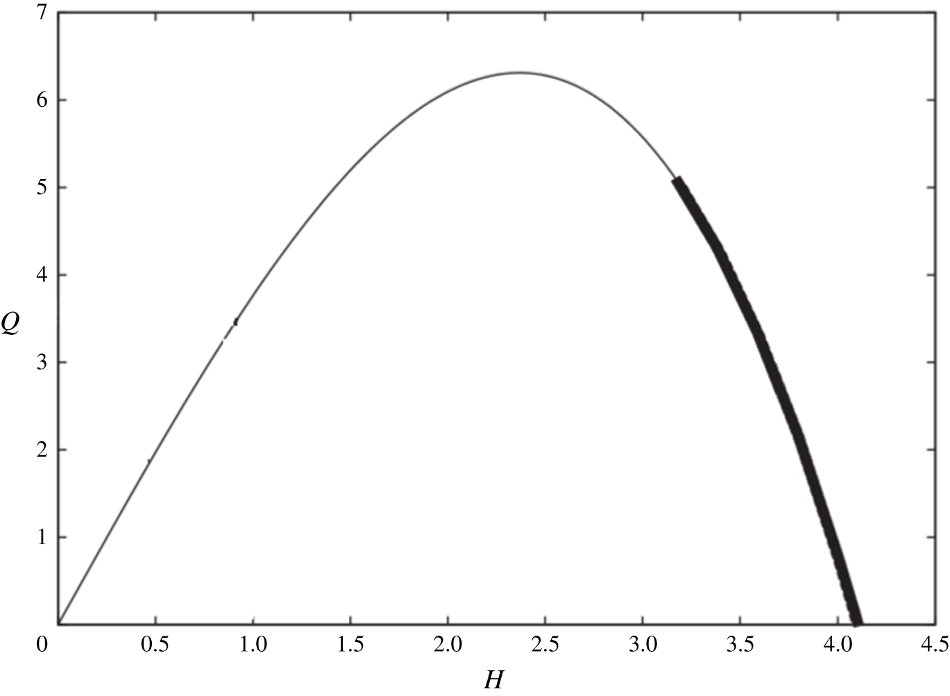
Relationship between  $Q$ and
 $H$ for the selected value of
 $U=4.0~\text{mm}~\text{s}^{-1}$ using (3.16). The heavy curve is for
 $UH>3Q$ and indicates the range of
 $H$ over which recirculating flow exists.

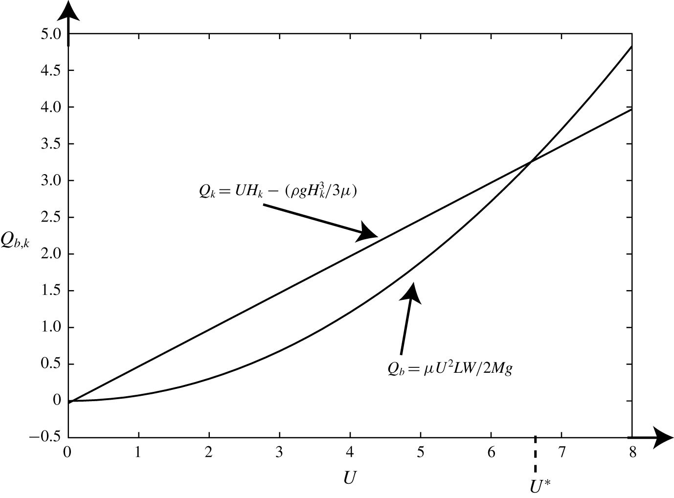
Plot of  $Q_{b}$ and
 $Q_{k}$ against
 $U$;
 $U^{\ast }$, the value of
 $U$ at which
 $Q_{b}=Q_{k}$, is indicated.

3.2 Flow between the block and the knife
The lubrication model (3.1)–(3.4) also applies to the region with a free surface below the block but (3.5) is replaced by
 $$\begin{eqnarray}p=0,\quad \frac{\unicode[STIX]{x2202}u}{\unicode[STIX]{x2202}y}=0\quad \text{on }y=H.\end{eqnarray}$$
Hence,  $p\equiv 0$,
 $H=\text{const.}$ and
 $$\begin{eqnarray}u=U+\frac{\unicode[STIX]{x1D70C}g}{2\unicode[STIX]{x1D707}}y(y-2H),\end{eqnarray}$$
so that the constant flux  $Q$ satisfies
 $$\begin{eqnarray}Q=UH-\frac{\unicode[STIX]{x1D70C}g}{3\unicode[STIX]{x1D707}}H^{3}.\end{eqnarray}$$
Assuming that (3.15)–(3.16) apply all the way down to the knife edge,  $Q_{k}$, the flux from the bath, is given by setting
 $H=H_{k}$ in (3.16). From figure 7 we see that there are two values of
 $U$ for which
 $Q_{b}=Q_{k}$, one of which is very small. We define
 $$\begin{eqnarray}U^{\ast }=\frac{Mg}{\unicode[STIX]{x1D707}LW}\left(H_{k}+\sqrt{H_{k}^{2}-\frac{2\unicode[STIX]{x1D70C}LWH_{k}^{3}}{3M}}\right)\end{eqnarray}$$
as the larger of these two values. We note that this value is within ∼5 % agreement for the blocks shown in figures 2–3. However, we have seen in § 2 that the block can remain nearly stationary for long periods of time over a range of values of  $U$ and the explanation for this depends crucially on a study of the tongue observed in some of these images.
3.3 Flow with a tongue beneath the block
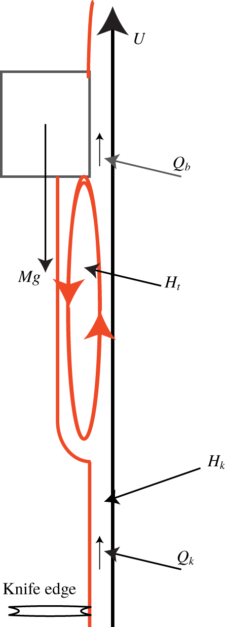
Now we suppose that a tongue, as in figure 8, is generated immediately beneath the block and has constant thickness  $H_{t}$. We also assume that the tongue terminates at a well-defined tip that is above the knife. The equations (3.15), (3.16) still hold and thus, in a steady flow, it is now the flux in the tongue that must be equated to the flux at the block so that
 $$\begin{eqnarray}Q_{b}=UH_{t}-\frac{\unicode[STIX]{x1D70C}gH_{t}^{3}}{3\unicode[STIX]{x1D707}};\end{eqnarray}$$
this gives two positive values for  $H_{t}$ when
 $Q_{b}$ is prescribed, as shown in figure 6. When we consider the corresponding velocity profile (3.15), we find that it is only when
 $H_{t}$ takes the larger of these values that the flow can recirculate, with fluid moving upwards near the belt but downwards near the film surface in accordance with the observation made at the end of § 2.
We also note that the response diagram for  $H_{t}(U)$, obtained using (3.13c) and (3.18), is
 $$\begin{eqnarray}\frac{\unicode[STIX]{x1D707}U^{2}LW}{2Mg}=UH_{t}-\frac{\unicode[STIX]{x1D70C}gH_{t}^{3}}{3\unicode[STIX]{x1D707}},\end{eqnarray}$$
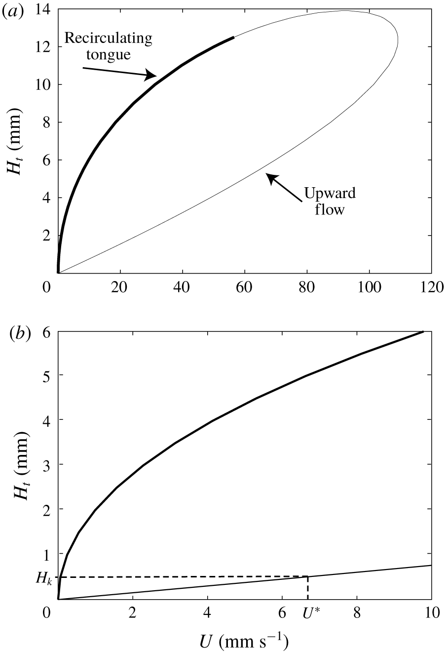
which limits the permissible values of  $U$ as shown in figure 9. The lower branch gives values of
 $H_{t}$ that are considerably smaller than those observed in § 2. We therefore conjecture that the upper branch indicated in bold in figure 9(a) is the one that is physically relevant in the tongue.
Schematic diagram illustrating the tongue which forms below the block.

(a) Plot of  $H_{t}$ versus
 $U$ evaluated using (3.19) with respective physical parameter values. (b) An expanded view over the parameter range which is relevant to the experiments. The location of
 $U^{\ast }$ for the film thickness
 $H_{k}=0.5~\text{mm}$ is indicated.

A comprehensive model for a recirculating tongue will require a more detailed analysis of the flow near  $x=0$ where the lubrication pressure is of
 $O(\unicode[STIX]{x1D707}U/\unicode[STIX]{x1D6FF}L)$. The velocity in such a region would be much smaller than
 $U$ away from the belt and thus could reduce the local capillary number,
 $U\unicode[STIX]{x1D707}/\unicode[STIX]{x1D70E}$ to be of
 $O(1)$, allowing a bulge to form in which surface tension and viscous terms are in balance. In such a region the pressure would have to be of
 $O(\unicode[STIX]{x1D70E}K)$, where
 $K$ is the curvature of the bulge, and
 $K$ would thus be of
 $O[(L\unicode[STIX]{x1D6FF})^{-1}Ca]$. However the local flow would lead to a free boundary problem for a fully two-dimensional Stokes flow which we will not attempt here. A similar local analysis would also be needed to reveal the flow details near the tongue tip.
This scenario changes dramatically when we allow the tongue tip to have a non-zero upward velocity  $V$ while still assuming the block to be stationary. Then
 $Q_{b}$ is no longer equal to
 $Q_{k}$ and conservation of mass at the tip requires that
 $$\begin{eqnarray}V=\frac{Q_{k}-Q_{b}}{H_{k}-H_{t}},\end{eqnarray}$$
which is negative if  $H_{t}>H_{k}$,
 $Q_{b}<Q_{k}$ and, as seen from figure 7, this occurs when
 $U<U^{\ast }$. Upward-moving tongues are theoretically possible if
 $U>U^{\ast }$ but experiments reveal that they always lead to block instability over short time scales.
The situation changes yet again when the tongue tip reaches the knife so that  $Q_{k}$ is no longer a control variable. The tongue thickness then remains constant throughout at the larger root of (3.18) and, as mentioned in § 2, this configuration is observed to be stable over time scales of hours.
We show a quantitative comparison between theoretical and experimental results for the propagation speed of the tongue as a function of the belt speed in figure 10. The relationship was calculated using (3.20) and the experimental estimates of the tongue speed were made by analysing sets of image sequences as described in the experimental section with reference to figure 4. The slopes of the time history plots were found to be linear although the block tended to tilt to the left or right at higher belt speeds and on occasions the motion was weakly time dependent. When  $(U^{\ast }-U)$ is small, the accord between the experimental results and the predictions of the two-dimensional was very satisfactory considering the three-dimensional effects at higher speeds in the experiment. However, it becomes more and more difficult to estimate
 $V$ as
 $(U^{\ast }-U)$ increases.
In summary, our simple two-dimensional model suggests that there is a range of values of  $U$ for which the block can remain stationary with
 $Q_{k}>Q_{b}$ as long as there is a tongue whose downward velocity is of the order of a few mm/min. On the other hand, for small values of
 $U^{\ast }-U$, the time scale for the tip motion is long compared with the transit time of the film through the device. We conjecture that the deviation between theory and observations as
 $U^{\ast }-U$ increases happens because a travelling wave is not attained before the tip reaches the knife edge.


4 Conclusions
At first sight, it is surprising that a rigid body can be levitated purely by viscous forces exerted by a vertically moving thin film. It is also surprising that long-term levitation can occur over a range of film velocities. We have shown that, for cuboidal bodies, classical lubrication theory leads to a situation in which the body is almost parallel to the belt that carries the film. The theory gives a simple formula for  $U^{\ast }$, the belt velocity needed for stationary levitation, but this result is only true to the lowest order in the ratio of the film thickness to the cuboid length. The fact that levitation can occur over a range of belt velocities is explained by the influence of the block on the film below it, which manifests itself as a downward-moving liquid tongue whose thickness is considerably greater than that of the incoming film.
It is interesting that we have been able to explain these phenomena using a quasi-steady two-dimensional lubrication model even though the lower boundary of the tongue is quite strongly curved in the third dimension. Finding the shape of the tongue tip is an important open question that may be able to be resolved by generalising the theory of Huppert (Reference Huppert1982). Another three-dimensional effect that we have not addressed is the rotation of the cuboid about an axis perpendicular to the belt which is frequently observed experimentally. More generally, it would be of interest to study levitating circular cylinders or spheres for which the extent of the lubrication region has to be determined as part of the problem. Also account would have to be taken of the rotation of the body and the associated film flow around its boundary. We remark that in the analogous problem of hot-glass rolling, large ‘bolsters’ of recirculating glass (Glynn & Storm Reference Glynn and Storm1965) are frequently observed in the vicinity of the initial point of contact between the glass and the roller.
Acknowledgements
The work of T.M. is supported by an Emeritus Fellowship (EM-2017-039/9) from the Leverhulme Trust. The experiments were performed in the Observatory in the Mathematical Institute and the authors are grateful to D. Vella for providing laboratory space. We are also grateful to L. Domino who helped measure the film thickness and to P. Howell and M. Dalwadi for helpful discussions.
Declaration of interests
The authors report no conflict of interest.
Appendix A
In order to find the lowest-order correction to (3.13) as  $\unicode[STIX]{x1D6FF}\rightarrow 0$ we rewrite the model in terms of the dimensionless variables
 $$\begin{eqnarray}\widetilde{p}=\frac{\unicode[STIX]{x1D6FF}^{2}Lp}{\unicode[STIX]{x1D707}U},\quad \widetilde{u}=\frac{u}{U},\quad \widetilde{x}=\frac{x}{L},\quad \widetilde{y}=\frac{y}{H_{k}},\quad \widetilde{h}=\frac{H}{H_{k}},\quad \widetilde{Q}=\frac{Q}{UH_{k}}.\end{eqnarray}$$
The model then involves  $\unicode[STIX]{x1D6FF}=H_{k}/L$ and, the other dimensionless parameters
 $$\begin{eqnarray}Re=UL/\unicode[STIX]{x1D708},\quad \unicode[STIX]{x1D6E4}=gL^{2}\unicode[STIX]{x1D6FF}^{2}/\unicode[STIX]{x1D708}U,\quad D/L\quad \text{and}\quad M_{\ast }=Mg\unicode[STIX]{x1D6FF}/\unicode[STIX]{x1D707}UW.\end{eqnarray}$$
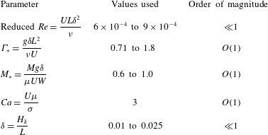
As shown in table 1, the Reynolds number only enters as  $Re\unicode[STIX]{x1D6FF}^{2}\ll 1$, while
 $D/L\sim M_{\ast }\sim O(1)$ and
 $\unicode[STIX]{x1D6E4}\sim \unicode[STIX]{x1D6FF}\sim O(10^{-1})$, so we also write
 $\unicode[STIX]{x1D6E4}_{\ast }=\unicode[STIX]{x1D6E4}/\unicode[STIX]{x1D6FF}$. When
 $\unicode[STIX]{x1D6FF}=0$ the lowest-order solution (3.13) is
 $$\begin{eqnarray}\widetilde{p}=0,\quad \widetilde{u}=1-M^{\ast }\widetilde{y},\quad \widetilde{h}=1/M_{\ast },\quad \widetilde{Q}=1/2M_{\ast }.\end{eqnarray}$$
To find the correction to  $O(\unicode[STIX]{x1D6FF})$, we write
 $$\begin{eqnarray}\widetilde{p}\sim \unicode[STIX]{x1D6FF}\widetilde{p_{1}},\quad \widetilde{h}=\frac{1}{M_{\ast }}(1+\unicode[STIX]{x1D6FF}\widetilde{h_{1}}+\unicode[STIX]{x1D6FF}\widetilde{m_{1}}\widetilde{x}),\quad \widetilde{Q}=\frac{1}{2M_{\ast }}(1+\unicode[STIX]{x1D6FF}\widetilde{Q_{1}}).\end{eqnarray}$$
We now exploit the fact that the dimensionless form of (3.9) is true to  $O(\unicode[STIX]{x1D6FF})$ to show that
 $$\begin{eqnarray}\widetilde{p_{1}}=(1-\widetilde{x})[\unicode[STIX]{x1D6E4}_{\ast }+6M_{\ast }^{2}(\widetilde{Q_{1}}-\widetilde{h_{1}})-3M_{\ast }^{2}\widetilde{m_{1}}(1+\widetilde{x})].\end{eqnarray}$$
Thus, since
 $$\begin{eqnarray}\int _{0}^{1}p\,\text{d}x=O(\unicode[STIX]{x1D6FF}^{2}),\end{eqnarray}$$
we find that
 $$\begin{eqnarray}\unicode[STIX]{x1D6E4}_{\ast }=4M_{\ast }^{2}\widetilde{m_{1}}-6M_{\ast }^{2}(\widetilde{Q_{1}}-\widetilde{h_{1}})\end{eqnarray}$$
and
 $$\begin{eqnarray}\widetilde{p_{1}}=M_{\ast }^{2}\widetilde{m_{1}}(1-\widetilde{x})(1-3\widetilde{x}).\end{eqnarray}$$
Similarly, the vertical force balance for the block gives that
 $$\begin{eqnarray}\widetilde{m_{1}}=\frac{6D}{M_{\ast }L}>0,\end{eqnarray}$$
which leads to the value of  $p(0)$ quoted at the end of § 3.1.
Non-dimensional parameters.

Finally, the torque balance gives that
 $$\begin{eqnarray}\widetilde{h_{1}}=-\frac{\unicode[STIX]{x1D6E4}_{\ast }}{2M_{\ast }^{2}}\quad \text{and}\quad \widetilde{Q_{1}}=\frac{4D}{M_{\ast }L}-\frac{2\unicode[STIX]{x1D6E4}_{\ast }}{3M_{\ast }^{2}}.\end{eqnarray}$$