1 Introduction
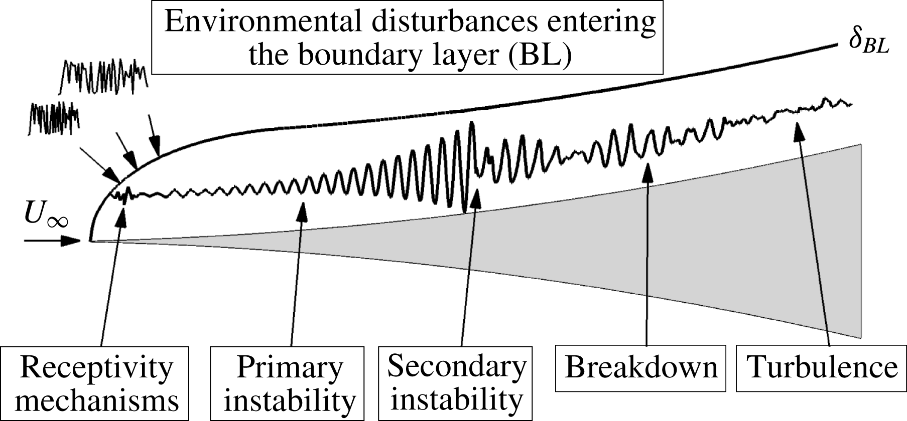
The various paths of hypersonic laminar–turbulent transition in boundary layers have been outlined by Morkovin (Reference Morkovin and Wells1969). For quiet tunnel conditions with low levels of free-stream turbulence, such as for the BAM6QT at Purdue University, the different stages of the transition process from the receptivity with respect to the natural disturbance environment all the way to turbulence are schematically shown in figure 1. Hader & Fasel (Reference Hader and Fasel2016, Reference Hader and Fasel2017) have carried out high-fidelity DNS for the BAM6QT conditions and flared cone geometry for a so-called ‘controlled’ breakdown. For these ‘controlled’ breakdown simulations the effect of free-stream turbulence and the receptivity process has been deliberately neglected. As shown by Hader & Fasel (Reference Hader and Fasel2016, Reference Hader and Fasel2017) the nonlinear breakdown in the Purdue flared cone experiments (Chynoweth et al. Reference Chynoweth, Ward, Henderson, Moraru, Greenwood, Abney and Schneider2014; Chynoweth Reference Chynoweth2015) is due to a so-called fundamental breakdown mechanism. It was sufficient for these simulations to initiate this breakdown by forcing a two-dimensional primary disturbance at a large (finite) amplitude and a pair of oblique (small amplitude) disturbance waves with the same frequency as the primary disturbance (fundamental breakdown) using a wall blowing/suction slot. Several numerical studies have shown that the fundamental breakdown appears to be a relevant breakdown mechanism for the BAM6QT conditions (Laible Reference Laible2011; Laible & Fasel Reference Laible and Fasel2011; Fasel, Sivasubramanian & Laible Reference Fasel, Sivasubramanian and Laible2015; Sivasubramanian & Fasel Reference Sivasubramanian and Fasel2016). Nevertheless, a desirable next step is to modify the disturbance forcing such that the restriction to ‘controlled’ breakdown in the numerical simulations is no longer necessary, thus allowing a disturbance input with a wide range of frequencies and wavenumbers as encountered in wind-tunnel experiments, and in particular also as encountered in conventional (‘noisy’) tunnels. This will allow the flow to naturally ‘select’ from the free-stream disturbances the dominant frequencies and wavenumbers, which can then amplify and interact nonlinearly, and thus ultimately lead to transition.
Overviews of the theoretical and experimental research regarding free-stream disturbances in high-speed boundary-layer transition are given, for example, in Pate (Reference Pate1980), Bushnell (Reference Bushnell1990), Schneider (Reference Schneider2001) and Wagner et al. (Reference Wagner, Schülein, Petervari, Hannemann, Ali, Cerminara and Sandham2018). In the following, for brevity, only a small subset of the references are addressed to motivate the proposed approach.
It is appropriate to start with the mode classification for free-stream disturbances according to Kovasznay (Reference Kovasznay1953), who distinguished between three types of disturbance modes: vorticity, entropy and sound. He states that pressure fluctuations in the free stream belong to the sound-wave modes. The detailed review by Pate (Reference Pate1980) on the effect of free-stream disturbances on boundary-layer transition suggests that in the hypersonic Mach number range, the radiated noise from the turbulent boundary layer at the nozzle walls is usually the dominant free-stream disturbance type affecting transition. This was also later supported by Bushnell (Reference Bushnell1990). Schneider (Reference Schneider2001) states that knowledge of the free-stream disturbance environment is essential to develop mechanism-based methods for transition prediction and argues that transition in tunnels nearly always originates from tunnel noise (Schneider Reference Schneider2004). Consequently, it appears to be necessary to take the tunnel noise into account for the DNS-based transition investigations to accurately reproduce the natural transition observed in the experiments. This would then require detailed characterization of the free-stream disturbance environment in the different experimental facilities used for hypersonic transition research. Parziale, Shepherd & Hornung (Reference Parziale, Shepherd and Hornung2014) quantified the free-stream perturbations in the Caltech T5 tunnel, and Duan, Choudhari & Zhang (Reference Duan, Choudhari and Zhang2016) carried out DNS to examine the pressure fluctuations generated by a turbulent boundary layer on the nozzle wall of the BAM6QT. In both cases the free-stream noise exhibited a broad frequency spectrum. Balakumar & Chou (Reference Balakumar and Chou2018) carried out DNS for a straight cone at Mach 10 to predict the transition onset location including the free-stream spectrum modelled according to detailed experimental measurements of the free-stream noise by Marineau et al. (Reference Marineau, Moraru, Lewis, Norris, Lafferty and Johnson2015). Balakumar & Chou (Reference Balakumar and Chou2018) found good agreement between experiments and numerical results when modelling the free-stream disturbance spectrum in the DNS.
Schematic of transition stages (Morkovin Reference Morkovin and Wells1969).

For the BAM6QT conditions and flared cone geometry, which is the subject of the present investigations, the free-stream disturbance spectrum is not yet known. Therefore, as a simple model, random forcing of pressure disturbances is applied at the inflow boundary of the computational domain to mimic tunnel noise in the experiments. The objective of the present investigation is to assess if and/or to what degree this simple free-stream disturbance model will be able to deliver realistic transition scenarios as observed in the experiments by Schneider and co-workers (Chynoweth et al. Reference Chynoweth, Ward, Henderson, Moraru, Greenwood, Abney and Schneider2014; Chynoweth Reference Chynoweth2015). In particular, it is of great interest to learn if this simple free-stream noise model leads to a nonlinear breakdown scenario that is consistent with the fundamental resonance mechanism that was found in our previous investigations to be the dominant mechanism (Hader & Fasel Reference Hader and Fasel2016, Reference Hader and Fasel2017) in the BAM6QT experiments.
2 Flow conditions and cone geometry
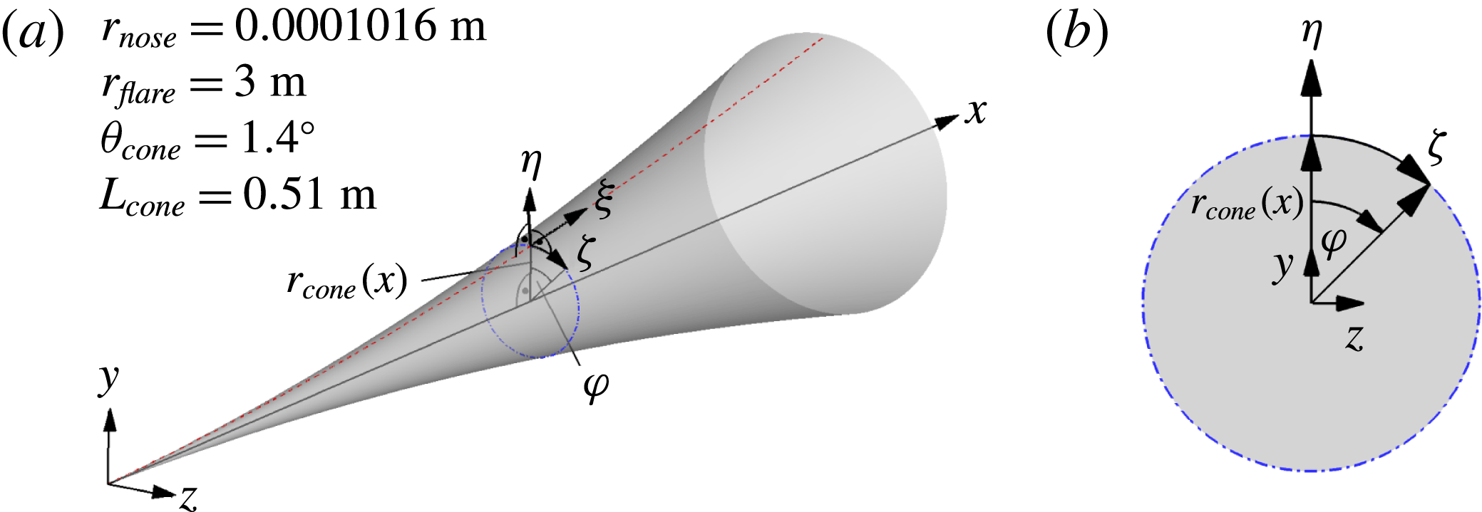
The breakdown simulation using the random forcing model was carried out for the Purdue flared cone geometry with a 4.5 inch base diameter that is used for the ongoing experiments in the BAM6QT (Chynoweth et al. Reference Chynoweth, Ward, Henderson, Moraru, Greenwood, Abney and Schneider2014; Chynoweth Reference Chynoweth2015). Schematics of the flared cone and the reference coordinate systems are provided in figure 2.
To facilitate a comparison to the ‘controlled’ (fundamental) breakdown simulations, the flow conditions are identical to those used by Hader & Fasel (Reference Hader and Fasel2016, Reference Hader and Fasel2017), where the free-stream Mach number is
 $M=6$
, a stagnation pressure of
 $p_{0}=140$
psi, and a stagnation temperature value of
 $T_{0}=420$
K, which results in the unit Reynolds number
 $Re_{1}=10.8\times 10^{6}~\text{m}^{-1}$
. The fluid is treated as a perfect gas with Prandtl number
 $Pr=0.71$
and ratio of specific heats
 $\unicode[STIX]{x1D6FE}=1.4$
. The viscosity is calculated using the standard Sutherland’s law without a low-temperature correction.
(a) Flared cone geometry and coordinate systems. (b) Flared cone cross section.

3 Random forcing approach
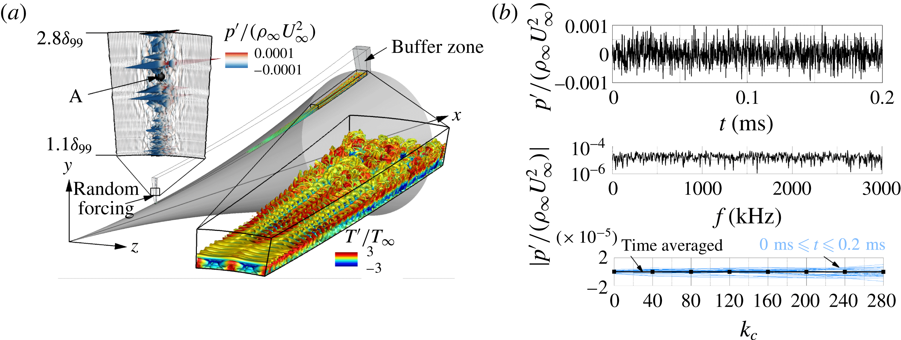
As a simple model of the free-stream wind-tunnel noise, random disturbances are introduced at the inflow boundary of the computational domain (figure 3
a). For the random forcing, the FORTRAN pseudo-random number generator is employed (compiler independent). To avoid repeating pseudo-random number sequences upon restart of the simulations, the system clock is used to initiate the pseudo-random sequence. The random perturbations (
 $p^{\prime }$
) are then applied at the pressure field to force acoustic sound-wave modes (Kovasznay Reference Kovasznay1953). The implementation allows for the random forcing to be applied at any user-specified locations of the computational domain
 $$\begin{eqnarray}\displaystyle p_{i,j,k,n}^{\prime }/(\unicode[STIX]{x1D70C}_{\infty }U_{\infty }^{2})=A_{noise}(2r-1),\quad \text{where}~r=\mathtt{random}\_\mathtt{number()}, & & \displaystyle\end{eqnarray}$$
the indices
 $i$
,
 $j$
and
 $k$
refer to the grid point indices in streamwise, wall-normal and azimuthal direction, respectively,
 $n$
represents the time step index,
 $r$
is the random number returned by the pseudo-random number generator, and
 $A_{noise}$
is the amplitude level of the random perturbations chosen by the user. For the presented results, the random forcing was applied at the symmetry line (
 $k=1$
) in the azimuthal direction, starting at the first grid point (which is at the wall) up to the last five grid points below the free-stream boundary (
 $1\leqslant j\leqslant 345$
) in the wall-normal direction, and from the sixth to the tenth grid point (
 $6\leqslant i\leqslant 10$
) in the streamwise direction. For the first five grid points in the streamwise direction and the five grid lines next to the free-stream boundary the disturbances are set to zero for convenience of implementation so as to not interfere with the Dirichlet boundary condition used for the laminar base flow at the inflow and free-stream boundaries. The random forcing was introduced only at
 $k=1$
in order to generate disturbances for a broad range of azimuthal wavenumbers. The computational setup is displayed in figure 3(a). The close-up view of the wall-normal plane in figure 3(a) shows the instantaneous random pressure disturbances introduced at the centreline of the inflow boundary. Upon closer inspection of figure 3(a), it can be seen that even though the random disturbances are only applied at the centreline, the perturbations quickly spread in the azimuthal direction. A close-up view of the flow field near the downstream end of the computational domain using isocontours of the Q-criterion (
 $Q=10\,000$
) coloured with the instantaneous temperature disturbance values in figure 3(a) indicates that the flow is transitioning in the downstream part of the domain due to the introduced random perturbations, as a breakdown to small structures can be observed. The time signal in figure 3(b) (top) extracted at point A (
 $i=10$
,
 $j=150$
,
 $k=1$
, see figure 3
a) in the free stream, which is approximately two boundary-layer thicknesses above the wall at the forcing location, shows that the introduced disturbances appear to be random. The corresponding frequency spectrum in figure 3(b) (middle) shows that this type of forcing introduces a wide range of frequencies as intended. The time-averaged azimuthal wavenumber spectrum in figure 3(b) (bottom), along with the instantaneous spectra calculated for various time instances
 $(0~\text{ms}\leqslant t\leqslant 0.2~\text{ms})$
after the initial transient has been convected out, indicate that the random forcing introduces a broad wavenumber spectrum without any noticeable bias.
(a) Computational setup for the DNS with random forcing; (b) time signal of the pressure disturbance at point A (top), the corresponding frequency spectrum (middle), the time-averaged azimuthal wavenumber spectrum (bottom, black solid line and square symbols), and the instantaneous wavenumber spectra for various time instances (bottom, light blue lines) after the initial transient has been convected out of the computational domain.

4 Results
The random forcing approach introduced above was applied to a high-resolution DNS to initiate laminar–turbulent transition. The computational domain with an extent of
 $0.15~\text{m}\leqslant x\leqslant 0.51~\text{m}$
,
 $0~\text{m}\leqslant \unicode[STIX]{x1D702}\leqslant 0.09~\text{m}~({\approx}100\unicode[STIX]{x1D6FF}_{99,outflow})$
and
 $0~\text{rad}\leqslant \unicode[STIX]{x1D711}\leqslant \unicode[STIX]{x03C0}/40~\text{rad}$
was resolved with
 $n_{x}=4750$
,
 $n_{\unicode[STIX]{x1D702}}=350$
and
 $n_{\unicode[STIX]{x1D711}}=129$
points in the streamwise, wall-normal and azimuthal directions, respectively. Here
 $\unicode[STIX]{x1D6FF}_{99}$
denotes the boundary layer thickness as the location where 99% of the edge velocity are reached. This setup is similar to the ones used for the ‘controlled’ breakdown simulations by Hader & Fasel (Reference Hader and Fasel2016, Reference Hader and Fasel2017). The details of the DNS code used here, along with its continuing development, have been described in Laible, Mayer & Fasel (Reference Laible, Mayer and Fasel2008, Reference Laible, Mayer and Fasel2009), Laible (Reference Laible2011), Laible & Fasel (Reference Laible and Fasel2011). For brevity only a short summary will be given. The numerical method is based on the three-dimensional Navier–Stokes equations, the continuity equation, and the energy equation for a compressible fluid in generalized conical coordinates. The so-called spatial model is applied, where all three spatial dimensions and time are discretized without any modelling assumptions. High-order accurate, non-compact, central finite differences are used for discretization of the wall-normal (fourth-order) and the streamwise direction (sixth-order). In the azimuthal direction, a pseudo-spectral discretization using fast Fourier transforms is employed. The inviscid fluxes are separated into an upwind flux and a downwind flux using van Leer’s splitting (van Leer Reference van Leer1982). Then, grid centred upwind biased differences (Zhong Reference Zhong1998) with ninth-order accuracy are applied to evaluate the derivatives for these fluxes. Special attention is given to the wall-next boundary stencils. Since high-order accurate boundary closures are typically unstable, the order of the stencil is successively reduced from ninth order to third order at the wall. The wall is assumed to be isothermal for the base flow and will remain so even in the presence of the disturbances. Consequently, the temperature disturbances at the wall vanish. The isothermal wall assumption with respect to the disturbances is justified because the wall temperature of the model remains nearly constant in the experiments due to the very short run times of the BAM6QT (see Ward Reference Ward2010; Chynoweth Reference Chynoweth2015). At the outflow boundary, a buffer is employed (see Meitz Reference Meitz1996) that effectively relaminarizes the flow. Here, the buffer is applied over 150 grid points from
 $4600\leqslant i\leqslant 4750$
. At the inflow and the free-stream boundary, five grid points are used to enforce the laminar base flow values obtained from a precursor calculation using a lower-order finite-volume code (for details see Gross & Fasel Reference Gross and Fasel2008). Periodicity and symmetry conditions are imposed at the azimuthal boundaries, allowing a reduction of the simulation domain by a factor of two. These boundary conditions were selected because they have been successfully employed in previous high-resolution DNS to study laminar–turbulent transition.
The random forcing described by (3.1) was applied at
 $6\leqslant i\leqslant 10$
,
 $1\leqslant j\leqslant 345$
and
 $k=1$
, as discussed above, with a noise level of
 $A_{noise}=10^{-2}$
. This noise level was selected based on the results from preliminary axisymmetric calculations, where the random forcing was applied at the same streamwise and wall-normal locations with varying values of
 $A_{noise}$
. The noise level was chosen such that the resulting saturation location of a primary wave was in the neighbourhood of that observed for the ‘controlled’ breakdown DNS to ensure that the nonlinear breakdown would occur in the computational domain. The choice to use
 $x=0.15$
m as the inflow boundary was based on the results of the linear stability regime (Hader & Fasel Reference Hader and Fasel2016), which showed that, at this location, the second mode is already amplified. This avoids the need to compute parts of the cone geometry where the disturbances are decaying, and therefore are not of interest for a nonlinear breakdown investigation. The domain height was designed such that the free-stream boundary is approximately 100 laminar boundary-layer thicknesses (calculated at the outflow) above the wall to minimize the effects of possible reflections from the free-stream boundary. The grid resolution was based on our previous experience with the controlled breakdown simulations (Hader & Fasel Reference Hader and Fasel2016, Reference Hader and Fasel2017). In these cases, the wall units (grid line spacing rescaled with the friction velocity) were
 $\unicode[STIX]{x0394}x_{max}^{+}\approx 6$
in the streamwise direction,
 $\unicode[STIX]{x0394}\unicode[STIX]{x1D702}_{max}^{+}\approx 1$
in the wall-normal direction, and
 $\unicode[STIX]{x0394}\unicode[STIX]{x1D701}_{max}^{+}\approx 2.3$
in the azimuthal direction, respectively. Consequently, the wall-normal grid line spacing is adequate to resolve the viscous sublayer and the streamwise and azimuthal wall units are comparable to the values reported in Mayer, Von Terzi & Fasel (Reference Mayer, Von Terzi and Fasel2011), who computed a complete breakdown all the way to turbulence for a flat plate at Mach 3.
Note that the extent of the computational domain in the azimuthal direction determines the smallest azimuthal wavenumber that is physically resolved in the simulation. The domain size of
 $\unicode[STIX]{x1D711}_{simulation}=\unicode[STIX]{x03C0}/40$
along with the symmetry conditions that are employed on the azimuthal boundaries limit the smallest azimuthal wavenumber that is contained in the simulation to
 $k_{c}=40$
. Consequently, only integer multiples of
 $k_{c}=40$
are resolved in the presented random forcing DNS.
The entire flow field was sampled for a duration of
 $T_{sampling}=2\times 10^{-4}$
s with a sampling frequency of
 $f_{sampling}=6$
MHz to accurately resolve frequencies up to 3 MHz with a frequency interval of
 $\unicode[STIX]{x0394}f=5$
kHz. With these sampling parameters, the most amplified second mode frequency band for the primary instability (the largest
 $N$
-factors were obtained for 300–350 kHz, see Hader & Fasel Reference Hader and Fasel2016) and the higher harmonics are adequately resolved. The flow was averaged (arithmetic average) for a duration of
 $T_{average}=2\times 10^{-3}$
s to obtain a value on the order of the tunnel run time at the BAM6QT facility. The wall pressure disturbance at the wall was sampled with
 $f_{sampling}=10$
MHz for a duration of
 $T_{sampling}=2\times 10^{-3}$
s allowing for a reasonable comparison to the experimental data that was recorded for
 $T_{sampling,experiment}=9.3\times 10^{-3}$
s at a rate of
 $f_{sampling,experiment}=5$
MHz (Chynoweth, B. 2017, private communication).
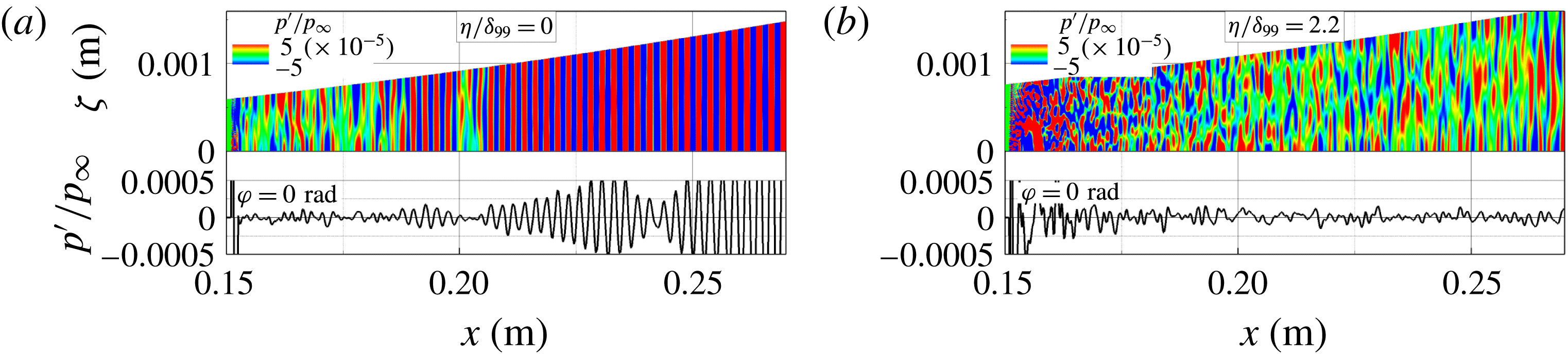
The normalized pressure disturbance contours are shown in figure 4 (top) along with the corresponding normalized pressure signals at the symmetry line (
 $\unicode[STIX]{x1D711}=0$
,
 $k=1$
) in figure 4 (bottom) at the same time instant (
 $t=1$
ms) when the initial transient has left the computational domain. The contours for the unrolled cone surface (
 $\unicode[STIX]{x1D701}$
, see figure 2
b) are shown in figure 4(a) (top). As can be observed, at the wall the random disturbances quickly contaminate the entire spanwise domain and then begin to form a coherent two-dimensional wave packet after a short downstream distance. The two-dimensional waves are the dominant second mode waves that are most unstable in high-speed boundary layers (Mack Reference Mack1969). This shows that the boundary layer naturally ‘selects’ the most unstable frequencies from the broadband spectrum introduced by the random forcing after a very short downstream distance. In contrast, the normalized pressure disturbance contours in the unrolled surface approximately two boundary-layer thicknesses away from the cone wall in figure 4(b) indicate the presence of random 3D patterns, which are equivalent to the acoustic noise in the free stream. The normalized pressure disturbance signals extracted at the symmetry line show that in the boundary layer, (figure 4
a, bottom) the randomly forced disturbances quickly form wave packets, whereas in the free-stream, (figure 4
b, bottom) random pressure fluctuations without a preferred wavelength are observed.
Pressure disturbance contours (top) and pressure disturbance signal at
 $\unicode[STIX]{x1D711}=0$
rad (bottom) at the same time instant (
 $t=1$
ms). (a) For the unrolled cone surface and (b) in an unrolled surface at a distance
 $\unicode[STIX]{x1D702}/\unicode[STIX]{x1D6FF}_{99}=2.2$
from the cone wall.

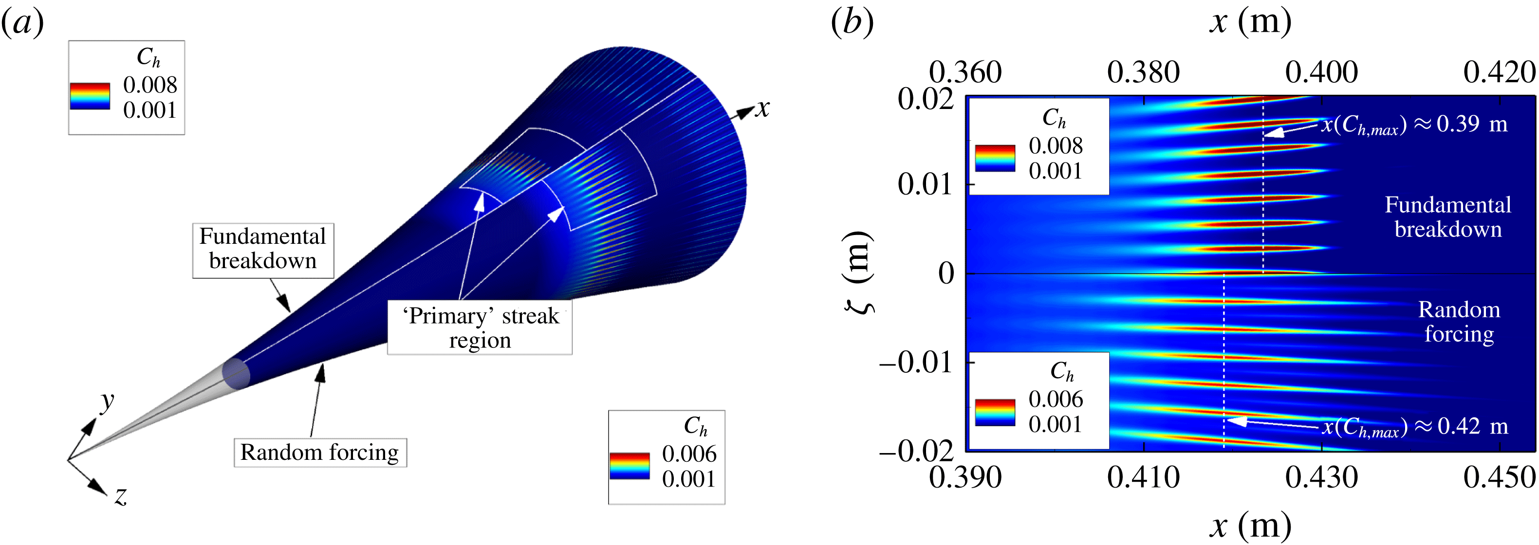
A comparison of the time-averaged Stanton number contours on the surface of the cone between the results from the DNS of the ‘controlled’ fundamental breakdown (Hader & Fasel Reference Hader and Fasel2016) and the DNS results with random forcing is provided in figure 5(a). For the ‘controlled’ fundamental breakdown a large-amplitude two-dimensional primary wave (
 $f=300$
kHz) was forced together with a pair of small-amplitude three-dimensional secondary waves at the same frequency using wall-normal velocity disturbances through a wall blowing/suction slot. For the secondary wave, the azimuthal wavenumber that led to the largest secondary growth rate after resonance onset was chosen (
 $k_{c}=80$
). Compared to the ‘controlled’ fundamental breakdown, the random forcing approach does not favour any particular disturbance waves, both with respect to frequency and azimuthal wavenumbers (that are resolved in the computational domain), but rather introduces a wide range of frequencies and azimuthal wavenumbers at the inflow boundary of the computational domain (figure 3
b). As can be observed in figure 5 for both the ‘controlled’ and random forcing simulations, ‘primary’ streaks appear for a limited downstream extent until ‘secondary’ streaks appear farther downstream where the flow has already progressed far into the highly nonlinear breakdown regime (figure 5
a). Although the ‘primary’ streaks and the ‘secondary’ streaks do not appear at exactly the same downstream locations for the two cases, it is remarkable that the random forcing approach leads to a pattern of streamwise streaks as observed in the ‘controlled’ breakdown simulation and in the BAM6QT experiments. A close-up of the ‘primary’ streak region (unrolled in azimuthal direction) is provided in figure 5(b). In the top half, the ‘primary’ streak region obtained for the ‘controlled’ fundamental breakdown is shown and compared to the ‘primary’ streaks observed for the random forcing breakdown on the bottom half. As shown by Laible (Reference Laible2011), and Laible & Fasel (Reference Laible and Fasel2011), all other conditions being identical, reducing the initial primary disturbance amplitude slightly would shift the streak onset farther downstream. As a result, both the onset location and the downstream extent of the streaks observed in the ‘controlled’ breakdown simulations depend on the initial amplitudes of the primary and secondary disturbance waves.
(a) Time-averaged Stanton number contours on the surface of the cone (left: ‘controlled’ fundamental breakdown; right: random forcing breakdown) and (b) a close-up of the ‘primary streak’ region (unrolled in azimuthal direction) for the ‘controlled’ fundamental breakdown (top) and the random forcing breakdown (bottom).

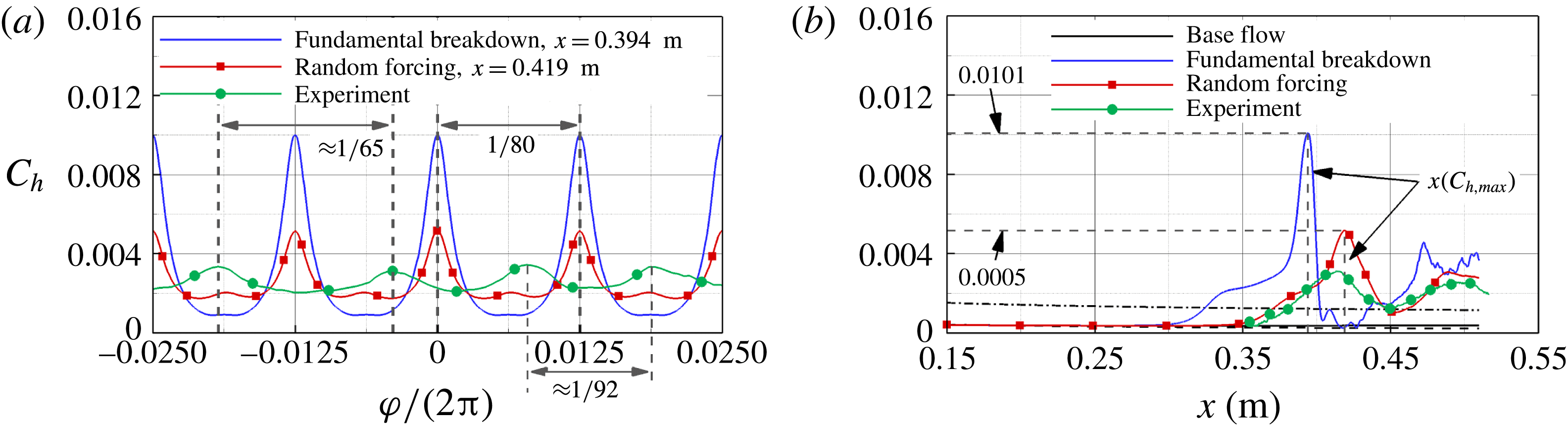
The azimuthal spacing of the ‘primary’ streaks obtained with the ‘controlled’ breakdown DNS, the random forcing DNS and the experiments at BAM6QT (
 $p_{0}=131.9$
psi,
 $T_{0}=432.6$
K,
 $Re_{1}=9.7\times 10^{6}~\text{m}^{-1}$
, Chynoweth, B. 2017, private communication) is compared in figure 6(a). For the DNS results a total of 80 ‘primary’ streaks around the circumference of the cone can be observed. The distance in the azimuthal direction between the ‘primary’ streaks obtained in the experiments is not constant but is in the same range as for the DNS. The cause for the misalignment of the streaks between experimental and numerical results is not yet known and will be subject to future investigations. Whereas for the ‘controlled’ fundamental breakdown case the secondary wave was forced with an azimuthal wavenumber of
 $k_{c}=80$
(Hader & Fasel Reference Hader and Fasel2016, Reference Hader and Fasel2017), no particular azimuthal wavenumber was favoured in the random forcing breakdown case (except that due to the limited azimuthal domain extent only azimuthal wavenumbers which are an integer multiple of
 $k_{c}=40$
are resolved in the simulation). This indicates that the assumption made for the ‘controlled’ breakdown simulations, namely that in a ‘natural’ breakdown scenario the secondary wave with the largest integrated growth rate (
 $N$
-factor) after the secondary resonance onset is the 3D wave that will most likely prevail and dominate the nonlinear regime and thus the ‘primary’ streak development, is valid (provided of course that the fundamental resonance scenario is indeed the route to transition for the given flow conditions and geometry of the Purdue experiments). Therefore, the results of the random forcing DNS are providing further (almost conclusive) evidence that the observed streaks in the Purdue experiment are indeed due to a fundamental resonance. Further support for this can be obtained by comparing the downstream development of the time-averaged Stanton number between the ‘controlled’ fundamental breakdown, the random forcing case and the experiments (Chynoweth, B. 2017, private communication) as provided in figure 6(b). The Stanton number development for the base flow as well as for the laminar and turbulent estimate for a straight cone (White Reference White2006) are provided for reference. For all cases, after an initial departure from the laminar curve, the Stanton number increases slowly at first before rising rapidly when the ‘primary’ streaks begin to form, resulting in a massive overshoot far beyond the turbulent estimates. When the ‘primary’ streaks disappear, the time-averaged Stanton number drops almost back to the laminar base flow value. When the ‘secondary’ streaks appear, the time-averaged Stanton number rises again; however, the peak values are lower than for the ‘primary’ streaks. The Stanton number development in the downstream direction of the random forcing DNS and the experimental results show remarkable agreement.
Comparison of the time-averaged Stanton number for the fundamental breakdown DNS (Hader & Fasel Reference Hader and Fasel2016), the random forcing DNS (for
 $p_{0}=140$
psi,
 $T_{0}=420$
K,
 $Re_{1}=10.8\times 10^{6}~\text{m}^{-1}$
) and the experimental results (for
 $p_{0}=131.9$
psi,
 $T_{0}=432.6$
K,
 $Re_{1}=9.7\times 10^{6}~\text{m}^{-1}$
, courtesy of Chynoweth, B. 2017, private communication) in (a) the azimuthal direction and (b) the downstream direction at
 $\unicode[STIX]{x1D711}=0$
rad.

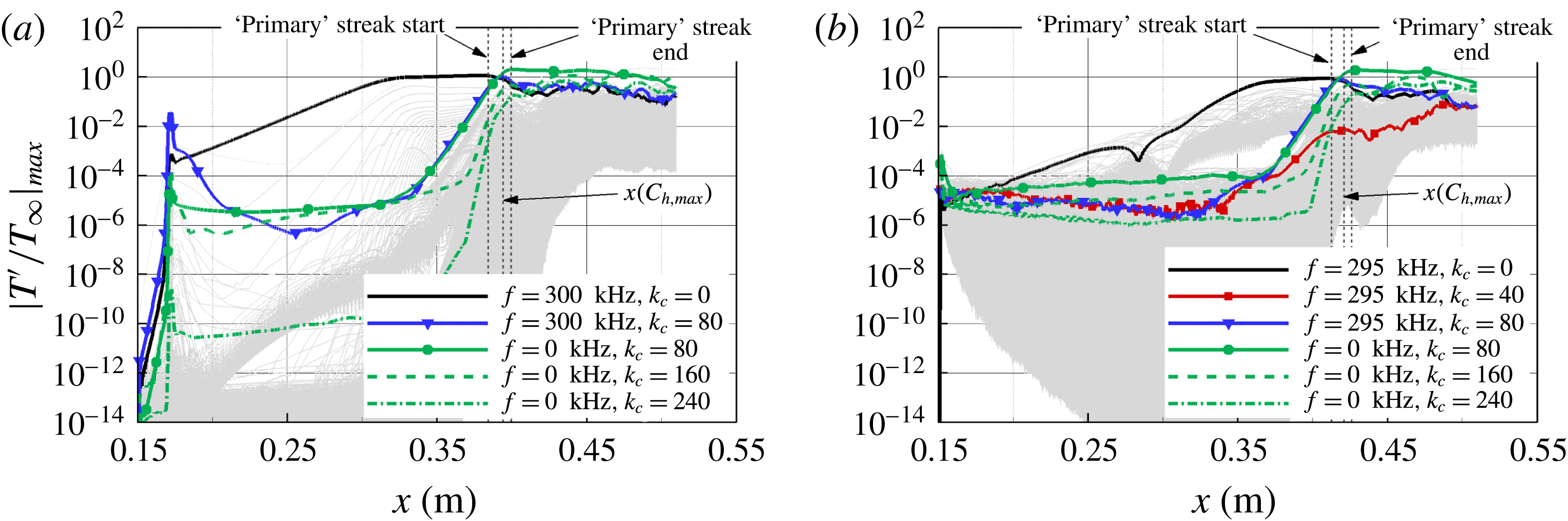
The downstream development of the maximum temperature amplitudes of various disturbance components for the ‘controlled’ fundamental resonance case is compared to the random forcing case in figure 7. With the random forcing (figure 7
b), all two- and three-dimensional disturbance modes (resolved in the computational domain) at a wide range of frequencies (see figure 7
b) are introduced at approximately the same amplitude level, whereas for the fundamental breakdown (figure 7
a) only the primary wave and the secondary wave are forced, and are introduced at much larger amplitudes compared to the numerical background noise caused by the discretization error. Based on a low-amplitude axisymmetric pulse simulation (Hader & Fasel Reference Hader and Fasel2016), the primary wave frequency to be used for the ‘controlled’ fundamental breakdown simulation was
 $f=300$
kHz, as for this frequency the largest
 $N$
-factor was obtained. For the random forcing case, no single frequency is favoured by the broadband forcing, and the individual modes are allowed to develop naturally in the downstream direction. In this scenario, the two-dimensional second mode with a frequency of
 $f=295$
kHz appears to dominate over the other frequency modes, which is in remarkable agreement with the
 $f=300$
kHz of the primary wave used for the ‘controlled’ fundamental breakdown case. Based on our investigations of the primary instability (see Hader & Fasel Reference Hader and Fasel2016) the branch I neutral point for both frequencies is
 $x_{0,I}\approx 0.085$
m and the spatial growth rates vary in the range
 $60~\text{m}^{-1}\leqslant -\unicode[STIX]{x1D6FC}_{i}\leqslant 70~\text{m}^{-1}$
. Compared to the ‘controlled’ fundamental breakdown in figure 7(a), for the random forcing case (figure 7
b) the three-dimensional disturbance waves with the various spanwise wavenumbers are all ‘starting’ at approximately the same amplitude levels. None of the 3D modes are initially amplified until they experience strong growth once the two-dimensional waves start to saturate close to
 $x\approx 0.35$
m. Consistent with the fundamental resonance study by Hader & Fasel (Reference Hader and Fasel2016), the disturbance wave with an azimuthal wavenumber of
 $k_{c}=80$
grows most rapidly, and nonlinearly generates the steady longitudinal mode with the same azimuthal wavenumber together with the two-dimensional wave of the same frequency:
 $(f=295~\text{kHz},k_{c}=0)\pm (f=295~\text{kHz},k_{c}=80)\rightarrow (f=0~\text{kHz},k_{c}=80)$
. The (
 $f=0$
kHz,
 $k_{c}=80$
) mode is the dominant mode when the ‘primary’ streaks appear, and reaches its maximum when the time-averaged Stanton number becomes maximal. The azimuthal wavenumber of this dominant longitudinal mode determines the ‘primary’ azimuthal streak count. The ‘primary’ streaks disappear because the streamwise vortices that are responsible for their formation are lifted away from the wall. Further downstream these vortices are pushed back towards the wall, leading to the ‘secondary’ streaks (see Hader & Fasel Reference Hader and Fasel2016). At this point, the ‘controlled’ as well as the random forcing DNS results show that higher harmonics (
 $k_{c}=160$
,
 $k_{c}=240$
) of the dominant steady streamwise mode (
 $k_{c}=80$
) have reached large amplitudes (figure 7), causing an increased streak count, as observed by Hader & Fasel (Reference Hader and Fasel2016) for the ‘controlled’ breakdown simulation.
Downstream development of the maximum temperature amplitude for various disturbance components: (a) ‘controlled’ fundamental breakdown, (b) random forcing DNS.

The amplitude development comparison in figure 7 clearly indicates that even for the random forcing, which does not favour any particular frequencies or azimuthal wavenumbers (in contrast to the ‘controlled’ forcing case), the fundamental resonance is indeed the relevant mechanism for the investigated geometry and flow conditions.
Comparison of experimental measurements at the BAM6QT (
 $p_{0}=131.9$
psi,
 $Re_{1}=9.7\times 10^{6}~\text{m}^{-1}$
) to DNS results (
 $p_{0}=140.0$
psi,
 $Re_{1}=10.8\times 10^{6}~\text{m}^{-1}$
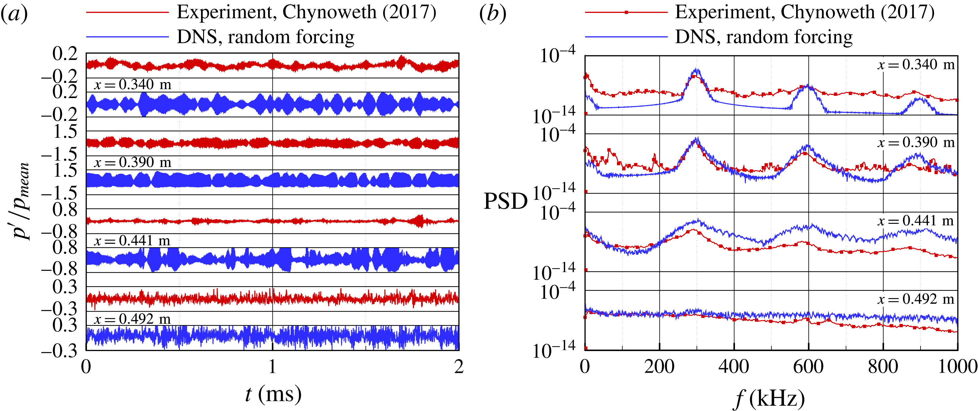
): (a) normalized wall pressure disturbance over time and (b) corresponding PSD spectra.

A comparison of simulation data with measurements from the BAM6QT is provided in figure 8. The experimental data are for
 $p_{0}=131.9$
psi,
 $Re_{1}=9.7\times 10^{6}~\text{m}^{-1}$
and were provided by (Chynoweth, B. 2017, private communication). Although the provided experimental data are for conditions slightly different than those used in the simulation (
 $p_{0}=140$
psi,
 $Re_{1}=10.8\times 10^{6}~\text{m}^{-1}$
), a direct comparison nevertheless provides valuable insights. The experimental time signals of the normalized pressure disturbance at the wall at the various pressure sensor locations (figure 8
a) show good qualitative agreement with results from the random forcing DNS. The experiment and simulation time signals in figure 8(a) show ‘wave packet like intermittency’, with sequences of wave packets that are ‘chasing’ each other. Despite the slightly different flow conditions between experiment and DNS, the main trends are consistent with each other. The amplitudes of the normalized pressure disturbances obtained with the random forcing DNS are of the same order of magnitude as the experimental measurements (figure 8
a). The amplitude of the experimental signal at
 $x=0.441$
m has dropped significantly compared to the amplitude at
 $x=0.390$
m due to energy being distributed over a wider range of frequencies and azimuthal wavenumbers, whereas the amplitude of the simulation data shows a less drastic drop when comparing these two locations. This is most likely caused by the fact that the experiment may already have progressed further into the breakdown regime compared to the simulation at this particular downstream location. At
 $x=0.492$
m the experimental time signal as well as the simulation data show random fluctuations, and the wave packet character of the time signals as seen at the upstream locations has disappeared. The corresponding PSD spectra for both experimental and simulation data have been calculated using the post-processing script provided by (Chynoweth, B. 2017, private communication). The comparison in figure 8(b) shows remarkable agreement between experiments and the random forcing DNS. The dominant amplified frequency bands from the experimental data are well captured in the simulations. The PSD amplitudes are in reasonable agreement (computed amplitudes are two to three times larger compared to the measured amplitudes) at
 $x=0.390$
m and
 $x=0.492$
m, considering the differences in flow conditions and the limitations of the simulation regarding the azimuthal domain width, which only allows for azimuthal wavenumbers of
 $k_{c}=40$
and its higher harmonics compared to the experiments, where no such limitations are present. The differences at the other locations can be attributed to the difference in flow conditions as well as the fact that the ‘primary’ streaks and the ‘secondary’ streaks appear further downstream in the DNS compared to the experimental data. As discussed already in connection with the results shown in figure 5, the streak onset can be moved in the upstream or downstream directions by increasing or decreasing, respectively, the initial forcing amplitude.
5 Conclusions
The objective of this research is to contribute towards the understanding of ‘natural’ boundary-layer transition in high-speed wind-tunnel experiments where the transition is caused by the free-stream disturbances of the experimental facility (in contrast to the so-called ‘controlled’ transition). Towards this end, DNS are employed to investigate the effects of free-stream (broad frequency band) pressure disturbances on the nonlinear stages of hypersonic boundary-layer transition.
A simple random forcing approach is proposed and investigated, by which random pressure disturbances were introduced at the inflow boundary of the computational domain that are generated by a random number generator. This approach reflects an attempt to provide a simple model to account for the free-stream (acoustic) disturbance field in wind-tunnel experiments (both ‘quiet’ and conventional) when detailed information regarding the free-stream (acoustic) disturbance environment is not available. The usefulness and validity of the random forcing approach for high-speed transition investigations using DNS was demonstrated by a ‘natural’ transition simulation of the transition experiments for a flared cone at Mach 6 conducted in the BAM6QT at Purdue University. The simulation results using the random forcing approach for a flared cone and the BAM6QT flow conditions exhibited essentially the same nonlinear breakdown mechanisms as observed in our previous ‘controlled’ DNS of fundamental breakdown. In particular, the random forcing simulations yielded the same pattern of ‘primary’ streamwise ‘hot’ streaks, which appears for a short downstream extent, then disappears, followed by a pattern of ‘secondary’ streaks at the onset of the final breakdown to turbulence. The same patterns of hot streaks have also been observed in the BAM6QT experiments at Purdue University.
In addition to the hot streak patterns, the simulations using the random forcing model led to approximately the same dominant frequencies, which are determined by the linear stability characteristics of the second mode waves, and to the spanwise wavenumbers for the primary and secondary waves in the nonlinear transition stages as observed in the experiments. The azimuthal wavenumber spectrum was, however, limited to integer multiples of
 $k_{c}=40$
due to the restriction of the computational domain extent in azimuthal direction. For future investigations the domain size will be increased to investigate if other azimuthal wavenumbers that were not resolved in the presented results could play a prominent role in the laminar–turbulent transition process. In summary, the investigation presented provides strong support for the use of the proposed random forcing model for DNS of high-speed boundary-layer transition when detailed information regarding the free-stream disturbance field in wind-tunnel tests and/or free flight is not available. Furthermore, these simulation results provide additional and almost conclusive confirmation that fundamental breakdown is indeed the relevant nonlinear mechanism in the Purdue flared cone experiments, and thus confirming also that ‘controlled’ fundamental breakdown simulations can capture the relevant nonlinear mechanisms of natural transition when carefully planned and executed.
Acknowledgements
This work was supported by AFOSR Grant FA9550-15-1-0265, with Dr I. Leyva serving as programme manager. Computer time was provided by the US Army Engineering Research and Development Center (ERDC) under the Department of Defense (DOD) High Performance Computing Modernization Program (HPCMP). The views and conclusions contained herein are those of the authors and should not be interpreted as necessarily representing the official policies or endorsements, either expressed or implied, of the Air Force Office of Scientific Research or the US Government. The authors would like to express their gratitude to Brandon Chynoweth and Professor S. Schneider (Purdue University) for their support by providing measurement data and post-processing scripts and the many fruitful discussions that helped to improve our simulations.