



1. Introduction
The Coulomb-driven instability of dielectric liquids subjected to strong unipolar injection of ions is a classical problem in electrohydrodynamics (EHD). When the working fluid is a viscoelastic polymer solution, the elasticity of the fluid markedly changes the instability characteristics. Su et al. (Reference Su, Zhang, Luo and Yi2020) were the first to numerically solve the fully coupled governing equations for an Oldroyd-B dielectric liquid under unipolar injection, revealing that the primary instability may set in through either a supercritical or a Hopf bifurcation, in contrast to the subcritical bifurcation for the Newtonian case. They further found that the stability threshold remains unaffected by elasticity at sufficiently small Weissenberg number, but decreases once the primary instability becomes a Hopf bifurcation. Subsequently, Zhang et al. (Reference Zhang, Li, Su, Wu and Yi2022) reported a supercritical bifurcation in a coaxial cylinder geometry. These advances, however, all rest on direct numerical simulation. Yao et al. (Reference Yao, Zhang, Wu, Luo and Yi2025b
) numerically determined the neutral stability boundary for quiescent Oldroyd-B electroconvection and distinguished stationary from oscillatory onset over the comparatively small range of
 $\textit{Wi}$
considered in their study; they also examined convective and absolute instabilities in the presence of a Poiseuille base flow. Their study did not, however, derive a reduced analytical dispersion relation for the neutral frequency and threshold or address their asymptotic behaviour in the strongly elastic regime up to
 $\textit{Wi}=10^{3}$
. An analytical description of oscillatory electroconvection in this regime therefore remains lacking. Experimentally, Wu et al. (Reference Wu, Yang, Sun, Huang and Yang2026) used particle image velocimetry to compare needle–plate EHD plumes in newly formulated polyisobutylene (PIB)-based viscoelastic dielectric liquids with those in the Newtonian base liquid, and found that increasing elasticity causes the plume velocity to become fully developed closer to the needle tip. An analytical theory for the onset of oscillatory instability in viscoelastic EHD flows, and in particular the scaling behaviour in the strongly elastic regime, remains largely lacking. More broadly, this quiescent configuration provides a clear model of relaxation-controlled instability in complex fluids, in which competition between stress relaxation and destabilising transport can induce overstability and reveal its strongly elastic limit.
Within the related field of electrokinetics, Borthakur & Ghosh (Reference Borthakur and Ghosh2023) analysed the electrophoretic motion of non-uniformly charged particles in an Oldroyd-B fluid under the thin-electrical-double-layer and weak-viscoelasticity limits. Roy & Dhar (Reference Roy and Dhar2024) examined oscillatory electro-magneto-imbibition of a Phan–Thien–Tanner viscoelastic electrolyte in non-uniform microcapillaries. Li et al. (Reference Li, Archer and Koch2019) showed that polymer elasticity promotes an earlier transition to unsteady electroconvection and reduces the overlimiting current in a liquid electrolyte. Kouni et al. (Reference Kouni, Moschopoulos, Dimakopoulos and Tsamopoulos2023) reported that the sedimentation velocity of a charged sphere in a viscoelastic electrolyte approaches an asymptote as further polymer stretching and changes in the electric force become limited. These results demonstrate that high-
 $\textit{Wi}$
saturation can occur in different electrically coupled viscoelastic flows.
Such elasticity-induced overstability has been thoroughly studied in Rayleigh–Bénard thermal convection. Vest & Arpaci (Reference Vest and Arpaci1969) were the first to show that a viscoelastic fluid layer heated from below can become overstable, with oscillatory convection setting in before steady convection. Khayat (Reference Khayat1994), using a Lorenz type truncated system, demonstrated that the threshold for steady convection is independent of elasticity below a critical Deborah number, whereas above it, the onset switches to an overstable mode. Martínez-Mardones et al. (Reference Martínez-Mardones, Tiemann, Walgraef and Zeller1996) derived the corresponding analytical thresholds and amplitude (oscillation) equations. More recently, Yao et al. (Reference Yao, Lu, Zhang, Luo and Yi2025a ) studied Rayleigh–Bénard convection of Oldroyd-B fluids both in the quiescent case and under a Poiseuille base flow. Such thermal convection analyses, however, largely rely on low order truncations, can determine the onset frequency only numerically and pertain to supercritical bifurcations. Electroconvection, by contrast, is Coulomb-driven: its base state is set by the charge transport equation rather than by thermal diffusion, its bifurcation is subcritical and the migration of free charge introduces physics different from thermal convection.
In this paper, we show that the quiescent base state of electroconvection renders this viscoelastic instability problem closed and analytically tractable. A single-mode Galerkin projection based on the Newtonian critical eigenfunction is then used to construct a reduced analytical model for the oscillatory neutral state. The resulting dispersion relation provides a closed-form prediction for the neutral frequency and yields asymptotic scaling laws for the threshold and frequency in the strongly elastic regime. We further extend the full spectral stability analysis to
 $\textit{Wi} \sim 10^{3}$
, and identify a three-stage variation of the critical electric Rayleigh number with
 $\textit{Wi}$
. Once its geometric coefficient is determined from one reference case, the reduced model agrees with the spectral results to within
 $0.3\,\%$
over the parameter range examined.
2. Problem formulation and equations
2.1. Governing equations
We consider a layer of incompressible viscoelastic Oldroyd-B dielectric liquid confined between two infinite parallel electrodes separated by a gap
 $H$
, with unipolar charge injection from one electrode. The magnetic effect is neglected due to the weak electric current. We take the electrode spacing
 $H$
as the characteristic length scale, the injecting-electrode voltage
 $V_0$
as the electric-potential scale and the corresponding ionic drift velocity
 $K_iV_0/H$
as the velocity scale, where
 $K_i$
is the dimensional ionic mobility. The resulting ionic-drift time scale is
 $H^2/(K_iV_0)$
. The electric field, free-charge density and pressure are scaled by
 $V_0/H$
,
 $\epsilon V_0/H^2$
and
 $\rho (K_iV_0/H)^2$
, respectively, where
 $\epsilon$
and
 $\rho$
are the permittivity and density of the liquid. The polymer stress is scaled by
 $\eta _pK_iV_0/H^2$
, where
 $\eta _p$
is the polymer contribution to the total zero-shear viscosity
 $\eta _0=\eta _s+\eta _p$
. Accordingly, the dimensionless electric potential and electric field satisfy
 $\boldsymbol{E}=-\boldsymbol{\nabla }\phi$
. Under the electroquasistatic approximation for an incompressible dielectric liquid with uniform permittivity, the electrical body force reduces to the Coulomb force
 $q\boldsymbol{E}$
, with magnetic effects neglected because of the weak electric current. The dimensionless governing equations follow the physical model of Su et al. (Reference Su, Zhang, Luo and Yi2020):
 \begin{gather} \boldsymbol{\nabla }\boldsymbol{\cdot }\boldsymbol{u} = 0 ,\end{gather}
 \begin{gather} \frac {\partial \boldsymbol{u}}{\partial t} + \boldsymbol{u} \boldsymbol{\cdot }\boldsymbol{\nabla }\boldsymbol{u} = -\boldsymbol{\nabla }\!p + \frac {M^{2}}{T}\big (\beta {\nabla} ^{2} \boldsymbol{u} + (1-\beta )\boldsymbol{\nabla }\boldsymbol{\cdot }\boldsymbol{\tau }_{\!p}\big ) + M^{2} q \boldsymbol{E}, \end{gather}
 \begin{gather} \textit{Wi} \, \overset {\triangledown }{\boldsymbol{\tau }}_{\boldsymbol{p}} + \boldsymbol{\tau }_{\boldsymbol{p}} = \boldsymbol{\nabla }\boldsymbol{u} + \boldsymbol{\nabla }\boldsymbol{u}^{T}, \end{gather}
 \begin{gather} \boldsymbol{\nabla} ^{2} \phi = -q, \end{gather}
 \begin{gather} \frac {\partial q}{\partial t} + \boldsymbol{\nabla }\boldsymbol{\cdot }(q\boldsymbol{u}) + \boldsymbol{\nabla }\boldsymbol{\cdot }(q\boldsymbol{E}) - \frac {1}{\textit{Fe}}{\nabla} ^{2} q = 0. \end{gather}
At the injecting electrode, the boundary conditions are
 $\boldsymbol{u}=\boldsymbol{0}$
,
 $\phi =1$
and
 $q=C$
, whereas at the collecting electrode, they are
 $\boldsymbol{u}=\boldsymbol{0}$
,
 $\phi =0$
and
 $\boldsymbol{n}\boldsymbol{\cdot }\boldsymbol{\nabla }q=0$
, where
 $\boldsymbol{n}$
is the unit normal to the electrode. The governing dimensionless parameters are
 \begin{align} T=\frac {\epsilon V_0}{\eta _0K_i},\quad M=\frac {1}{K_i}\sqrt {\frac {\epsilon }{\rho }},\quad C=\frac {q_{\textit{inj}}^*H^2}{\epsilon V_0}, \\[-12pt]\nonumber \end{align}
 \begin{align} \textit{Fe}=\frac {K_iV_0}{D_i},\quad \textit{Wi}=\frac {\lambda K_iV_0}{H^2},\quad \beta =\frac {\eta _s}{\eta _0}, \end{align}
where
 $q_{\textit{inj}}^*$
is the dimensional charge density prescribed at the injecting electrode,
 $D_i$
is the charge diffusivity and
 $\lambda$
is the polymer relaxation time. Here,
 $T$
is the electric Rayleigh number,
 $M$
is the mobility ratio,
 $C$
is the injection strength,
 $\textit{Fe}$
is the electric Péclet number,
 $\textit{Wi}$
is the Weissenberg number and
 $\beta$
is the solvent-to-total viscosity ratio. The Newtonian response is recovered either at
 $\textit{Wi}=0$
, when the polymer stress relaxes instantaneously, or at
 $\beta =1$
, when the polymeric viscosity contribution vanishes.
The flow is in a quiescent base state,
 $\bar {u} = 0$
,
 $\overline {\tau }_{p} = 0$
. The strong-injection and weak-diffusion approximations are invoked only to obtain the analytical base state in (2.2). The full charge-transport equation and the subsequent linear stability problem retain charge diffusion through the term
 $\textit{Fe}^{-1}\boldsymbol{\nabla} ^2 q$
in (2.1e
). The base-state charge density and electric field admit a closed-form analytical solution of the one-dimensional steady charge-transport problem in the strong-injection and weak-diffusion limit,
 $C\gg 1$
and
 $\textit{Fe}\gg 1$
(equivalently,
 $\textit{Fe}^{-1}\to 0$
) (Atten & Moreau Reference Atten and Moreau1972), the field strength coefficient
 $E_{s}$
is evaluated for different injection strengths
 $C$
as
 \begin{equation} \overline {q(y)} = \frac {C}{\sqrt {1+2Cd/E_{s}}}, \quad \bar E(y) = E_{s}\sqrt {1+2Cd/E_{s}}, \quad \text{where } \quad d = \frac {y+1}{2} \in [0,1], \end{equation}
 \begin{equation} \frac {2E_{s}^{2}}{3C}\left [\left (1+\frac {2C}{E_{s}}\right )^{\frac {3}{2}} - 1\right ] = 2, \end{equation}
where
 $y\in [-1,1]$
is the wall-normal coordinate and
 $d$
is the corresponding affine coordinate, with
 $d=0$
at the injecting electrode and
 $d=1$
at the collecting electrode. Here,
 $\bar {q}(y)$
and
 $\bar {E}(y)$
denote the base-state charge density and wall-normal electric-field strength, respectively. The
 $\bar {q}(-1)=C$
, while
 $E_s\equiv \bar {E}(-1)$
is the electric-field strength at the injecting electrode.
2.2. Linearised and normalised equations
Perturbations are taken in the normal-mode form
 $F'(x,y,t) = \widehat {F}(y)\exp (\mathrm{i}kx + \sigma t)$
, where
 $\sigma = \sigma _{r} + \mathrm{i}\sigma _{i}$
is the complex growth rate (
 $\sigma _{r} \gt 0$
corresponds to instability). After linearising all equations and eliminating the pressure, we obtain the vorticity, constitutive and charge transport equations for
 $\hat {v}$
(here,
 $\hat v$
denotes the wall-normal velocity amplitude):
 \begin{gather} \sigma L\hat {v} = \frac {\beta M^{2}}{T}L^{2}\hat {v} + \frac {(1-\beta )M^{2}}{T}\big [k^{2}D\big (\hat {\tau }_{xx} - \hat {\tau }_{yy}\big ) - \mathrm{i}k(D^{2}+k^{2})\hat {\tau }_{xy}\big ] - M^{2}k^{2}\big (\overline {q}'\hat {\phi } + \overline {E}\hat {q}\big ), \end{gather}
 \begin{gather} \hat {\tau }_{p} = \frac {1}{1+\sigma \textit{Wi}}\big (\boldsymbol{\nabla }\hat {\boldsymbol{u}} + \boldsymbol{\nabla }\hat {\boldsymbol{u}}^{T}\big ), \end{gather}
 \begin{gather} L\hat {\phi } + \hat {q} = 0 ,\end{gather}
 \begin{gather} \sigma \hat {q} = -\overline {q}'\hat {v} + (\overline {q}'D + \overline {q}L)\hat {\phi } - (\overline {E}D + \overline {E}')\hat {q} + \frac {1}{\textit{Fe}}L\hat {q} .\end{gather}
The boundary conditions are
 $\hat {v} = \hat {v}' = 0$
,
 $\hat {\phi } = 0$
at both electrodes; the charge-density perturbation vanishes at the injector,
 $\hat q=0$
, and satisfies a Neumann condition,
 $D\hat q=0$
, at the collector. This Neumann condition represents zero normal diffusive charge flux at the collecting electrode, while allowing a finite electric-field-driven drift flux.
3. Complex effective viscosity formulation and a reduced dispersion mode
3.1. Complex effective viscosity
The following derivation shows that the quiescent base state endows the problem with a closed-form reduced dispersion relation, from which both the threshold and the frequency of the neutral curve can be obtained analytically. Starting from the linearised Oldroyd-B constitutive equation (2.6b
), we substitute the polymer-stress term into the vorticity equation (2.6a
). The incompressibility condition,
 $\boldsymbol{\nabla }\boldsymbol{\cdot }(\boldsymbol{\nabla }\hat {\boldsymbol{u}} + \boldsymbol{\nabla }\hat {\boldsymbol{u}}^{T} ) = \boldsymbol{\nabla} ^{2}\hat {\boldsymbol{u}}$
, then allows the solvent and polymer viscous contributions to be combined into a single term:
 \begin{equation} \beta \boldsymbol{\nabla} ^{2}\hat {\boldsymbol{u}} + (1-\beta )\boldsymbol{\nabla }\boldsymbol{\cdot }\hat {\tau }_{p} = \mu _{\textit{eff}}(\sigma )\boldsymbol{\nabla} ^{2}\hat {\boldsymbol{u}}, \quad \mu _{\textit{eff}} = \beta + \frac {1-\beta }{1+\sigma \textit{Wi}}. \end{equation}
The viscoelastic linear stability problem is therefore formally equivalent to a Newtonian one with a complex, growth-rate-dependent effective viscosity. This rational form corresponds to the standard complex, frequency-dependent viscosity of the linear Oldroyd-B model, whose real and imaginary parts characterise the dissipative response and the out-of-phase response induced by polymer relaxation, respectively.
3.2. Reduced dispersion relation and closed-form neutral solution
At the neutral point
 $\sigma =i\omega _c$
, the effective viscosity is decomposed into its real and imaginary parts, where
 $\hat \omega =\omega _c \textit{Wi}$
is the relaxation-time-scaled angular frequency,
 \begin{equation} \mathrm{Re}(\mu _{\textit{eff}}) = \beta + \frac {1-\beta }{1+\widehat {\omega }^{2}}, \quad \mathrm{Im}(\mu _{\textit{eff}}) = -\frac {(1-\beta )\widehat {\omega }}{1+\widehat {\omega }^{2}}. \end{equation}
Let
 $\boldsymbol{X}_{N}=(\hat v_{N},\hat \phi _{N},\hat q_{N})^{T}$
denote the real critical eigenfunction of the Newtonian reference problem at
 $(\beta ,\textit{Wi},T,k,\sigma )=(1,0,T_c^{N},k_c^{N},0)$
, with an arbitrary fixed normalisation. In the single-mode Galerkin approximation, the viscoelastic perturbation is represented as
 $A\boldsymbol{X}_{N}$
and the vorticity equation is projected onto
 $\hat v_{N}$
using the inner product
 $\langle f,g\rangle =\int _{-1}^{1}f^{*}g\,\mathrm{d}y$
. We introduce the real scalars
 $\langle \varLambda \rangle$
(the projection of the vorticity operator),
 $\langle \varPi \rangle$
(the projection of the viscous operator) and the Coulomb-driving projection. The latter is eliminated using the Newtonian neutral condition
 $\langle \mathrm{Coulomb}\rangle =(M^{2}/T_c^{N})\langle \varPi \rangle$
, corresponding to
 $\mu _{\textit{eff}}=1$
,
 $\sigma =0$
and
 $T=T_c^{N}$
, thereby yielding a reduced complex dispersion relation,
 \begin{equation} \mathrm{i}\omega _{c} = \kappa \left (\frac {1}{T_{c}^{N}}-\frac {\mu _{\textit{eff}}(\mathrm{i}\omega _{c})}{T_{c}}\right )\!, \quad \kappa =- \frac {M^{2}\langle \varPi \rangle }{\langle \varLambda \rangle }. \end{equation}
Here,
 $T_{c}^{N}$
is the Newtonian (
 $\beta = 1$
) critical electric Rayleigh number and
 $\kappa \gt 0$
is a geometric constant determined solely by the shape of the eigenfunction. At leading order,
 $\kappa$
is a Newtonian-based geometric coefficient determined by the projected mode shape. In the full viscoelastic problem, deformation of the complex eigenfunction introduces a weak dependence of the corresponding effective coefficient on
 $\beta$
and
 $\textit{Wi}$
. The present reduced model neglects this weak variation and uses a single representative value of
 $\kappa$
, whose practical determination is described in § 4.3.
Separating the complex dispersion relation (3.3) into its real and imaginary parts results to two neutral conditions:
 \begin{equation} T_{c} = T_{c}^{N}\,{\rm Re}(\mu _{\textit{eff}}) = T_{c}^{N}\left (\beta + \frac {1-\beta }{1+\widehat {\omega }^{2}}\right )\!, \end{equation}
 \begin{equation} \omega _{c} = -\kappa \frac {{\rm Im}(\mu _{\textit{eff}})}{T_{c}} = \frac {\kappa (1-\beta )\widehat {\omega }}{T_{c}\left (1+\widehat {\omega }^{2}\right )}. \end{equation}
Eliminating
 $T_{c}$
between (3.4) and (3.5) gives the analytical solution for the dimensionless frequency:
 \begin{equation} \widehat {\omega }^{2} = \frac {1}{\beta }\left (\frac {\kappa (1-\beta )\textit{Wi}}{T_{c}^{N}} - 1\right )\!. \end{equation}
Equation (3.6) is the key result of this study. Within the effective viscosity framework, it gives the variation of the neutral frequency with
 $\textit{Wi}$
directly, without any asymptotic approximation or low-order truncation. Equation (3.6) also determines the existence range of the oscillatory branch. For
 $0\lt \beta \lt 1$
, a real oscillation frequency requires
 $\textit{Wi}\gt \textit{Wi}_H\equiv ({T_c^N}/{\kappa) (1-\beta )}.$
For
 $\textit{Wi}\leq \textit{Wi}_H$
, the reduced neutral solution remains on the stationary branch, with
 $\omega _c=0$
and
 $T_c=T_c^N$
. For
 $\textit{Wi}\gt \textit{Wi}_H$
, the polymer-relaxation-induced phase lag, represented by
 $\operatorname {Im}(\mu _{{eff}})\lt 0$
, permits an overstable Hopf branch with
 $\omega _c\gt 0$
and
 $T_c\lt T_c^N$
, along which the frequency reaches its maximum at
 \begin{align} \textit{Wi}_{\textit{peak}}=2\textit{Wi}_H,\quad \omega _{c,\textit{peak}} =\frac {\kappa (1-\beta )}{2T_c^N\sqrt {\beta }}. \end{align}
In the limit
 $\textit{Wi}\to \infty$
,
 $\kappa (1-\beta )\textit{Wi}/T_c^{N}\gg 1$
, so the
 $-1$
term in (3.6) is asymptotically negligible. The reduced analytical solution (3.6) then gives two asymptotic scaling laws. Combining (3.6) with
 $\omega _{c} = \widehat {\omega }/\textit{Wi}$
, we obtain the frequency scaling law:
 \begin{equation} \omega _{c} = A(\beta )\sqrt {\frac {1-\beta }{\textit{Wi}}}, \quad A(\beta ) = \sqrt {\frac {\kappa }{\beta T_{c}^{N}}}. \end{equation}
Here,
 $A(\beta )$
is the
 $\beta$
-dependent prefactor of the frequency scaling law and sets the amplitude of the
 $\textit{Wi}^{-1/2}$
decay of
 $\omega _c$
. The factor
 $\sqrt {(1-\beta )/\beta }=\sqrt {\eta _p/\eta _s}$
represents the polymer-to-solvent viscosity ratio and determines the
 $\beta$
-dependence of the frequency prefactor. Substituting (3.6) into (3.4), in the limit
 $\textit{Wi} \to \infty$
, we obtain the asymptotic threshold scaling law:
 \begin{equation} T_{c} = \beta T_{c}^{N} + \frac {a(\beta )}{\textit{Wi}}, \quad a(\beta ) = \frac {\beta (T_{c}^{N})^{2}}{\kappa } .\end{equation}
Here,
 $a(\beta )$
is the
 $\beta$
-dependent prefactor governing the leading
 $O(\textit{Wi}^{-1})$
correction to the frozen-elasticity limit
 $\beta T_c^N$
. The two scaling laws are linked through a common geometric constant
 $\kappa$
and satisfy the self-consistency relation:
 \begin{equation} a(\beta )A(\beta )^{2} = T_{c}^{N} .\end{equation}
4. Numerical method and validation
4.1. Numerical discretisation and separation of continuous spectrum
The linear stability problem is solved by a Chebyshev spectral method, with the differentiation matrices constructed following Weideman & Reddy (Reference Weideman and Reddy2000). To improve the matrix conditioning of the full spectrum computation in the strongly elastic regime, an auxiliary variable
 $\xi = (D^{2}-k^{2})\hat {v}$
is introduced, recasting the fourth-order vorticity equation as a coupled second-order system, which reduces the condition number of the matrix pencil of the generalised eigenvalue problem
 $\unicode{x1D63C}\boldsymbol{x} = \sigma \unicode{x1D63D}\boldsymbol{x}$
from
 $\mathcal{O}(N^{8})$
to
 $\mathcal{O}(N^{4})$
, where
 $N$
is the Chebyshev order. The full spectrum is obtained in a single solve by the QZ algorithm.
The spatial locality of the Oldroyd-B constitutive relation renders the linear operator singular, so that, in addition to discrete eigenvalues, its spectrum contains a continuous spectrum made up of singular eigenfunctions. Accurately locating the continuous spectrum is essential for distinguishing the genuine discrete eigenvalues from the poorly resolved continuous spectrum (Castillo Sánchez et al. Reference Castillo Sánchez, Jovanović, Kumar, Morozov, Shankar, Subramanian and Wilson2022). For the quiescent base state considered here, the continuous spectrum lies at
 $\sigma _{r} = -1/\textit{Wi}$
, and its discretisation produces a large number of spurious eigenvalues, in the strongly elastic regime (for example, at
 $\textit{Wi} = 100$
, the continuous spectrum lies a distance
 $0.01$
from the imaginary axis, comparable in magnitude to the critical growth rate), these spurious eigenvalues can be misidentified as unstable modes if the mode of largest growth rate is selected directly. We discriminate between them by exploiting the difference between the analytic smoothness of the physical discrete modes, whose Chebyshev coefficients decay exponentially and the continuous-spectrum spurious modes, whose coefficient tails do not decay: for every mode, we compute the tail fraction of the Chebyshev coefficients of the velocity component
 $\hat {v}$
:
 \begin{equation} \textit{tail} = \frac {\sum _{m\gt 2N/3} |a_{m}|}{\sum _{m} |a_{m}|}, \end{equation}
and we retain the spectrally converged discrete modes using the criterion
 $\textit{tail} \lt 10^{-4}$
. This criterion is supplemented by a velocity fraction test (continuous-spectrum modes carry no velocity) and validated through the numerical convergence test of § 4.3. All reported critical modes satisfy these criteria, confirming that they are physical discrete modes rather than numerical artefacts.
4.2. Convergence and solver validation
Three representative cases are selected: the polymer-free Newtonian reference case (
 $\beta =1$
), moderately elastic oscillatory instability (
 $\beta =0.9$
,
 $\textit{Wi}=5$
) and the strongly elastic regime (
 $\beta =0.9$
,
 $\textit{Wi}=100$
). The convergence of these three cases with the Chebyshev order
 $N$
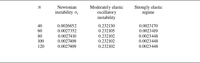
is reported in table 1. For
 $N \geq 120$
, the critical growth rate converges to up to six significant figures, and the leading eigenvalue of the Newtonian fluid converges to five significant figures; this resolution is used for all results reported in this paper.
Convergence of the leading eigenvalue with the Chebyshev order
 $N$
.

Table 1. Long description
The table presents the convergence of the leading eigenvalue with the Chebyshev order for three cases: Newtonian instability, moderately elastic oscillatory instability, and strongly elastic regime. It has four rows and three columns. The columns are labeled N, Newtonian instability σ_r, Moderately elastic oscillatory instability, and Strongly elastic regime. The rows are labeled with values for N: 40, 60, 80, 100, and 120. Each row contains corresponding values for the three cases. For example, Row 1: N, 40; Newtonian instability σ_r, 0.0026852; Moderately elastic oscillatory instability, 0.232130; Strongly elastic regime, 0.0023170.
To assess the quantitative accuracy, we reproduce the benchmark case of Zhang et al. (Reference Zhang, Lashgari, Zaki and Brandt2013) for comparison. The configuration is viscoelastic plane Poiseuille flow with
 $\beta = 0.5$
,
 $\textit{Wi} = 3.96$
,
 $C = 50$
,
 $\textit{Fe} = 10^{4}$
,
 $Re = 3960$
. At
 $N = 120$
, the present solver gives
 $\omega = 0.34089441 + 1.988801\times 10^{-7}\mathrm{i}$
, whereas the result of Zhang et al. (Reference Zhang, Lashgari, Zaki and Brandt2013) is
 $\omega = 0.34089441 + 1.988772\times 10^{-7}\mathrm{i}$
. A good agreement is readily seen and the accuracy of the solver is verified.
Variation of the critical parameters with
 $\textit{Wi}$
: (a) critical electric Rayleigh number
 $T_c$
; (b) critical oscillation frequency
 $\omega _c$
; (c) critical wavenumber
 $k_c$
. In panels (a) and (b), the red curves represent the reduced analytical predictions obtained from (3.3)–(3.6), while the black curves represent the results of the full Chebyshev spectral calculations. Panel (c) shows the critical wavenumber obtained from the full Chebyshev spectral calculations. All results are obtained for
 $\beta =0.9$
,
 $M=10$
,
 $C=10$
and
 $\textit{Fe}=10^{4}$
.

4.3. Comparison between numerical and analytical results
Figure 1 shows the variation of the critical electric Rayleigh number, the critical oscillation frequency and the critical wavenumber
 $k_{c}$
with
 $\textit{Wi}$
, for
 $\beta = 0.9$
,
 $M = 10$
,
 $C = 10$
,
 $\textit{Fe} = 10^{4}$
. The values
 $C=10$
,
 $M=10$
and
 $\textit{Fe}=10^4$
define a canonical strong-injection, drift-dominated benchmark widely used for unipolar electroconvection, while
 $\beta =0.9$
corresponds to a moderate polymeric viscosity fraction of
 $1-\beta =0.1$
. Here,
 $T_c$
exhibits a three-stage variation with
 $\textit{Wi}$
. To permit a direct comparison using the same physical variables, figures 1(a) and 1(b) now superpose the Chebyshev results and the reduced predictions of (3.3)–(3.6) over
 $0.2\leq \textit{Wi}\leq 1000$
. For
 $\beta =0.9$
and
 $\kappa =752.168$
, the reduced model predicts
 $\textit{Wi}_H=2.1791$
and a frequency maximum at
 $\textit{Wi}_{\textit{peak}}=4.3581$
, with
 $\omega _{c,\textit{peak}}=0.24187$
. The Chebyshev solution becomes oscillatory between
 $\textit{Wi}=2$
and
 $2.2$
and reaches its maximum between
 $\textit{Wi}=4$
and
 $5$
.
In the weakly elastic regime
 $\textit{Wi} \leq 1$
, elastic effects are negligible and the system behaves essentially as a Newtonian fluid. This is a stationary instability stage, with the critical value held near
 $163.90$
. In the transitional regime
 $1 \leq \textit{Wi} \leq 10$
, the critical value drops sharply as elasticity increases – an oscillatory instability stage. Here,
 $\textit{Wi}$
passes from negligible to dominant. The elastic relaxation time becomes comparable to the characteristic time of electroconvection, the two coupling on the same time scale to act jointly on the system, and the instability threshold becomes sensitive to
 $\textit{Wi}$
. The critical frequency reaches its peak value
 $\omega _{c} \approx 0.24$
at
 $\textit{Wi} \approx 5$
. In the strongly elastic regime
 $\textit{Wi} \geq 100$
, the critical value levels off onto a plateau and approaches the frozen-elasticity limit
 $\beta T_{c}^{N} = 147.5$
, while the critical frequency decreases monotonically with increasing
 $\textit{Wi}$
. Physically, the frozen-elasticity limit corresponds to
 $\hat \omega =\omega _c\textit{Wi}\gg 1$
, for which polymer relaxation is too slow over an oscillation cycle; the polymer response becomes predominantly elastic and its in-phase dissipative contribution vanishes, so that
 $\mu _{\textit{eff}}\to \beta$
and
 $T_c\to \beta T_c^N$
. Notably, the critical wavenumber remains close to
 $5.115$
over the entire range of
 $\textit{Wi}$
(varying by less than
 $0.1\,\%$
), indicating that elasticity markedly alters the threshold and oscillatory character of the instability, but not the spatial size of the convection cells.
Previous studies of viscoelastic electrohydrodynamic instability have largely been confined to the weak and moderately elastic regime,
 $\textit{Wi} = \mathcal{O}(10)$
. Through the order reduction of the equations and the mode selection algorithm, the present work extends the study of
 $\textit{Wi}$
to the strongly elastic regime,
 $\textit{Wi} = \mathcal{O}(10^{3})$
, and reveals the existence of a frozen-elasticity plateau in the critical value as
 $\textit{Wi}$
increases, together with its asymptotic approach to the frozen-elasticity limit
 $\beta T_{c}^{N}$
. The present work provides the first identification and characterisation of a frozen-elasticity limit for the linear onset of unipolar-injection electroconvection in a quiescent viscoelastic dielectric liquid.
The behaviour of the critical electric Rayleigh number
 $T_{c}$
and the critical oscillation frequency
 $\omega _{c}$
with
 $\textit{Wi}$
described already is quantitatively reproduced by the neutral solution (3.6). The single geometric constant
 $\kappa$
takes the value
 $752.2$
at
 $\beta = 0.9$
,
 $M = 10$
,
 $C = 10$
,
 $\textit{Fe} = 10^{4}$
and
 $\textit{Wi} = 100$
. This value is subsequently held fixed for all the remaining combinations of
 $\beta$
and
 $\textit{Wi}$
. Equation (3.6) predicts the dimensionless frequency (
 $\widehat {\omega }^{2} = (\omega _{c}\textit{Wi})^{2}$
) for sixteen data points spanning solvent ratios
 $\beta = 0.95, 0.9, 0.8, 0.7$
and more than one decade of
 $\textit{Wi}$
(
 $\textit{Wi} = 20, 50, 100, 200$
), compared with the numerical solution; the mean error is
 $0.1\,\%$
and the maximum
 $0.3\,\%$
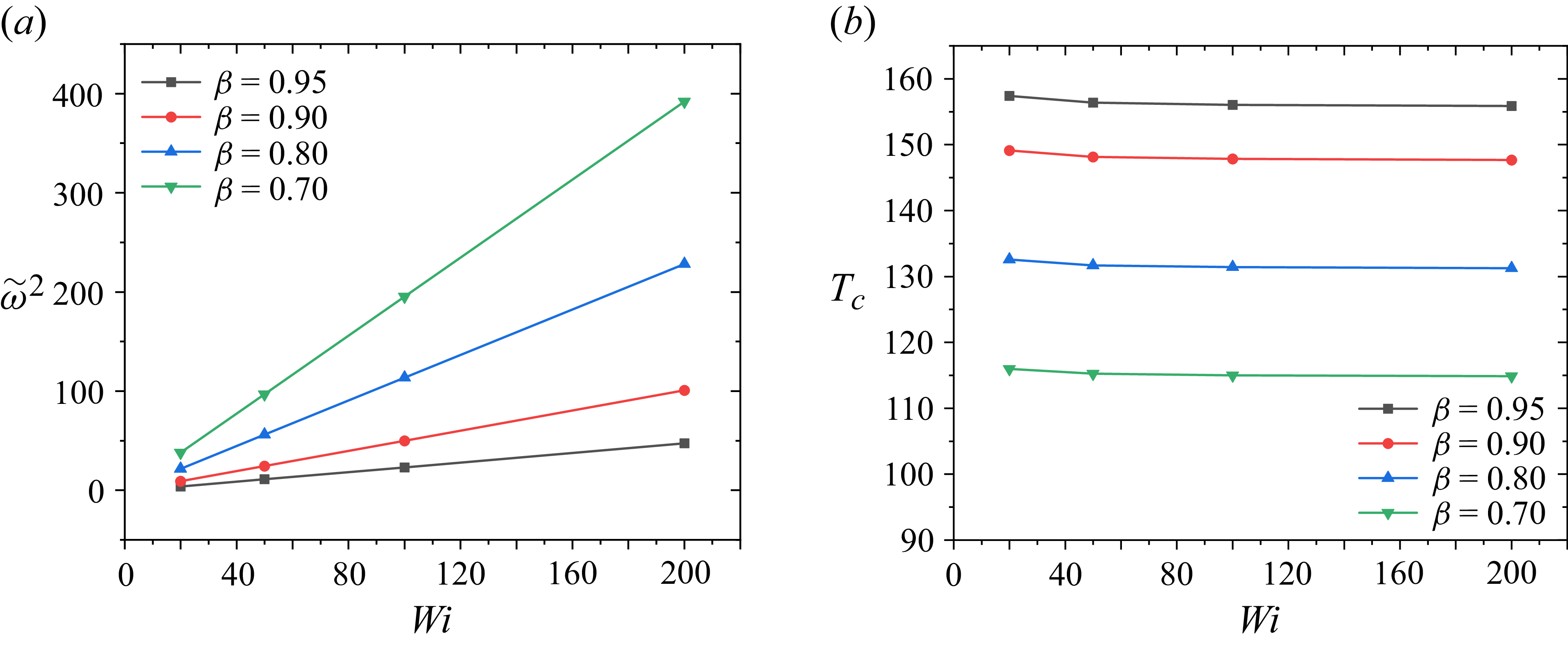
(figure 2
a). The corresponding critical electric Rayleigh number, predicted by (3.4), agrees with a mean error of
 $0.04\,\%$
and a maximum of
 $0.2\,\%$
(figure 2
b). (A point-by-point comparison of the sixteen numerical and analytical values is given in Appendix A.)
Analytical solution for the dimensionless frequency and the critical electric Rayleigh number: (a) dimensionless frequency predicted by (3.6); (b) critical electric Rayleigh number predicted by (3.4).

Figure 2. Long description
Panel A: A line graph shows the dimensionless frequency predicted by equation 3.6. The x-axis represents Wi, ranging from 0 to 200. The y-axis represents the dimensionless frequency squared, ranging from 0 to 400. Four lines are plotted for different beta values: 0.95 (black squares), 0.90 (red circles), 0.80 (blue triangles), and 0.70 (green inverted triangles). The lines show an increasing trend in dimensionless frequency with increasing Wi, with higher beta values resulting in lower frequencies. Panel B: Another line graph shows the critical electric Rayleigh number predicted by equation 3.4. The x-axis represents Wi, ranging from 0 to 200. The y-axis represents the critical electric Rayleigh number, ranging from 90 to 160. Four lines are plotted for different beta values: 0.95 (black squares), 0.90 (red circles), 0.80 (blue triangles), and 0.70 (green inverted triangles). The lines show a slight decrease in the critical electric Rayleigh number with increasing Wi, with higher beta values resulting in higher critical electric Rayleigh numbers.
Comparison of the analytical and numerical results for the coefficients of the scaling laws (3.8) and (3.9): (a) coefficient
 $A(\beta )$
of the frequency scaling law (3.8); (b) coefficient
 $a(\beta )$
of the threshold scaling law (3.9); (c) back-calculated effective coefficient
 $\kappa$
as a function of
 $\beta$
. The numerical coefficients in panels (a) and (b) are obtained by averaging the rescaled Chebyshev results over
 $\textit{Wi}=20$
,
 $50$
,
 $100$
and
 $200$
; the same values of
 $\textit{Wi}$
are used to examine the weak parameter dependence of
 $\kappa$
in panel (c).

The analytical solution is entirely independent of the numerical computation and the mean error between them does not exceed
 $0.1\,\%$
; this constitutes a two-way validation: the high resolution spectral method confirms the correctness of the analytical theory, while the analytical solution conversely confirms the low error of the numerical solver. In the limit
 $\textit{Wi} \to \infty$
, (3.6) yields the two scaling laws (3.8) and (3.9). Figure 3(a) compares the coefficient of the frequency scaling law (3.8) obtained from the analytical theory with that obtained from a numerical fit, where the fitted coefficient is the average over the values
 $\textit{Wi}$
(
 $20, 50, 100, 200$
) used in this work. These values collectively sample the approach to and establishment of the frozen-elasticity plateau, which is fully developed for
 $\textit{Wi}\gt 100$
according to figure 1(a). Smaller values of
 $\textit{Wi}$
are excluded because the large-
 $\textit{Wi}$
scaling laws are then inapplicable, particularly because the
 $-1$
term in (3.6) cannot be neglected. This subset was selected to characterise the strongly elastic trend: figure 1(a) shows that the threshold has essentially approached its plateau for
 $\textit{Wi}\gtrsim 100$
, and
 $\textit{Wi}=200$
provides a representative point beyond the beginning of this plateau. Because the derivation of the scaling law (3.8) assumes large
 $\textit{Wi}$
and neglects the
 $-1$
term in the analytical solution (3.6), this term is not negligible at smaller
 $\textit{Wi}$
(
 $\textit{Wi} = 20$
); the analytical and numerical solutions therefore differ and this discrepancy increases markedly with
 $\beta$
(as
 $\beta$
increases, the polymeric viscosity fraction
 $1-\beta$
and
 $\hat {\omega }$
decrease, so the influence of the neglected term becomes more pronounced). Figure 3(b) compares the analytical and numerical results for the coefficient
 $a(\beta )$
of the asymptotic threshold scaling law (3.9). The two curves vary with the same slope, showing that the main trend of the derived theory is correct; however, the numerical result is consistently and appreciably larger than the analytical one, and this gap widens as
 $\beta$
decreases. The origin of this behaviour is that, in the derivation,
 $\kappa$
was assumed to be a fixed shape constant, neglecting the weak dependence of
 $\kappa$
on the deformation of the eigenfunction with
 $\beta$
; this is a secondary effect of eigenfunction deformation, and the present derivation is given only with this effect neglected. Figure 3(c) shows the weak dependence of the Newtonian-based geometric coefficient
 $\kappa$
on
 $\beta$
and
 $\textit{Wi}$
. For each of the sixteen combinations of
 $\beta =0.70$
,
 $0.80$
,
 $0.90$
and
 $0.95$
, and
 $\textit{Wi}=20$
,
 $50$
,
 $100$
and
 $200$
,
 $\kappa$
is evaluated by inverting (3.6) using the corresponding frequency obtained from the full spectral calculation. The resulting values remain within
 \begin{align} 750.038 \leq \kappa \leq 753.309. \end{align}
The representative value used throughout the reduced analytical model is
 $\kappa =752.168$
, rounded to
 $752.2$
, which is determined at
 $\beta =0.9$
and
 $\textit{Wi}=100$
. We find that, for
 $\beta \to 0$
, neglecting this effect leads to a discrepancy of approximately
 $15.9$
between theory and computation. A check confirms that
 $a(\beta )A(\beta )^{2} = 163.902$
holds identically, demonstrating the intrinsic self-consistency of the scaling laws (3.8) and (3.9).
5. Conclusions
Within the framework of electrohydrodynamics, this paper has presented a linear stability analysis of the convective instability of a quiescent Oldroyd-B viscoelastic fluid under an electric field, providing the first analytical theory for the oscillatory onset of this problem. The main conclusions are as follows.
-
(i) By exploiting the properties of the linearised constitutive relation under a quiescent base state, a closed-form approximate analytical solution is obtained. The central result is the analytical neutral oscillation solution (3.6). In the large-
 $\textit{Wi}$
limit, asymptotic scaling laws for the dimensionless frequency and the critical electric Rayleigh number, (3.8) and (3.9), are obtained. The two asymptotic scaling laws are found to share the same mechanism, with their coefficients satisfying the self-consistency relation (3.10).
-
(ii) The critical electric Rayleigh number exhibits a pronounced three-stage structure with
$\textit{Wi}$
, dividing the behaviour into three regimes. The transition at
$\textit{Wi}=\textit{Wi}_{\mathrm H}$
marks the onset of overstability, in which the polymer-relaxation-induced phase lag changes the primary instability from a stationary mode to a Hopf mode. The linear stability analysis of viscoelastic electroconvective instability is extended into the strongly elastic regime, up to
$\textit{Wi} = 10^{3}$
, fully characterising the frozen-elasticity plateau and its asymptotic behaviour, which had not previously been systematically revealed in the electroconvection configuration. -
(iii) Mutual corroboration of theory and computation. The approximate analytical solution is obtained entirely independently of the numerical computation, with a single geometric constant as input. It predicts the critical threshold and frequency across four solvent ratios and one decade of
$\textit{Wi}$
, with a maximum error of no more than
$0.3\,\%$
. The quantitative agreement between these two independent approaches provides a twofold confirmation of the reliability of the results.


The analytical framework established here shows that the quiescent base-state configuration of electroconvection allows the viscoelastic oscillatory instability problem to be reduced to a closed, solvable form, yielding the threshold and frequency scaling laws together with their self-consistency relation.
This solvability provides a benchmark against which the possibility of an analytical treatment can be tested in future configurations involving a base flow, multipolar injection or curved electrodes, and it offers a clear criterion for experimental studies of electrohydrodynamic behaviour in the strongly elastic regime.
Funding
This work was supported by the National Natural Science Foundation of China (grant number 12172110).
Declaration of interests
The authors report no conflict of interest.
Data availability statement
The data that support the findings of this study are available from the corresponding author upon reasonable request.
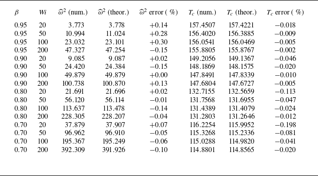
Appendix A. Numerical and analytical comparison
Detailed comparisons between the full Chebyshev spectral calculations and the reduced analytical solutions are presented here for the parameter sets considered in this study. In table 2, ‘num.’ denotes the full Chebyshev results, whereas ‘theor.’ denotes the corresponding reduced solutions evaluated from (3.4) and (3.6), with their complete finite-
 $\textit{Wi}$
dependence retained.
Comparison of the numerical and analytical solutions of (3.6) and (3.4) at the sixteen discrete points
 $(\beta , \textit{Wi})$
, with relative errors.

Table 2. Long description
The table presents a comparison between numerical and theoretical solutions for various parameter sets. It has 12 rows and 7 columns. The columns are labeled as follows: beta, Wi, omega squared (num.), omega squared (theor.), omega squared error (percent), T subscript c (num.), T subscript c (theor.), and T subscript c error (percent). The rows list different values for these parameters. For example, Row 1: beta 0.95, Wi 20, omega squared (num.) 3.773, omega squared (theor.) 3.778, omega squared error 0.14 percent, T subscript c (num.) 157.4507, T subscript c (theor.) 157.4221, T subscript c error 0.018 percent.
 N

 Wi
 Tc
 ωc
 kc
 β=0.9
 M=10
 C=10
 Fe=104

 A(β)
 a(β)
 κ
 β
 Wi=20
 50
 100
 200
 Wi
 κ
 (β,Wi)


