1 Introduction
The technique of hydraulic fracturing is mainly used as a well stimulation technique in unconventional reservoirs, which have relatively low permeability and porosity, making it difficult to extract oil and gas (Economides & Nolte Reference Economides and Nolte2000). The creation of fractures in rock formations increases the surface area connected to the wellbore, allowing larger amounts of hydrocarbons to be released. Other applications include measurement of existing (in situ) stresses (Fairhurst Reference Fairhurst1964), carbon sequestration (Rudnicki Reference Rudnicki2000; Huppert & Neufeld Reference Huppert and Neufeld2014), geothermal energy reservoirs (Murphy et al. Reference Murphy, Tester, Grigsby and Potter1981), compensation grouting (Mair & Hight Reference Mair and Hight1994) and disposal of toxic liquid waste deep underground. Fluid-driven fracturing is also encountered in nature when studying magma transport (Lister & Kerr Reference Lister and Kerr1991). In this last case, the mechanism for crack propagation of magma-driven dykes is the pressure caused by density differences between the fluid and the surrounding rock formation.
Hydraulic fracturing in its most simple form, a single crack, is still very complicated to model, as it involves the coupling of at least three processes, namely (i) mechanical deformation of the fracture surfaces by fluid pressure, (ii) fluid flow in the fracture and (iii) fracture propagation. These processes are usually modelled by (i) the theory of linear elasticity, (ii) lubrication theory and (iii) linear elastic fracture mechanics (LEFM), respectively.
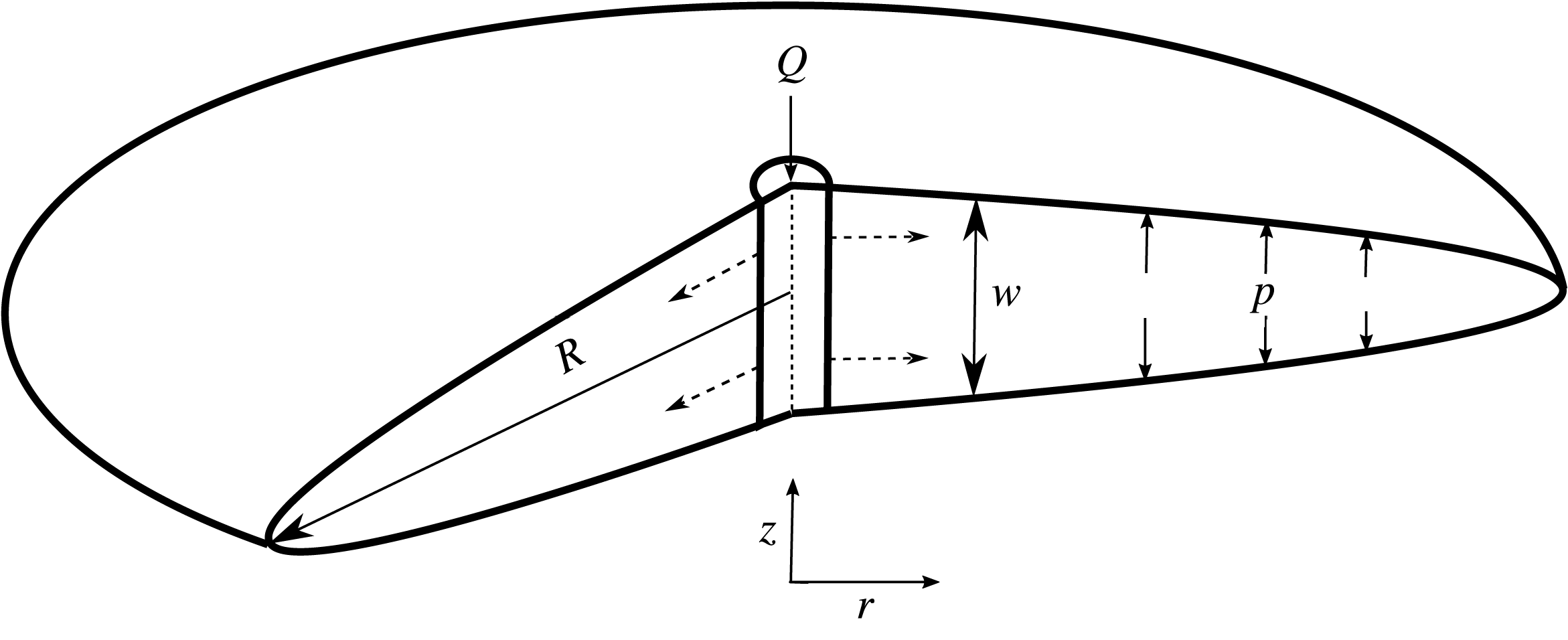
Schematic diagram showing the radial fracture geometry.

The radial fracture geometry that we discuss here applies to homogeneous formation conditions, where the injection region is modelled as a point source (figure 1). This occurs when the wellbore from which fluid is injected is orientated perpendicular to the direction of maximum confining stress, or when fluid is injected radially into a medium that can be considered homogeneous and infinite in comparison with the size of the fracture.
The radial model, or penny-crack problem, has been studied extensively since the work of Sneddon (Reference Sneddon1946). Initially, a theory was developed for hydraulic fractures in an infinite medium assuming that viscous dissipation within the fluid was the dominant mechanism for energy dissipation (Spence & Sharp Reference Spence and Sharp1985). Since then, Garagash and others have focused on the crack tip region (Garagash & Detournay Reference Garagash and Detournay2000; Garagash, Detournay & Adachi Reference Garagash, Detournay and Adachi2011). They have also shown that two dissipative processes, fracturing of the rock (toughness) and viscous flow in the fracture, along with two fluid balance mechanisms, leak-off and storage of fracturing fluid in the fracture, significantly affect the fracture propagation behaviour (Savitski & Detournay Reference Savitski and Detournay2002; Detournay & Garagash Reference Detournay and Garagash2003).
Experiments that have tried to capture these dynamics have involved materials such as gelatin and polymethyl methacrylate (PMMA), which have been widely used to model geological mechanics because they exhibit elastic and brittle behaviour similar to that seen in rocks (Takada Reference Takada1990; Alpern et al. Reference Alpern, Marone, Elsworth, Belmonte and Connelly2012). Hubbert & Willis (Reference Hubbert and Willis1957) investigated the elastic field around an injection point and its influence on fracture orientation using gelatin and focusing on early fracture formation, finding that fractures should be perpendicular to the axis of least stress. Bunger & Detournay (Reference Bunger and Detournay2008) developed a novel experiment to measure the aperture of a fluid-driven fracture between two PMMA plates glued together with an adhesive. This experiment validated theoretical expectations for the crack tip region when the dominant mechanism for energy dissipation was either toughness (crack tip extension) or viscous flow. Recently, Lai et al. (Reference Lai, Zheng, Dressaire, Wexler and Stone2015) and Lai et al. (Reference Lai, Zheng, Dressaire and Stone2016) conducted experiments using gelatin, which validated scaling laws of the time dependence of crack growth and aperture in the viscous and toughness regimes.
Our study follows a similar experimental set-up to that reported in the papers of Lai et al. (Reference Lai, Zheng, Dressaire, Wexler and Stone2015, Reference Lai, Zheng, Dressaire and Stone2016). The work described here was conducted concurrently with those studies and not inspired as a result of their work. However, the dynamic scaling results produced here do serve as an exploration and confirmation of their results in another medium, cross-linked hydrogel. Moreover, our study focuses on the transition between the viscous and toughness regimes identified by Bunger & Detournay (Reference Bunger and Detournay2008) and Lai et al. (Reference Lai, Zheng, Dressaire, Wexler and Stone2015, Reference Lai, Zheng, Dressaire and Stone2016). Here, we report a better experimental agreement with the toughness scaling prediction, and also rule out possible experimental reasons for the underprediction of the fracture growth in the viscosity regime compared with theory, which has also been seen in gelatin. Using novel particle image velocimetry (PIV) measurements of the flow inside the fracture, we also observe the evolving flow structure. These velocity measurements may provide new insights into the transport of proppants within fractures.
In this paper, we set out to verify the time-dependent radial and aperture fracture scalings outlined in Savitski & Detournay (Reference Savitski and Detournay2002) for an impermeable medium. We will also analyse the time-dependent crack tip behaviour of these fractures to further characterise the two dominant regimes, toughness or viscous, and the transition between them. Finally, we report on the fluid flow within these fractures and the differences in the flow structure in the two regimes of propagation. In § 2, we introduce this model; § 3 describes the hydrogel properties and § 4 the experimental set-up. The experimental results are presented and compared with the theoretical models in § 5 and our conclusions are given in § 6.
2 The model
In this section, we review and discuss the existing mathematical models in order to motivate our experimental approach and illustrate the important physical mechanisms involved. This theoretical framework was first introduced by Spence & Sharp (Reference Spence and Sharp1985) and Savitski & Detournay (Reference Savitski and Detournay2002).
We consider a radial fracture propagating into an impermeable elastic solid (figure 1), in which the leak-off of the fracturing fluid into the medium is considered to be negligible. The fracture is driven by a constant volumetric injection rate
 $Q$
of an incompressible fluid with dynamic viscosity
 $\unicode[STIX]{x1D707}$
. The elastic medium is characterised by Young’s modulus
 $E$
, Poisson’s ratio
 $\unicode[STIX]{x1D708}$
and toughness
 $K_{IC}$
. The following assumptions are then used to simplify the problem: (i) there is no fluid lag (i.e. the fluid front coincides with the fracture front); (ii) LEFM and lubrication theory for the fluid flow are applicable; (iii) the wellbore (injection) radius is negligible compared with the radius of the fracture (i.e. it can be modelled as a point source); (iv) the fracture propagates continuously in a mobile equilibrium.
2.1 Mathematical formulation
By applying these assumptions we can formulate the problem to find the crack aperture width
 $w(r,t)$
, the fracture radius
 $R(t)$
and the net pressure
 $p(r,t)$
.
2.1.1 Linear elasticity
We define the net pressure
 $p(r,t)=-\unicode[STIX]{x1D70E}_{zz}$
through the stress tensor
 $\unicode[STIX]{x1D748}$
, i.e. the normal traction. Based on linear elasticity, the mechanical deformation of the elastic matrix is given by the integral relation, which relates the net pressure
 $p(r,t)$
and the crack aperture
 $w(r,t)$
(Sneddon Reference Sneddon1951; Spence & Sharp Reference Spence and Sharp1985),
 $$\begin{eqnarray}p(r,t)=-E^{\prime }\int _{0}^{R(t)}\frac{\unicode[STIX]{x2202}w(s,t)}{\unicode[STIX]{x2202}s}M\left(\frac{r}{s}\right)\frac{\text{d}s}{s},\end{eqnarray}$$
where
 $E^{\prime }$
is the plane strain modulus, which can be expressed in terms of
 $E$
and
 $\unicode[STIX]{x1D708}$
as
 $E^{\prime }=E/(1-\unicode[STIX]{x1D708}^{2})$
, and
 $M(\cdot )$
is the elasticity kernel,
 $$\begin{eqnarray}M\left(\frac{r}{s}\right)=\left\{\begin{array}{@{}ll@{}}\displaystyle \frac{2s^{2}}{\unicode[STIX]{x03C0}(s^{2}-r^{2})}E\left(\frac{r}{s}\right),\quad & r<s,\\ \displaystyle \frac{2rs}{\unicode[STIX]{x03C0}(s^{2}-r^{2})}E\left(\frac{s}{r}\right)+\frac{s}{r}K\left(\frac{s}{r}\right),\quad & s<r,\end{array}\right.\end{eqnarray}$$
where
 $E(\cdot )$
and
 $K(\cdot )$
are elliptic integrals of the first and second kind. Inversion of (2.1) gives rise to the following double integral expression for the elastic response to pressure (Sneddon & Lowengrub Reference Sneddon and Lowengrub1969),
 $$\begin{eqnarray}w(r,t)=\frac{8R}{\unicode[STIX]{x03C0}E^{\prime }}\int _{r/R}^{1}\frac{\unicode[STIX]{x1D709}}{\sqrt{\unicode[STIX]{x1D709}^{2}-(r/R)^{2}}}\int _{0}^{1}\frac{xp(x\unicode[STIX]{x1D709}R,t)}{\sqrt{1-x^{2}}}\,\text{d}x\,\text{d}\unicode[STIX]{x1D709}.\end{eqnarray}$$
2.1.2 Lubrication theory
The flow of fluid in the crack is modelled using lubrication theory under the assumption that
 $$\begin{eqnarray}w(r,t)\ll R(t),\end{eqnarray}$$
which is clearly evident in our experiments, except at the initiation of the crack. For this theory to be valid, it is also required that
 $$\begin{eqnarray}Re=\unicode[STIX]{x1D6FC}\frac{\unicode[STIX]{x1D70C}Uw}{\unicode[STIX]{x1D707}}=\frac{w}{R}\frac{\unicode[STIX]{x1D70C}Uw}{\unicode[STIX]{x1D707}}=\frac{\unicode[STIX]{x1D70C}Qw}{2\unicode[STIX]{x03C0}R^{2}\unicode[STIX]{x1D707}}\ll 1,\end{eqnarray}$$
where
 $Re$
is the Reynolds number,
 $\unicode[STIX]{x1D6FC}$
is the aspect ratio of the fracture and
 $U$
is the velocity scale of the fluid of density
 $\unicode[STIX]{x1D70C}$
and dynamic viscosity
 $\unicode[STIX]{x1D707}$
.
A fluid mass balance gives
 $$\begin{eqnarray}\frac{\unicode[STIX]{x2202}w(r,t)}{\unicode[STIX]{x2202}t}+\frac{1}{r}\frac{\unicode[STIX]{x2202}}{\unicode[STIX]{x2202}r}(rq(r,t))=0,\end{eqnarray}$$
where
 $q(r,t)$
is the radial flow rate, and using the Poiseuille law, we obtain
 $$\begin{eqnarray}q(r,t)=-\frac{w^{3}}{12\unicode[STIX]{x1D707}}\frac{\unicode[STIX]{x2202}p(r,t)}{\unicode[STIX]{x2202}r}.\end{eqnarray}$$
By combining (2.6) and (2.7), we obtain a second nonlinear differential equation (Batchelor Reference Batchelor1967), known as Reynolds equation, which relates the aperture width to the pressure,
 $$\begin{eqnarray}\frac{\unicode[STIX]{x2202}w(r,t)}{\unicode[STIX]{x2202}t}=\frac{1}{12\unicode[STIX]{x1D707}}\frac{1}{r}\frac{\unicode[STIX]{x2202}}{\unicode[STIX]{x2202}r}\left(rw^{3}(r,t)\frac{\unicode[STIX]{x2202}p}{\unicode[STIX]{x2202}r}\right).\end{eqnarray}$$
2.1.3 Linear elastic fracture mechanics
The fracture propagation criterion is based on LEFM. The main assumption of LEFM is that the region near the fracture tip where the behaviour of the medium is not elastic, but undergoes plastic deformation or microcracking, is small compared with the crack size. LEFM implies that a fracture will propagate if the mode I (tensile crack) stress intensity factor
 $K_{I}$
exceeds the material toughness
 $K_{IC}$
. Therefore, the fracture propagation criterion can be written as (Kanninen & Popelar Reference Kanninen and Popelar1985)
 $$\begin{eqnarray}K_{I}=K_{IC},\end{eqnarray}$$
where
 $$\begin{eqnarray}K_{IC}=\sqrt{2\unicode[STIX]{x1D6FE}_{s}E^{\prime }}.\end{eqnarray}$$
Here,
 $K_{IC}$
is a material property called the fracture toughness and
 $\unicode[STIX]{x1D6FE}_{s}$
is the fracture surface energy of the elastic medium, which can be defined as the energy required to create one unit of surface area. The stress intensity factor
 $K_{I}$
predicts the stress state near the tip of a crack. For the penny-shaped fracture, this takes the form (Rice Reference Rice1968)
 $$\begin{eqnarray}K_{I}=\frac{2}{\sqrt{\unicode[STIX]{x03C0}R}}\int _{0}^{R(t)}\frac{p(r,t)}{\sqrt{R^{2}-r^{2}}}r\,\text{d}r.\end{eqnarray}$$
2.1.4 Boundary conditions
The tip boundary conditions are set by a zero-fracture aperture at the tip,
 $$\begin{eqnarray}w=0,\quad r=R(t),\end{eqnarray}$$
and a no flow condition,
 $q(R)=0$
. Then, using Poiseuille’s law (2.7), we derive
 $$\begin{eqnarray}w^{3}(r,t)\frac{\unicode[STIX]{x2202}p(r,t)}{\unicode[STIX]{x2202}r}=0,\quad r=R(t).\end{eqnarray}$$
Using mass balance, we obtain the following relationship between the flow rate
 $q(r,t)$
and the constant injection rate
 $Q$
 $$\begin{eqnarray}2\unicode[STIX]{x03C0}\lim _{r\rightarrow 0}rq(r,t)=Q.\end{eqnarray}$$
Global mass balance is also used in the form
 $$\begin{eqnarray}Qt=2\unicode[STIX]{x03C0}\int _{0}^{R(t)}rw(r,t)\,\text{d}r.\end{eqnarray}$$
This set of equations, combining elasticity (2.3), lubrication theory (2.8), LEFM (2.9), (2.11), inlet conditions (2.14) or (2.15) and tip boundary conditions (2.12) or (2.13), forms a system that can be solved for
 $w(r,t)$
,
 $p(r,t)$
and
 $R(t)$
.
From this system of equations, we can construct two distinct regimes of fracture propagation using elasticity (2.3), lubrication theory (2.8), LEFM (2.11) and global mass balance (2.15). The viscosity- and toughness-dominated regimes will arise from neglecting material toughness (LEFM) (2.11) and viscous fluid flow (2.8), respectively.
2.2 Scaling
We non-dimensionalise these equations using
 $R=R_{0}\hat{R}$
,
 $t=t_{0}\hat{t}$
, etc., where
 $R_{0},t_{0},\ldots$
are characteristic scales. The material parameters of viscosity
 $\unicode[STIX]{x1D707}^{\prime }$
and toughness
 $K^{\prime }$
are defined in order to simplify the process (Savitski & Detournay Reference Savitski and Detournay2002), as
 $$\begin{eqnarray}\unicode[STIX]{x1D707}^{\prime }=12\unicode[STIX]{x1D707},\quad K^{\prime }=4\left(\frac{2}{\unicode[STIX]{x03C0}}\right)^{1/2}K_{Ic}.\end{eqnarray}$$
The system of equations is then transformed as follows.
(i) Linear elasticity, (2.3)
(2.17) $$\begin{eqnarray}{\hat{w}}=\frac{8}{\unicode[STIX]{x03C0}}\frac{p_{0}R_{0}\hat{R}}{w_{0}E^{\prime }}\int _{\hat{r}/\hat{R}}^{1}\frac{\unicode[STIX]{x1D709}}{\sqrt{\unicode[STIX]{x1D709}^{2}-(\hat{r}/\hat{R})^{2}}}\int _{0}^{1}\frac{x\hat{p}}{\sqrt{1-x^{2}}}\,\text{d}x\,\text{d}\unicode[STIX]{x1D709}.\end{eqnarray}$$
(ii) Lubrication theory, (2.8)
(2.18)$$\begin{eqnarray}\frac{\unicode[STIX]{x2202}{\hat{w}}}{\unicode[STIX]{x2202}\hat{t}}=\frac{t_{0}w_{0}^{2}p_{0}}{\unicode[STIX]{x1D707}^{\prime }R_{0}^{2}}\frac{1}{\hat{r}}\frac{\unicode[STIX]{x2202}}{\unicode[STIX]{x2202}\hat{r}}\left(\hat{r}{\hat{w}}^{3}\frac{\unicode[STIX]{x2202}\hat{p}}{\unicode[STIX]{x2202}\hat{r}}\right).\end{eqnarray}$$
- (2.19)$$\begin{eqnarray}\frac{K^{\prime }}{p_{0}R_{0}^{1/2}}=\frac{2^{7/2}}{\unicode[STIX]{x03C0}\sqrt{\hat{R}}}\int _{0}^{\hat{R}}\frac{\hat{p}}{\sqrt{\hat{R}^{2}-\hat{r}^{2}}}\hat{r}\,\text{d}\hat{r}.\end{eqnarray}$$
(iv) Global mass balance, (2.15)
(2.20)$$\begin{eqnarray}\hat{Q}\hat{t}=2\unicode[STIX]{x03C0}\frac{R_{0}^{2}w_{0}}{Q_{0}t_{0}}\int _{0}^{\hat{R}}\hat{r}{\hat{w}}\,\text{d}\hat{r}.\end{eqnarray}$$


We then set the dimensionless groups in (2.17), (2.18), (2.19) and (2.20) to one respectively,
 $$\begin{eqnarray}\displaystyle & \displaystyle \frac{R_{0}p_{0}}{w_{0}E^{\prime }}=1, & \displaystyle\end{eqnarray}$$
 $$\begin{eqnarray}\displaystyle & \displaystyle \frac{t_{0}w_{0}^{2}p_{0}}{\unicode[STIX]{x1D707}^{\prime }R_{0}^{2}}=1, & \displaystyle\end{eqnarray}$$
 $$\begin{eqnarray}\displaystyle & \displaystyle \frac{K^{\prime }}{p_{0}R_{0}^{1/2}}=1, & \displaystyle\end{eqnarray}$$
 $$\begin{eqnarray}\displaystyle & \displaystyle \frac{R_{0}^{2}w_{0}}{Q_{0}t_{0}}=1. & \displaystyle\end{eqnarray}$$
Using these dimensionless groups, we introduce the viscosity- and toughness-dominated scalings, denoting them with subscripts
 $m$
and
 $k$
, respectively. From this, we can also identify the values of the scales,
 $$\begin{eqnarray}R_{0}=\frac{\unicode[STIX]{x1D707}^{\prime }Q_{0}{E^{\prime }}^{3}}{{K^{\prime }}^{2}},\quad w_{0}=\left(\frac{\unicode[STIX]{x1D707}^{\prime }Q_{0}E^{\prime }}{{K^{\prime }}^{2}}\right)^{1/2},\quad p_{0}=\left(\frac{{K^{\prime }}^{6}}{\unicode[STIX]{x1D707}^{\prime }Q_{0}{E^{\prime }}^{3}}\right)^{1/2},\quad t_{0}=\left(\frac{{\unicode[STIX]{x1D707}^{\prime }}^{5}Q_{0}^{3}{E^{\prime }}^{13}}{{K^{\prime }}^{18}}\right)^{1/2}\!.\end{eqnarray}$$
2.2.1 Viscosity scaling
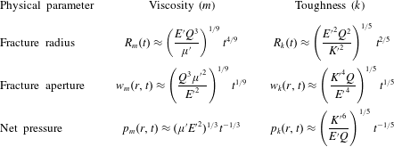
By combining groups from elasticity (2.21), lubrication theory (2.22) and mass balance (2.24), we arrive at the radial viscosity scaling, where
 $$\begin{eqnarray}R_{m}=\left(\frac{Q^{3}E^{\prime }t^{4}}{\unicode[STIX]{x1D707}^{\prime }}\right)^{1/9},\end{eqnarray}$$
upon dropping the non-dimensionalisation notation. From this scaling, we deduce the other viscosity-dominated scalings. For the fracture aperture it is
 $$\begin{eqnarray}w_{m}=\left(\frac{Q^{3}{\unicode[STIX]{x1D707}^{\prime }}^{2}t}{{E^{\prime }}^{2}}\right)^{1/9}\end{eqnarray}$$
and for the net pressure it is
 $$\begin{eqnarray}p_{m}=\left(\frac{\unicode[STIX]{x1D707}^{\prime }{E^{\prime }}^{2}}{t}\right)^{1/3},\end{eqnarray}$$
all of which are given in table 1.
Scaling relations for the time dependence of the toughness- and viscosity-dominated regimes.

Further, we define a dimensionless toughness
 ${\mathcal{K}}$
as in Savitski & Detournay (Reference Savitski and Detournay2002),
 $$\begin{eqnarray}{\mathcal{K}}=K^{\prime }\left(\frac{t_{0}^{2}}{{\unicode[STIX]{x1D707}^{\prime }}^{5}Q_{0}^{3}{E^{\prime }}^{13}}\right)^{1/18},\end{eqnarray}$$
so that the dimensionless propagation criterion (2.19) can be written as
 $$\begin{eqnarray}{\mathcal{K}}=\frac{2^{7/2}}{\unicode[STIX]{x03C0}\sqrt{\hat{R}}}\int _{0}^{\hat{R}}\frac{\hat{p}}{\sqrt{\hat{R}^{2}-\hat{r}^{2}}}\hat{r}\,\text{d}\hat{r}.\end{eqnarray}$$
Thus, in the viscosity scaling, the toughness
 ${\mathcal{K}}$
is the only parameter in the governing equations. In the viscosity-dominated regime,
 ${\mathcal{K}}$
is small, and, since
 ${\mathcal{K}}$
increases with time, the viscous regime will ultimately transition to the toughness regime.
2.2.2 Toughness scaling
For the toughness scaling, we combine elasticity (2.21), LEFM (2.23) and mass balance (2.24) to obtain the radial scaling,
 $$\begin{eqnarray}R_{k}=\left(\frac{Q^{2}{E^{\prime }}^{2}t^{2}}{{K^{\prime }}^{2}}\right)^{1/5}.\end{eqnarray}$$
Once again, this enables us to deduce the other toughness scalings for the fracture aperture,
 $$\begin{eqnarray}w_{k}=\left(\frac{{K^{\prime }}^{4}Qt}{{E^{\prime }}^{4}}\right)^{1/5},\end{eqnarray}$$
and the net pressure,
 $$\begin{eqnarray}p_{k}=\left(\frac{{K^{\prime }}^{6}}{E^{\prime }Qt}\right)^{1/5},\end{eqnarray}$$
as can be found in table 1.
Similarly, we define a natural choice for a dimensionless viscosity
 ${\mathcal{M}}$
,
 $$\begin{eqnarray}{\mathcal{M}}=\unicode[STIX]{x1D707}^{\prime }\left(\frac{Q_{0}^{3}{E^{\prime }}^{13}}{{K^{\prime }}^{18}t_{0}^{2}}\right)^{1/5},\end{eqnarray}$$
giving a lubrication equation (2.18) of the form
 $$\begin{eqnarray}{\mathcal{M}}\frac{\unicode[STIX]{x2202}{\hat{w}}}{\unicode[STIX]{x2202}\hat{t}}=\frac{1}{\hat{r}}\frac{\unicode[STIX]{x2202}}{\unicode[STIX]{x2202}\hat{r}}\left(\hat{r}{\hat{w}}^{3}\frac{\unicode[STIX]{x2202}\hat{p(r,t)}}{\unicode[STIX]{x2202}\hat{r}}\right).\end{eqnarray}$$
For the toughness-dominated regime,
 ${\mathcal{M}}$
is small, and, again, the fracture will be increasingly dominated by toughness at late times.
2.2.3 Transition
Noticing that the dimensionless viscosity
 ${\mathcal{M}}$
and toughness
 ${\mathcal{K}}$
are related by a simple power law,
 $$\begin{eqnarray}{\mathcal{K}}={\mathcal{M}}^{-5/18},\end{eqnarray}$$
the transition between the two regimes can be understood using a single parameter, which is chosen to be
 ${\mathcal{K}}$
. It is estimated from asymptotics and numerical simulations that a fracture propagates in the viscous regime when
 ${\mathcal{K}}\lesssim 1$
and in the toughness regime when
 ${\mathcal{K}}\gtrsim 3.5$
(Savitski & Detournay Reference Savitski and Detournay2002).
The transition and distinction between the two regimes can perhaps be more easily understood by the characteristic time scale
 $t_{0}$
from (2.25). This can also be constructed by equating the viscous and toughness length scales,
 $R_{m}=R_{k}$
. Solving for
 $t$
, we evaluate the characteristic time
 $t_{mk}$
it takes to transition from a viscous- to a toughness-dominated regime, where
 $$\begin{eqnarray}t_{mk}=\left(\frac{{\unicode[STIX]{x1D707}^{\prime }}^{5}Q^{3}{E^{\prime }}^{13}}{{K^{\prime }}^{18}}\right)^{1/2}\sim \left(\frac{\unicode[STIX]{x1D707}^{5}Q^{3}{E^{\prime }}^{13}}{{K_{IC}}^{18}}\right)^{1/2}.\end{eqnarray}$$
Therefore, for
 $t\ll t_{mk}$
, viscosity is the main source of energy dissipation, and for
 $t\gg t_{mk}$
, material toughness dominates.
Finally, this time scale conveniently relates back to the dimensionless toughness and viscosity parameters,
 $$\begin{eqnarray}{\mathcal{K}}={\mathcal{M}}^{-5/18}=\left(\frac{t}{t_{mk}}\right)^{1/9}.\end{eqnarray}$$
From the dimensionless parameters
 ${\mathcal{M}}$
and
 ${\mathcal{K}}$
, we can deduce that the fracture only transitions from a viscosity- to a toughness-dominated regime. This is due to the fact that as time evolves, the dimensionless viscosity
 ${\mathcal{M}}$
decreases and the dimensionless toughness
 ${\mathcal{K}}$
increases, because they are inversely related. Therefore, material toughness becomes increasingly significant as the fracture propagates.
2.3 Crack tip asymptotes
The solution near the crack tip is known to be characterised by a multiscale behaviour, which is related to the dominant energy dissipative processes that determine the length scales of the various tip asymptotes.
Linear elastic fracture mechanics provides the asymptotic condition on the crack aperture
 $w$
(Rice Reference Rice1968). This can be deduced from (2.3) by assuming that the pressure
 $p(r,t)=p_{s}(t)$
is only time-dependent in the toughness regime because the fluid flow within the crack is quasisteady, which gives the profile of the crack shape,
 $$\begin{eqnarray}w(r,t)=\frac{8R}{\unicode[STIX]{x03C0}E^{\prime }}p_{s}(t)\sqrt{1-\left(\frac{r}{R}\right)^{2}}.\end{eqnarray}$$
Using the stress intensity factor (2.11), we can relate the pressure
 $p_{s}(t)$
to the material toughness,
 $$\begin{eqnarray}K_{IC}=\frac{2p_{s}(t)\sqrt{R}}{\sqrt{\unicode[STIX]{x03C0}}}.\end{eqnarray}$$
By combining (2.39) and (2.40), we obtain
 $$\begin{eqnarray}w_{k}\sim \frac{K^{\prime }}{E^{\prime }}x^{1/2},\quad \text{as}~r\rightarrow R,\end{eqnarray}$$
where
 $x=R-r$
is the distance from the crack tip.
In a Newtonian-fluid-driven fracture, the coupling between linear elasticity and lubrication theory can produce an intermediate asymptote, (Spence & Sharp Reference Spence and Sharp1985)
 $$\begin{eqnarray}w_{m}\sim 2~3^{7/6}\left(\frac{\unicode[STIX]{x1D707}}{E^{\prime }}\right)^{1/3}V^{1/3}x^{2/3},\quad \frac{x}{R}\ll 1,\end{eqnarray}$$
where
 $V$
is the mean fluid velocity at the tip, which is equal to the fracture tip velocity in a system with no fluid lag.
Thus, it needs to be determined at what length scale each asymptote dominates. Previous studies have found that the intermediate asymptote (2.42) emerges with the existence of a boundary layer of thickness
 $l=l_{k}^{3}/l_{m}^{2}$
, where
 $l_{k}=(K_{IC}/E^{\prime })^{2}$
and
 $l_{m}=\unicode[STIX]{x1D707}V/E^{\prime }$
are the length scales associated with LEFM and viscous dissipation, respectively (Garagash & Detournay Reference Garagash and Detournay2005). The boundary layer is characterised by the toughness asymptote (2.41) at the tip and by the viscous dissipation asymptote (2.42) far from the tip. The existence of the boundary layer signifies the dominance of an intermediate asymptote in the tip region on the scale of the fracture in the viscosity-dominated regime. This is the same as zero toughness, where (2.42) can be considered as the tip asymptote.
2.4 Fluid lag
In this model, it is assumed that there is no lag between the fluid and the advancing crack tip. Garagash & Detournay (Reference Garagash and Detournay2000) found that the lag is negligible if
 $$\begin{eqnarray}\unicode[STIX]{x1D705}=\left(\frac{\unicode[STIX]{x1D70E}_{0}{K^{\prime }}^{2}}{\unicode[STIX]{x1D707}^{\prime }VE^{\prime }}\right)^{1/2}\gtrsim 1,\end{eqnarray}$$
where
 $\unicode[STIX]{x1D70E}_{0}$
is the far-field compressive stress in the
 $z$
-direction (figure 1). In our experiments, the typical value is
 $\unicode[STIX]{x1D70E}_{0}\approx 101$
kPa, which comes from hydrostatic pressure. We consider the following typical parameters which match our most viscously dominated experiment:
 $\unicode[STIX]{x1D707}=10$
Pa s,
 $E=367$
kPa,
 $\unicode[STIX]{x1D6FE}_{s}=3.6$
and
 $V=10^{-2}~\text{m}~\text{s}^{-1}$
. This produces a value of
 $\unicode[STIX]{x1D705}\approx 3.6$
, which corresponds to a predicted fluid lag of
 $\unicode[STIX]{x1D706}\approx 8$
nm. This is negligible compared with the fracture extent of
 $O(10^{-2})$
m. The value was calculated using the equation
 $\unicode[STIX]{x1D706}=\unicode[STIX]{x1D6EC}L_{\unicode[STIX]{x1D707}}$
, where
 $L_{\unicode[STIX]{x1D707}}=\unicode[STIX]{x1D707}^{\prime }V{E^{\prime }}^{2}/\unicode[STIX]{x1D70E}_{0}^{3}$
is a viscous dissipation length scale and
 $\unicode[STIX]{x1D6EC}$
is a dimensionless lag length dependent on
 $\unicode[STIX]{x1D705}$
(Garagash & Detournay Reference Garagash and Detournay2000).
2.5 Discussion
In this section, we have reviewed the mathematical formulation of a penny-shaped fracture, in particular establishing the existence of two regimes of propagation, where the dominant energy dissipation mechanism is either material toughness or viscous flow (Spence & Sharp Reference Spence and Sharp1985; Savitski & Detournay Reference Savitski and Detournay2002). Table 1 shows that the fracture radius power laws are very similar, with exponents of
 $4/9$
and
 $2/5$
for viscosity and toughness respectively. Of course, these time-dependent power laws include a prefactor on the right-hand side which will help to distinguish between regimes. The aperture scaling provides more clarity, with the time-dependent power laws for viscosity and toughness varying between exponents of
 $1/9$
and
 $1/5$
respectively. Perhaps the best method of distinguishing regimes is the crack tip behaviour introduced in § 2.3. Here, we have outlined how the crack tip shape should respond under corresponding limiting regimes. The toughness and viscous asymptotes vary with distance from the fracture propagation edge, with exponents of
 $1/2$
and
 $2/3$
respectively. We explore these theoretical predictions through the use of laboratory experiments which allow us to clearly identify fracture propagation regimes in both time dependence and fracture shape.
3 Hydrogel
We model the mechanics of hydraulic fracturing through the use of brittle cross-linked linearly elastic hydrogels, which have been shown to fracture similarly to other amorphous materials (e.g. PMMA and glass) (Livne, Cohen & Fineberg Reference Livne, Cohen and Fineberg2005). Hydrogels consist of cross-linked polymer chains. Their elastic properties are determined by the concentration of monomers, acrylamide and cross-linking molecules, bis-acrylamide.
These transparent gels allow fracturing to occur at lower pressures and over slower time scales, and their rheological properties can be easily altered. We are able to achieve a wide range of Young’s modulus values of
 ${\sim}50{-}700$
kPa and fracture energy values in the range
 ${\sim}3.6{-}10.8~\text{J}~\text{m}^{-2}$
. Moreover, the Poisson’s ratio is
 $\unicode[STIX]{x1D708}\approx 0.5$
. This permits us to explore both the viscosity and the toughness regimes. More information on the production and analysis of the properties of these gels can be found in O’Keeffe & Linden (Reference O’Keeffe and Linden2017). In that study, the fracture energy values were obtained by fitting the toughness asymptote (2.41) and crack aperture measurements to calculate the stress intensity factors
 $K_{I}$
of various gels.
4 Experiments
4.1 Set-up
Hydrogel of dimensions
 $100~\text{mm}\times 100~\text{mm}\times 77$
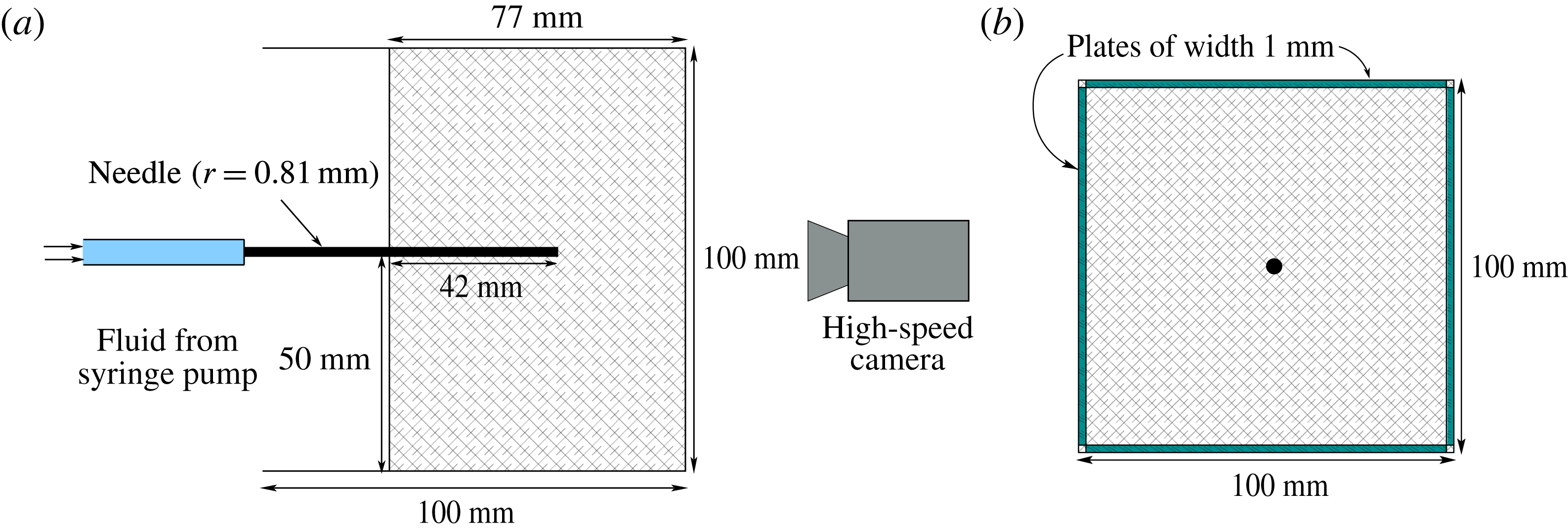
mm was set around an injection needle of radius 0.81 mm, as shown in figure 2. The gel matrix was sufficiently large that the free surface and boundaries had a negligible effect on the stress state near the injection point at the bottom of the needle. The fracturing fluid was pumped at a constant volumetric rate using a syringe pump (WPI AL6000).
In order for the fracture to propagate radially and perpendicularly to the injection needle, we must orientate the needle parallel to the minimum confining stress, as the fracture will propagate perpendicular to this direction. This is due to the fact that the radial crack is a tensile fracture (mode I) and opens in the direction of least resistance. To achieve this, we inserted four rectangular plates of width 1 mm parallel to the needle, on each side of the gel, as shown in figure 2(b). A high-speed camera (Dalsa Falcon 2 4MP) was used to capture the fracture growth. The incompressible Newtonian fracturing fluids used included water, glycerin, silicone and golden syrup, with viscosities in the range
 $\unicode[STIX]{x1D707}\sim 10^{-3}{-}10^{1}~\text{Pa}~\text{s}$
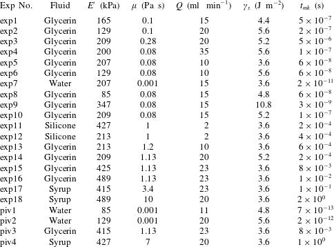
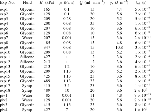
. A list of the experiments and their physical parameters is given in table 2, along with the corresponding characteristic time scales.
Schematic diagrams of the experimental set-up. (a) Elevation view and (b) plan view.

Experiments conducted with particular values of the physical parameters.
The propagation of these fluid fractures was clearly observed due to the transparent nature of the gels. The radial fracture profile was found by dyeing the fluid so that it could be easily distinguished from the surrounding medium. The radius measurements at each time step were then taken from light intensity values. We constructed 20 lines with equally spaced angles between 0 and
 $2\unicode[STIX]{x03C0}$
radians, which radiated from the injection source, and the average of these was chosen as the radius. Digiflow software was used extensively in processing the videos and taking measurements (Dalziel Reference Dalziel2006). The resolution we were able to achieve with these measurements was 1 pixel
 ${\approx}0.04$
mm.
The experimental errors were calculated by estimating uncertainties in the physical parameters of the hydrogel Young’s modulus
 $E$
(
 $\pm 10\,\%$
) and fracture energy
 $\unicode[STIX]{x1D6FE}_{s}$
(
 $\pm 10\,\%$
), experimental uncertainties in the injection rate
 $Q$
(
 $\pm 10\,\%$
) and viscosity
 $\unicode[STIX]{x1D707}$
(
 $\pm 10\,\%$
) of the injected fluid, and measurement errors in the time
 $t$
(
 $\pm 0.2$
s) and radius
 $R$
(
 $\pm 0.5$
mm).
4.2 Aperture measurement
A dye attenuation method was used to measure the fracture aperture. This is a process where the absorption of light is used to relate to aperture measurements (Bunger Reference Bunger2006). A red LED light sheet with a diffuser was used as background lighting to provide a uniform monochromatic light source. The injected fluid was dyed with methylene blue, which strongly absorbs at the wavelength of the red light source. The absorption of this background light is then directly related to the amount of fluid through which it passes.
4.2.1 Calibration
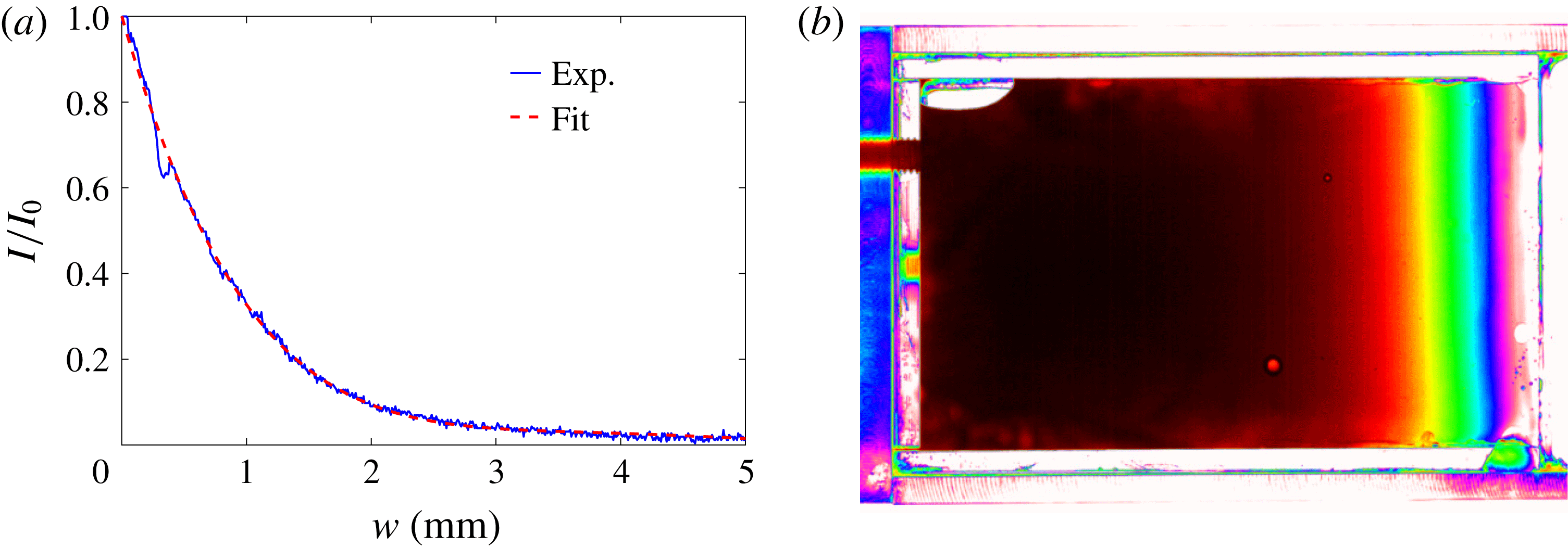
Before the fracture aperture was measured, a calibration experiment was conducted. This experiment involved constructing a glass wedge with a linearly increasing aperture from 0 to 8 mm. This wedge was then filled with dyed fluid (figure 3
b), which was the same fluid as used in the fracturing experiment. The wedge was then placed in our acrylic container (figure 2) and a polyacrylamide gel formed around it, in order to take into account the absorption of light by the gel matrix itself. We denote the intensity of the uniform background light that has travelled through the polyacrylamide gel only by
 $I_{0}$
, and the intensity distribution of light that has passed through the fluid-filled region by
 $I$
. By normalising the fluid-filled light intensity with the background intensity through the gel, the absorption of the light due to the matrix alone can be excluded. We plot this normalisation
 $I/I_{0}$
versus the aperture of the wedge in figure 3(a). A polynomial fit to the calibration data was then determined and used to relate the light intensity data to aperture measurements for fluid-filled fractures, under the assumption that the fracture is symmetric about its midplane.
Due to the particular concentration of dye added to the fluid, measurements above certain thresholds are not very accurate, for example above 2 mm in figure 3(a), where the calibration curve begins to flatten. This sample concentration of
 $0.05~\text{g}~\text{l}^{-1}$
of methylene blue was chosen so that the crack tip profile could be accurately determined.
(a) The normalised light intensity
 $I/I_{0}$
versus the corresponding aperture of the fluid-filled region for a given dye concentration. (b) Experimental image of a calibration using glycerin.

4.3 Particle image velocimetry
In order to capture and explore the fluid flow within the fracture, we used the optical method of PIV. This flow visualisation technique allows instantaneous velocity measurements to be obtained. We created a 10 mm thick light sheet in the plane of fracture growth within the hydrogel, using two arc lamps that penetrated through slits on either side of the experimental apparatus. The fracturing fluid was then seeded with tracer particles of
 $50~\unicode[STIX]{x03BC}\text{m}$
in diameter, which were large enough to track within the fracture but had a negligible influence on the flow itself. When the fracture began to propagate, the fracturing fluid with entrained particles was illuminated so that they were visible relative to the ambient. The two-dimensional velocity data of the fluid in the plane of fracture propagation were then determined by capturing images at 50 fps.
5 Results
In this section, we present the results of experiments in which we explore the radial fracture growth and aperture scalings, outlined in table 1, for both the toughness- and the viscosity-dominated regimes. The crack tip behaviour in each of these regimes is displayed and shown to obey their respective asymptotic solutions, (2.41) and (2.42). Finally, the flow within the fluid-driven fractures is investigated with the use of PIV measurements.
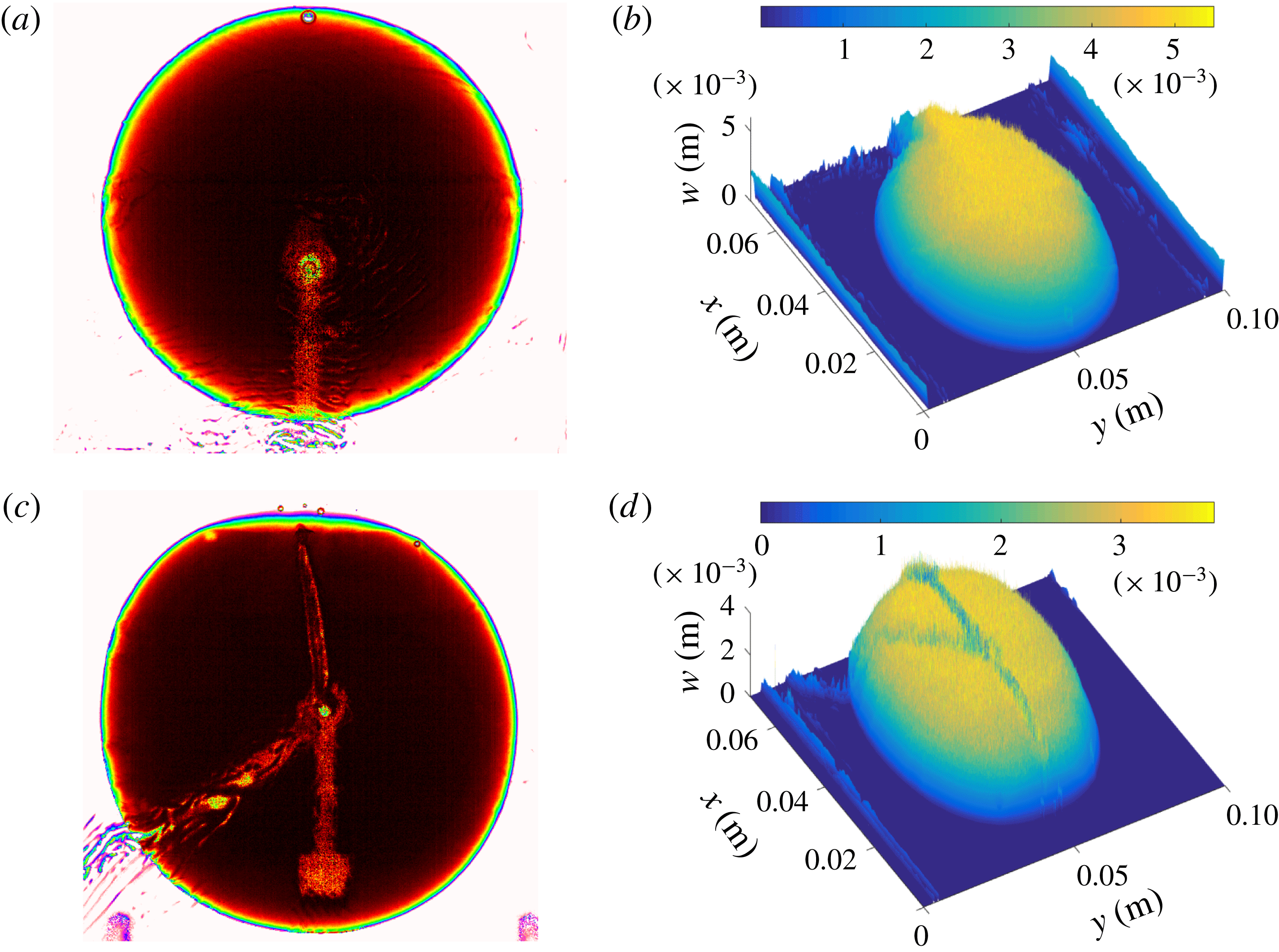
Experimental radial and aperture profiles of sample experiments: (a,b) exp8 (
 $t\approx 39.4$
s); (c,d) exp15 (
 $t\approx 40.6$
s).

5.1 Radial crack growth
Once fluid is injected at a constant flux, a fracture propagates radially outwards from the source, with no observable lag between the fluid-filled region and the crack tip. We can see two examples of this type of fracture in figure 4. Initially, there is a small fast fracture burst when the crack is first formed, due to the release of elastic energy stored in the matrix. After this initial crack is created, the fracture then propagates in the appropriate regime. Generally, toughness-dominated fractures were observed to propagate with slightly more asymmetry than in the viscosity limiting regime. This was mainly due to small heterogeneities in the gel matrix, which play a much larger role when bond-breaking is the dominant energy dissipation mechanism. This behaviour can be seen in figure 4(a,c), where the experiment further into the toughness-dominated regime (exp8) is more asymmetric around the injection centre. The ridges seen in figure 4 are due to the injection tube and the apparatus used to hold the injection needle in place.
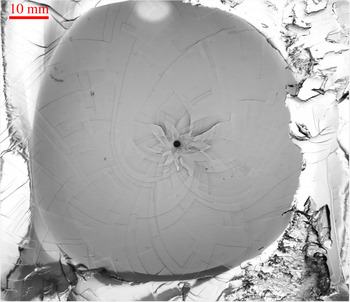
Once the fracturing process was complete, we examined the fracture surface created. This was done by peeling open the gel along the plane of fracture. The fracture pattern created showed evidence of step lines, which can be seen for a typical experiment in figure 5. These patterns have been found in other configurations (Tanaka et al. Reference Tanaka, Fukao, Miyamoto, Nakazawa and Sekimoto1996; Tanaka, Fukao & Miyamoto Reference Tanaka, Fukao and Miyamoto2000), and we have discussed these phenomena extensively elsewhere (O’Keeffe & Linden Reference O’Keeffe and Linden2017).
A typical fracture surface post experiment exhibiting spiral patterns (exp9).

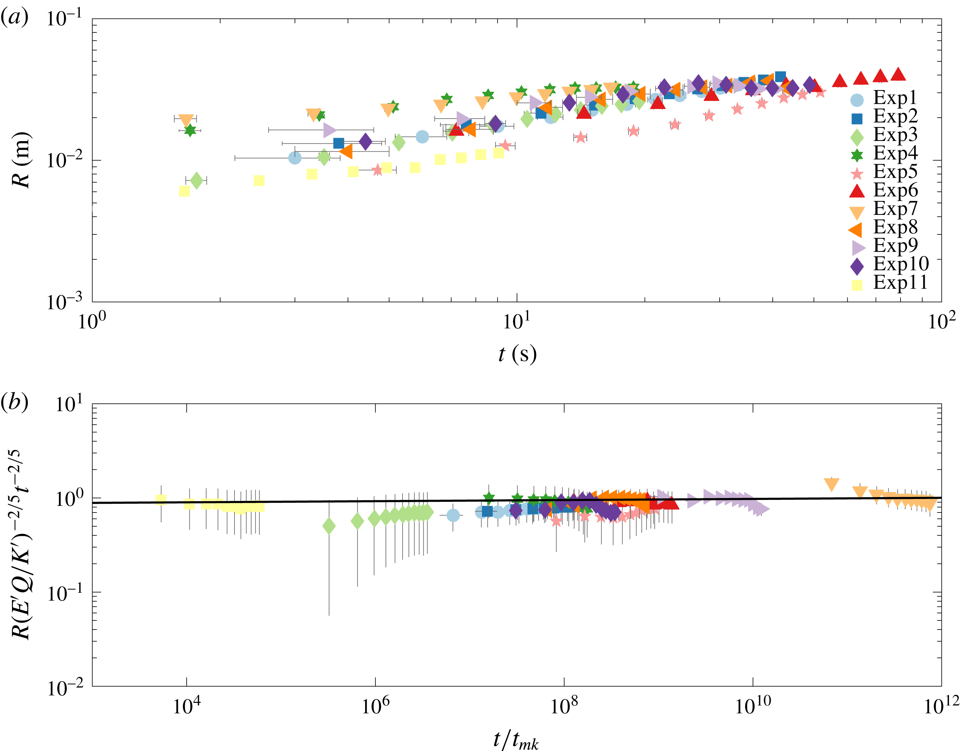
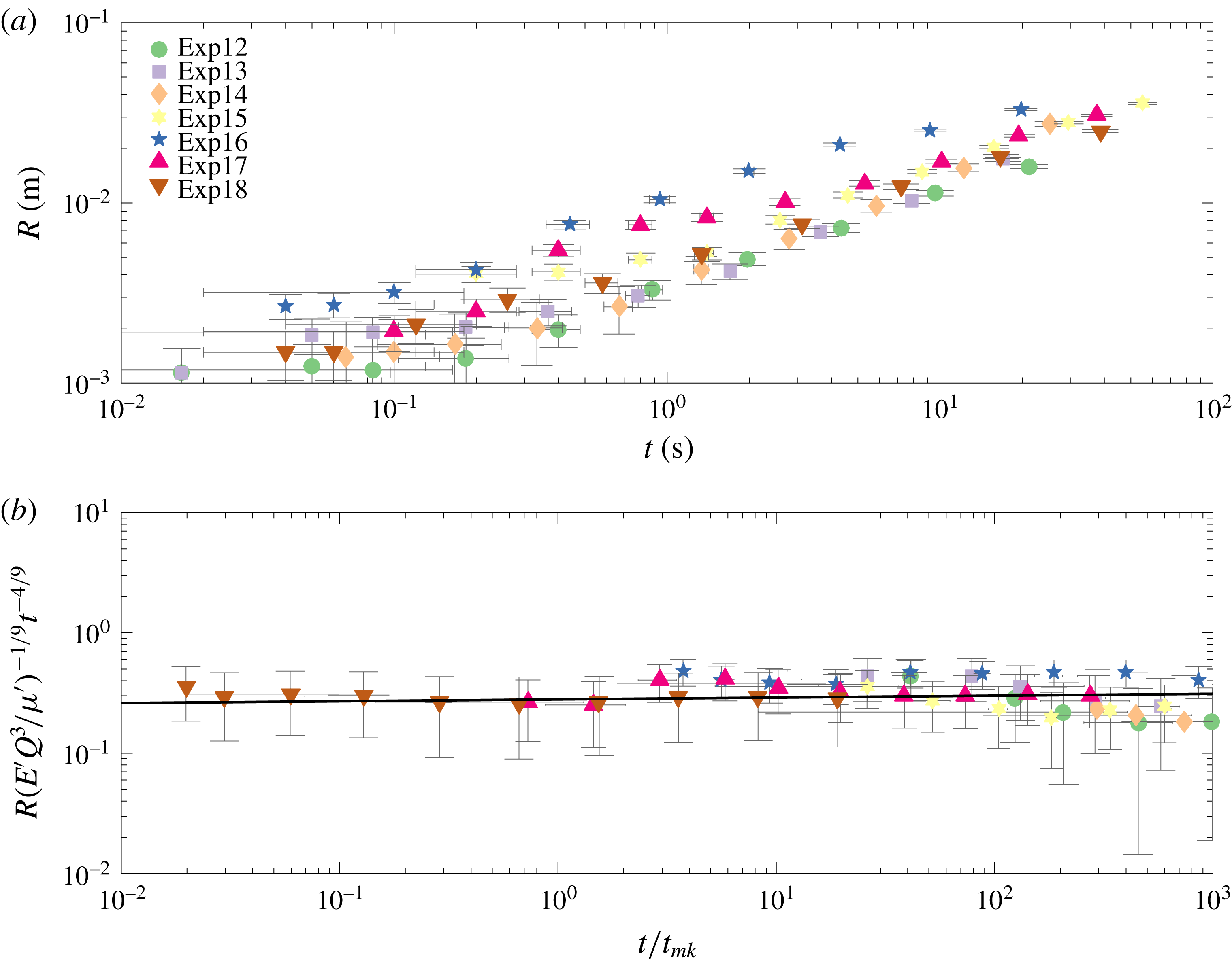
(a) The growing crack radius
 $R$
versus time for a number of experiments with varying injection rate
 $Q$
, viscosity
 $\unicode[STIX]{x1D707}$
and elastic modulus
 $E$
. (b) The toughness rescaling
 $R_{k}(t)$
of crack dependence versus rescaled time
 $t/t_{mk}$
.

(a) The growing crack radius
 $R$
versus time for a number of experiments with varying injection rate
 $Q$
, viscosity
 $\unicode[STIX]{x1D707}$
and elastic modulus
 $E$
. (b) The viscosity rescaling
 $R_{m}(t)$
of crack dependence versus rescaled time
 $t/t_{mk}$
.

In figure 6(a), we plot the radial extent versus time for experiments in the toughness regime i.e. where
 $t\gg t_{mk}$
. These raw data allude to a linear progression on the log–log scale for late times. By rescaling the radius using (2.31) and time with the characteristic time scale (2.37), we produce figure 6(b). We observe that this scaling collapses all of the experimental curves onto a horizontal line which obeys the
 $t^{2/5}$
power law, as expected for late times. The best fit line has a prefactor
 $k=0.86\pm 0.18$
and exponent
 $\unicode[STIX]{x1D6FC}_{k}=0.4\pm 0.04$
, where
 $$\begin{eqnarray}R_{k}(t)=k\left(\frac{{E^{\prime }}^{2}Q^{2}}{{K^{\prime }}^{2}}\right)^{1/5}t^{\unicode[STIX]{x1D6FC}_{k}}.\end{eqnarray}$$
This agrees well with the theoretical prefactor, which has a value of 0.85 from Savitski & Detournay (Reference Savitski and Detournay2002). On accounting for the different constants used in the scaling of Lai et al. (Reference Lai, Zheng, Dressaire and Stone2016), the prefactor in that study would correspond to a value of
 $k=0.56$
.
Figure 7(a) plots the crack radius
 $R$
versus time for experiments in the viscous regime, in which
 $t\lesssim t_{mk}$
. Again, the raw data follow a power law, and, using the radial viscosity-dominated scaling as in table 1, we find that the data collapse onto the same horizontal line (figure 7
b). The best fit line has a prefactor
 $m=0.28\pm 0.15$
and exponent
 $\unicode[STIX]{x1D6FC}_{m}=0.46\pm 0.04$
, where
 $$\begin{eqnarray}R_{m}(t)=m\left(\frac{E^{\prime }Q^{3}}{\unicode[STIX]{x1D707}^{\prime }}\right)^{1/9}t^{\unicode[STIX]{x1D6FC}_{m}}.\end{eqnarray}$$
The prefactor
 $m$
differs significantly in the viscous regime from the theoretical value of 0.7. To account for this discrepancy we examined some possibilities.
(i) There may have been storage of fracturing fluid in the initial stages of the experiment, leading to a different value of
$Q$
from the expected one. This was explored using PIV measurements from § 5.4. The resulting flux estimates from the velocity data match the syringe pump values to within approximately 10 %, suggesting that storage effects were negligible and
$Q$
was accurately reported.(ii) The parameter values were not as prescribed. However, we believe that the experimental parameters are well characterised. Young’s modulus
$E$
was calculated from two different methods, compression tests and spherical indentation, and the fluid viscosity
$\unicode[STIX]{x1D707}$
was measured using a u-tube viscometer before every experiment. In order for our experimental viscous prefactor to match the theoretical value of 0.7, the ratio of
$E^{\prime }Q^{3}/\unicode[STIX]{x1D707}$
would have to be significantly different as it is raised to a power of
$1/9$
.(iii) The viscosity regime does not start at time
$t=0$
. This could be due to the initial elastic response of the hydrogel. However, estimates for the maximum value of this from
$t_{om}=E^{\prime }\unicode[STIX]{x1D707}^{\prime }/\unicode[STIX]{x1D70E}_{0}^{3}\approx 0.03$
are not sufficient to explain the difference (Bunger & Detournay Reference Bunger and Detournay2007). We can fit the theoretical prefactor to the data, where time is equal to
$(t-t_{om})$
, to find a suitable
$t_{om}$
after which the viscosity regime propagates. We find that the
$t_{om}$
value is in the range
${\approx}5{-}25$
s, which seems to be an implausibly long time.





This analysis suggests that there may be some unidentified physical mechanisms that were unaccounted for in the modelling, and that are responsible for this experimental underprediction. A similar discrepancy can be found in the study by Lai et al. (Reference Lai, Zheng, Dressaire, Wexler and Stone2015), where their scaling argument has an extra constant
 $(1/32\unicode[STIX]{x03C0}^{3})^{1/9}$
when compared with (5.2). The rescaled data in that study have a prefactor of 0.62, which would correspond to a value of
 $m=0.29$
here using (5.2). Therefore, both their and our independent experimental studies exhibit similar underpredictions.
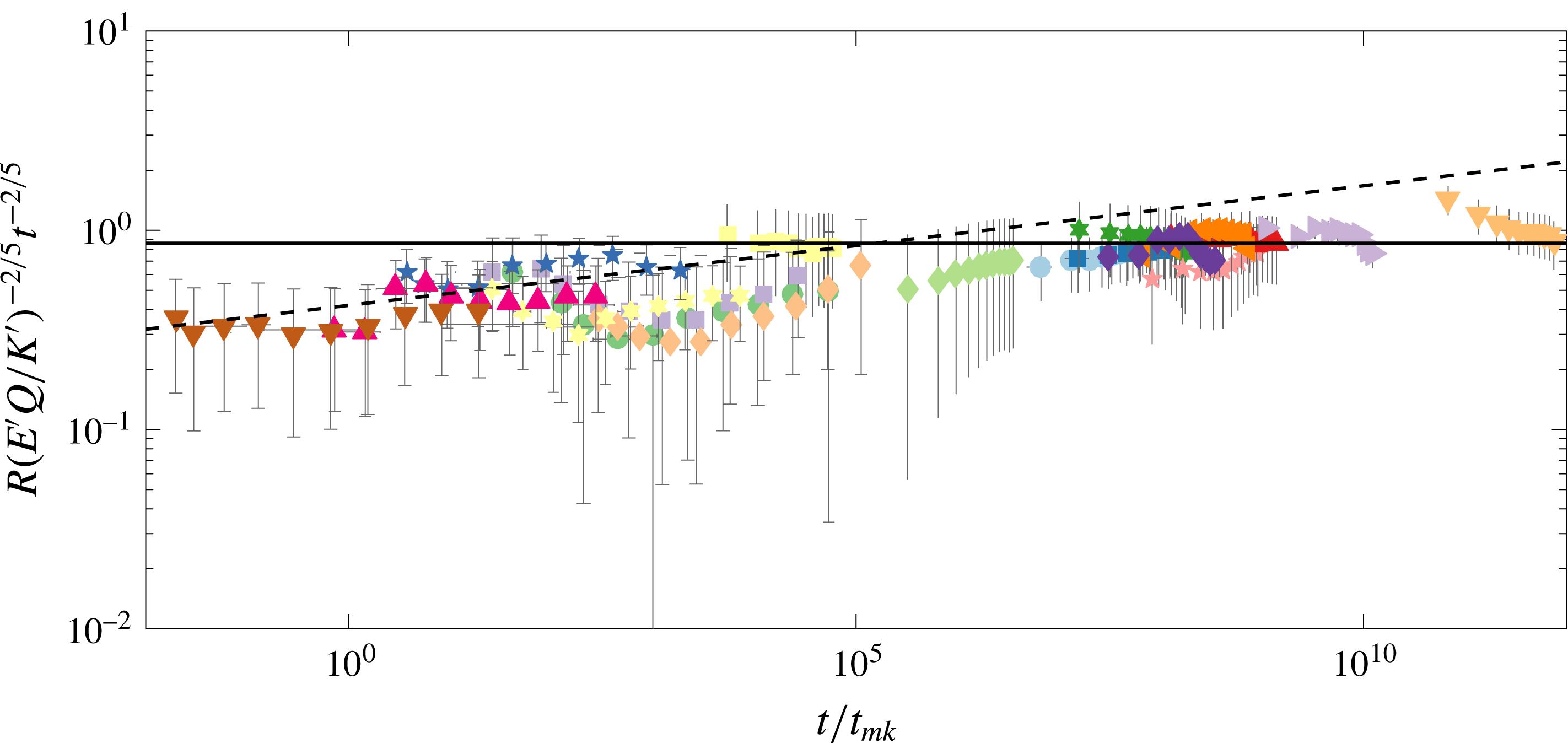
All experiments scaled using the radial toughness-dominated power law (2.31).

To distinguish between regimes, we plot all experiments scaled with the toughness-dominated radial power law (2.31) in figure 8. The dashed line is fitted to experiments where
 $t/t_{mk}\lesssim 10^{2}$
, and this has a prefactor of
 $0.42\pm 0.13$
and exponent of
 $0.46\pm 0.04$
. Likewise, the black line is fitted to experiments where
 $t/t_{mk}\gtrsim 10^{2}$
, and this has a prefactor and exponent as before of
 $k=0.86\pm 0.18$
and
 $\unicode[STIX]{x1D6FC}_{k}=0.4\pm 0.04$
. This large difference in the prefactors and exponents between the two groups of experiments shows that it is possible to distinguish between the two different regimes. One particular experiment, exp16, is known to transition from a viscous- to a toughness-dominated regime, and will be discussed in detail in § 5.3. The raw data for these experimental measurements are contained in the supplementary material, available at https://doi.org/10.1017/jfm.2018.203.
5.2 Crack aperture
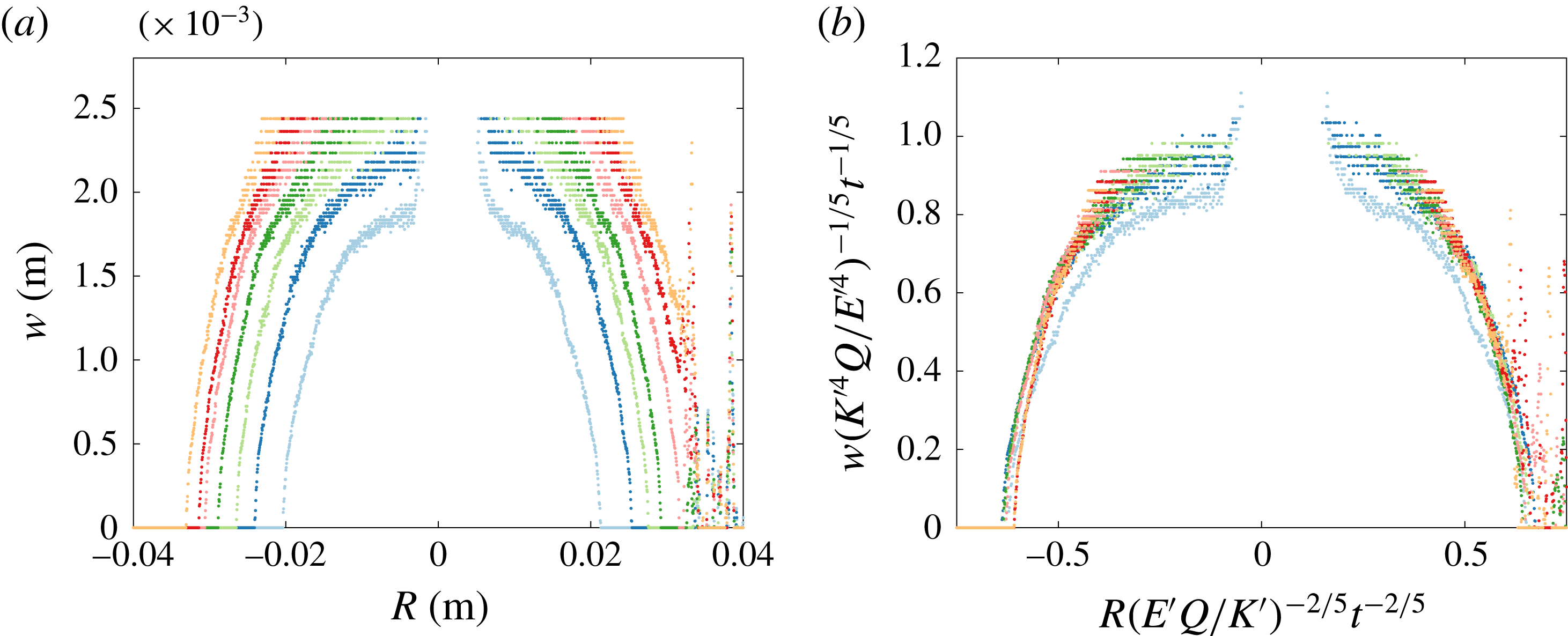
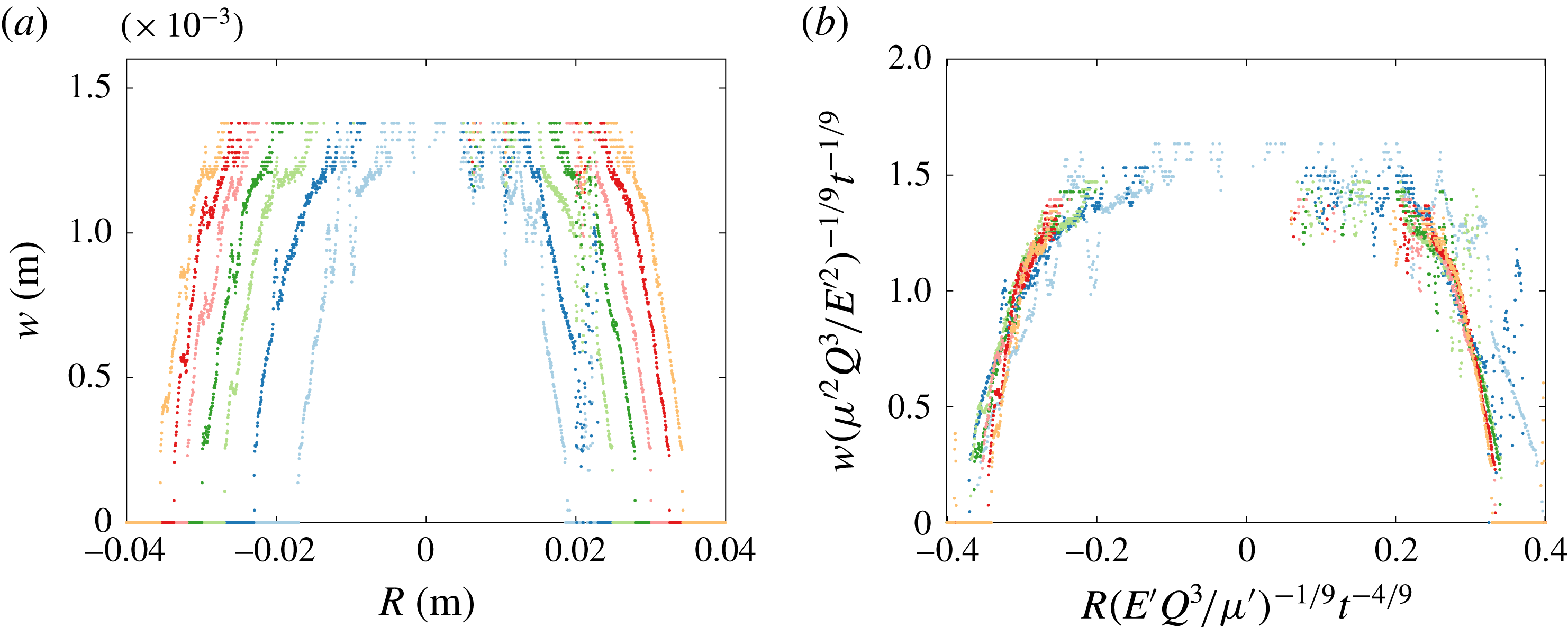
The crack aperture measurements obtained from dye attenuation provide us with the full crack profile. In figures 9 and 10, we plot the cross-section, which intersects the injection needle so we can properly analyse the crack aperture scalings. The anomalous points observed in the data for both experiments, which occur around
 $R=0$
, are due to the presence of the injection needle blocking measurements at this point.
In figure 9(a), the width versus radius is plotted for a fracture in the toughness-dominated regime. Each curve corresponds to the crack aperture at a certain time, with the curves at the outer edges corresponding to the later times. Figure 9(b) shows that scaling the cross-section data, with the radial and width toughness power laws from table 1, results in collapse of the curves.
Results from an experiment near the viscosity regime are shown in figure 10. Once again, the curves collapse under the appropriate scalings onto a single curve, as seen in figure 10(b), thus behaving in the expected way as outlined in table 1. Although figures 9 and 10 only correspond to two particular experiments (exp9 and exp15), this behaviour is reproduced by other experiments (not shown). The scaled data produce a very well-behaved radius collapse, while the error near the centre of the fracture is related to the tuning of the calibration to capture the tip behaviour.
(a) The crack aperture profile of a cross-section, intersecting the injection needle, of the radial fracture for experiment exp9 (table 2). Each set of data points corresponds to the crack aperture at a certain time, with time evolving outwards in increments of
 $\unicode[STIX]{x0394}t=4$
s from the crack centre for each curve. (b) The rescaled fracture aperture profile using the toughness-dominated radial and width power-law scalings from table 1.

(a) The crack aperture profile of a cross-section, intersecting the injection needle, of the radial fracture for experiment exp16 (table 2), with
 $\unicode[STIX]{x0394}t=4$
s. (b) The rescaled fracture aperture profile using the viscosity-dominated radial and width power-law scalings from table 1.

5.3 Crack tip behaviour
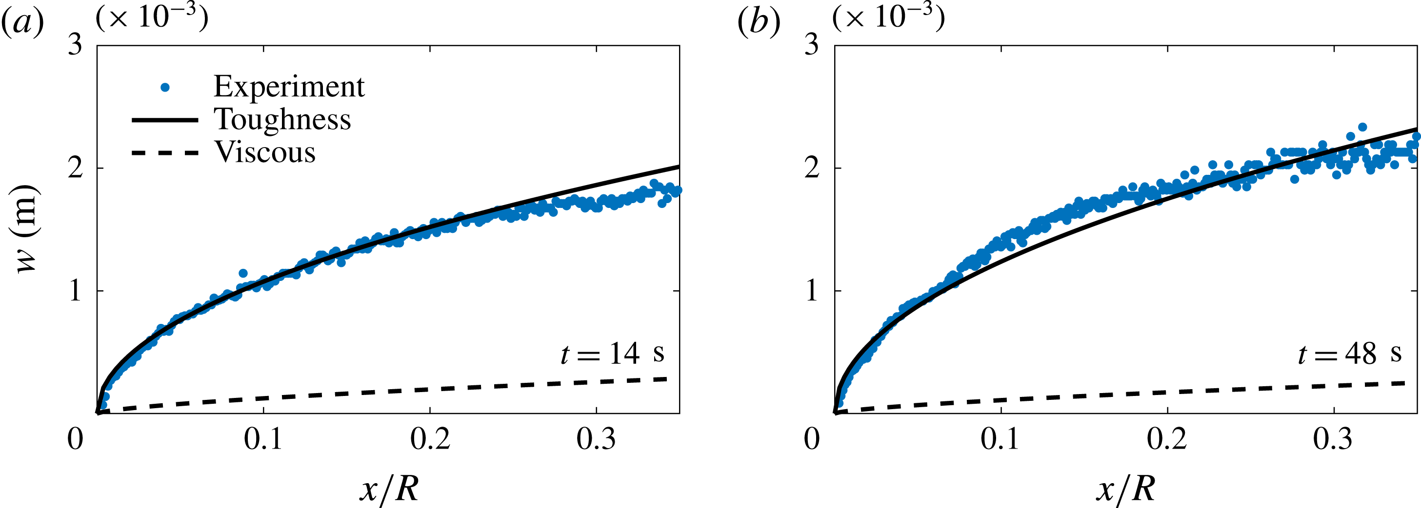
These aperture measurements also allow us to explore the tip behaviour of these fractures. This method provides an extra validation of the toughness and viscous regimes while also allowing us to observe the transition between regimes. Figure 11 shows the crack tip opening profile for a fracture propagating in the toughness-dominated regime compared with the asymptotic forms for the toughness and viscous regimes, (2.41) and (2.42) respectively. It is clearly seen that the LEFM asymptotic behaviour in (2.41) is observed for different times throughout the experiment.
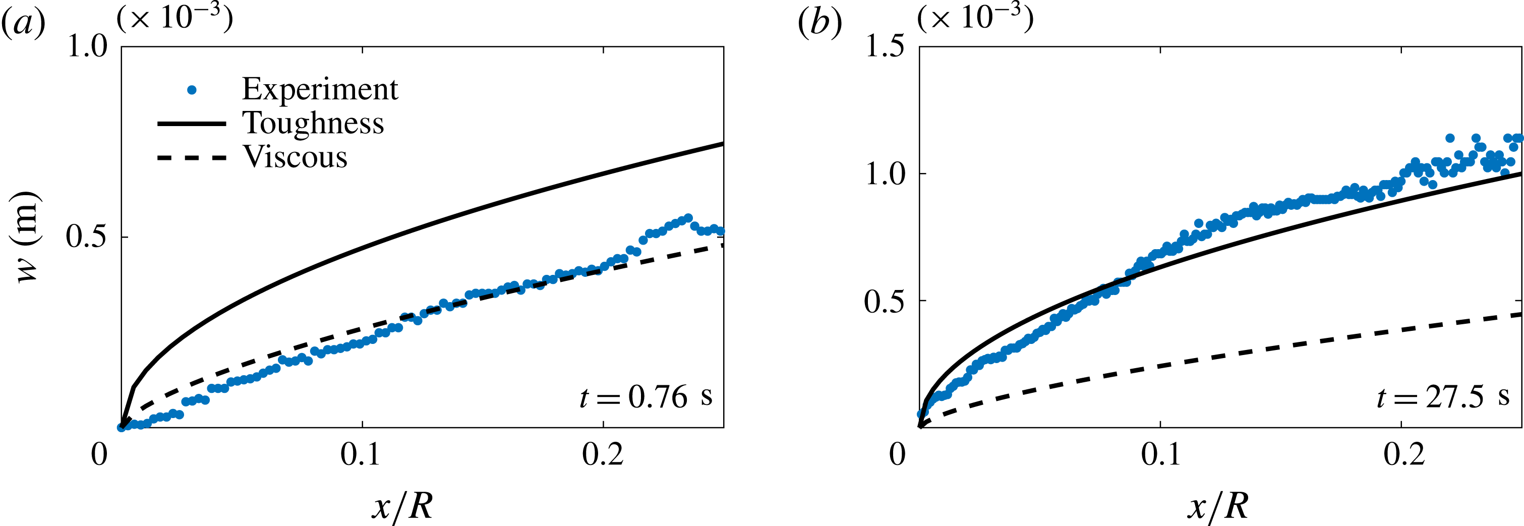
Figure 12 shows the transition from a viscous- to a toughness-dominated fracture. Figure 12(a) shows that the tip region is governed by the viscous intermediate asymptote (2.42) in the limiting case of the viscosity-dominated regime at
 $t=0.76$
s. As the fracture evolves, the crack tip then transitions to the toughness-dominated regime at later times. Figure 12(b) shows the crack shape in this regime.
The crack tip region for a toughness-dominated fracture (exp10) that follows the LEFM toughness asymptote (2.41) denoted by the solid line for (a)
 $t/t_{mk}=1.4\times 10^{8}$
and (b)
 $t/t_{mk}=4.8\times 10^{8}$
.




5.4 Fracture fluid flow
In modelling the radial fracture problem, we have assumed (see (2.6)) that lubrication theory adequately captures the physical mechanisms of the flow, meaning that the flow is laminar and radial in nature. The appropriate Reynolds number for the lubrication fluid flow in the fracture is defined in (2.5).
If we first consider an example of a fracture near the viscosity-dominated regime (piv3, table 2), where
 $Q\approx 23~\text{ml}~\text{min}^{-1}$
,
 $\unicode[STIX]{x1D707}\approx 1130$
mPa s,
 $E\approx 311$
kPa,
 $\unicode[STIX]{x1D6FE}_{s}\approx 3.6~\text{J}~\text{m}^{-2}$
,
 $\unicode[STIX]{x1D70C}\approx 1.26~\text{g}~\text{cm}^{-3}$
,
 $w\approx 1.7$
mm and
 $R\approx 25$
mm, then
 $Re_{m}\approx 1.9\times 10^{-4}$
(
 $t_{mk}\sim 0.008$
). In a toughness limiting regime (piv2, table 2), where
 $\unicode[STIX]{x1D707}\approx 1$
mPa s,
 $E=97$
kPa,
 $Q=20~\text{ml}~\text{min}^{-1}$
,
 $\unicode[STIX]{x1D6FE}_{s}=5.6~\text{J}~\text{m}^{-2}$
,
 $\unicode[STIX]{x1D70C}\approx 1~\text{g}~\text{cm}^{-3}$
,
 $w\approx 2$
mm and
 $R\approx 25$
mm, then
 $Re_{k}\approx 1.7\times 10^{-1}$
(
 $t_{mk}\sim 10^{-12}$
). This approximation suggests that the range of Reynolds numbers involved is sufficiently small that inertial effects can be neglected.
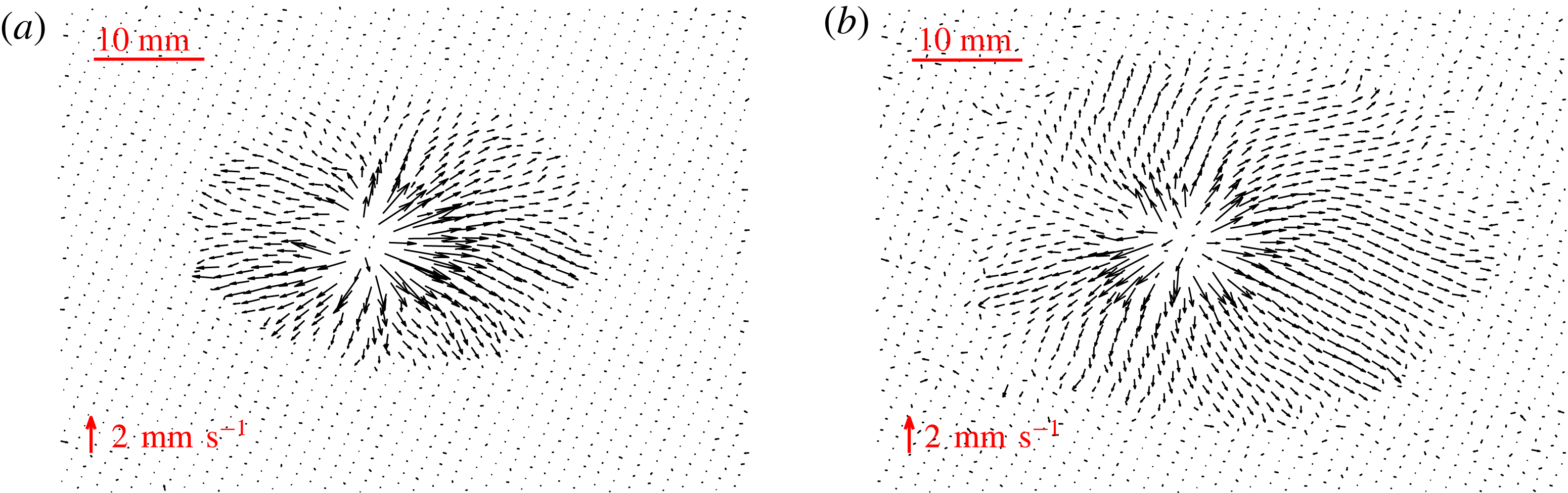
Velocity fields for a fracture in the viscosity regime (piv4) for (a)
 $t/t_{mk}\sim 10$
and (b)
 $t/t_{mk}\sim 20$
.

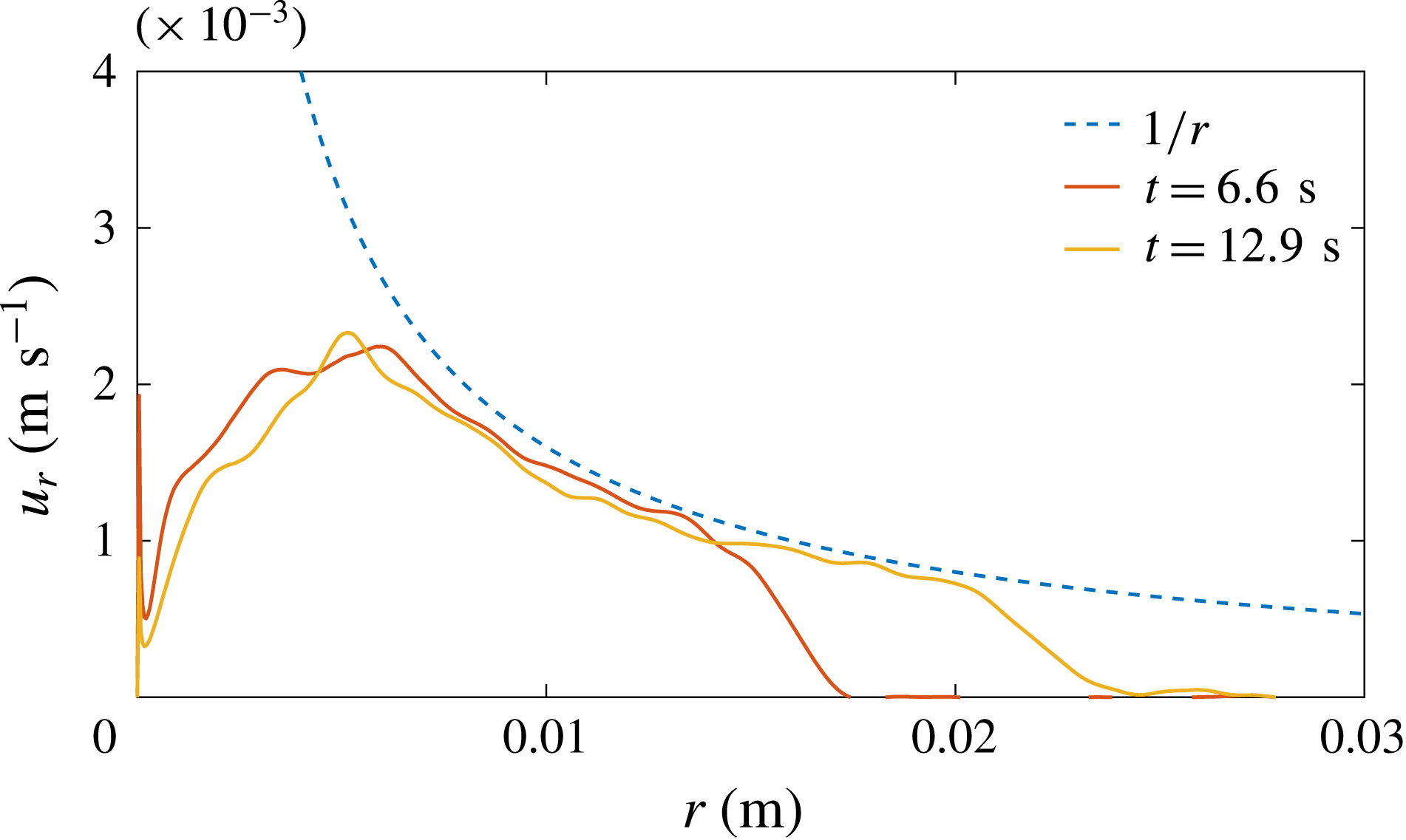
Azimuthal velocity average of fluid versus distance from the source
 $r$
.

Examples of the velocity field in the viscosity regime (piv4, table 2) obtained from the PIV measurements are shown in figure 13. The velocity fields exhibit laminar radial flow emanating from the injection needle source in the centre of the fracture. The magnitude of the velocity vectors diminishes with distance from the source, which is consistent with a constant volume flux spreading radially outwards, where velocity decays like
 $r^{-1}$
. This is observed in figure 14, where the azimuthal by-averaged radial velocity is plotted versus distance from the source for the two times seen in figure 13. This type of behaviour is expected and was assumed in our mathematical formulation, which used lubrication theory to predict the flow.
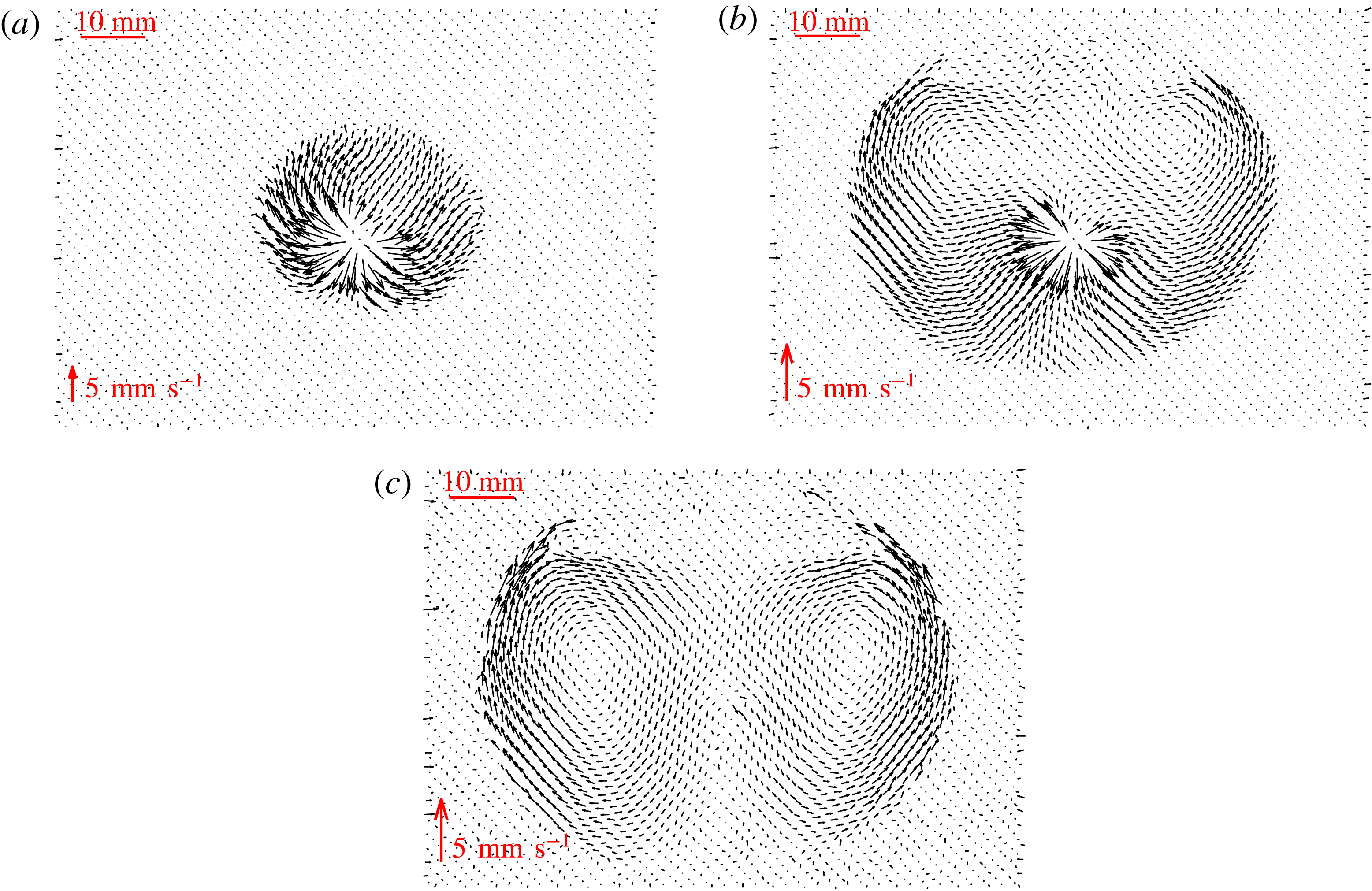
The velocity fields in an experiment that transitions from a viscosity- to a toughness-dominated fracture regime (piv3, table 2), are shown in figure 15. In figure 15(a), the velocity field at early times when
 $t/t_{mk}\sim 10^{2}$
is similar to that observed in the viscosity regime, as anticipated. However, at later times in the experiment (figure 15
b,c) when the fracture has transitioned fully into the toughness regime, the fracturing fluid noticeably circulates around the fracture once it has reached the tip. Two small circulations form at the top of the fracture and grow in size as the crack propagates radially, until they finally encompass the whole fluid-filled fracture.
Average velocity fields at different stages for a fracture transitioning between regimes (piv3) for (a)
 $t/t_{mk}\sim 5\times 10^{2}$
, (b)
 $t/t_{mk}\sim 5\times 10^{3}$
and (c)
 $t/t_{mk}\sim 1\times 10^{4}$
.

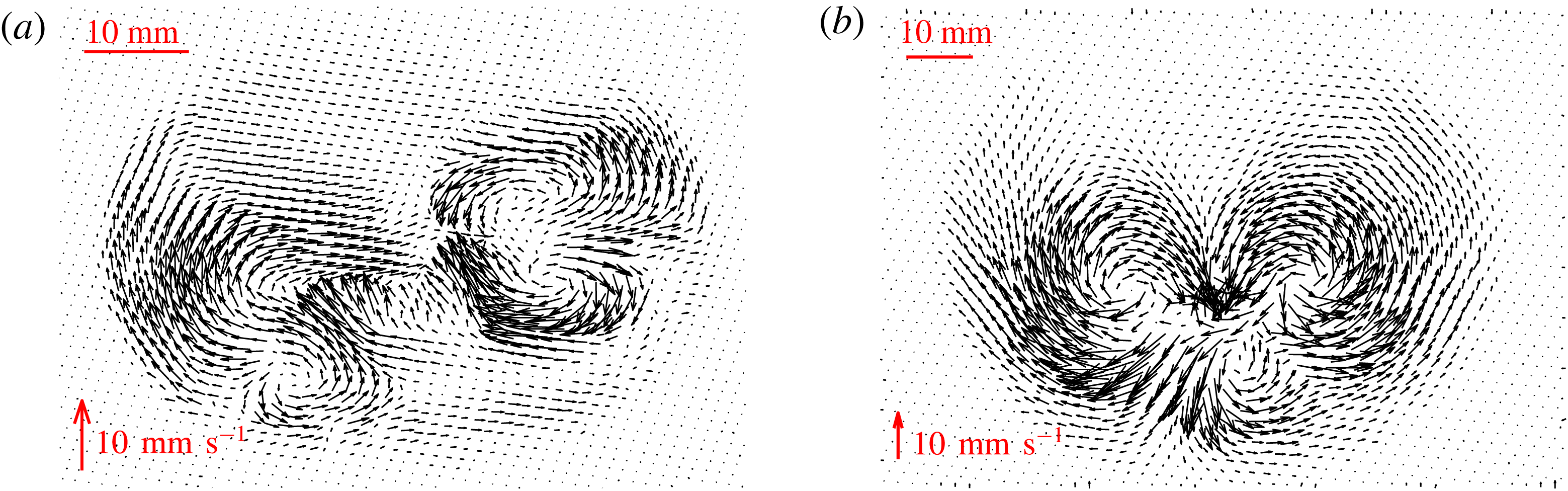
For experiments that are toughness-dominated at all times, the flow within the fracture can be very disordered. Figure 16 shows the average velocity fields for two such experiments at late times. Similarly to the late-time behaviour of the transitioning fracture, the structure of the flow appears to be split into circulation cells within the fracture, which are quite different from the assumed flow field under lubrication theory. The number of cells that formed varied between experiments. So far, we have observed a variation between 1 and 4 for the number of cells present in a single fracture.
This behaviour is thought to be due to the extent of the departure of the crack shape from a perfect circle around the injection needle. Initially, a small asymmetry in the fracture shape usually occurs due to the experimental conditions, such as small heterogeneities in the gel. The injected fluid is then drawn into the tip of the quasistatically propagating fracture, which is not propagating at exactly the same rate at every point of the fracture. Some preferential direction will be established at each time step of propagation. This area will attract more fluid within the fracture. Then, once this preferential direction has changed, the fluid present will circulate around to the more dominant area of growth. This type of behaviour can be seen in figure 15, where the fracture initially grows preferentially upwards and then the flow begins to circulate around when more fracturing occurs downwards at later times.
Average velocity fields at late times for fractures in the toughness regime for (a)
 $t/t_{mk}\sim 10^{12}$
(piv1) and (b)
 $t/t_{mk}\sim 10^{11}$
(piv2).

6 Conclusions
This paper describes the properties of fluid-driven fractures in an elastic medium. We first reviewed the existing theoretical framework for a fluid-driven penny-shaped crack. This literature provided scaling relationships of fracture radius, aperture and crack tip shape dependent on the dominant energy dissipation mechanism, viscosity or material toughness. These relationships were then verified experimentally in brittle hydrogels, with transitions between the two regimes also observed. It can be difficult to distinguish between regimes due to the similarity of the respective power laws describing the growth of the fracture radius with time. This motivated three dynamic measurements, radius, aperture and velocity, to identify the presence of limiting regimes and the possibility of experimentally observing the transition. The toughness regime measurements for radius growth provide good agreement between experimental and theoretical prefactor values. However, the discrepancy observed between the prefactors in the viscous regime is significant, suggesting that some unknown physical mechanism might be unaccounted for. It is extremely important in industrial applications of hydraulic fracturing that the regime of propagation is known. The injection time scales for these operations can sometimes be several days. Therefore, even though the power-law dependence for radial growth is similar, over large time scales, fractures will propagate significantly further in the viscosity regime compared with toughness-dominated cracks.
Finally, PIV analysis of fluid within these fractures revealed that two distinct types of flow are also present. In the viscosity limiting case, the fluid travels radially outwards from the source to the tip, as expected. However, in the toughness limiting case, where the quasistatic propagation of the crack is not dependent on the flow, the fracturing fluid travels in a more complex manner, circulating within the crack. This type of flow will have a significant effect on the transport of proppants within fractures, and ultimately on the success of a hydraulic fracturing operation. The flow pattern may inhibit the ability of the proppants to travel to desired locations so that fractures are propped open and gas extracted.
Acknowledgements
We would like to thank J. L. Partridge, D. Page-Croft and the technicians in the G. K. Batchelor Laboratory for their help in setting up the experiment. We also acknowledge helpful discussions with J. Neufeld and C. Rennie (industrial supervisor). This work was funded with the support of an iCASE award from the EPSRC and BP (grant no. EP/L505389/1).
Supplementary material
Supplementary material is available at https://doi.org/10.1017/jfm.2018.203.