1. Introduction
We present a parallel particle-in-cell (PIC) code for the numerical simulation of ultrarelativistic charged beams in supercolliders based on the three-dimensional (3-D) set of Maxwell’s equations for the electromagnetic fields, and the Vlasov equation for the distribution function of the beam particles. The code takes into account high relativistic factor values and highly nonlinear charge density distribution.
The electric field of a relativistic charged particle can be described in the laboratory coordinate system as
 $$\begin{eqnarray}\boldsymbol{E}=\frac{1}{{\it\gamma}^{2}}\frac{1}{(1-{\it\beta}^{2}\sin ^{2}{\it\theta})^{3/2}}\frac{q\boldsymbol{R}}{R^{3}},\end{eqnarray}$$
where
 $\boldsymbol{R}$
is the radius-vector from the particle to the observation point,
 ${\it\theta}$
is the angle between the motion direction and the radius-vector
 $\boldsymbol{R}$
,
 ${\it\beta}=|\boldsymbol{v}|/c$
,
 ${\it\gamma}=1/\sqrt{1-|\boldsymbol{v}|^{2}/c^{2}}$
is the relativistic factor and
 $\boldsymbol{v}$
is the particle velocity. In comparison with the case of non-relativistic motion, the electric field of the particle arises
 ${\it\gamma}$
times in the transversal direction and decreases
 ${\it\gamma}^{2}$
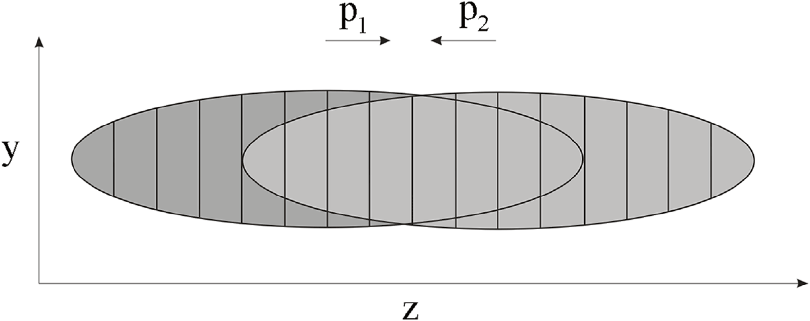
times in the longitudinal direction. The standard algorithms for the numerical simulation of beam–beam effects are based on this fact. The colliding beams are divided into thin macroparticle slices along the axis of the collective motion (figure 1), the field of each slice is considered transverse. Two slices of the colliding beams interact when their longitudinal coordinates coincide: the particles of one beam receive a kick of the transverse 2-D fields of the oncoming beam, changing their motion (Anderson Reference Anderson1998), then the beams switch roles. Usually, the transversal field is calculated using the Basetti–Erskine equations (Basetti & Erskine Reference Basetti and Erskine1980) or the derivative of the 2-D potential. The slices are cut into cells, the Poisson equation with boundary conditions or the Green function can be used to obtain the potential (Schulte Reference Schulte1996; Qiang, Furman & Ryne Reference Qiang, Furman and Ryne2004).
The colliding beams divided into macroparticle slices.

This quasi-3-D approach is used for studying the problem of ‘strong–strong’ interactions. However, reduction to the 2-D problem, where the longitudinal motion is simulated by ‘rearranging’ the slices, accounts for the longitudinal effects, which are of particular importance for colliding beams with super-high densities. In the case of abrupt beam deformation, the usual slice number (5–50) may be unacceptably small. The electrostatic approach does not describe correctly the wave propagation in the transversal direction in the case of dramatically disrupting beams and the energy spreading may interrupt the physical experiment. Moreover, simulations using this model become complicated when the beams cross at an angle (Hirata Reference Hirata1995).
In the fully 3-D consideration, the relativistic factor does not facilitate calculations in the same way. The main difficulty of 3-D modelling is due to the high relativistic factors of the particles: the dependence on
 ${\it\gamma}$
in ultrarelativistic cases (
 ${\it\gamma}\sim 10^{3}{-}10^{5}$
) provides high gradients and high errors in the beam fields. In the case of open boundary conditions, the usual beam field computation is connected with implementation of a fine grid in the longitudinal direction and domain extension in the transversal direction and requires very high computer resources to achieve sufficient accuracy. The summation of the field contributions of
 $N_{d}$
beam density nodes for a spatial grid with, for example,
 $N^{3}=100^{3}$
nodes and
 ${\it\gamma}\sim 10^{3}$
requires
 ${\it\gamma}^{3}N^{3}N_{d}=10^{15}N_{d}$
operations and renders the problem unsolvable with standard methods, even with the help of supercomputers.
Our 3-D algorithm obviates the above difficulties by using the Vlasov–Liouville equation for the distribution function of the beam particles, the 3-D set of Maxwell’s equations and special methods for the calculation of the initial and boundary conditions (Boronina et al.
Reference Boronina, Vshivkov, Levichev, Nikitin and Snytnikov2007; Vshivkov & Boronina Reference Vshivkov and Boronina2012). We solve these equations by using the PIC method (Hockney & Eastwood Reference Hockney and Eastwood1981) and the leap-frog scheme (Langdon & Lasinski Reference Langdon and Lasinski1976). The parallel code is based on domain decomposition along the transversal direction whereby every processor group handles its own part of the subdomain grid and all of the particles of the subdomain. Additionally, we employ particle parallelization: within the group, every processor manages its own portion of particles. This method overcomes the high restrictions on the particle number due to the high nonlinearity of the density distribution and of limited processor memory. For example, for 6 processors and a
 $100\times 102\times 100$
grid, the two central processors contain almost half of the particles, the memory limit is
 $2\times 10^{6}$
particles in a processor, hence,
 $5\times 10^{6}$
particles in the beam, which indicates quite a small particle number in cell for the PIC method. The parallel supercomputer version makes possible beam–beam simulations for supercritical parameters.
2. Mathematical model
We consider motion of colliding electron–positron beams in a rectangular domain
 $[0,L_{x}]\times [0,L_{y}]\times [0,L_{z}]$
. The motion takes place in vacuum in self-consistent electromagnetic fields taking into account the external focusing field. Each beam is defined by its shape, dimensions, coordinates in space and time, particle number and nonlinear density distribution. No radiation effects are considered. The aim is to analyse the particle dynamics dependence on the given beam configuration.
The motion is described with the Vlasov kinetic equation for the distribution function of electrons
 $f_{-}=f_{-}(\boldsymbol{r},\boldsymbol{p},t)$
and positrons
 $f_{+}=f_{+}(\boldsymbol{r},\boldsymbol{p},t)$
:
 $$\begin{eqnarray}\frac{\partial f_{+,-}}{\partial t}+\boldsymbol{v}_{+,-}\frac{\partial f}{\partial \boldsymbol{r}}+\boldsymbol{F}_{+,-}\frac{\partial f}{\partial \boldsymbol{p}}=0,\end{eqnarray}$$
and the 3-D Maxwell’s equations:
 $$\begin{eqnarray}\displaystyle & \displaystyle \text{rot}\,\boldsymbol{E}=-\frac{1}{c}\frac{\partial \boldsymbol{H}}{\partial t} & \displaystyle\end{eqnarray}$$
 $$\begin{eqnarray}\displaystyle & \displaystyle \text{rot}\,\boldsymbol{H}=\frac{4{\rm\pi}}{c}\boldsymbol{j}+\frac{1}{c}\frac{\partial \boldsymbol{E}}{\partial t} & \displaystyle\end{eqnarray}$$
 $$\begin{eqnarray}\displaystyle & \displaystyle \text{div}\,\boldsymbol{E}=4{\rm\pi}(n_{-}e^{-}+n_{+}e^{+}) & \displaystyle\end{eqnarray}$$
 $$\begin{eqnarray}\displaystyle & \displaystyle \text{div}\,\boldsymbol{H}=0, & \displaystyle\end{eqnarray}$$
 $\boldsymbol{p}={\it\gamma}_{+,-}m_{e}\boldsymbol{v}_{+,-}$
and the Lorentz force
 $\boldsymbol{F}_{+,-}=e^{+,-}(\boldsymbol{E}+(\boldsymbol{v}_{+,-}/c)\times \boldsymbol{H})$
.
The charge densities and the currents are the distribution function moments:
 $$\begin{eqnarray}\displaystyle & \displaystyle n_{+}=\int _{V}f_{+}\,\text{d}V, & \displaystyle\end{eqnarray}$$
 $$\begin{eqnarray}\displaystyle & \displaystyle n_{-}=\int _{V}f_{-}\,\text{d}V, & \displaystyle\end{eqnarray}$$
 $$\begin{eqnarray}\displaystyle & \displaystyle \boldsymbol{j}=\int _{V}(\,f_{+}\boldsymbol{v}e-f_{-}\boldsymbol{v}e)\,\text{d}V. & \displaystyle\end{eqnarray}$$
The characteristic equations of the Vlasov kinetic equation coincide with the particle motion equations:
 $$\begin{eqnarray}\displaystyle & \displaystyle \frac{\text{d}\boldsymbol{p}_{+,-}}{\text{d}t}=\boldsymbol{F}_{+,-}, & \displaystyle\end{eqnarray}$$
 $$\begin{eqnarray}\displaystyle & \displaystyle \frac{\text{d}\boldsymbol{r}_{+,-}}{\text{d}t}=\boldsymbol{v}_{+,-}. & \displaystyle\end{eqnarray}$$
All the equations are written in dimensionless variables, the characteristic length
 $L$
of the beam is 1 cm and the characteristic speed
 $v$
of the particles is the speed of light,
 $c=299\,792.458~\text{km}~\text{s}^{-1}$
. We use the PIC method with a PIC form factor and the leap-frog scheme (Langdon & Lasinski Reference Langdon and Lasinski1976; Hockney & Eastwood Reference Hockney and Eastwood1981), where all the components are calculated at the half-step of the time and space grids. In this case, all the derivatives involved in the equations are written with central differences, and this scheme provides second-order accuracy in time and space. For example, we use the following scheme for Maxwell’s equations:
 $$\begin{eqnarray}\displaystyle & \displaystyle \frac{\boldsymbol{H}^{m+1/2}-\boldsymbol{H}^{m-1/2}}{{\it\tau}}=-\text{rot}_{h}\boldsymbol{E}^{m}, & \displaystyle\end{eqnarray}$$
 $$\begin{eqnarray}\displaystyle & \displaystyle \frac{\boldsymbol{E}^{m+1}-\boldsymbol{E}^{m}}{{\it\tau}}=\boldsymbol{j}^{m+1/2}+\text{rot}_{h}\boldsymbol{H}^{m+1/2}. & \displaystyle\end{eqnarray}$$
The second-order scheme for the momentum is the following:
 $$\begin{eqnarray}\frac{\boldsymbol{p}^{m+1/2}-\boldsymbol{p}^{m-1/2}}{{\it\tau}}=q\left(\boldsymbol{E}^{m}+\frac{\boldsymbol{v}^{m+1/2}+\boldsymbol{v}^{m-1/2}}{2}\times \boldsymbol{H}^{m}\right).\end{eqnarray}$$
The coordinates are calculated as:
 $$\begin{eqnarray}\frac{\boldsymbol{r}^{m+1}-\boldsymbol{r}^{m}}{{\it\tau}}=\boldsymbol{v}^{m+1/2},\end{eqnarray}$$
where
 $\boldsymbol{v}=\boldsymbol{p}/\sqrt{1+|\boldsymbol{p}|^{2}}$
.
Using the 3-D Maxwell’s equations allows calculation of the beams motion, regardless of the collective motion direction. This approach requires initial and boundary conditions for the self-consistent electric and magnetic fields of the moving beam. The standard approach is based on open boundary conditions and allows the effective calculation of the electric potential using FFT (Schulte Reference Schulte1996; Qiang et al.
Reference Qiang, Furman and Ryne2004). In the 3-D case, the standard computations of the open boundary conditions are related to the implementation of fine grids in the longitudinal direction, and with the domain extension stemming from (1.1), where
 ${\it\gamma}\sim 10^{3}$
requires
 $10^{3}$
-times smaller longitudinal spatial steps and
 $10^{6}$
-times wider domain size in the transversal direction when compared with the case of non-relativistic motion. The problem is unsolvable with standard methods, even with the help of supercomputers.
The new method proposed here overcomes the above difficulties and allows for the efficient calculation of the boundary and initial conditions. It is based on the following two assumptions:
-
(1) The boundaries are located close enough to the beam to reduce the computation costs and, at the same time, to be far enough for the computation errors of the boundary conditions to be negligibly small as compared with the errors in solving the equation within the domain. The suggested vertical sizes of the domain are approximately 1.5–2 vertical beam sizes.
-
(2) The model particles have a needle-like shape with length
 $2a$
, lying along the
$z$
-axis, with uniform density
$n(z)=q/2a$
and centre
$(x_{0},y_{0},z_{0})$
. The contribution of one particle to the electric field is: (2.15)
$$\begin{eqnarray}E_{x}(x,y,z)={\it\gamma}\int _{z_{0}-a}^{z_{0}+a}\frac{(x-x_{0})}{(x-x_{0})^{2}+(y-y_{0})^{2}+{\it\gamma}^{2}(z-z^{\prime })^{2}}\frac{q}{2a}\,\text{d}z^{\prime }.\end{eqnarray}$$


The field of the needle resembles a step function, dropping to zero at the ends of the needle, more abruptly so when the relativistic factor
 ${\it\gamma}$
is higher. The value of the constant part of the field is given by:
 $$\begin{eqnarray}E_{x}(x,y,z)=\frac{q{\it\gamma}(x-x_{0})}{h_{z}((x-x_{0})^{2}+(y-y_{0})^{2})}\frac{2a}{\sqrt{(x-x_{0})^{2}+(y-y_{0})^{2}+{\it\gamma}^{2}a^{2}}}.\end{eqnarray}$$
We can consider the field of the needle to be independent of the
 $z$
direction, because the error in the assumption is negligible when compared to the approximation errors. The field of a standard particle is concentrated in a small region (
 $1/{\it\gamma}^{2}$
) and can be skipped by the particles of the oncoming beam if the time step is not small enough. This way of calculating the field allows the particles of the oncoming beam to be subjected to the field most thoroughly.
The needle with
 $a=h_{z}/2$
contributes its charge only to the nearest grid point. Taking into account the high values of the relativistic factor and the small vertical sizes of the domain, we obtain the final formulae for the electric field contribution of the needle:
 $$\begin{eqnarray}\displaystyle & \displaystyle E_{x}(x,y,z)=\frac{2q(x-x_{0})}{h_{z}((x-x_{0})^{2}+(y-y_{0})^{2})} & \displaystyle\end{eqnarray}$$
 $$\begin{eqnarray}\displaystyle & \displaystyle E_{y}(x,y,z)=\frac{2q(y-y_{0})}{h_{z}((x-x_{0})^{2}+(y-y_{0})^{2})}. & \displaystyle\end{eqnarray}$$
The result does not depend on
 $z$
, thus the computations require only
 $O(N_{d}N_{x}N_{y}N_{z})$
operations, where
 $N_{d}$
is the number of non-zero density nodes in the corresponding transversal plane. In the worst case
 $N_{d}\sim N_{x}N_{y}$
. The longitudinal electric field is considered as negligibly small
 $E_{z}=0$
. The magnetic field can be calculated as
 $\boldsymbol{H}=\boldsymbol{v}\times \boldsymbol{E}$
.
We use the scheme from (Villasenor & Buneman Reference Villasenor and Buneman1992) to compute the currents, this method satisfies exactly Gauss’s law in finite differences and thus significantly reduces the approximation error, making the algorithm more robust.
3. The parallel algorithm
Typical parallel codes are based on slice decomposition, where one processor serves one or several slices. Another means of parallelization is the domain-decomposition approach, where each processor contains one rectangular block domain with particles within it. However, this method is ineffective when particles move far from their positions during a time step. This problem can be avoided by using the particle–field decomposition (Qiang et al. Reference Qiang, Furman and Ryne2004; Qiang & Li Reference Qiang and Li2010), where each processor contains one rectangular block domain, but the particles are distributed uniformly among processors. In our case, the particle motion depends on the nearest 8 nodes of the electric and magnetic field grids. If the particles data are stored in a different processor from the one with the nearest nodes data, the necessary interprocessor communications make the decomposition ineffective.
The essence of the PIC method is to use a suitable number of particles in a cell, which translates to the fact that for a higher spatial resolution, a larger number of particles is needed. As the beam density distribution is highly nonlinear (Gaussian in each direction) and the beam changes its shape significantly due to the focusing conditions (‘hour-glass’ effect) the overwhelming number of particles is concentrated at the small intersection, while the domain sizes are very large. Using any linear decomposition (one processor per physical subdomain), for a fine spatial grid and an appropriate number of particles causes (1) a load imbalance, and (2) a situation where the particle data of the high-density regions cannot be allocated in the memory of a single processor. In addition, the stability condition of the method is
 $v{\it\tau}/h<1$
, where
 $h=\min \{h_{x},h_{y},h_{z}\}$
. This condition (but not the accuracy condition) requires a decrease in the time step when the spatial step decreases, which necessitates more operations. All of these facts require the development of a well-balanced 3-D parallel code of high scalability.
The decomposition concept,
 $N_{p}=15$
processors in
 $N_{g}=5$
groups.

Our parallel algorithm is based on the following domain decomposition. The spatial domain is divided uniformly into stripes along the
 $y$
-axis. The collective particle motion takes place in the longitudinal direction, thus the quantity of interprocessor communications will be smaller in comparison with the case of decomposition along the
 $z$
-axis. Each subdomain is assigned to a group of processors
 $n=1\ldots N_{g}$
, each processor in the group (
 $k=k_{1},\ldots ,k_{N_{g}}$
) has the same spatial grid data and the particles corresponding to the physical subdomain are divided evenly between all the processors of the group (figure 2). This method of parallelization yields an even particle distribution within the group due to the use of many processors in the high-density regions of the domain.
In order to calculate the initial and boundary electromagnetic fields, each processor computes its own 3-D density array and sends it to the corresponding main processor of the group. Each main group processor calculates its own 3-D field arrays and sends them to all main processors
 $n=1\ldots N_{g}$
, after this procedure, the obtained field data is broadcast within the group. The main group processors use Maxwell’s equations to obtain the new fields in the subdomain and then distribute the data within the group. When the particle leaves the corresponding subdomain, the algorithm sends its parameters to one of the neighbour processors.
It is necessary to calculate the initial particle distribution twice. First, the master processor computes the particle number in each of
 $N_{g}$
groups, determines the optimal processor distribution for the given number
 $N$
of processors among these groups and the maximum particle number in each processor. Then, the master creates the initial particle parameters and sends the packs of parameters to each of the
 $N_{p}$
processors until all the particles are distributed.
4. Numerical examples
The algorithm described has been applied to the numerical simulation of some characteristic examples of relativistic beam motion. We used a problem with known analytical solution for the case of particle motion with initial momenta
 $p_{0_{x}}=p_{0_{y}}=0$
through a cylindrical beam with Gaussian density distribution in the transversal directions (Pivi Reference Pivi2007). For the beam density
 $$\begin{eqnarray}{\it\rho}(r,z)=\frac{Ne}{2{\rm\pi}{\it\sigma}^{2}l}\text{e}^{r^{2}/(2{\it\sigma}^{2})}\end{eqnarray}$$
the deflection angle of the particle after interaction with the beam conforms to the following expression:
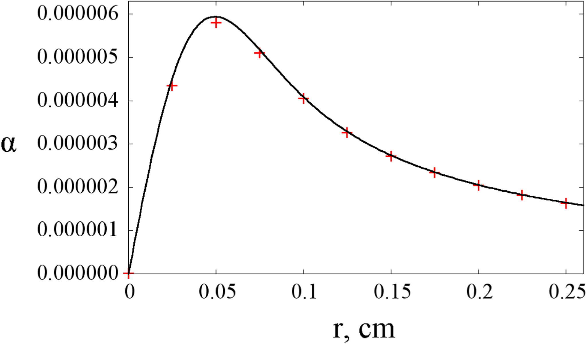
 $$\begin{eqnarray}{\it\alpha}=\frac{p_{r}}{p_{z}}=\frac{2Ne^{2}}{p_{z}rc}(1-\text{e}^{r^{2}/(2{\it\sigma}^{2})}).\end{eqnarray}$$
The analytical and numerical solutions for the deflection angle.

For cylinder length
 $l=0.05~\text{cm}$
, radius
 $R=3{\it\sigma}$
and where
 ${\it\sigma}=6.25\times 10^{-2}~\text{cm}$
, the beam charge
 $Q_{beam}=-Ne$
, beam population
 $N=10^{10}$
, the charge of the particle is
 $Q_{part}=e=4.8\times 10^{-10}$
esu and the relativistic factor of all the particles
 ${\it\gamma}=6.85\times 10^{3}$
, the grid used is
 $40\times 40\times 40$
with spatial step
 $h_{x}=h_{y}=0.025~\text{cm}$
,
 $h_{z}=0.0025~\text{cm}$
, time step
 ${\it\tau}=5\times 10^{-4}=1.66\times 10^{-3}~\text{ns}$
and the number of model particles in the beam is
 $J=4\times 10^{6}$
.
Figure 3 demonstrates the absolute values of the analytical solution (line) and the numerical solution (crosses) for the deflection angle dependence from the initial particle shift from the beam centre. The numerical results were obtained on a personal computer and show a good accuracy with commensurate speed for the given parameters using only
 $N_{{\it\tau}}=90$
time steps. However, simulations of focused beams with a highly nonlinear beam density distribution in space and time require significantly longer computations.
Let us consider the dynamics of two colliding flat beams moving along the
 $z$
-axis, one beam consists of monoenergetic electrons and the other consists of monoenergetic positrons. The particle density is distributed in the cross-over plane according to the Gaussian law:
 $$\begin{eqnarray}\displaystyle {\it\rho}(X,Y,Z)=\frac{1}{(2{\rm\pi})^{3/2}({\it\sigma}_{x}^{\ast }{\it\sigma}_{y}^{\ast }{\it\sigma}_{z}^{\ast })^{1/2}}\exp \left[-\frac{1}{2}\left(\frac{(X-X_{c})^{2}}{{\it\sigma}_{x}^{\ast 2}}+\frac{(Y-Y_{c})^{2}}{{\it\sigma}_{y}^{\ast 2}}+\frac{(Z-Z_{c})^{2}}{{\it\sigma}_{z}^{\ast 2}}\right)\right], & & \displaystyle \nonumber\\ \displaystyle & & \displaystyle\end{eqnarray}$$
where
 ${\it\varepsilon}_{x}=5\times 10^{-5}~\text{cm}$
and
 ${\it\varepsilon}_{y}=5\times 10^{-7}~\text{cm}$
are the horizontal and vertical beam emittances, respectively,
 ${\it\beta}_{x}^{\ast }={\it\beta}_{y}^{\ast }=0.1~\text{cm}$
are the corresponding beta-function values,
 ${\it\sigma}_{x}^{\ast }=\sqrt{{\it\beta}_{x}^{\ast }{\it\varepsilon}_{x}^{\ast }}$
,
 ${\it\sigma}_{y}^{\ast }=\sqrt{{\it\beta}_{y}^{\ast }{\it\varepsilon}_{y}^{\ast }}$
are the transversal beam sizes, the sign * denotes the values in the interaction point,
 ${\it\sigma}_{z}=0.1~\text{cm}$
is the beam size along
 $z$
-axis and
 $(X_{1_{c}},Y_{1_{c}},Z_{1_{c}})=(0,0,-0.35)~(\text{cm})$
,
 $(X_{2_{c}},Y_{2_{c}},Z_{2_{c}})=(0,0,0.35)~(\text{cm})$
are the beam centre coordinates in the cross-over plane. The momenta are defined by the Gaussian law:
 $$\begin{eqnarray}{\it\rho}(X^{\prime },Y^{\prime })=\frac{1}{2{\rm\pi}{\it\sigma}_{p_{x}}^{\ast }{\it\sigma}_{p_{y}}^{\ast }}\exp \left[-\frac{1}{2}\left(\frac{{X^{\prime }}^{2}}{{\it\sigma}_{p_{x}}^{\ast 2}}+\frac{{Y^{\prime }}^{2}}{{\it\sigma}_{p_{y}}^{\ast 2}}\right)\right],\end{eqnarray}$$
where
 ${\it\sigma}_{p_{x}}^{\ast }=\sqrt{{\it\varepsilon}_{x}^{\ast }/{\it\beta}_{x}^{\ast }}$
,
 ${\it\sigma}_{p_{y}}^{\ast }=\sqrt{{\it\varepsilon}_{y}^{\ast }/{\it\beta}_{y}^{\ast }}$
. The focusing condition is set as:
 $$\begin{eqnarray}\displaystyle & \displaystyle x=X+(z-z_{c})X^{\prime } & \displaystyle\end{eqnarray}$$
 $$\begin{eqnarray}\displaystyle & \displaystyle y=Y+(z-z_{c})Y^{\prime } & \displaystyle\end{eqnarray}$$
 $$\begin{eqnarray}\displaystyle & \displaystyle z=Z+z_{c} & \displaystyle\end{eqnarray}$$
 $$\begin{eqnarray}\displaystyle & \displaystyle p_{x}=p_{z}X^{\prime } & \displaystyle\end{eqnarray}$$
 $$\begin{eqnarray}\displaystyle & \displaystyle p_{y}=p_{z}Y^{\prime }. & \displaystyle\end{eqnarray}$$
The interaction point coordinates in the laboratory system coincide with the domain centre
 $(x_{c},y_{c},z_{c})=(0.05,0.005,0.75)~(\text{cm})$
, the relativistic factor
 ${\it\gamma}=6.85\times 10^{3}$
and the charge
 $Q_{1}=-Q_{2}=Ne=10^{12}e$
.
Unlike the model experiment with a cylinder beam, the focused beam has different sizes in the transversal directions and the ratio of the longitudinal and the transversal sizes of the focused beams is usually quite high. In the present case, the ratio is
 ${\sim}10^{2}$
, the computational region sizes in dimensionless units are
 $L_{x}=10^{-1}~\text{cm}$
,
 $L_{y}=10^{-2}~\text{cm}$
and
 $L_{z}=1.5~\text{cm}$
. We have to use a spatial grid of higher resolution and, as a consequence, a smaller time step because of the stability condition: the spatial grid is taken as
 $100\times 100\times 100$
, the time step
 ${\it\tau}=5\times 10^{-5}=1.66\times 10^{-4}~\text{ns}$
and the number of time steps
 $N_{{\it\tau}}=1.4\times 10^{5}$
. The number of model particles in each beam
 $J=10^{8}$
. The time of the beam interaction is
 $5T$
and the whole beam motion last
 $7T$
, where
 $T=2000{\it\tau}=0.33~\text{ns}$
.
The beam interaction regime can be characterized by disruption parameters (Chen & Yokoya Reference Chen and Yokoya1988), defined as
 $D_{x}=(2r_{e}N{\it\sigma}_{z})/({\it\gamma}{\it\sigma}_{x}({\it\sigma}_{x}+{\it\sigma}_{y}))$
and
 $D_{y}=(2r_{e}N{\it\sigma}_{z})/({\it\gamma}{\it\sigma}_{y}({\it\sigma}_{x}+{\it\sigma}_{y}))$
, where
 $r_{e}$
is the classical electron radius. The case of
 $D\ll 1$
corresponds to the non-critical regime, when one beam acts as a thin lens on the other beam. The case of
 $D\gg 1$
corresponds to the critical regime, when the beams disrupt each other. The given beam parameters correspond to the precritical regime of the beam–beam interaction, since the horizontal and vertical disruptions parameters are
 $D_{x}\sim 1.5$
and
 $D_{y}\sim 15$
. Figure 4 shows the coordinates
 $(z,y)$
of one beam at different time points. The critical beam density leads to beam deformation along the
 $y$
-axis after the interaction: the strong field of the oncoming beam additionally focuses the beam. The horizontal field is not as strong because of the bigger beam sizes in the
 $x$
direction, and there are no visible changes from the unperturbed beam dynamics (see figure 5).
The beam coordinates
 $(z,y)$
.

The beam coordinates
 $(z,x)$
.

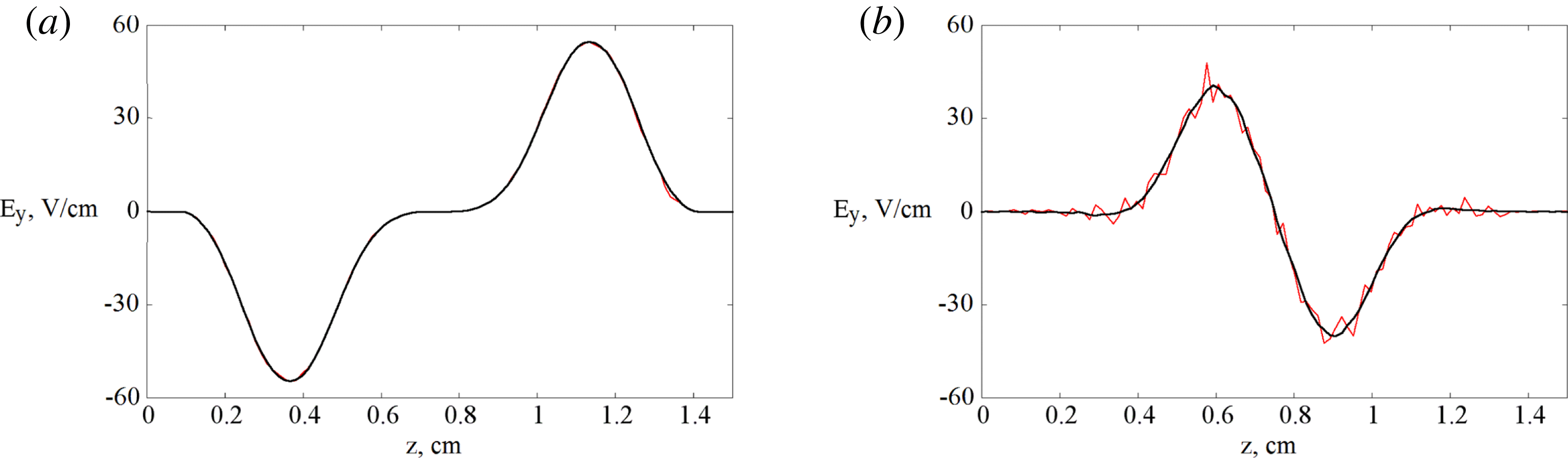
The electric field,
 $t=0$
(a) and
 $t=5T$
(b).

A monoprocessor machine allows us to perform simulations with a maximum
 $2\times 10^{6}$
model particles in the processor, which is not enough for such thin and long focused beams. A bigger number of particles cannot be used in the case of linear decomposition (
 $N_{g}=N$
) with a small number of groups: the central processors must compute almost half of the total number of particles because of the ‘hour-glass’ effect; it is more efficient to add a few processors to the central groups rather than to distribute them along the line.
Figure 6 shows the electric field in the plane
 $x=0.018~\text{cm}$
,
 $y=0.0025~\text{cm}$
for different numbers of model particles in each beam. Figure 6(a) relates to the time moment
 $t=0$
, where the lines coincide, the right-hand panel relates to the time moment
 $t=5T$
. The bold line corresponds to the case of
 $J_{1}=J_{2}=10^{8}$
and the thin polygonal line represents simulations with
 $J_{1}=J_{2}=10^{6}$
particles. We see that despite the smoothness of the field in the initial moment, the inadequate number of particles results in numerical errors.
In the case of supercritical parameters, these effects are stronger. Let the beam parameters remain the same, but the beam charge be 10 times higher:
 $Q_{1}=-Q_{2}=10^{13}e$
, hence the disruption parameters are
 $D_{x}\sim 15$
,
 $D_{y}\sim 150$
. Figure 7 demonstrates the beam coordinates
 $(z,y)$
at the time moment
 $t=5T$
in simulations with
 $J=10^{6}$
model particles (a) and with
 $J=10^{8}$
model particles (b). The computation errors interact with the developing physical instability and change the symmetrical beam shape.
The beam shape,
 $J=10^{6}$
(a) and
 $J=10^{8}$
(b).

The computations for
 $10^{8}$
particles in each beam lasted 6 h. The processors were divided into
 $N_{g}=25$
groups. The minimal possible number of cores to accommodate the particles was
 $N=240$
cores.
The parallel code demonstrated good efficiency and scalability (Boronina & Korneev Reference Boronina and Korneev2013). However, the refinement of the spatial grid in the
 $y$
direction, e.g. by doubling it, demands halving the time step because of the stability condition requirement. We draw attention to the number of particles needed in the simulations to avoid non-physical effects (Lotov et al.
Reference Lotov, Timofeev, Mesyats, Snytnikov and Vshivkov2015), namely, more than double the number of particles are required for smoothness of the particle density and currents due to the Gaussian particle distribution and the 3-D nature of the problem. The particles must be distributed in the same number of groups, in this case a minimum
 ${\sim}1200$
cores are needed to allocate the whole data in the memory. Flat beams require much greater supercomputer resources and are topical for further developments.
All the computations were performed on the Siberian Supercomputer Center cluster (ICM&MG SB RAS, Novosibirsk), 576 4-core processors Intel Xeon X5570/X5670 and the supercomputer Lomonosov (MSU, Moscow), 12346 4-core processors Intel Xeon X5570/X5670.
5. Conclusion
We have presented a new fully 3-D model and corresponding parallel code for beam–beam simulation for the case of high relativistic factors (
 $10^{3}{-}10^{5}$
). The algorithm is based on the Vlasov equation solution with the PIC method. The mixed domain and particle decomposition enables us to perform numerical experiments for beams with a size ratio 10:1:100 using spatial grid
 $100\times 100\times 100$
and a particle number
 $10^{8}$
, which cannot be obtained using monoprocessor machines or usual linear domain decomposition. The results demonstrate quantitative agreement with the existing analytical solution for particle deflection in the field of a cylindrical Gaussian beam and are in qualitative agreement in cases of colliding beams with critical densities. The presented algorithms and methods are applicable to a variety of problems in relativistic plasma physics, for example, plasma heating by relativistic electrons in nuclear fusion and wakefield acceleration by proton (electron) bunch driven plasma.
Acknowledgement
The support of the Russian Scientific Foundation grant 14-11-00485 ‘High performance methods and technologies of modelling the electrophysical processes and devices’ is gratefully acknowledged.