In 1850 manufacturing employed approximately 15 percent of the American labor force. Except in a few industries such as cotton textiles, the typical establishment then was a sole proprietorship with perhaps one hired hand. In such “artisan shops” the owner worked alongside his employee(s), fashioning each unit of output from start to finish. Use of inanimate power sources was atypical in artisan shops and the capital intensity was relatively low.
Fifty years later, manufacturing had increased its share of total employment to 20 percent and, although the artisan shop remained common, an increasing proportion of production originated in factories.1
The figures in the text on the proportion of the labor force engaged in manufacturing are computed from U.S. Department of Commerce, Historical Statistics, series 167 and 174, p. 139. On the (slow) demise of the artisan shop see Atack and Bateman (“Preliminary Data on the Spread”).
These generally differed from artisan shops in three ways—they had many more workers, they used more capital per worker, and they were more likely to use an inanimate power source.
2 For example, in 1895 the machine production of 12 dozen men's white muslin shirts employed 39 different operations, 18 of them assisted by steam power, in a factory employing 230 workers, compared with 25 hand operations in an artisan shop in 1850 with just a single employee. The change in production methods cut the total production time by a factor of 7.6 (1,439 hours were needed to produce 12 dozen shirts in 1853 compared with 188.2 hours in 1895). See U.S. Department of Labor, “Hand and Machine Labor,” pp. 1094–97.
The diffusion of the factory produced dramatic gains in output per worker such that, by century's end, American manufacturers were already (or were poised to become) world leaders in a wide array of industries.
3 Chandler, Visible Hand; Wright, “Origins”; and Engerman and Sokoloff, “Technology.”
Although economic historians generally agree that the diffusion of the factory generated gains in labor productivity, there is less agreement on its effects upon the skill level of the manufacturing labor force. One point of view is that the manufacturing labor force was “de-skilled” by the diffusion of the factory.4
See, for example, Brown and Phillips, ”Craft Labor.”
A case can be made for de-skilling on
a priori grounds because the factory system clearly achieved some of its gains in labor productivity through the division of labor and standardization of products.
5 Hounshell, From the American System; and Sokoloff, “Was the Transition.”
The subdivision of production into a series of simpler tasks made each easier to learn, to master, and to mechanize, particularly when the product was standardized. Thus, division of labor shortened the period of skill acquisition—in extreme cases, to the point where tasks might be learned in a matter of days or even hours—as well as lessening the degree of skill and dexterity required. As one turn of the century commentator put it, “[t]hrough the simplification of mechanical processes ignorant labor is congregated in factory centers… the ignorant masses are enabled… [t]o engage in what it once took skilled labor to perform….”
6 U.S. Census Office, “Factory System,” p. 566.
The growth of manufacturing after 1850, however, was also accompanied by an increase in capital per worker and in the use of inanimate power sources, particularly steam and, after the turn of the century, electricity. This higher level of capital and energy use reflected the installation of machines, and these activities were complementary to skilled labor, such as that of engineers. Moreover, larger, more complex enterprises required the documentation of economic activities by the firm and these activities were complementary to white-collar skills. Furthermore, as the factory system developed, the diversity and complexity of products increased.7
Scranton, Endless Novelty.
Many of these new products may also have required novel skills or highly specialized work forces.
As Daron Acemoglu has recently pointed out, economic historians have made relatively little progress on the de-skilling hypothesis because direct empirical evidence of any kind linking skill intensity to the characteristics of manufacturing establishments is scarce prior to the twentieth century.8
Acemoglu, “Technical Change.”
Instead, scholars have relied upon indirect evidence and inference. For example, using establishment-level data from 1820 to 1850, Claudia Goldin and Kenneth Sokoloff show that the percentage of workers who were children or young women—which they use as a proxy for lower skill intensity—rose with establishment size.
9 Goldin and Sokoloff, “Women” and “Relative Productivity Hypothesis.”
However, although such evidence is clearly valuable, not all industries or establishments hired women and children, and the proportion of such workers among all manufacturing workers peaked well before the end of the nineteenth century.
In this article we use evidence drawn from the handwritten enumerations of the 1850 and 1880 censuses to shed new light on skill intensity and its determinants in nineteenth-century manufacturing. Our analysis ceases with 1880 because establishment-level data for the 1890 and 1900 manufacturing censuses no longer exist.10
For a detailed description of the data collection process, see Atack and Bateman “U.S. Historical Statistics.” The manuscript records of the 1890 census of manufacturing were destroyed by fire and those for 1900 were disposed of by act of Congress. Data are also available for 1820, 1860, and 1870 (see Sokoloff, “Was the Transition”; and Atack and Bateman, “U.S. Historical Statistics”) but, as our focus is on broad changes over time, we chose to use the beginning and end dates of the Atack-Bateman samples.
Our evidence consists of average monthly wages paid by manufacturing establishments—the “establishment” wage—and establishment characteristics. As in Goldin and Sokoloff's case, our evidence is indirect. Consequently our interpretation of it rests heavily on a model—specifically, the model of manufacturing put forth recently by Goldin and Lawrence Katz.
11 Goldin and Katz, “Origins.”
In the Goldin-Katz model, skill intensity in manufacturing is determined by establishment size, capital intensity, and energy use, and it is the correlations of these variables with the establishment wage—itself a proxy for average skill—that we explore. Goldin and Katz tested their model using wage data from the twentieth century, but, to our knowledge, such a test has not been applied previously to nineteenth-century data.
Our findings are broadly supportive of the de-skilling hypothesis. In particular, we show that the average wage was a decreasing function of establishment size, as measured by employment, in both 1850 and 1880. The negative wage–size gradient is precisely what is predicted by the Goldin-Katz model and is consistent with the hypothesis that skill intensity decreased as establishment size increased. We also show that capital-intensive establishments and those using steam power had higher average wages, which, in terms of the model, implies that these establishments used relatively more skilled labor, other factors held constant. Thus, although the diffusion of the factory reduced skill intensity through its positive association with establishment size, these negative effects were offset to some degree by growth in capital per worker and greater reliance on inanimate power sources, which tended to raise skill intensity. Overall it appears that the manufacturing labor force was de-skilled because the employment-weighted distribution of average wages was much more unequal below the median wage in 1880 than in 1850—that is, there were relatively more workers employed in establishments with low establishment wages in 1880 than in 1850. Using a decomposition analysis, we demonstrate that an economically significant proportion of the increase in wage inequality below the median can be accounted for by the growing concentration of all employment in large establishments, which, according to both the Goldin-Katz model and our wage regressions, had relatively unskilled workforces.
A MODEL OF MANUFACTURING
We sketch a simple model of manufacturing that is essentially identical to the model of Goldin and Katz.12
Goldin and Katz, “Origins.”
The goal is to provide intuition for our empirical work linking average wages to establishment characteristics.
The model presumes that industrialization proceeded in three distinct phases—from “artisan shop” (phase 1) to “factory” (phase 2) to “continuous processing” (phase 3). The focus of the model is principally on differences in outcomes—for instance, skill intensity—between the phases rather than on the economic fundamentals that propel the transition from one phase to the next.13
Goldin and Katz, however, clearly have various economic fundamentals in mind. For instance, to the extent that the “division of labor [was] limited by the extent of the market” falling costs of transportation (railroads, canals, and so on) was a factor behind the transition to the factory—as were technological advances, such as steam, that increased the productivity of unskilled labor. Improvements in capital markets, as reflected in reductions in the rental price of capital, may have been an additional factor; see Atack, Bateman, and Margo, “Capital Deepening.”
Because the continuous-process phase occurred largely after the turn of the twentieth century and because our empirical analysis stops with 1880 when establishment-level data cease being available, our exposition focuses on the first two phases.
Within each phase, the manufacturing process is divided in two stages. In the first stage, skilled labor (Ls) is combined with “raw” capital (Kr) to produce, install, and subsequently maintain an intermediate input called “operating” capital (Ko). This may include machines, for instance, with a range of capabilities and degrees of specialization and specificity. For simplicity, and following Goldin and Katz, we presume the production function for operating capital in this stage is Leontief, which, without loss of generality, we write as follows
In the second stage, operating capital is combined with unskilled labor (Lu) to produce a finished good (q). Substitution between operating capital and unskilled labor is permitted in the second stage as, for example, with a Cobb-Douglas technology.
14 As Goldin and Katz (“Origins,” p. 700) point out, the Leontief assumption can be relaxed without altering the qualitative implications of the model so long as no unskilled labor is used in the first stage.
We assume that, for any given level of q, firms minimize costs. In the second stage, the solution to the cost minimization problem yields an optimal ratio of unskilled labor to operating capital that is a function (Φ) of the ratio of the rental price of operating capital to the unskilled wage (f=r/wu) and, possibly, of the level of output
Let S be skill intensity, S=Ls/(Lu+Ls). It follows that
In the typical artisan shop α is presumed to be large and Φ is presumed to be small. When α is large, relatively large amounts of skilled labor are needed per unit of raw capital to produce a unit of operating capital. Whereas the overall capital requirements in an artisan shop might be minimal, each artisan customarily maintained his own tools, implying a high value of α. In the typical artisan shop final products were made to order, and a significant portion of the operating capital might consist of inventories of partially completed goods made by the most skilled workers, with finishing touches applied by apprentices.15
Goldin and Katz, “Origins,” p. 701.
Thus, in the typical artisan shop, Φ would be small. As the equation for skill intensity shows, when α is large and Φ is small, skill intensity will be relatively high.
Factories are distinguished from artisan shops in using (at given factor prices) higher ratios of unskilled labor to operating capital in the second stage of production and higher ratios of raw capital to skilled labor in the first stage. That is, factories substitute capital and unskilled labor for skilled labor: relatively less skilled labor per unit of raw capital is used in the first stage (a low value of α), but relatively more unskilled labor per unit of operating capital in the second stage (a high value of Φ).
We think of the greater relative use of unskilled labor per unit of operating capital as the essence of division of labor. Through the division of labor, factory owners subdivided the tasks of the second stage of production so that tasks could be performed by an unskilled worker using a machine or piece of specialized equipment. In terms of the model, Φ is relatively high in the typical factory for any given value of α or q.
Factories are also distinguished from artisan shops by requiring less skilled labor per unit of raw capital in the first stage. This could be because, as noted, each artisan maintained his own tools, whereas in the factory a single worker (or a small number thereof) installed and maintained the machines operated by the unskilled workers in the second stage. Thus, in the factory α will be relatively low. As the equation for S shows, when α is low and Φ is high, S, skill intensity, will be low.
Although the model predicts that skill intensity will be lower in the factory than in the artisan shop, whether the ratio of operating capital to total employment [k=Ko/(Ls+Lu)] is higher or lower depends on the precise values of α and Φ. However, it is straightforward to show that k=S/α.16
By definition, k=(Ko/Ls) × S=S/α. Note that both S and α are smaller in the factory than in the artisan shop. Consequently, according to the model, capital intensity may be higher or lower in the factory than in the artisan shop depending on the values of α and Φ (because S is a function of α and Φ); see Goldin and Katz, “Origins”; and Atack, Bateman, and Margo, “Capital Deepening.”
That is, skill intensity should be positively correlated with capital intensity, an implication of the model that we test in the next section.
The third phase of industrialization, continuous processing, differs from the factory phase primarily in the second stage of production, in that a vastly higher ratio of capital to unskilled labor was the norm. According to Goldin and Katz, the critical technological advance was the development and diffusion of electrical power. Electricity greatly altered the design of manufacturing plants, permitting the elimination of a wide range of unskilled jobs on the shop floor that were involved in the movement of bulky raw materials and goods in process from one location to another in the plant. Consequently, continuous processing establishments tended to be relatively more skill intensive than factories even though, in terms of employment, they could be much larger in size than factories.
With very few exceptions, the diffusion of continuous processing technology did not begin in earnest in American manufacturing until after about 1900.17
The major exceptions are reduction flour milling and cigarettes, both of which used continuous processing techniques after 1880; see Chandler, Visible Hand.
However, the diffusion of electricity was temporally preceded by the diffusion of steam power. Measured by horsepower, use of steam in manufacturing increased by nearly sixty-fold from the late 1830s to the late 1870s.
18 Fenichel, “Growth and Diffusion,” table A-1. On the diffusion of steam power in manufacturing, see Atack, Bateman, and Weiss, “Regional Diffusion.”
The diffusion of steam did not alter the architecture of production in the same manner as the diffusion of electricity. However, steam engines and the millwork that they powered were highly complex machines that required installation, regular maintenance, and trouble-shooting. In terms of the model, the use of steam may have required relatively more skilled labor per unit of raw capital in the first stage of production (a high value of α) and may, as well, have involved relatively more capital per unskilled worker in the second stage (Φ), implying a higher overall level of skill intensity. We explore the possible effects of steam use on skill intensity in our empirical analysis in the next section.
Goldin and Katz tested their model using industry-level data from the early twentieth century by regressing the logarithm of the average annual wage on industry characteristics such as size, capital intensity, and electricity use. The idea behind this test is straightforward: industries with a higher level of skill intensity should have higher average wages—that is, Goldin and Katz use the average wage as a “sufficient statistic” for skill intensity. The empirical analysis in the next section follows Goldin and Katz, but with three differences. First, our analysis is conducted using establishment-level data rather than industry averages. Second, the dependent variable in our analysis is the logarithm of the average monthly wage. We use average monthly wages rather than average annual wages because the annual wage bill was not reported prior to the Civil War. Third, as just noted, we control for the use of steam power—the relevant motive power that diffused after 1850—whereas Goldin and Katz are interested in the effects of electricity use on average wages.
REGRESSION ANALYSIS OF ESTABLISHMENT WAGES
In this section we report regressions of the average monthly wage—the “establishment wage”—on establishment-level characteristics. Our analysis, like that of Goldin and Katz, presumes that the average wage is a proxy for skill intensity, and we interpret the regression coefficients in light of the model of manufacturing sketched in the previous section. The data come from samples from the manuscript censuses of manufacturing for the census years 1850 and 1880.19
These samples are random and nationally representative of the universe of surviving manuscript schedules. Each sample contains data on several thousand establishments. Census enumerators collected the original data through personal inquiry of knowledgeable parties (such as the owner). The data pertain to economic activities from June of the prior year through May of the census year.
The two censuses differ somewhat in terms of the wage and employment information reported in them. In 1850 enumerators collected data on the average number of male and female workers employed and on the average total monthly wages paid to each group. The goal was “that by dividing the latter by the former the result will show the average [monthly] earnings of individuals.” The exact meaning of “average” was not clearly specified but a plausible reading is that “average” meant during a “typical” month, which (in order to make comparisons with 1880) we interpret in full-time equivalent terms. In 1880 enumerators collected data on the total annual wage bill rather than the average monthly bill. Employees were classified into adult males (over age 16), adult females (over age 15), and children of both sexes. Although information on full-versus part-time status is not available in 1850, it is possible to deduce full-time equivalent months of operation in 1880 from a series of questions on operating times.20
The 1880 census reported months of operation on half-time, on two-third's time, on three-quarter's time, and on full-time. We define full-time equivalent months to be months on full-time+0.75*months on three-quarter's time+0.67*months on two-third's time+0.5*months on half-time.
From this description it is clear that the average annual wage can be constructed in 1880 but not in 1850. For consistency, therefore, we specify the dependent variable to be the log of the average monthly wage. The average monthly wage in 1850 is
The average monthly wage in 1880 is
Inspection of the wage distribution in both years reveals observations for which the value of the average monthly wage is either too low or too high to be credible. Studies using twentieth-century wage data often impose bounds on the distribution in order to minimize the impact of severe outliers.
21 See, for example, Katz and Murphy, “Changes in Relative Wages.” For a subsample of establishments, the 1880 census reported the average daily wages of “unskilled labor” and “mechanics.” We use this information to construct lower and upper bounds on the distribution of the average monthly wage. Specifically we assume that the lowest credible average monthly wage in 1880 is equal to the lowest observed daily wage of unskilled labor (20 cents) multiplied by a full-time month of 26 days (see Atack, Bateman, and Margo, “Part-Year Operation”). The upper bound is set equal to the highest observed daily wage of mechanics times 26 days per month. Lower and upper bounds for 1850 are constructed by adjusting the 1880 bounds by the change in an overall index of manufacturing prices between 1850 and 1880; see Atack, Bateman, and Margo, “Capital Deepening.” Approximately 5 percent of the observations in both years are excluded by imposing these bounds. We experimented with different trimming procedures (for example, deleting the bottom 1 and top 99 percent of establishments based on their average wage) but our substantive results were not affected.
We follow a similar approach here and exclude wage values outside certain bounds (see the notes to
Table 1).
In addition to “trimming” the data of outliers, we imposed two other selection criteria. We dropped the relatively small number of establishments in the far West, the majority of which were in California. In 1850, of course, California was in the midst of the Gold Rush and there is good evidence that wages were temporarily very high.22
Second, we deleted establishments for which the gross value of output was less than five hundred dollars. In principle such establishments should not have been enumerated in either year, but some clearly were. As we have no way of knowing whether these were representative or not, we elected to delete them.
There are also two potential sources of bias worth noting. The first concerns the reporting of the earnings and labor input of owners of manufacturing establishments. To the extent that owners labored alongside their employees—there is no question this was true in artisan shops—they should be included in the analysis. However, the extent to which the census data actually accurately reflect earnings and the entrepreneurial labor input is unclear—particularly, as it happens, in 1880.23
If the entrepreneurial labor input were not counted and valued, then the average wage in very small establishments would be biased downwards for (at least) two reasons. First, the owners of such establishments were almost certainly more skilled than their workers (some of whom could be apprentices) and second, hired labor in very small establishments may have been employed part-time rather than full-time. We can control for months of operation in 1880 (see the text) but this is not the same as controlling for labor time of employees.
The instructions to enumerators in 1850 and 1860 clearly specify that the labor input of owners should be counted and those for 1860 state that the “earnings” of the owner were to be included in the wage bill; see U.S. Census, Seventh Census, p. xxiv, and U.S. Census, Eighth Census, p. 27. The 1880 instructions, by contrast, did not specify how the labor input of the owner was to be treated. Of course, what enumerators did in practice may have differed from the instructions, and some scholars have contended that the labor input of owners was systematically under-reported; see, for example, Sokoloff, “Was the Transition.”
If the instructions were not followed, we should observe very small establishments reporting posi-tive outputs but no “workers.” These would be establishments in which all the work was done by the (single) owner. In 1850 there are only a handful of establishments falling into this category. In 1880, however, there is a small, but nontrivial proportion of such establishments; see Atack, Bateman, and Margo, “Capital Deepening.” Consequently, if there is a downward bias in the average wage in very small establishments because of the under-reporting of the labor input of owners, we believe it is likely to be worse in 1880 than in 1850. In this regard, we note that the average wage in 1880 increases in going from 1–5 to 6–15 workers after controlling for other factors. This is not the case in 1850 and this is exactly the pattern that would be expected if there were a downward bias in 1880 but not in 1850.
Because this problem is especially salient for the very smallest establishments in our analysis (1–5 workers) it is possible that the average wage for these establishments, if calculated as above, is measured with error—specifically, the wage may be biased downwards. For this reason our interpretation of the results, specifically the relationship between size and the establishment wage, focuses on patterns revealed by differences between size classes at 6–15 workers and above rather than on comparisons with the very smallest establishments.
Second, in an effort to secure more and better information for certain specific industries in 1880, the data for these industries were to be collected by “special agents” rather than by the regular enumerators. These agents were chosen for their special knowledge of the industries. Unfortunately, the manuscript schedules collected by these special agents have never been found and are presumed lost. In practice, however, the distinction between special agent and regular enumeration was blurred, and regular enumerators did, in fact, collect data from establishments in the special agent industries (presumably, by mistake). When chosen by the (random) sampling procedure, these were included in the samples but there is no question that the special agent industries are under-represented in 1880. On the assumption that special agent establishments that happened to be canvassed by regular enumerators were not systematically different from the underlying population, it is possible to correct the 1880 data for the under-enumeration.24
See Delle Donne, “Federal Census Schedules.” A list of the special agent industries and the details of the reweighting are available on request from Robert A. Margo. In brief, we scale up employment in special agent industries in 1880 such that the proportion of workers in such industries in 1880 was equal to the average proportion in the 1850–1870 samples. Plausible variations on this reweighting (for example, allowing for a trend in the weight) do not change our substantive findings.
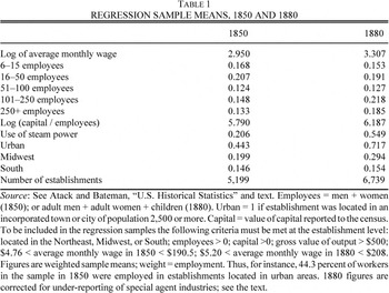
Table 1 shows the sample means for the dependent variable and key independent variables, except for industry dummies (included in some specifications). The Goldin-Katz model does not define the “factory” precisely in terms of a level of employment, nor does it specify a precise functional form linking skill intensity to size. We experimented with a variety of ways to control for size including nonparametric approaches. For simplicity, we settled on a set of dummy variables for size categories, as shown in Table 1, the smallest being 1–5 workers and the largest being 250 or more. We also estimated regressions with a linear term in employment, as these are easily compared across specifications.25
The linear term is the number of workers/100; see Table 2 and various footnotes. Sokoloff (“Was the Transition”) finds an increase in total factor productivity comparing establishments with 6+ workers to those with 1–5 workers.
The smaller size dummies are the same as those used by others such as Goldin and Sokoloff.
26 In nominal terms, the log of the average monthly wage in 1880 was 0.357 points higher than in 1850, a difference of about 42 percent.
27 42 percent=exp [3.307 – 2.950] × 100.
Capital intensity—measured as the value of capital reported divided by total employment, and also in nominal terms—increased over the same period, as did the proportion of individuals working in establishments using steam. Establishment size rose as well, entirely because of increases in the proportion of workers employed in the three largest size classes (51–100, 101–250, and 250+workers).
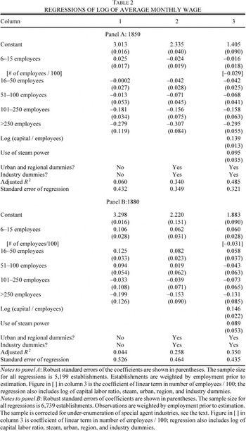
Coefficients of the key independent variables—the size dummies, capital intensity, and use of steam power—are reported in Panels A (1850) and B (1880) of Table 2. The regressions fit the data reasonably well, and (not surprisingly) the fit improves as we add covariates.
Column 1 reports regressions in which the only independent variable is size. Even with such a minimal specification, we can observe a negative wage-size gradient above the first size class (6–15 workers) in both years.28
If individuals required a compensating differential to work in factories, as opposed to artisan shops, our regressions may understate the degree to which skill intensity declined with establishment size. We cannot investigate this possibility in 1850, but in 1880 the census also reported the average daily wage of common labor and “mechanics” for a subsample of establishments. Regressions of the log of daily wages using the column 3 specification in Table 2 show that daily wages of both types of workers were higher in establishments employing six or more workers than in the very smallest establishments, but there is little evidence of an additional gradient with respect to size, except possibly for skilled labor in the largest establishments. These additional regressions are available on request from Robert A. Margo.
In 1880, for instance, the average wage in the largest establishments (250+ workers) was approximately 26 percent lower than in the 6–15 size class, the same as in 1850.
29 Sokoloff and Villaflor (“Market”) report regressions of average wages in 1850 that display little relationship between wages and size, unless size is interacted with location; see their table 1.4, equations 5 and 6. However, there are several differences between Sokoloff and Villaflor's analysis and ours. First, Sokoloff and Villaflor's dependent variable is the estimated adult male wage. This variable is estimated, because the 1850 census did not distinguish between boys and adult males. Consequently, Sokoloff and Villaflor assumed that industries in 1850 employed boys in the same proportion to men as in 1820, and that the boy wage was 50 percent of the adult male wage. Because the 1850 census did report total monthly wages paid to males, these assumptions are sufficient to estimate the adult male wage. Sokoloff and Villaflor use the adult male wage because their focus is on market integration for which it is important, as much as possible, to hold skill intensity constant across establishments in different locations, whereas our focus is on variations across establishments in skill intensity. Secondly, Sokoloff and Villaflor restrict their analysis to the Northeast, whereas our analysis covers the entire country. Third, and perhaps most importantly, Sokoloff and Villalfor used an earlier version of the Atack-Bateman 1850 dataset that was smaller in size and not representative either regionally or nationally—and, therefore, not self-weighting (the national samples that we use became available only after Sokoloff and Villalfor wrote their paper). For these reasons, especially the last, it may be next to impossible to fully reconcile differences between our 1850 findings and those of Sokoloff and Villaflor.
The column 1 specification does not control for the location of the establishment. Urban workers, for example, arguably faced higher costs of living than did rural workers, and there are good reasons to believe that the various census regions did not constitute a unified national market, either in 1850 or in 1880. For a variety of reasons, average wages may have varied across industries. Accordingly, in column 2, we add dummy variables for urban status, region, and industry. Although adding these controls improves the fit of the regression, it does not change the finding of a negative wage–size gradient.30
The location and industry coefficients are available from Robert A. Margo on request. With regard to location, we find that urban establishments paid higher average wages and southern establishments lower wages in both years. We find little difference in the regional structure of wages between 1850 and 1880; however, if we substitute the 1860 sample for the 1850 sample, we would find a rise in the North-South wage gap, consistent with previous work by Margo (“North-South Wage Gap”) and Wright (Old South). The magnitude of the urban coefficient is somewhat larger in 1880 than in 1850. As pointed out in the text, the proportion of workers employed in establishments located in urban areas increased between 1850 and 1880. To the extent that this shift reflected an increase in the relative demand for urban locations (and therefore, urban workers) it is possible that the premium needed to induce workers to locate in urban areas increased over time.
In column 3 we include the log of the capital-labor ratio and the dummy for steam power. In both years we observe positive and statistically significant effects of capital intensity and use of steam power. The positive coefficients are consistent with our model and in that context imply that skill intensity was higher in capital-intensive and steam-powered establishments. Inclusion of capital and steam in the regression does little to alter the negative relationship between wages and size. Overall, the “wage structure”—the coefficients of the size, capital intensity, and steam—appears to have remained approximately constant between 1850 and 1880, despite the shifts in the mean values of the independent variables.31
In particular, if we substitute a linear term (number of employees/100) for the size class dummies, the estimated coefficient on size is slightly larger in 1880 than in 1850, but this difference is not statistically significant (see Table 2).
We conducted three sensitivity tests. First, as noted above, there is some concern that the average wage in the smallest size class (1–5 workers) may be understated. Dropping these establishments from the samples dramatically reduces the sample sizes. However, the substantive findings—negative wage–size gradient, and positive effects of capital intensity and steam power use—remain unchanged. Second, the regressions do not control for the number of months of operation of the establishment (full-time versus part-time), yet there are good reasons to believe that part-time establishments, which were more likely to be small in size, may have had to pay a premium to attract workers.32
Atack, Bateman, and Margo, “Part-Year Operation”.
We can do nothing to control for months of operation in 1850 because such information was not collected then, but we can control for months of operation in 1880. Restricting the 1880 sample to establishments that operated on a full-time basis for the entire year (12 months) flattens the wage–size gradient, but the effect is very slight.
33 If the 1880 sample is restricted to establishments in operation for 12 full-time equivalent months, the coefficient of the linear term in employment is −0.026, compared with −0.031 in the full 1880 sample; see Table 2.
Third, we re-estimated the regressions including the percentage of workers who were female in 1850 and the percentage of workers who were adult females or children in 1880. Goldin and Sokoloff's analysis indicates that, in some industries, manufacturers implemented division of labor by substituting less skilled young women and children for adult men, and that the percentages of such workers were increasing in establishment size.
34 Goldin and Sokoloff, “Women.”
If so, adding the percentages of such workers to our regressions should attenuate the wage–size gradient, at least to some extent. In fact, this is case—if the variables are added, the size gradients in both years become smaller (i.e., flatter) in absolute value.
35 We say “to some extent” because female and children workers were not used in some industries. Specifically, if the female share of employees (=females/(males+females)) is added to the 1850 regression with the linear term in employment (employees/100) the coefficient declines from −0.029 to −0.015. If the share of adult women and children is added to the 1880 regression, the coefficient of the linear term in employment declines from −0.031 to −0.027. If we regress the percent female in 1850 or the percent adult women plus children in 1880 on establishment characteristics as in Table 2, column 3, we find a positive effect of size (use of female or child workers was increasing in establishment size), and negative effects of capital intensity and steam (use of female or children workers decreased as capital intensity increased or steam was used). These patterns are consistent with the Goldin-Katz model, treating the percent female or percent adult women plus children as a (negative) proxy for skill intensity. The regressions of percent female and percent women and children are available from Robert A. Margo on request.
In sum, the regressions results are strongly consistent with the Goldin-Katz model. The model predicts a negative relationship between size and skill intensity and, therefore, size and the average wage, and this is what we find. The model also predicts that capital-intensive establishments should have had higher average wages, and this is also what we find. Lastly, we hypothesized that steam-powered establishments may have used relatively more skilled labor, and this hypothesis is consistent with the higher average wage paid by establishments using steam power.
CHANGES IN THE DISTRIBUTION OF ESTABLISHMENT WAGES, 1850–1880
In the previous section we demonstrated that the establishment wage was a negative function of establishment size in 1850 and 1880. We interpreted this pattern as evidence that skill intensity was decreasing in establishment size, and therefore as evidence in favor of the de-skilling hypothesis.
It could be argued, however, that the de-skilling hypothesis is not just about the relationship between size and skill intensity at a point in time, but rather about a growing concentration of low-wage—and therefore, low-skill—workers in manufacturing. Although our data do not allow us to investigate changes in the distribution of wages of individual manufacturing workers they do permit us to trace changes in the distribution of the establishment wage over time. Further, by weighting each establishment by its employment, inequality in establishment wages is made (approximately) equivalent to the “between-group” component of overall wage inequality in manufacturing, where the grouping variable is the establishment. Using standard techniques, we can decompose changes in the (weighted) distribution into various components, including changes over time accounted for by changes in the distribution of employment across establishment size categories.
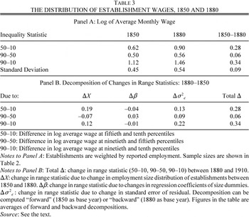
Panel A of Table 3 reports various range statistics of the distribution of log of establishment wage in 1850 and 1880. The range statistics indicate that wage inequality increased between 1850 and 1880. Most of the increase in inequality occurred below the median, as indicated by the substantial rise in the difference in the value of the log wage between the tenth percentile and the median—the 50–10 range statistic.
We use the regression results to compute a decomposition of changes over time in the range statistics into component parts, including the portion due to changes in the distribution of observable establishment characteristics, such as size.
36 For further discussion of decompositions of range statistics, see Katz and Murphy, “Changes”; and Juhn, Murphy, and Pierce, “Wage Inequality.”
We begin with the log wage specification as reported in
Table 2
In this equation, ln w represents the logarithm of the establishment wage, the X's are observable establishment characteristics, β is the vector of regression coefficients, σ is the standard deviation of the regression residuals (the standard error of the regression), and δ (=ε/σ) is the standardized residual. We have two cross-sections, and therefore two estimates of β and σ, one set corresponding to 1850 and the other to 1880.
For each observation in 1850 we use the regression results from 1880 to compute ln w*
That is, we multiply each establishment's observable characteristics (X) in 1850 by the 1880 regression coefficients and add this to the establishment's residual. By inspection it is clear that any difference between the range statistics of ln w1850 and ln w* is due solely to changes in β (=Δβ).
Next, we compute ln w**
The only difference between ln w* and ln w** is the substitution of the 1880 value of σ for the 1850 value. Therefore, any difference between the range statistics of ln w* and ln w** reflects changes over time in σ, the standard error of the regression (=Δσε2).
Lastly, any difference between the range statistics of ln w** and ln w1880 reflects changes over time in the distribution of X and in the mapping between X and δ (=ΔX). It is this last component that is of particular interest, because it is here that the impact of changes in the distribution of establishment size will be reflected.
Any decomposition requires a choice of a base year, as well as a regression specification (β and σ). Because the choice of a base year is arbitrary we computed both “forward” (1850 as the base year) and “backward” (1880 as the base year) decompositions. Panel B of Table 3 reports the average figures from the two decompositions using the simplest of the regression specifications reported in Table 2, which uses only the size dummies as the independent variables.37
Results using the other specifications are available from Robert A. Margo on request.
The findings in panel B indicate that shifts in the distribution of establishment size—in particular, the growing concentration of employment in large establishments—can explain a significant amount (68 percent=0.19/0.28) of the increase in wage inequality below the median—that is, in the 50–10 range statistic. However, these same changes imply that inequality above the median (the 90–50 range statistic) should have decreased whereas, in fact, inequality above the median increased. Consequently, the percentage of the total change in inequality (the 90–10 statistic) that is explained by the change in the distribution of employment is much less: 35 percent (=0.12/0.34). On the other hand, changes in the regression coefficients had little effect on overall inequality, reflecting their general stability over time. Much more important, however, was the increase in the standard deviation of the residuals; indeed, this term alone is slightly less than half of the growth in inequality below the median and two-thirds of the increase in overall inequality. Moreover, the relative explanatory power of the various terms does not change much if we alter the decomposition by including additional covariates.
By its very nature it is extremely difficult to explain the rise in residual wage inequality. In this regard, studies of changes in wage inequality in the late twentieth century frequently find increases in residual inequality, which are interpreted as evidence of a rise in the returns to “unobservable” skills such as “ability.”38
Juhn, Murphy, and Pierce, “Wage Inequality.” An alternative explanation is that there was a growing diversity of skills, conditional on establishment characteristics. We cannot rule this out because, unlike modern studies, we do not control directly for skills, only indirectly through proxies such as size, capital intensity, and so on. Any such increase in diversity would have to have been complex, in the sense that it could not have greatly affected differences in average wages across observable characteristics, such as size, because we observe relatively little change in the regression coefficients between 1850 and 1880. Scranton (Endless Novelty) argues that “specialty production” grew substantially in manufacturing after the Civil War and that such production involved new and diverse skills.
Wage data by occupation suggest that skill differentials may have increased between 1850 and 1880, so we cannot rule out such an increase in the returns to ability on
a priori grounds.
39 Williamson and Lindert, American Inequality. On the basis of our data, however, it is difficult to make a strong case for a rise in the returns to (observable) skill between 1850 and 1880. If such an increase took place, we should observe increases in the absolute values of the coefficients of size, capital intensity, and steam power use between 1850 and 1880, as these characteristics were correlated with skill intensity. We do find slight increases in the size and capital intensity coefficients (see, in particular, the linear term in size in Table 2); the coefficient on steam declines in magnitude and, in any case, the changes in the coefficients are small and not statistically significant. As previously noted, we do observe a positive correlation between wages and urban status, and a rise in the urban wage premium over time. This could be consistent with a rise in the skill premium although it might just as well reflect a rising cost of living in urban areas relative to rural areas.
However, documenting convincingly that such an increase actually took place would require far more information on the characteristics of individual workers than is commonly reported today in census data, much less for nineteenth-century manufacturing.
Our data, we reiterate, do not speak directly to whether the distribution of wages of individual manufacturing workers was becoming more unequal between 1850 and 1880, only that the distribution of average wages at the establishment level became more unequal. It is possible that the overall distribution of wages among manufacturing workers remained unchanged while the distribution of establishment wages became more unequal. Here, two points may be made. First, in the twentieth century, there is an impressive co-movement in establishment and individual-wage inequality in manufacturing—when individual wage inequality increases, so too does establishment wage inequality.40
Davis and Haltiwanger, “Wage Dispersion.”
Second, for inequality at the individual level to have remained unchanged between 1850 and 1880 in the face of the rise in establishment wage inequality, inequality within establishments would have had to decline.
Inequality within establishments could have declined if the gains in employment by large establishments came about through a re-shuffling of workers. Under this scenario, diversity of skills within establishments would have fallen even as average size increased. Although some such reshuffling may have occurred, overall the manufacturing sector grew in employment and, as our data show, the gains were concentrated in the largest establishments. These establishments had lower than average wages and, according to our model, lower average skill levels. Thus, although we can offer no direct evidence to support our position, it seems probable that, on net, wage inequality among individual manufacturing workers increased between 1850 and 1880.
CONCLUDING REMARKS
The de-skilling hypothesis holds that the labor force in American manufacturing became less skilled as the sector evolved from the artisan shop to the factory during the nineteenth century. Documenting this transition, however, has been difficult because direct evidence on the skills of manufacturing workers was not collected at the time.
Instead, we have used information on average wages at the establishment level from the 1850 and 1880 manuscript censuses of manufacturing to shed light on the forces shaping skill intensity at the establishment level. The data are interpreted in the context of a model of manufacturing that has been previously developed and used successfully by others to examine similar issues in the twentieth century but not during this earlier period. The model also fits our data well. In particular, we find that average wages were declining in establishment size, consistent with the prediction of the model that larger establishments had less skilled labor forces. We also find that the distribution of average wages became more unequal over time, largely because of an increase in the proportion of workers employed in low-wage establishments which, our regressions show, tended to be larger than average.
Although our findings suggest that the de-skilling hypothesis has considerable empirical merit, it is important not to overstate the case. The negative effects of size on skill intensity were offset, to some extent, by increases in capital intensity and by the use of steam power. Capital-intensive and steam-powered establishments paid higher average wages because, in the context of our model, their workforces were more skilled. Although a portion of the rise in establishment wage inequality can be attributed to the increase in the share of employment accounted for by larger establishments, a rise in residual wage inequality was more important overall. That is, conditional on observed establishment characteristics—size, capital intensity, and so on—inequality in average wages was higher in 1880 than in 1850. It is possible that the rise in residual inequality can ultimately be understood as part of the same process that produced the growing concentration of employment in large establishments, but doing so will require establishment-level records that are far more informative about workers than the data examined in this article.
Our results also have implications for understanding later developments in manufacturing. As Goldin and Katz show, the diffusion of continuous process methods and, especially, electricity, produced an increase in the relative demand for skilled labor in manufacturing after the turn of the century. By World War I, it appears that this diffusion was sufficiently complete that average wages became a positive function of size, unlike the negative function revealed in our data.41
Goldin and Katz, “Origins.”
We know that wage inequality among manufacturing workers at the turn of the twentieth century appears to have been extraordinarily high, and our results suggest that this was no accident—it was the consequence, in large part, of de-skilling. The rise in the relative demand for skilled labor, as documented by Goldin and Katz, might have resulted in even greater wage inequality were it not for the fact that the relative supply of skilled labor was also rising after the turn of the century, due to the so-called “high school movement.” Many of the newly-minted high school graduates entered the leading manufacturing industries of the day, which had much higher skill requirements than old-time industries of the industrial revolution. The increase in relative supply was so great that inequality in wages among manufacturing workers fell sharply, as did inequality in average wages at the establishment level.
42 Goldin and Katz, “Returns”; and Brissenden, Earnings.
We have stressed the purely economic implications of our findings, but it is worth noting that the post-1880 period in manufacturing also witnessed rapid growth in labor strife, culminating in rising rates of unionization. Large establishments were often the target of strikes, shutdowns, and labor activism. One could argue that some of this strife might be tied to de-skilling, but the precise links, if any, between the findings of this article and the political economy of the labor movement in the late nineteenth century remain to be investigated.
We are grateful to Stanley Engerman, Claudia Goldin, Daniel Hamermesh, Lawrence Katz, Gavin Wright, a referee, and workshop participants at George Washington, Princeton, Harvard, McGill, Texas, Toronto, the Fourth World Congress of Cliometrics, the National Bureau of Economic Research, and the 2001 ASSA meetings for helpful comments on earlier drafts.