1 Introduction
The addition of small amounts of polymers to an otherwise Newtonian fluid is well known to have drastic consequences on the flow behaviour of polymer solutions. For instance, polymer solutions are known to exhibit ‘purely elastic instabilities’ in flows with curved streamlines (such as the flow in the gap between two concentric rotating cylinders or the flow between two rotating discs) (Larson, Shaqfeh & Muller Reference Larson, Shaqfeh and Muller1990; Shaqfeh Reference Shaqfeh1996), wherein qualitatively new instabilities are observed even in the limit when inertia of the fluid is negligible. Addition of small amounts of polymers is also well known to cause a dramatic reduction in drag in the turbulent flow of polymer solutions in tubes and channels (Virk Reference Virk1975; White & Mungal Reference White and Mungal2008; Graham Reference Graham2014). However, the role of the added polymer on the onset of laminar–turbulent transition in the flow of polymer solutions in flow through tubes and channels is relatively less understood, with reports of both a delay or an advancement in the transition Reynolds number upon addition of polymer. There have been many reports of ‘early turbulence’ in the earlier literature (Goldstein, Adrian & Kreid Reference Goldstein, Adrian and Kreid1969; Forame, Hansen & Little Reference Forame, Hansen and Little1972; Hansen, Little & Forame Reference Hansen, Little and Forame1973; Hansen & Little Reference Hansen and Little1974; Little et al.
Reference Little, Hansen, Hunston, Kim, Patterson and Ting1975; Hoyt Reference Hoyt1977; Zakin et al.
Reference Zakin, Ni, Hansen and Reischman1977; Draad, Kuiken & Nieuwstadt Reference Draad, Kuiken and Nieuwstadt1998), wherein it was observed that the onset of laminar–turbulent transition in polymer solutions could happen at Reynolds numbers lower than that required for a natural transition in a Newtonian fluid, which is usually approximately
 $2000$
. This phenomenon was observed mostly in tubes of relatively smaller diameters, but there was no consensus on this phenomenon in the earlier literature, and the polymer solutions were not thoroughly characterized in most of the earlier studies. However, a recent experimental work by Samanta et al. (Reference Samanta, Dubief, Holzner, Schäfer, Morozov, Wagner and Hof2013) systematically demonstrated the possibility of early turbulence in the flow of polymer solutions in tubes, and a similar early transition in rectangular channel flows is suggested in the recent work of Srinivas & Kumaran (Reference Srinivas and Kumaran2017). There are other recent experimental studies (Bodiguel et al.
Reference Bodiguel, Beaumont, Machado, Martinie, Kellay and Colin2015; Poole Reference Poole2016; Wen et al.
Reference Wen, Poole, Willis and Dennis2017) which report new instabilities in the flow of highly shear-thinning concentrated polymer solutions in channels and tubes, although these experiments are in a very different regime compared to the studies of Samanta et al. (Reference Samanta, Dubief, Holzner, Schäfer, Morozov, Wagner and Hof2013) and Srinivas & Kumaran (Reference Srinivas and Kumaran2017). One major point of departure between the experiments of Samanta et al. (Reference Samanta, Dubief, Holzner, Schäfer, Morozov, Wagner and Hof2013) and the earlier experiments is the use of relatively higher concentrations of polymers and much smaller tube diameters by Samanta et al. (Reference Samanta, Dubief, Holzner, Schäfer, Morozov, Wagner and Hof2013), thus allowing them to probe parametric regimes hitherto unexplored. In the present study, we augment the work of Samanta et al. (Reference Samanta, Dubief, Holzner, Schäfer, Morozov, Wagner and Hof2013) by carrying out micro-PIV measurements to characterize the onset of transition in the flow of polymer solutions in tubes of diameters (
 ${\sim}400~\unicode[STIX]{x03BC}\text{m}$
) much smaller than the diameters considered in earlier works, and by considering solutions of two different polymers in water over a range of polymer concentrations. Tubes of smaller diameters allow the present experiments to probe much higher values of dimensionless elasticity number
 $E=\unicode[STIX]{x1D706}\unicode[STIX]{x1D708}/R^{2}$
(
 $\unicode[STIX]{x1D706}$
is the longest relaxation time of the polymer solution,
 $\unicode[STIX]{x1D708}$
is the kinematic viscosity of the solution and
 $R$
is the tube radius) compared to earlier experiments. Thus, the goal of the present study is to explore the phenomenon of early turbulence in polymer solutions and to establish its robustness across different polymer solutions. Further, the present study uses the micro-PIV technique to analyse the transition in the flow of polymer solutions, which is different from the methodologies of the previous studies. In the remainder of this Introduction, we provide a brief overview of the subject area and motivate the context for the present study.
Since the pioneering experiments of Reynolds (Reference Reynolds1883) (Jackson & Launder Reference Jackson and Launder2007), the study of transition to turbulence in tubes and channels for Newtonian fluids has been studied extensively from both experimental (Mullin Reference Mullin2011) and theoretical (Eckhardt et al.
Reference Eckhardt, Schneider, Hof and Westerweel2007) standpoints. However, a rigorous understanding of the mechanism of this transition has remained a fundamental challenge in fluid dynamics for more than a century. Experimental studies of the transition in Newtonian fluids often yield a range of the transition Reynolds number (
 $Re$
), depending on the level of external noise in the experimental set-up. If sufficient care is taken, then the onset of the transition could be postponed to
 $Re$
as large as 60 000 (Draad et al.
Reference Draad, Kuiken and Nieuwstadt1998) or even
 $10^{5}$
(Pfenninger Reference Pfenninger and Lachmann1961). This is in broad agreement with the results of the linear stability analysis (Drazin & Reid Reference Drazin and Reid1981; Schmid & Henningson Reference Schmid and Henningson2001), which predict that flow of a Newtonian fluid in a tube is stable at all Reynolds numbers. This implies that the transition is strongly subcritical and requires a disturbance of sufficiently large amplitude for the instability to be triggered, giving rise to variability in the onset
 $Re$
in different experiments (Mullin Reference Mullin2011) depending on the disturbance levels in the experimental set-up and inlet conditions. It is possible to distinguish two types of transitions that have been experimentally investigated: one is the natural transition that occurs without the aid of any forcing and the other is the forced transition (Draad et al.
Reference Draad, Kuiken and Nieuwstadt1998; Samanta et al.
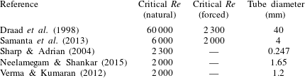
Reference Samanta, Dubief, Holzner, Schäfer, Morozov, Wagner and Hof2013) where, for example, small amounts of fluid are injected in the direction perpendicular to the laminar flow. Table 1 provides a representative summary of transition
 $Re$
for different tube diameters, as reported for the flow of a Newtonian fluid in the references pertinent to the present study. The transition
 $Re$
seems to depend strongly on how the experiment has been carried out and the manner in which inlet disturbances are controlled. For Newtonian fluids, the experiments of Sharp & Adrian (Reference Sharp and Adrian2004) addressed the issue of transition to turbulence in microtubes. They showed that even for tubes with diameters in the range
 ${\sim}250~\unicode[STIX]{x03BC}\text{m}$
, the onset of transition occurred at a Reynolds number of approximately
 $2000$
. No external forcing mechanism was employed in their experiments. In the present experimental work, we carry out experiments similar to Sharp & Adrian (Reference Sharp and Adrian2004) for the flow of polymer solutions in microtubes, and we restrict ourselves to the characterization of natural transition in the flow of Newtonian fluids and viscoelastic polymer solutions.
A representative comparison of transition
 $Re$
for the flow of pure water (Newtonian fluid) through rigid tubes of different diameters as reported by different authors in the literature.

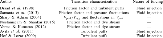
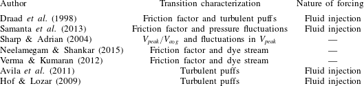
The onset of transition has been characterized by various techniques (table 2). For example, Hof & Lozar (Reference Hof and Lozar2009) and Avila et al. (Reference Avila, Moxey, Lozar, Avila, Barkley and Hof2011) used the survival of localized structures called turbulent puffs to mark the transition. Traditionally, a coloured dye stream is injected into the flow, and the absence of regularity in its motion is taken as a signature of transition. One of the most often used methods is the measurement of pressure drop (i.e. friction factor) in the tube, and examining how this deviates from the expected laminar value. Samanta et al. (Reference Samanta, Dubief, Holzner, Schäfer, Morozov, Wagner and Hof2013) measured pressure fluctuations between two points in the test section of the tube, and located the onset by monitoring the jump in the pressure fluctuations after transition. Similarly, Sharp & Adrian (Reference Sharp and Adrian2004) (for microtubes) and Srinivas & Kumaran (Reference Srinivas and Kumaran2017) (for microchannels) measured the magnitude of velocity fluctuations, and determined the critical Reynolds number for transition based on the sudden jump in the magnitude from its laminar value. Sharp & Adrian (Reference Sharp and Adrian2004) also used the ratio of the maximum velocity at the centre line to the (cross-sectional) average velocity, and the deviation of this ratio from its expected laminar value is taken as a signature of the onset of transition. In the present study, we monitor the ratio of centre-line velocity to average velocity, and also measure the magnitude of velocity fluctuations to identify the onset of transition. We further employ visualization of the dye stream to corroborate the results from micro-PIV measurements.
A summary of characterization methodologies employed to mark the onset of transition and forcing mechanism(s) (if any) employed in the literature.
There has been a large body of literature on the existence of ‘purely elastic’ instabilities in the flow of polymer solutions in geometries with curved streamlines (Larson et al.
Reference Larson, Shaqfeh and Muller1990; Larson Reference Larson1992; Shaqfeh Reference Shaqfeh1996; Groisman & Steinberg Reference Groisman and Steinberg2000; Schiamberg et al.
Reference Schiamberg, Shereda, Hu and Larson2006). The purely elastic instability in such flows can occur at very low
 $Re$
and does not require inertial effects in the fluid for their presence. However, the Weissenberg number
 $Wi=\unicode[STIX]{x1D706}\dot{\unicode[STIX]{x1D6FE}}$
(where
 $\dot{\unicode[STIX]{x1D6FE}}$
is the shear rate in the flow) needs to be sufficiently large to induce such instabilities at low inertia. The instability is driven by the ‘hoop stress’ in the flow of viscoelastic fluids with curved streamlines, and is absent when the flow is rectilinear. In the present study, we focus on the presence of instabilities in tubes wherein the flow is rectilinear in the laminar regime, and we also focus on regimes of
 $Re$
much higher than those considered in the study of purely elastic instabilities.
One of the most dramatic consequences of the addition of very small amounts (
 ${\sim}10~\text{ppm}$
) of polymers to a Newtonian fluid is the drastic reduction (up to 80 % compared to that of the Newtonian solvent) in turbulent frictional losses in flows in pipes and channels (Toms Reference Toms and Burgers1949; Virk et al.
Reference Virk, Merril, Mickly, Smith and Christensen1967; Virk Reference Virk1975; White & Mungal Reference White and Mungal2008; Graham Reference Graham2014), while in the laminar regime there is no significant reduction in the frictional losses compared to the laminar flow of the Newtonian solvent. This implies that there is a strong interaction between the added polymer and the turbulent flow itself. The friction factor data for a Newtonian fluid is often plotted in terms of the Prandtl–Kármán coordinates
 $1/\sqrt{f}$
versus
 $\log (Re\sqrt{f})$
, and for a Newtonian fluid, in the fully turbulent regime the
 $f$
–
 $Re$
relation in this plot will appear as a straight line with a slope
 $2$
, often referred to as the ‘Prandtl–Kármán law’. Upon addition of a few ppm of polymers, the onset of drag reduction in the turbulent flow is marked by the point of departure from the Newtonian Prandtl–Kármán line in this plot. For a given polymer concentration, a dilute solution usually follows the Prandtl–Kármán law up to a certain
 $Re$
, and the data will start to deviate thereafter, signalling the onset of drag reduction. The onset of drag reduction happens at lower
 $Re$
as the concentration of the added polymer is increased. For a fixed concentration of the added polymer, as
 $Re$
is increased, the
 $f$
–
 $Re$
relation for the polymer solution deviates increasingly from the Newtonian relation, and eventually approaches the ‘maximum drag reduction’ (MDR) asymptote. Similarly, for a fixed
 $Re$
, if the concentration of the added polymer is increased, the
 $f$
–
 $Re$
relation for the polymer solution deviates increasingly from the Newtonian relation, and approaches the MDR asymptote. Thus, the drag reduction that can be achieved by the addition of polymers has an upper bound as given by the MDR asymptote. After the onset of transition, in many polymers, the
 $f$
–
 $Re$
curve for a polymer solution follows that of a Newtonian solvent, and the onset of drag reduction begins at a higher
 $Re$
in the Prandtl–Kármán curve for a Newtonian fluid. This behaviour is referred to as ‘Type A’ drag reduction in the literature. However, in some instances, the transition to turbulence is immediately followed by an approach to the MDR asymptote, and this is often referred to as ‘Type B’ drag reduction (Virk Reference Virk1975).
While the onset of the drag reduction is known to be a function of the concentration of the added polymer, the conventional wisdom, however, has been that the transition to turbulence in the flow of the polymer solutions is very similar to that of the Newtonian solvent. The reason behind this paradigm could be because, traditionally, the experimental literature on drag reduction has focused on the role of very small concentrations (
 ${\sim}10~\text{ppm}{-}50~\text{ppm}$
) of the added polymer and tubes of relatively larger diameters, and the onset of transition could be unaffected by the added polymer under such conditions. However, recently Dubief and coworkers (Dubief, Terrapon & Soria Reference Dubief, Terrapon and Soria2013; Terrapon, Dubief & Soria Reference Terrapon, Dubief and Soria2013; Sid, Terrapon & Dubief Reference Sid, Terrapon and Dubief2018) have used simulations to clearly demonstrate the existence of elasto-inertial turbulence for the first time when the elasticity number
 $E=\unicode[STIX]{x1D706}\unicode[STIX]{x1D708}/R^{2}$
is high. These simulations conclusively show that there could be ‘early turbulence’ (at
 $Re$
much lower than
 $2000$
) in the flow of polymer solutions at sufficiently high values of
 $E$
, and subsequently a direct approach to the MDR asymptote, in agreement with the experiments of Samanta et al. (Reference Samanta, Dubief, Holzner, Schäfer, Morozov, Wagner and Hof2013). The elasticity number is directly proportional to the longest relaxation time of the polymer solution
 $\unicode[STIX]{x1D706}$
. Even for concentrations smaller than the overlap concentration, it has been observed (Clasen et al.
Reference Clasen, Plog, Kulicke, Owens, Macosko, Scriven, Verani and McKinley2006; Samanta et al.
Reference Samanta, Dubief, Holzner, Schäfer, Morozov, Wagner and Hof2013) that
 $\unicode[STIX]{x1D706}$
increases weakly with increase in the polymer concentration at suboverlap concentrations. Thus, the reason why early turbulence was not observed in the experimental studies on drag reduction could be attributed to the relatively lower values of elasticity numbers probed in those experiments.
In contrast to the flow of a Newtonian fluid, where
 $Re$
is the only dimensionless parameter for characterizing transition, polymeric flows are characterized in addition by the Weissenberg (
 $Wi$
) number or elasticity number (
 $E$
). Here,
 $Wi$
is the product of shear rate and the longest relaxation time of the polymer solution and the elasticity number is the ratio of
 $Wi$
and
 $Re$
. While the Weissenberg number is a function of flow velocity (or shear rate in the flow), the elasticity number is independent of flow parameters, and is merely a function of the physical properties of the polymer solution and the flow length scale (i.e. radius
 $R$
for flow in tubes). It must, however, be noted that for concentrated polymer solutions, the relaxation time is a function of shear rate and the notion that
 $E$
is a flow-independent parameter is not fully accurate. However, both
 $Wi$
and
 $E$
are strongly dependent on the radius of the tube. Previous experiments performed on different tube diameters have actually probed different elasticity (or Weissenberg) numbers (see table 3).
The experiments of Goldstein et al. (Reference Goldstein, Adrian and Kreid1969) were perhaps the first to suggest the phenomenon of early turbulence upon addition of polymers to a Newtonian solvent. They used laser Doppler anemometry to measure the centre-line velocities in the flow of polyethylene oxide (PEO) solutions (50 ppm by weight) in water. They observed that the ratio of the centre-line to (cross-section)-averaged velocity becomes smaller than the laminar value of
 $2$
at
 $Re$
between
 $1000$
and
 $2000$
. While this deviation could be attributed to shear-thinning of the polymer solution, the authors also measured the root mean square (r.m.s.) of the fluctuating component of the velocity, which showed an increase in its magnitude at
 $Re<2000$
, thus indicating that transition occurs at
 $Re<2000$
for PEO solutions. Very similar conclusions were made in the laser Doppler study of Zakin et al. (Reference Zakin, Ni, Hansen and Reischman1977), who used 50 ppm solutions of both polyethylene oxide (molecular weight
 $5\times 10^{6}~\text{g}~\text{mol}^{-1}$
) and polyacrylamide (molecular weight
 $7\times 10^{6}~\text{g}~\text{mol}^{-1}$
). However, neither of these papers carried out experiments for a range of polymer concentrations to arrive at a systematic trend, nor did they report a more precise range of
 $Re$
where there is an onset of transition. Furthermore, the polymer solution was not systematically characterized in terms of its viscosity and relaxation time in those studies. Without a reasonable knowledge of the relaxation time of the polymer solution, it is difficult to estimate the dimensionless
 $Wi$
or elasticity numbers prevailing in those experiments. Draad et al. (Reference Draad, Kuiken and Nieuwstadt1998) investigated polymer flows through tubes of diameter 40 mm and observed that addition of polymers reduces the natural transition
 $Re$
. The elasticity number
 $E$
was relatively low as compared to that obtained by Srinivas & Kumaran (Reference Srinivas and Kumaran2017) (see table 3) on account of the larger diameter tubes used in their experiments. Bonn et al. (Reference Bonn, Ingremeau, Amarouchene and Kellay2011) found that addition of polymer can lead to low
 $Re$
instabilities similar to elastic turbulence in tube flows. A water–glycerine mixture was used as the test fluid and laser Doppler velocimetry (LDV) was used for analysis. It is to be noted that the solutions used were highly viscous and hence had long relaxation times. However, instabilities were reported only for a perturbed inlet wherein the inlet had a lower diameter than the tube itself, thereby creating a ‘jet-like’ inlet arrangement. Further, salt was added in the preparation of the solution, which can change the conformation of the polymer chain in the solution (Draad et al.
Reference Draad, Kuiken and Nieuwstadt1998). Pan et al. (Reference Pan, Morozov, Wagner and Arratia2013) considered flow in rectangular channels and showed that transition can occur at very low
 $Re$
even for straight geometries, which is contrary to the belief that such instabilities can only be induced in curvilinear geometries. They showed that even for geometries in which the flow occurs with straight streamlines, early transition can appear because of the elastic nature of the fluid. However, such instabilities were only sustained with the help of inlet disturbances, and hence cannot be considered as natural transition. It was observed that if the inlet disturbance is removed, the flow remains stable for all values of
 $Wi$
used in the study. Furthermore, the work of Pan et al. (Reference Pan, Morozov, Wagner and Arratia2013) focused on rectangular channels, which can exhibit different flow behaviour as compared to cylindrical tubes.
A comparison of the transition
 $Re$
, polymer concentration
 $C_{p}$
, Weissenberg (
 $Wi$
) and elasticity number (
 $E$
) as inferred from earlier studies in the literature. All these results are for natural transition (i.e. no forcing mechanism employed). Here,
 $\unicode[STIX]{x1D6FD}$
is the ratio of solvent viscosity and solution viscosity.

Samanta et al. (Reference Samanta, Dubief, Holzner, Schäfer, Morozov, Wagner and Hof2013) studied the onset of transition in polyacrylamide solutions in rigid tubes of diameters ranging from 4 mm to 10 mm. For smaller concentrations (up to 175 ppm), they used the survival probability of localized structures called ‘turbulent puffs’ to mark the transition. For larger concentrations, the increase in the normalized pressure fluctuations was used for characterizing the transition. It was concluded that at higher polymer concentrations, the transition to turbulence is different compared to transition to turbulence in Newtonian fluids, and the transition
 $Re$
could be as low as
 $800$
for the flow of polymer solutions at higher concentrations (
 ${\sim}500~\text{ppm}$
). Such a transition was referred to as ‘elasto-inertial turbulence’ (Dubief et al.
Reference Dubief, Terrapon and Soria2013; Samanta et al.
Reference Samanta, Dubief, Holzner, Schäfer, Morozov, Wagner and Hof2013), since it is believed that both elasticity of the polymer solution and fluid inertial effects are important in destabilizing the flow. Furthermore, it was found that the onset of transition scaled with the shear rate of the flow and not with Reynolds number. However, there are a few issues in the observations of Samanta et al. (Reference Samanta, Dubief, Holzner, Schäfer, Morozov, Wagner and Hof2013) which require further investigation. For lower concentrations (up to 175 ppm), the transition as marked by the survival of turbulent puffs agreed well with that from friction factor data and with the (normalized) pressure fluctuation data. However, for the 500 ppm solution (figures 2b and 2d of their paper), while the pressure fluctuations show an increase at
 $Re\sim 800$
, the corresponding friction factor data do not show any deviation from the laminar line at
 $Re\sim 800$
, but start to deviate only at
 $Re\sim 2000$
. It might be expected that the friction factor should start deviating from its laminar value once the instability has been initiated, but this is not borne out by the data of Samanta et al. (Reference Samanta, Dubief, Holzner, Schäfer, Morozov, Wagner and Hof2013). For polymer solutions, it could be possible that the
 $f$
versus
 $Re$
curve deviates slowly from the laminar line, unlike in a Newtonian fluid, but this could not be clearly established from their friction factor data. This also provides the motivation for the present study, where we mark the transition using micro-PIV characterization and further confirm it by using dye-stream visualization. With the exception of the experiments of Samanta et al. (Reference Samanta, Dubief, Holzner, Schäfer, Morozov, Wagner and Hof2013), there have been very few studies on the flow of polymer solutions through microtubes which probe the high shear rates prevailing at relatively low velocities, thus leading to regimes of higher
 $Wi$
or
 $E$
. Recently, Srinivas & Kumaran (Reference Srinivas and Kumaran2017) showed that when small amounts of polymer are added to water, the transition is initiated at a lower Reynolds number (
 ${\sim}400$
) for flow through a rectangular channel with smallest dimension in the range of
 $100~\unicode[STIX]{x03BC}\text{m}$
. Thus, the experiments of Samanta et al. (Reference Samanta, Dubief, Holzner, Schäfer, Morozov, Wagner and Hof2013) for tube flows and the experiments of Srinivas & Kumaran (Reference Srinivas and Kumaran2017) for rectangular channel flows show that flow of polymer solutions can exhibit qualitatively new instabilities absent in Newtonian fluids.
Bodiguel et al. (Reference Bodiguel, Beaumont, Machado, Martinie, Kellay and Colin2015) reported instabilities in the flow of highly shear-thinning concentrated polymer solutions in rectangular microchannels (where the smallest cross-flow direction is in the range
 $150~\unicode[STIX]{x03BC}\text{m}{-}170~\unicode[STIX]{x03BC}\text{m}$
). The Reynolds numbers prevalent in their experiments are less than
 $0.02$
, thus placing their experiments in a very different parametric regime compared to the present study. The experiments of Poole (Reference Poole2016) and Wen et al. (Reference Wen, Poole, Willis and Dennis2017) also examined the flow of highly shear-thinning concentrated polymer solutions in tubes and channels, but the radii of the tubes are
 $O(10)~\text{cm}$
, and the polymer concentrations are approximately 50–100 times greater than the ones considered in the present study. Thus, while the observations of Bodiguel et al. (Reference Bodiguel, Beaumont, Machado, Martinie, Kellay and Colin2015) and Poole (Reference Poole2016) also reveal qualitatively new instabilities, the polymer solutions considered in those studies are much more concentrated, and the Reynolds numbers much lower compared to the conditions considered in the present study.
The aim of the present study is to explore the modification of transition to turbulence by the addition of polymers to water in tubes using the micro-PIV and dye-stream visualization methods. In order to establish the robustness of the phenomena observed, we carry out experiments involving the flow of two different polymers (viz., polyacrylamide and polyethylene oxide) of differing molecular weights in tubes of two different diameters:
 ${\sim}390~\unicode[STIX]{x03BC}\text{m}$
and
 $470~\unicode[STIX]{x03BC}\text{m}$
. We further demonstrate the possibility of collapse of various experimental data for the transition
 $Re$
when plotted in terms of relevant dimensionless parameters. The rest of this paper is organized as follows. Section 2 describes the experimental protocol which has been employed in preparing the microtubes, its characterization and preparation of the polymer solutions and their characterization. Section 3 provides the detailed micro-PIV analysis for flow of a pure Newtonian solvent, polyacrylamide and polyethylene oxide solutions through microtubes. In § 4 we provide a comparative discussion of our results in the context of earlier experimental literature. Section 5 provides the main conclusions of the present study.
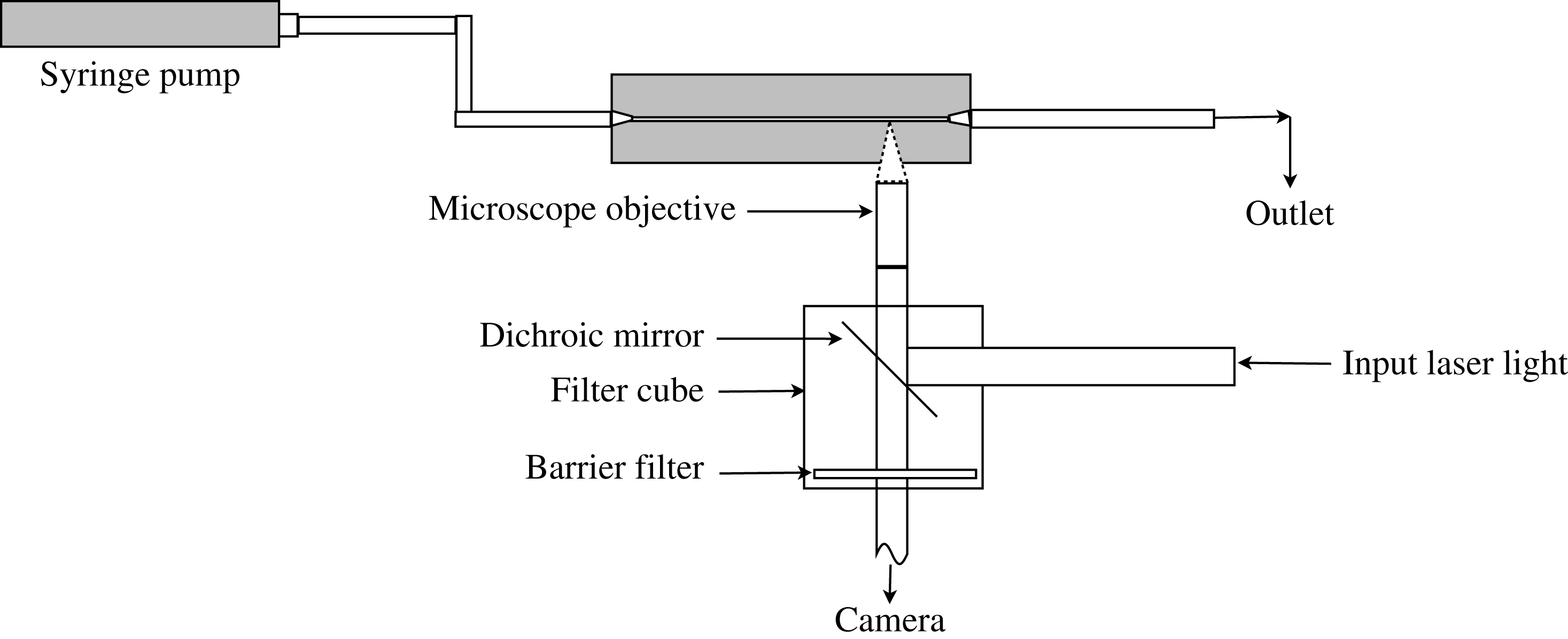
Schematic of the experimental set-up used in our micro-PIV measurements.

2 Experimental set-up and procedure
The experimental configuration used to perform the micro-PIV measurements is shown in figure 1. Pressure-driven flow is carried out through microtubes with the help of a syringe pump (Harvard Apparatus). A pulsed laser (Quantel, pulse frequency 15 Hz, power
 $15~\text{mJ}~\text{pulse}^{-1}$
, wavelength 532 nm) is used to visualize the fluorescent polystyrene seed particles and a CCD camera (Powerview, TSI, f-number f/2) of resolution
 $3320~\text{pixels}\times 2496~\text{pixels}$
(8.3 megapixels) is used to capture images. A synchronizer is used to synchronize the camera and the laser while obtaining images. The time between the pulses is calculated on the basis of the peak velocity corresponding to each flow rate, and varies in the range of 220 ns–2000 ns, depending on the flow rate. It is important to note that the time between pulses is much lower in micro-PIV studies as compared to macroscale PIV because of the magnification of the image. We used a 10
 $\times$
objective for magnification, and hence we rescale the time between pulses accordingly. All the experiments are performed at
 $25~^{\circ }\text{C}$
, which is maintained with the help of air conditioners. The room is kept dark while capturing the images from the camera. The images obtained are processed using Insight 4G software (TSI, Shoreview).
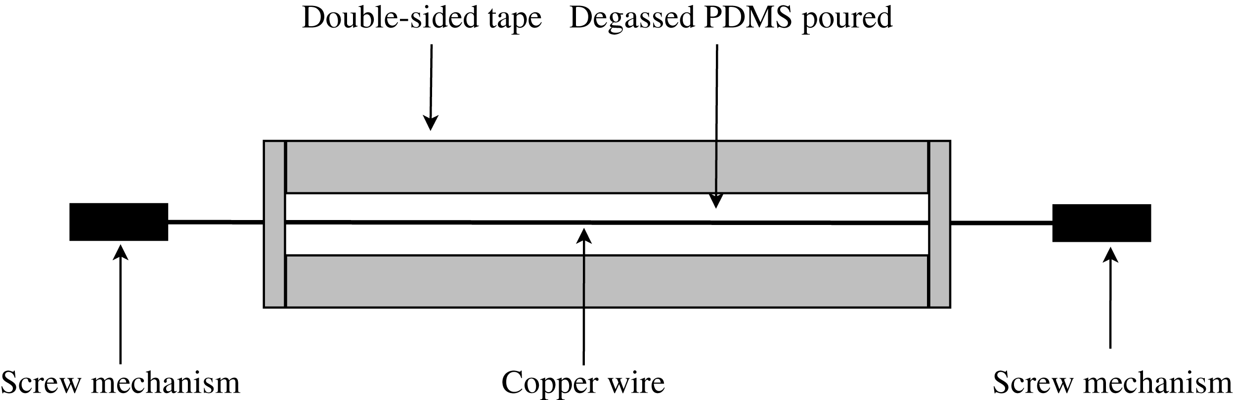
Fabrication process for microtubes. PDMS elastomers of very high shear modulus (
 ${\sim}0.35~\text{MPa}$
) were used for preparing rigid tubes.

2.1 Fabrication of microtubes
Tubes of diameters
 $390~\unicode[STIX]{x03BC}\text{m}$
and
 $470~\unicode[STIX]{x03BC}\text{m}$
are prepared in rectangular polydimethylsiloxane (PDMS; Sylguard 184 procured from Dow Corning) blocks. Two copper wires of different diameters (Alcoa Prime) are used as a template which is held straight using a screw mechanism and double-sided tape. A rectangular well (figure 2) is created using double-sided tape and the wire is held straight in the rectangular well using the screw mechanism. The well is prepared in a manner similar to the protocol of Neelamegam & Shankar (Reference Neelamegam and Shankar2015), except that a copper wire is used here as a template. The PDMS kit consists of an elastomer base and a curing agent. The required amount of curing agent is added to the elastomeric base, which is then mixed thoroughly. The liquid mixture is then degassed to remove air bubbles, after which it is slowly poured into the well. The well containing the PDMS mixture is now cured in a preheated oven at
 $80~^{\circ }\text{C}$
for 4 h. After curing, the PDMS block is kept in toluene solution for 2–3 h while swelling. The copper wire is slowly removed after swelling and thus a tubular bore is created in the PDMS block. De-swelling is carried out at low temperatures to avoid crack formation in the tube. The choice of PDMS for tube fabrication is due to its lower refractive index value (
 ${\sim}1.41$
) as compared to glass (
 ${\sim}1.5$
) or fused silica (
 ${\sim}1.46$
). Since our test fluid is water, and hence the polymer solution has a refractive index close to 1.33, using PDMS will be more effective in reducing optical distortion in our micro-PIV experiments. Furthermore, the transparent nature of the PDMS block allows for dye-stream visualization in the flow.
2.2 Preparation of polymer solutions
The polymer solution is prepared by mixing small amounts of high-molecular-weight polymers in deionized water. We use two different polymers in our study: polyacrylamide (
 $\text{MW}=5\times 10^{6}~\text{g}~\text{mol}^{-1}$
) and polyethylene oxide (
 $\text{MW}=8\times 10^{6}~\text{g}~\text{mol}^{-1}$
), both procured from Sigma-Aldrich. The required amount of polymer is added to deionized water and the resultant liquid is slowly mixed using a magnetic stirrer. The polymer solution thus prepared is used in our flow experiments within three days (for polyacrylamide) or 8 h (for polyethylene oxide) of preparation, since polyethylene oxide solutions are found to be more prone to ageing, as discussed later. The solution used is characterized before and after the experiments to check for the effect of ageing with time. The properties of the fluid do not change during the time scale of the experiments, which is approximately 2–3 h. Experiments are always performed using freshly prepared polymer solutions to avoid any ageing effects. Measurement of viscosity is done using a TA DHR-3 rheometer with the help of a concentric cylinder geometry.
2.3 Characterization of PDMS tubes
The PDMS mixture used for tube fabrication is also prepared in rectangular slabs of 4 mm thickness for characterization. Small-amplitude oscillatory experiments are performed on these slabs in order to measure the frequency-dependent shear modulus. The shear moduli of the gels prepared are more than
 $10^{5}~\text{Pa}$
, and hence can be considered as rigid, as has been extensively documented by the earlier studies of Verma & Kumaran (Reference Verma and Kumaran2012). In this study, we also demonstrate that the transition of a Newtonian fluid in such a tube happens at
 $Re\sim 2000$
, similar to rigid materials such as glass or steel. The diameter of the prepared tube is measured at different axial locations to check for uniformity of the tube dimensions using the 10
 $\times$
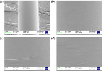
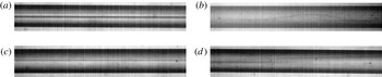
objective of a microscope. A microscopic scale is used for calibration of the microscope. The deviation of the diameter of the fabricated tubes is less than 1 % within the tube. In order to check the extent of roughness in the inner surface of the prepared tube, we carried out imaging using scanning electron microscopy (SEM). To obtain the images, we cut open the PDMS block in which the tube is present such that the hollow cylindrical surface of the tube is exposed. The SEM images of the inner surface of the tubes are shown in figure 3. Magnifications used in the imaging are similar to Verma & Kumaran (Reference Verma and Kumaran2012). The SEM images of our tubes suggest that the roughness present in the fabricated tubes is negligible.
SEM images of microtubes at different magnifications, i.e (a) 400
 $\times$
, (b) 1500
 $\times$
, (c) 2000
 $\times$
and (d) 3000
 $\times$
, to demonstrate the smoothness of the inner surface of the tubes fabricated.

2.4 Characterization of polymer solution
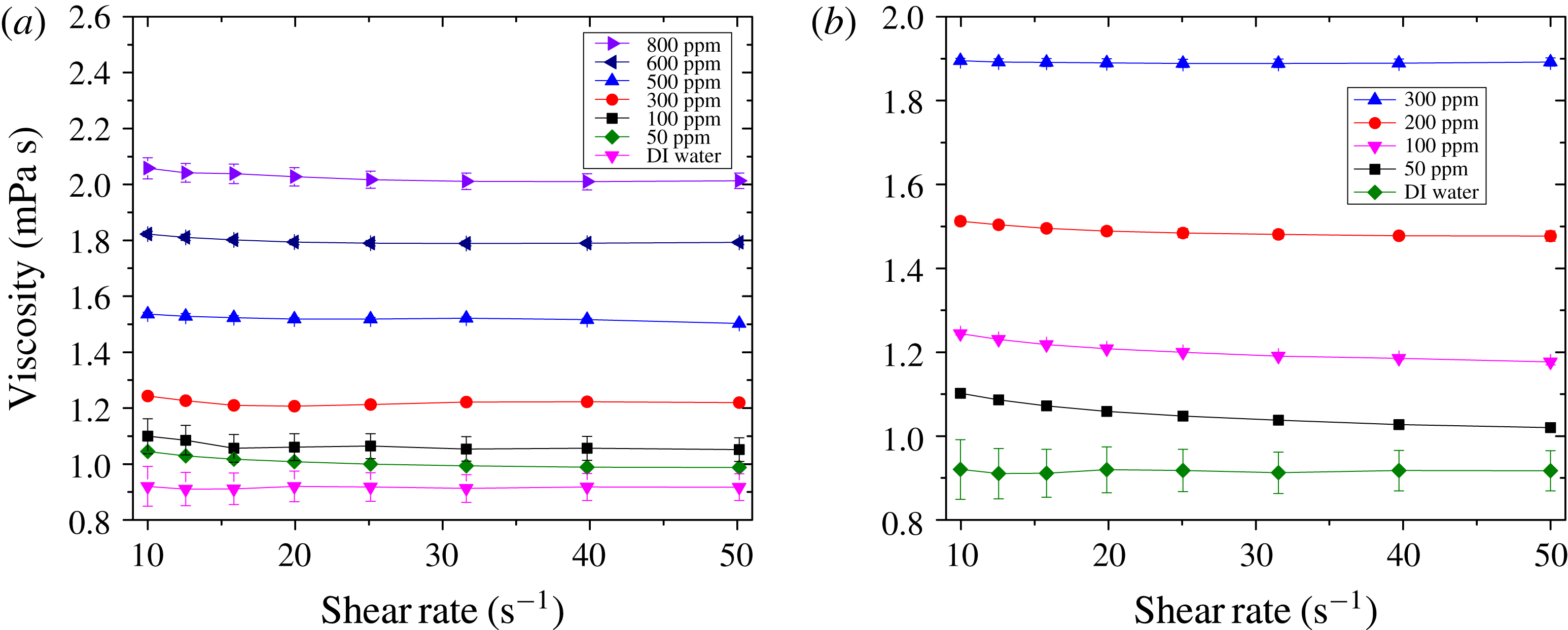
The viscosity of the polymer solutions is measured using a TA DHR-3 rheometer with the help of a concentric cylinder geometry. The viscosity is measured with shear rates in the range
 $10~\text{s}^{-1}{-}50~\text{s}^{-1}$
(figure 4). The results show that the shear-rate dependence of the viscosity is negligible in both the solutions in the observed range of shear rates. The zero-shear viscosities of the various solutions used in our experiments are summarized in table 4. However, the nominal shear rates in the flow experiments carried out later in this work are very high, but it is not possible to use the rheometer to measure the viscosity at such high shear rates encountered in the flow experiments. The effect of ageing is studied on both polyacrylamide solution and polyethylene oxide (PEO) solution by observing the change in viscosity with time. It is observed that the PEO solution is more prone to ageing. Hence viscosity is always measured before and after flow experiments to ensure that the solution had not aged sufficiently during the flow experiments. However, the viscosity of polyacrylamide solution does not change appreciably over the time scales for which such studies are performed for the PEO solution. Hence it was ensured that experiments are performed within 3 h of preparation of the PEO solution.
Viscosity as a function of shear rate for (a) polyacrylamide solution (
 $\text{molecular weight}=5\times 10^{6}$
) and (b) polyethylene oxide (
 $\text{molecular weight}=8\times 10^{6}$
).

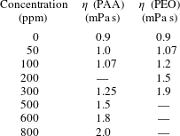
A comparison of solution viscosity
 $\unicode[STIX]{x1D702}$
of the two polymer solutions used in our study at different concentrations. PAA stands for polyacrylamide (
 $\text{MW}=5\times 10^{6}$
) and PEO for polyethylene oxide (
 $\text{MW}=8\times 10^{6}$
).

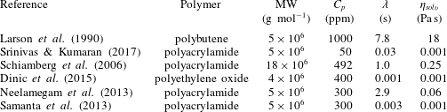
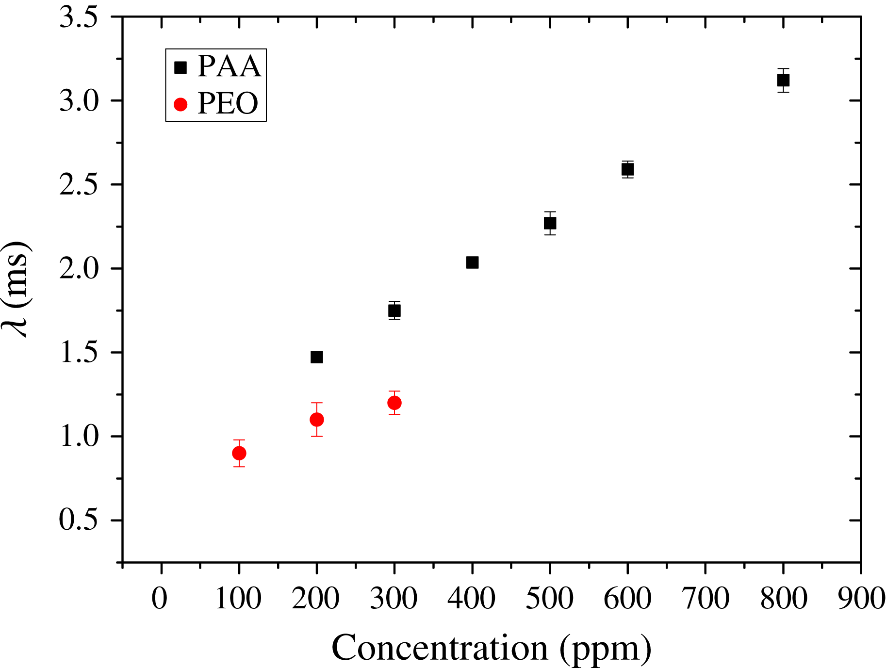
The characterization of relaxation time of a dilute polymer solution can be done in a variety of ways, and often the results from different methods do not agree accurately with each other (table 5), as has been recently noted by Srinivas & Kumaran (Reference Srinivas and Kumaran2017). In the literature, Larson et al. (Reference Larson, Shaqfeh and Muller1990) and Schiamberg et al. (Reference Schiamberg, Shereda, Hu and Larson2006) use the first normal stress coefficient to estimate relaxation time, and report relaxation times of the order of a few seconds. Larson et al. (Reference Larson, Shaqfeh and Muller1990) used low-molecular-weight polybutene and Schiamberg et al. (Reference Schiamberg, Shereda, Hu and Larson2006) used sucrose to increase viscosity of the solution. Recently, Dinic et al. (Reference Dinic, Zhang, Jimenez and Sharma2015) use the capillary breakup (‘CaBeR’) technique for calculating relaxation time. They estimate the relaxation time on the order of 1 ms for PEO solutions. Samanta et al. (Reference Samanta, Dubief, Holzner, Schäfer, Morozov, Wagner and Hof2013) also use the ‘CaBeR’ technique for measurement of relaxation time. Neelamegam, Shankar & Das (Reference Neelamegam, Shankar and Das2013) use the single-mode Maxwell model for estimation of relaxation time, where the solvent viscosity is increased by the addition of sucrose to water. However, small-amplitude oscillatory experiments do not give satisfactory data for the low-viscosity solvent (i.e. water) used in our study.
A comparison of relaxation times as estimated by different authors;
 $C_{p}$
is the polymer concentration.

To overcome this difficulty, we increased the viscosity of the solvent by adding glycerine to water, thus increasing the possibility of obtaining reliable results from small-amplitude oscillatory experiments. One consequence that must be avoided due to the addition of glycerine is that the solvent quality should not be modified significantly. This was noted in the experiments of Fang, Brown & Hvidt (Reference Fang, Brown and Hvidt1992), who measured the radius of gyration of polyacrylamide in glycerol solutions at different glycerine concentrations and showed that there is only a very modest change in the radius of gyration as the glycerine concentration is changed. In our experiments, the polyacrylamide solution was prepared by dissolving polymer in
 $90\,\%$
glycerine solution. Small-strain oscillatory experiments are performed on the prepared solution with increased solvent viscosity. For a truly dilute solution of polymers, the Zimm (or Rouse) relaxation time is directly proportional to solvent viscosity (Doi & Edwards Reference Doi and Edwards1988), and hence in the dilute limit it is possible to measure the relaxation time at a higher solvent viscosity and then scale it appropriately to lower solvent viscosities as desired. In the truly dilute limit, the relaxation time is independent of polymer concentration. Using the reported radius of gyration of
 $0.184~\unicode[STIX]{x03BC}\text{m}$
for polyacrylamide of molecular weight
 ${\sim}5\times 10^{6}$
(Kulicke, Kniewske & Klein Reference Kulicke, Kniewske and Klein1982), and a solvent viscosity of 0.001 Pa s, we obtain the Zimm relaxation time for our system as
 $1.4\times 10^{-3}~\text{s}$
. The overlap concentration for our polymer solution is obtained using
 $c^{\ast }=0.77/[\unicode[STIX]{x1D702}]$
, where
 $[\unicode[STIX]{x1D702}]$
is the intrinsic viscosity of our solution and
 $c^{\ast }\sim 600~\text{ppm}$
for the polyacrylamide solution used.
The concentrations used in our transition experiments are in the range 50 ppm–800 ppm, thus placing them in the dilute regime or the cross-over to the semidilute regime. Although some of our concentrations are in the onset of cross-over to the semidilute regime, we nonetheless scale the relaxation time (from glycerol solutions to that of pure water) assuming that it is directly proportional to solvent viscosity, as one would expect for a truly dilute system. Figure 5 shows the relaxation time obtained using the glycerine–water–polymer mixture after it is scaled down according to the decrease in solvent viscosity for pure water. The results thus obtained are in fairly good agreement with the results of Samanta et al. (Reference Samanta, Dubief, Holzner, Schäfer, Morozov, Wagner and Hof2013), who used the ‘CaBeR’ technique for estimating the relaxation time. For polyacrylamide solutions, however, we were not able to reliably estimate the relaxation time for concentrations below 100 ppm. For 200 ppm, the experimentally inferred relaxation time already approaches the estimated Zimm relaxation time (valid for the truly dilute regime), and hence we use the Zimm relaxation time for
 $c<200~\text{ppm}$
. The weak concentration dependence of relaxation time at suboverlap concentrations was also reported in the earlier work of Clasen et al. (Reference Clasen, Plog, Kulicke, Owens, Macosko, Scriven, Verani and McKinley2006) and Samanta et al. (Reference Samanta, Dubief, Holzner, Schäfer, Morozov, Wagner and Hof2013).
Although this protocol worked for polyacrylamide solutions, it was observed that polyethylene oxide was not soluble in glycerol solutions. It was shown by Ebagninin, Benchabane & Bekkour (Reference Ebagninin, Benchabane and Bekkour2009) that low-molecular-weight polyethylene oxide (MW
 $1\times 10^{5}$
) behaves as a Newtonian fluid even at concentrations up to 20 % by weight. Since polyethylene oxide (MW
 $8\times 10^{6}$
) is soluble in polyethylene oxide (MW
 $1\times 10^{5}$
), we were able to increase the solvent viscosity of the polymer solution prepared. We use low-molecular-weight polyethylene oxide (MW
 $1\times 10^{5}$
) to obtain a mixture of PEO (MW
 $1\times 10^{5}$
), PEO (MW
 $8\times 10^{6}$
) and water. This gives us satisfactory oscillatory shear data that enable us to estimate the relaxation time using a single-mode Maxwell fit. Our relaxation time data obtained with this procedure are in close agreement with the relaxation time obtained using the ‘CaBeR’ technique by Dinic et al. (Reference Dinic, Zhang, Jimenez and Sharma2015). However, we were not able to obtain the relaxation time reliably for the lowest polymer concentration used in our study (50 ppm). For such low concentrations, it is reasonable to assume that the relaxation time is independent of concentration, and hence we used the relaxation time obtained using
 $c=100~\text{ppm}$
for
 $c<100~\text{ppm}$
.
Relaxation time of polyacrylamide (molecular weight:
 $5\times 10^{6}$
) and polyethylene oxide (molecular weight:
 $8\times 10^{6}$
) solutions obtained by fitting oscillatory data into a single-mode Maxwell model. The oscillatory experiments were carried out with solvents of a much higher viscosity than water (which ensures that the data from the oscillatory experiments are reliable), and the results for the relaxation time are rescaled for water as the solvent.

2.5 Experimental protocol
The polymeric solution is prepared for micro-PIV analysis by adding fluorescent polystyrene particles (diameter
 $3.2~\unicode[STIX]{x03BC}\text{m}$
) procured from Thermo Fisher Scientific, which are already dispersed in deionized water. We estimated the Stokes number to be
 $O(0.01)$
in our experiments, and hence the seed particles are expected to follow the fluid streamlines faithfully. Further, the Péclet numbers based on the seed particle self-diffusivity are very large, indicating that Brownian motion is negligible. While preparing the polymer solution for PIV, we first prepare a solution of seed particles in pure deionized water. This seed particle solution is sonicated for 60 s to break any agglomeration of particles. This is then added to the polymer solution to obtain the desired polymer concentration. It is to be noted that increasing seed particle concentration may increase the number of vectors obtained, but it also increases the number of out-of-plane particles. This increases noise in the experiments, and hence we use an optimum number of particles to obtain the velocity vectors. The concentration of seed particles is increased in a stepwise manner to arrive at the optimum concentration at which we get maximum number of acceptable velocity vectors. A cross-correlation method is used for processing images with an interrogation window of
 $64~\text{pixels}\times 64~\text{pixels}$
for inferring seed particle displacement. For micro-PIV, it is observed that volume illumination occurs because of the small diameter of the tube used. This causes visibility of low-intensity out-of-plane seed particles as well. This may result in noise during image processing. The images are run through a filter algorithm to remove the low-intensity out-of-plane seed particles. The PIV measurements are taken at a distance of 120 diameters from the entry of the flow in the microtube, which enables us to neglect any entrance effects.
Since the tubes considered in the present experiments are cast inside a rectangular PDMS block, curvature effects are minimal. However, the refractive indices of water (
 ${\sim}1.3$
) and the surrounding solid PDMS (
 ${\sim}1.4$
) are slightly different, and hence the PIV measurements are somewhat prone to optical distortion. However, optical distortion is minimal at the centre of the tube, and hence we extract all our data from the centre line of the tube in a very similar way to the experiments of Sharp & Adrian (Reference Sharp and Adrian2004) for flow of Newtonian fluids. Optical distortion is significant as we move away from the centre of the tube, as manifested in the experimentally obtained velocity profiles. The mismatch between the theoretical laminar velocity profile and the experimental velocity profile becomes more prominent as we move away from the centre of the tube. For Newtonian fluids under laminar conditions, the error between the measured and theoretical velocities is approximately
 $2\,\%$
near the centre and approximately
 $8\,\%$
near the tube wall.
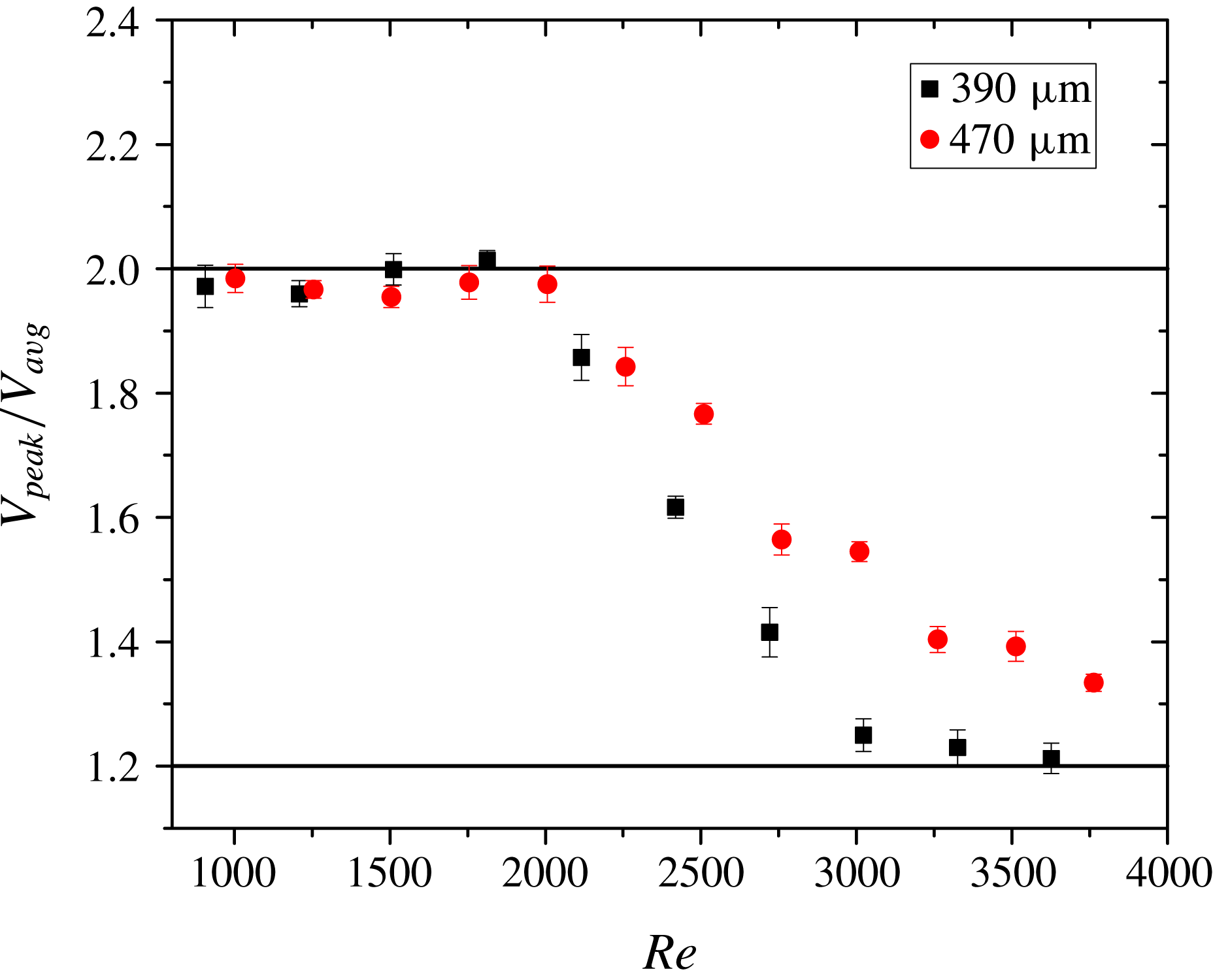
Ratio of the time-averaged peak velocity to cross-section average velocity in Newtonian fluid through a rigid microtube. Transition is detected by deviation of the ratio of peak velocity to average velocity from the laminar value of 2. Tubes of two different diameters are used in our experiments. Transition occurs at approximately the same
 $Re$
for both the tubes, which is consistent with the established result that transition occurs at approximately
 $Re\sim 2000$
for a Newtonian fluid.

Two types of image processing methods are used. In the first method, multiple images are averaged over time to obtain the time-averaged velocity profile. The centre-line time-averaged velocity is divided by the (cross-sectional) average velocity to facilitate comparison with theoretically expected laminar flow values. The cross-section average velocity in the flow is calculated from the flow rate of the syringe pump, and this is further verified by collecting the liquid at the outlet of the flow. The ratio of the centre-line to cross-section average velocity should be ideally equal to 2 for laminar flow of a Newtonian fluid through a rigid tube. The value tends to reach 1.2 for fully turbulent flows and is between 1.2 and 2 in the transition regime. In the second method, images are processed separately at every time instant. The centre-line velocity at each time instant is calculated by taking the average of velocities at the centre line of the tube at different axial locations. The centre-line velocity thus obtained at each time instant is averaged over time. The r.m.s. velocity fluctuations are normalized by the time-averaged centre-line velocity.
We performed three sets of experiments for each flow rate used in our experiments. The data is presented with error bars which represent deviation in our experiments from the average over different experimental runs.
3 Onset of transition in polymer solutions
First, we characterize the onset of transition in the flow of a Newtonian fluid through microtubes. This helps in benchmarking our experimental protocol to characterize laminar–turbulent transition. We verify this phenomenon for deionized water (figure 6) and then use this protocol to infer transition in the flow of polymer solutions. In the following discussion,
 $V_{avg}$
is the cross-section average velocity as inferred from measurement of volumetric flow rates in each experiment, and this is used to non-dimensionalize the peak velocity in the velocity profiles, as shown in figure 6. Time-averaged velocity profiles (i.e. velocity at different radial locations in the tube) are obtained at different
 $Re$
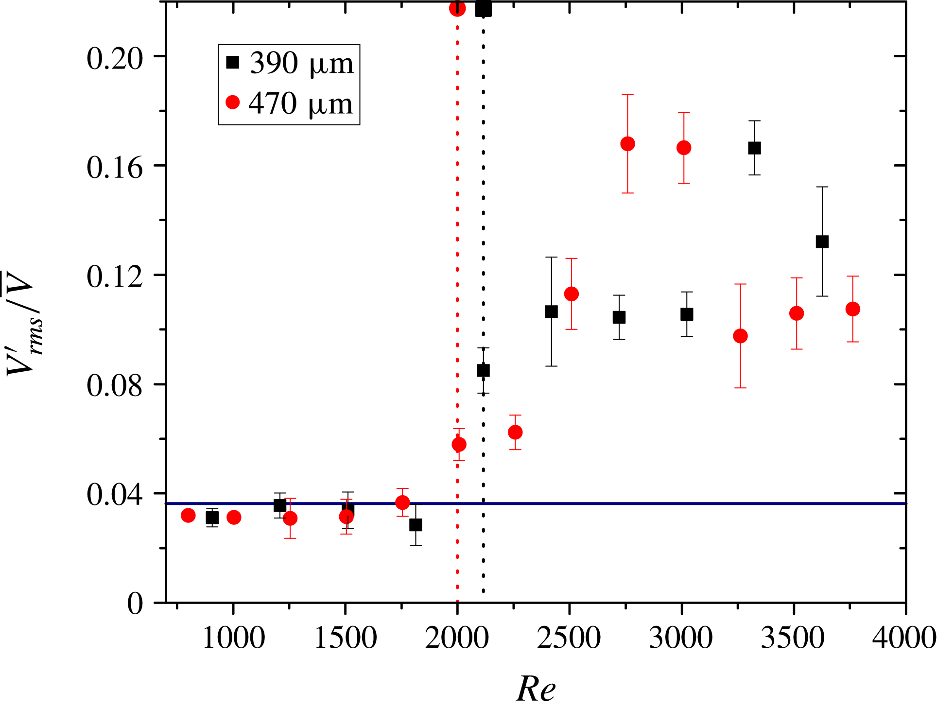
. We observe that the velocity profile deviates from the parabolic profile in the transition regime and becomes more plug-like in the fully turbulent regime. Transition is also inferred from a jump in normalized r.m.s. centre-line velocity fluctuations (figure 7) with increasing
 $Re$
. Here, and in what follows,
 $Re\equiv DV_{avg}\unicode[STIX]{x1D70C}/\unicode[STIX]{x1D702}$
, where
 $\unicode[STIX]{x1D702}$
is the viscosity of the solution and
 $D=2R$
is the tube diameter. In this figure, and in subsequent figures showing r.m.s. velocity fluctuations, the r.m.s. velocity value is non-dimensionalized with the time-averaged centre-line velocity from the PIV measurements (denoted by
 $\bar{V}$
). We have further verified that even if the r.m.s. data are taken at a different radial location away from the centre of the tube, there is still a jump in the r.m.s. of velocity fluctuations. As expected, the transition
 $Re$
is independent of the tube diameter for Newtonian fluids, and is close to the well-established value of
 $2000$
in our experiments.
Variation of magnitude of velocity fluctuations with
 $Re$
in Newtonian fluid flow through microtubes. Two different diameters are used in our experiments. Transition occurs at
 $Re$
of approximately 2000, which is consistent with the time-average velocity results. Horizontal line is an indication of the magnitude of fluctuations in the laminar regime. The vertical dotted line is an indicator of the transition
 $Re$
.

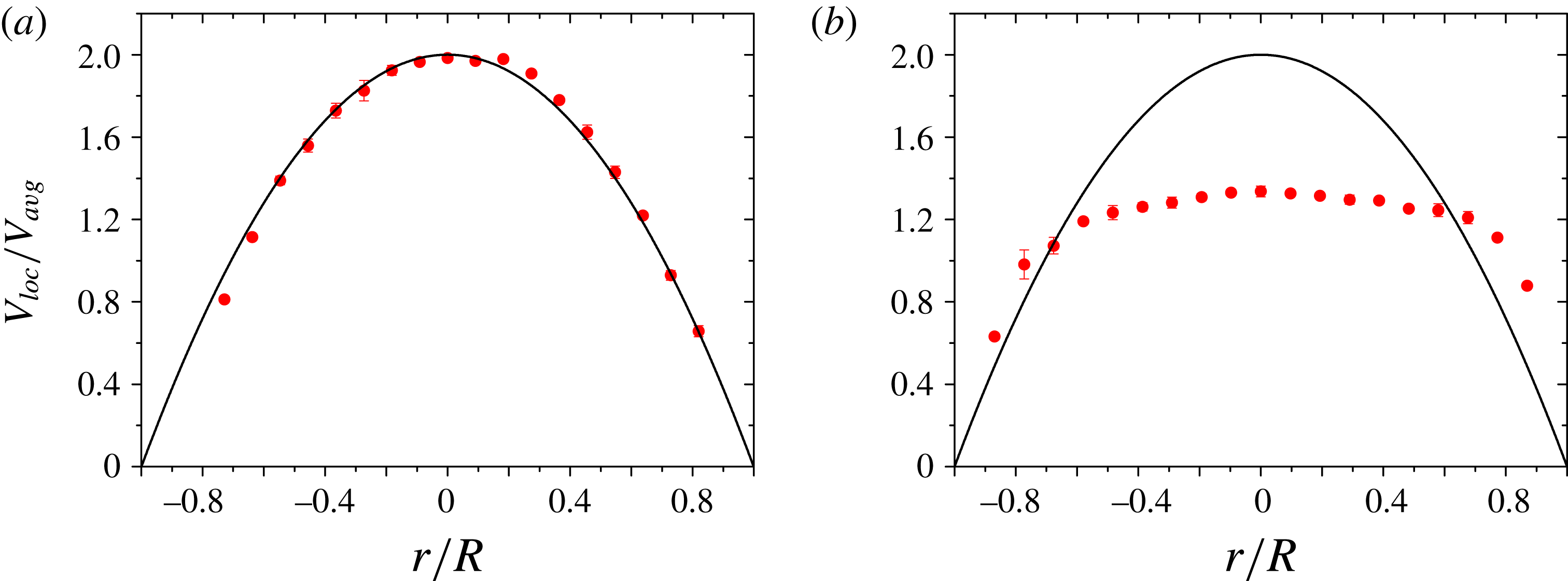
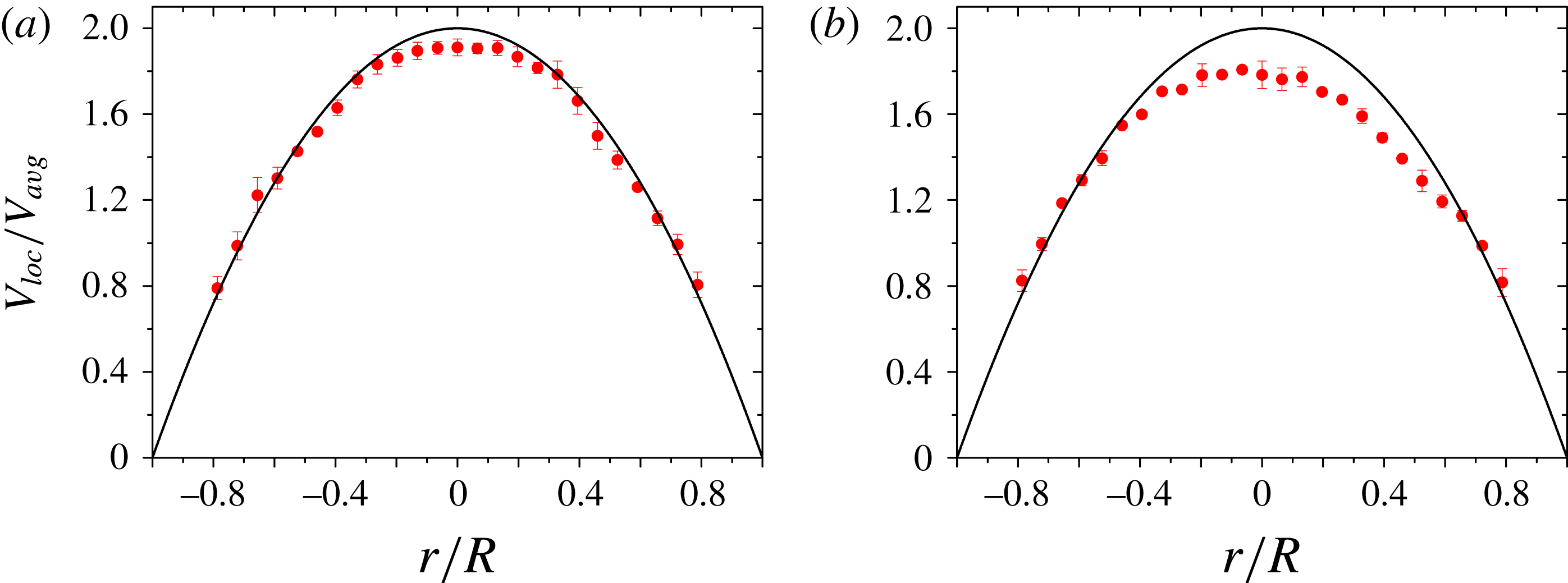
Scaled velocity profile comparison for laminar and transition regime of a Newtonian fluid through a rigid microtube of diameter
 $470~\unicode[STIX]{x03BC}\text{m}$
. Here, and in what follows,
 $V_{loc}$
is the local fluid velocity and
 $r$
is the coordinate in the direction perpendicular to the flow;
 $r=0$
denotes the tube centre. (a) Laminar flow at
 $Re=1000$
and (b) flow after transition at
 $Re=3750$
. The continuous line represents the theoretical velocity profile for a Newtonian fluid in the laminar regime and symbols represent the experimentally obtained velocity profile.

A deviation in the centre-line velocity from its expected laminar value is an indicator of onset of transition. Srinivas & Kumaran (Reference Srinivas and Kumaran2015) show that post-transition flows in channels have a more plug-like velocity profile as compared to the laminar state. The velocity profile in the case of a turbulent flow becomes more plug-like, whereas a laminar flow has a parabolic flow profile (figure 8). We found that it is difficult to obtain the velocity accurately very near the tube wall, as the refractive indices of the fluid and the surrounding PDMS block are somewhat different. However, the velocity profile very clearly indicates plug-like behaviour in the post-transition regime. The earlier works of Goldstein et al. (Reference Goldstein, Adrian and Kreid1969) and Patel & Head (Reference Patel and Head1969) used the ratio of peak to average velocity to characterize transition in tubes with diameter 10 mm. More recently, Sharp & Adrian (Reference Sharp and Adrian2004) carried out micro-PIV measurements without refractive-index matching in a tube of diameter
 $247~\unicode[STIX]{x03BC}\text{m}$
. The tube diameters used in our study are comparable to those of Sharp & Adrian (Reference Sharp and Adrian2004) and the results obtained for the transition Reynolds number for a Newtonian fluid in this study match quite closely with the results of Sharp & Adrian (Reference Sharp and Adrian2004).
We next carried out flow experiments with polymer solutions, and the onset of transition to turbulence for polymer flows is characterized using the protocol used for Newtonian flows discussed above. All the flow experiments are performed with fresh polymer solutions and the experiments are completed within three hours after the preparation of the fresh solution. We discuss the results obtained for solutions of polyacrylamide in water first, and then proceed to discuss the results for polyethylene oxide solutions.
3.1 Onset of transition in the flow of polyacrylamide solutions
Figure 9 shows the variation of the ratio
 $V_{peak}/V_{avg}$
with
 $Re$
for flow in tubes of diameter
 $390~\unicode[STIX]{x03BC}\text{m}$
and
 $470~\unicode[STIX]{x03BC}\text{m}$
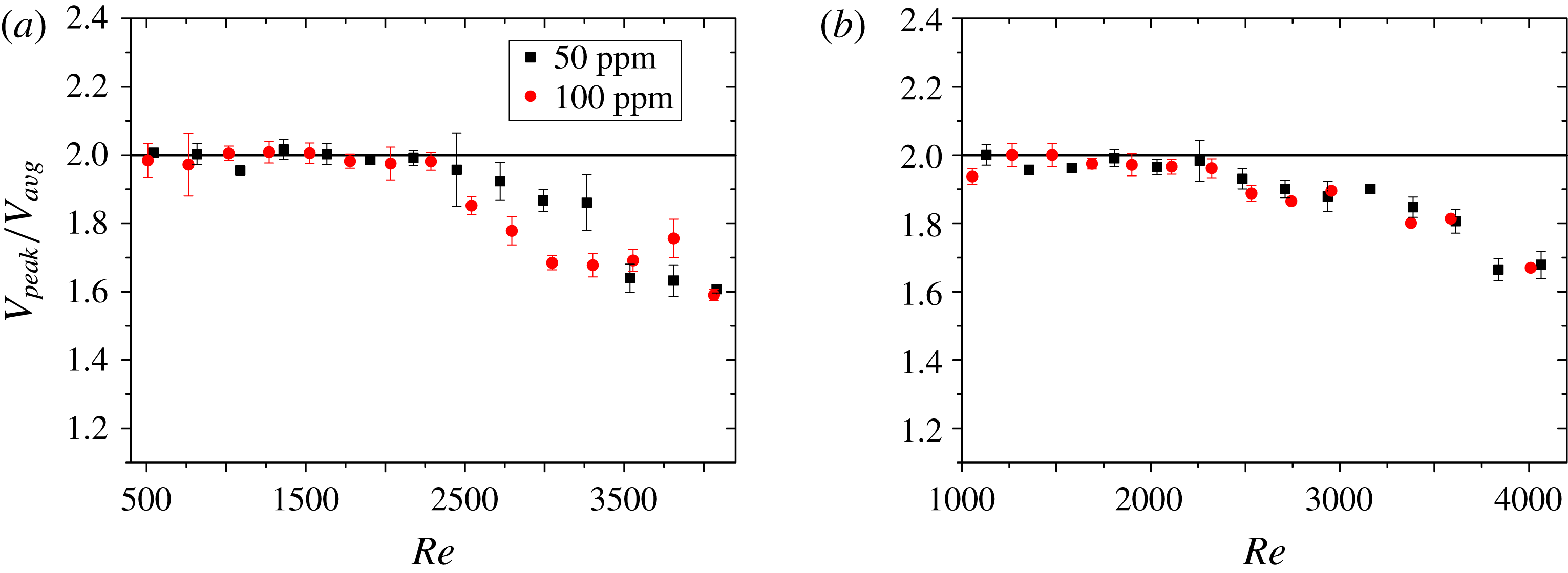
. At low polymer concentrations, as the concentration is increased in the range 50 ppm–100 ppm, it is observed that transition Reynolds number increases systematically from 2000 (for a Newtonian fluid) to approximately 2500 for the polymer solution. Furthermore, the nature of the variation of
 $V_{peak}/V_{avg}$
with
 $Re$
after transition is very different from that for a Newtonian fluid. There is no marked difference in the onset of the transition as we change the tube diameter (figure 9
b) except that the variation of
 $V_{peak}/V_{avg}$
with
 $Re$
seems to be gentler for
 $470~\unicode[STIX]{x03BC}\text{m}$
tubes. This could be attributed to the increased shear rates in tubes of smaller diameter at a given Reynolds number.
Comparison of time-averaged centre-line velocity for the flow of 50 ppm and 100 ppm polyacrylamide solution in tubes of diameters (a)
 $390~\unicode[STIX]{x03BC}\text{m}$
and (b)
 $470~\unicode[STIX]{x03BC}\text{m}$
. The horizontal line is the ratio of
 $V_{peak}/V_{avg}$
in the laminar regime.

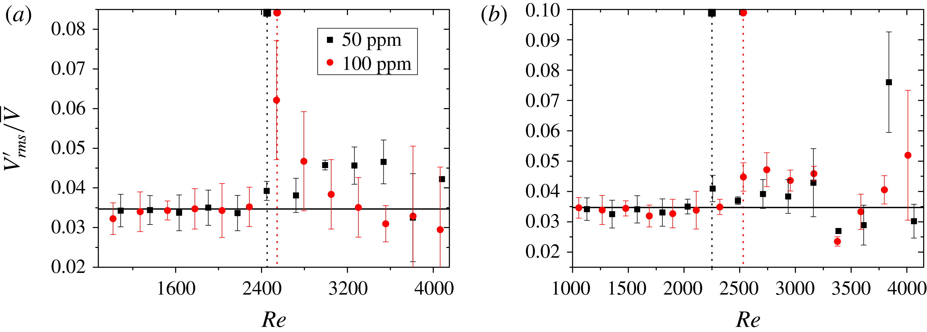
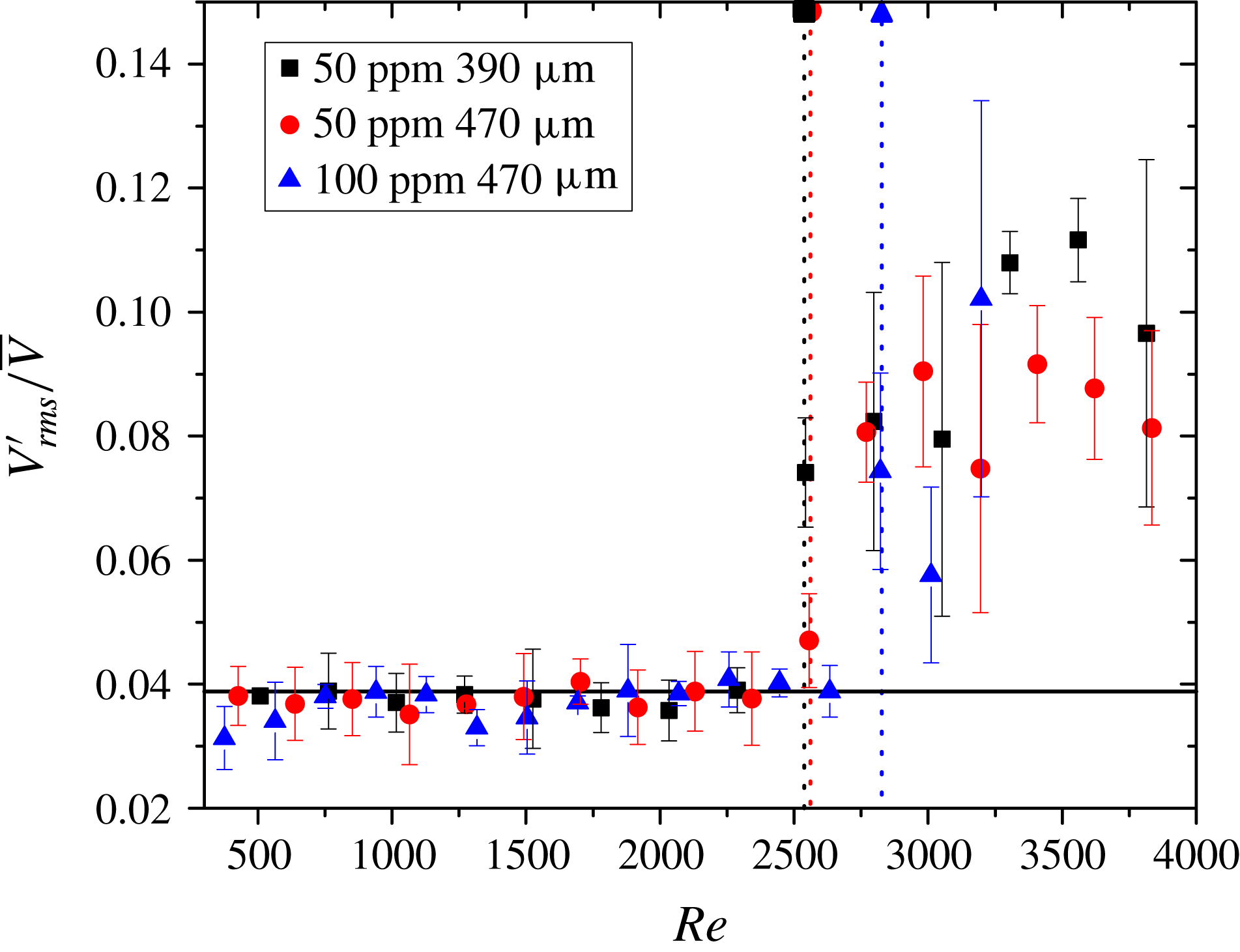
Comparison of magnitude of centre-line velocity fluctuations for 50 ppm and 100 ppm polyacrylamide solutions for flow in tubes of diameters (a)
 $390~\unicode[STIX]{x03BC}\text{m}$
and (b)
 $470~\unicode[STIX]{x03BC}\text{m}$
. The horizontal line is an indication of the magnitude of velocity fluctuations in the laminar regime. The vertical dotted line is an indicator of the transition
 $Re$
.

The earlier study of Srinivas & Kumaran (Reference Srinivas and Kumaran2017) observed that for channel flows, upon addition of small amounts of polymer, the velocity fluctuations are decreased even in the laminar regime. They also noted a decrease in velocity fluctuations in the post-transition regime. Figure 10 shows the normalized r.m.s. velocity fluctuations of the velocity (at the centre line) in the flow direction as a function of
 $Re$
. Beyond a certain
 $Re$
, there is a sharp increase in the magnitude of the r.m.s. velocity fluctuations, and this
 $Re$
is taken as the point of transition from laminar to turbulent flow. This Reynolds number value agrees reasonably with the Reynolds number at which there is a deviation of
 $V_{peak}/V_{avg}$
from its expected laminar value, thus corroborating the two different ways of marking the onset of transition. There is also a prominent decrease in the magnitude of the velocity fluctuations (compared to the Newtonian case) in the post-transition regime for low-concentration polymer solutions. There is no distinct change in the post-transition flow behaviour, with regard to velocity fluctuations, when we change the diameter of the tube from
 $390~\unicode[STIX]{x03BC}\text{m}$
to
 $470~\unicode[STIX]{x03BC}\text{m}$
(figure 10
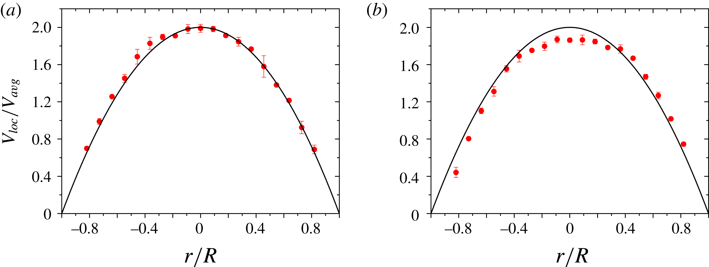
b). The velocity profile for a 100 ppm solution also becomes flatter in the post-transition regime (figure 11), but the profile is not as flat as in the case of a Newtonian fluid flow under a similar
 $Re$
range. The velocity profiles in the transition regime reveal a very small but consistent asymmetry in the radial direction, and similar observations were made for more concentrated solutions in the literature (Escudier et al.
Reference Escudier, Poole, Presti, Dales, Nouar, Desaubry, Graham and Pullum2005; Wen et al.
Reference Wen, Poole, Willis and Dennis2017).
Velocity profile comparison for (a) laminar (
 $Re=1500$
) and (b) transition regime (
 $Re=3000$
) of a 100 ppm polyacrylamide solution through a rigid microtube of diameter
 $470~\unicode[STIX]{x03BC}\text{m}$
. Here,
 $r$
is the coordinate in the direction perpendicular to the flow and
 $r=0$
denotes the tube centre. The continuous line represents theoretical velocity profile for a Newtonian fluid in the laminar regime and symbols represent the experimentally obtained velocity profile.

The variation of the velocity profile for a 100 ppm polyacrylamide solution through a
 $390~\unicode[STIX]{x03BC}\text{m}$
tube with increasing
 $Re$
. It is seen that the profile matches with the Newtonian velocity profile upto a certain
 $Re$
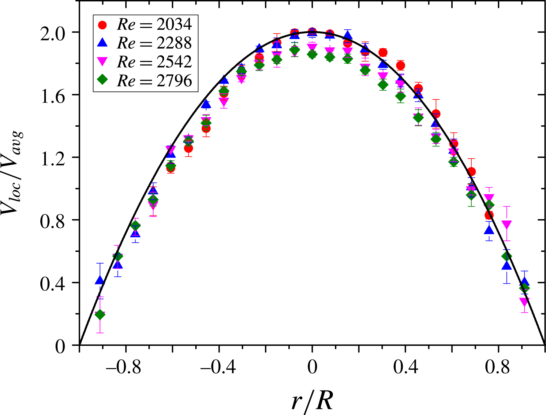
and then starts to become more flat. The continuous line represents theoretical velocity profile for a Newtonian fluid in the laminar regime and symbols represent the experimentally obtained velocity profile.

Figure 12 shows the evolution of velocity profiles with increasing
 $Re$
for the 100 ppm polyacrylamide solution. It is observed that the velocity profile matches with the theoretical velocity profile reasonably well up to
 $Re=2288$
. The velocity profile becomes flatter as we go to
 $Re=2542$
and higher. Theoretically, the area under these normalized velocity profiles should be
 $1/2$
. However, we find that the areas under the curves for different Reynolds number are slightly different from
 $1/2$
. This is a consequence of the use of
 $V_{avg}$
from volumetric flow-rate measurement in this study. If we had calculated
 $V_{avg}$
from the PIV data then the area under the normalized velocity profile would be very close to
 $1/2$
and the small errors encountered are due to fitting the data points. Thus, the discrepancy in the area in these curves is due to the difference in flow rates obtained from the PIV measurements and from direct volumetric flow-rate measurements. In the PIV measurements, it becomes increasingly difficult to measure velocity near the walls at high
 $Re$
. However, the difference in the area under the curve between the lowest
 $Re$
used and the highest transition
 $Re$
used is less than
 $3\,\%$
.
As the concentration of the added polymer is increased to 300 ppm (figure 13), the transition
 $Re$
decreases again, and is close to the Newtonian value of
 $2000$
. Beyond this critical concentration of polymer, the transition is initiated at a lower
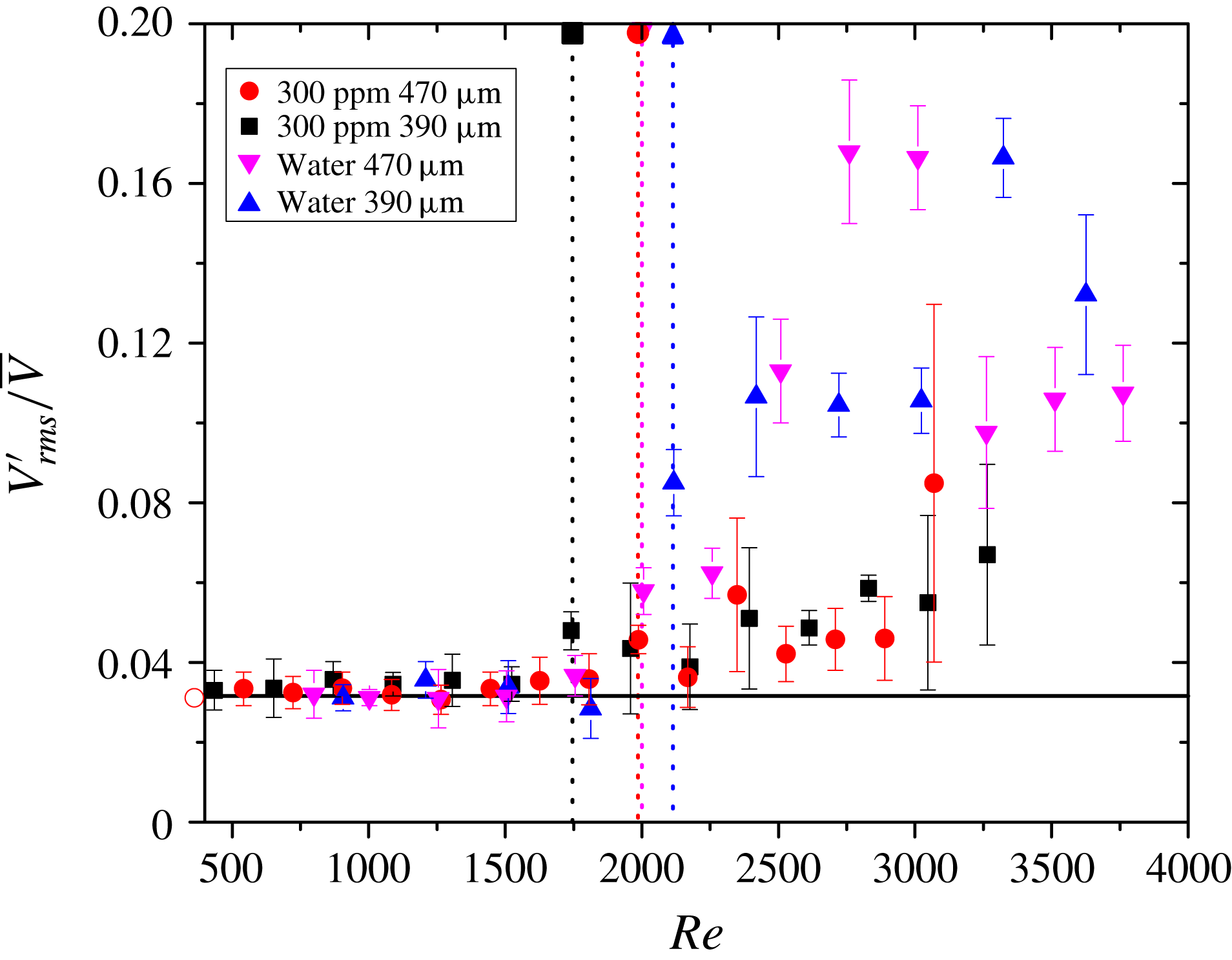
 $Re$
as compared to the Newtonian case. However, the post-transition characteristics are completely different for polymeric solutions and Newtonian fluids. For example, the velocity fluctuations are much lower for a polymeric solution (figure 13) as compared to Newtonian fluids. For the same concentration of polymer (i.e. 300 ppm), the transition happens at a lower
 $Re$
(figure 13) for the tube of diameter
 $390~\unicode[STIX]{x03BC}\text{m}$
compared to
 $470~\unicode[STIX]{x03BC}\text{m}$
, presumably because the elasticity numbers in the two cases are different due to the different diameters of the two tubes. This is markedly different from the Newtonian transition (figure 7), where the transition
 $Re$
is independent of tube diameter. The elasticity number is higher for the
 $390~\unicode[STIX]{x03BC}\text{m}$
tube, and transition occurs at a lower
 $Re$
for this tube compared to the
 $470~\unicode[STIX]{x03BC}\text{m}$
tube, suggesting that the transition characteristics are very different for a polymeric solution as compared to a Newtonian fluid.
Comparison of magnitude of centre-line velocity fluctuations in the flow of 300 ppm polyacrylamide solution with that in deionized water. The horizontal line is an indication of the magnitude of velocity fluctuations in the laminar regime. The vertical dotted line is an indicator of the transition
 $Re$
.

Comparison of time-averaged centre-line velocity of polyacrylamide solution (of concentrations 800 ppm, 600 ppm, 500 ppm) for flow in tubes of diameter (a)
 $390~\unicode[STIX]{x03BC}\text{m}$
and (b)
 $470~\unicode[STIX]{x03BC}\text{m}$
. The horizontal line is an indication of the ratio of
 $V_{peak}/V_{avg}$
in the laminar regime.

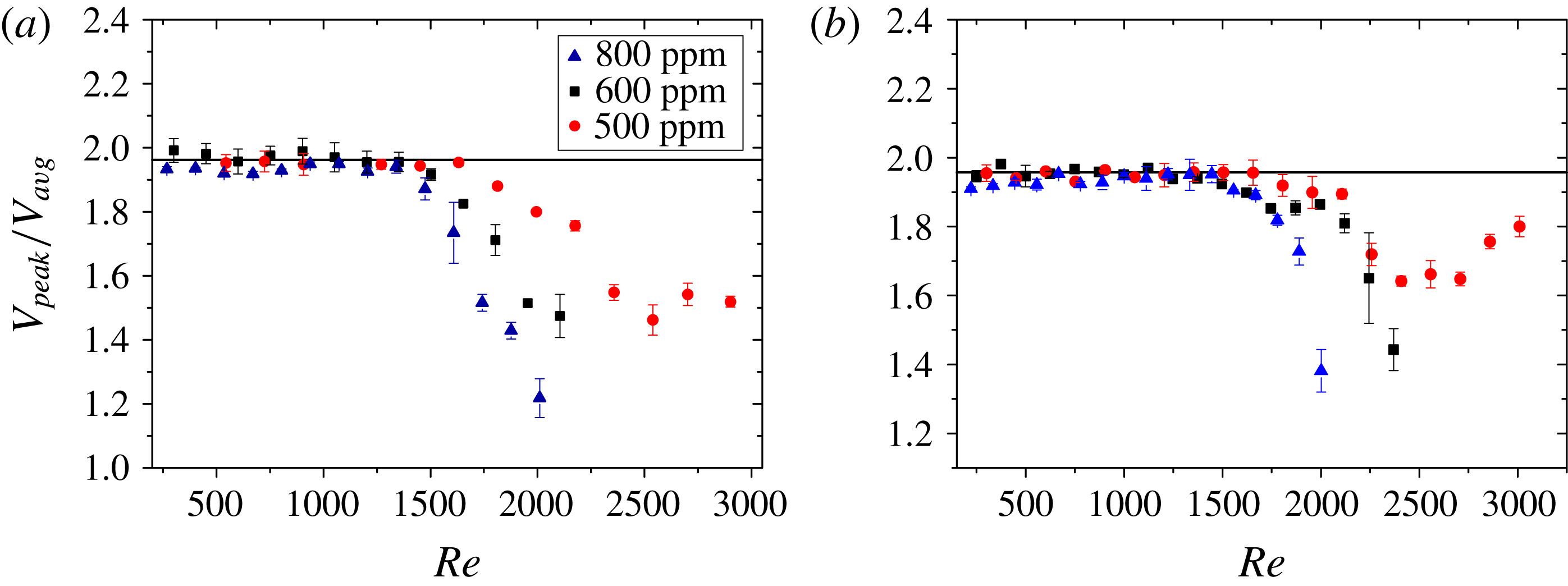
The time-averaged centre-line velocity for the flow of relatively higher concentration (in the range 500 ppm–800 ppm) polyacrylamide solution (figure 14
a) shows that, for such higher concentrations of the added polymer, the transition occurs at a lower
 $Re$
compared to pure deionized water. It is further observed that there is a shift of the non-dimensional parameter
 $V_{peak}/V_{avg}$
from its expected laminar value of 2 to approximately 1.95, which can be attributed to shear-thinning behaviour of the polymeric solution at the high shear rates (the nominal shear rate at
 $Re=500$
is approximately
 $5\times 10^{4}~\text{s}^{-1}$
) prevailing in the microtubes. Pinho & Whitelaw (Reference Pinho and Whitelaw1990) carried out experiments of highly shear-thinning sodium carboxymethyl cellulose solutions (with water as solvent), and they too observed that the ratio of centre-line to average velocity was lower than 2 for polymer solutions under laminar flow conditions. Changing the diameter of the tube enables us to operate at different shear rates in a comparable Reynolds number range. There appears to be a change in the variation of the ratio
 $V_{peak}/V_{avg}$
in the post-transition regime when we change the diameter of the tube (figure 14
b).
Comparison of centre-line velocity fluctuations in polyacrylamide solutions (800 ppm, 600 ppm, 500 ppm) for tubes of diameter (a)
 $390~\unicode[STIX]{x03BC}\text{m}$
and (b)
 $470~\unicode[STIX]{x03BC}\text{m}$
. The horizontal line is an indication of the laminar velocity fluctuation values. The vertical dotted line is an indicator of the transition
 $Re$
.

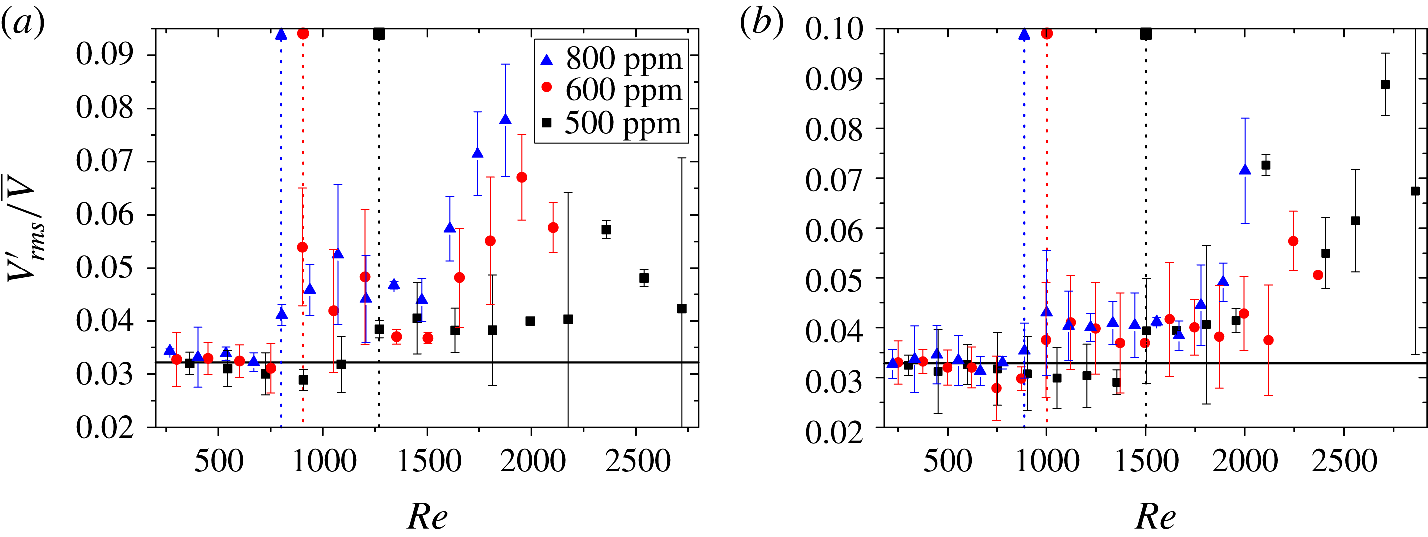
The magnitude of the centre-line velocity fluctuations (figure 15
a) reaffirms the trend that the transition
 $Re$
decreases from the Newtonian value of 2000 in agreement with the results from the time-averaged velocity profile. However, we are able to see variation in the
 $Re$
value for the onset of transition with the tube diameter, for the same polymer solution (figure 15
b). This can be ascribed to the increased shear rate in the smaller tube, leading to an increase in the elasticity number. Further, the magnitude of the velocity fluctuations in the transition regime is lower as compared to a Newtonian fluid.
Velocity profile comparison for laminar and transition regime in the flow of a 500 ppm polyacrylamide solution through a rigid microtube of diameter
 $470~\unicode[STIX]{x03BC}\text{m}$
: (a) flow at
 $Re=600$
and (b) at
 $Re=2400$
. Here,
 $r$
is the coordinate in the direction perpendicular to the flow and
 $r=0$
denotes the tube centre. The velocity profile is flatter after transition in flow of the polymeric solution. The continuous line represents the theoretical velocity profile for a Newtonian fluid in the laminar regime and symbols represent the experimentally obtained velocity profile.

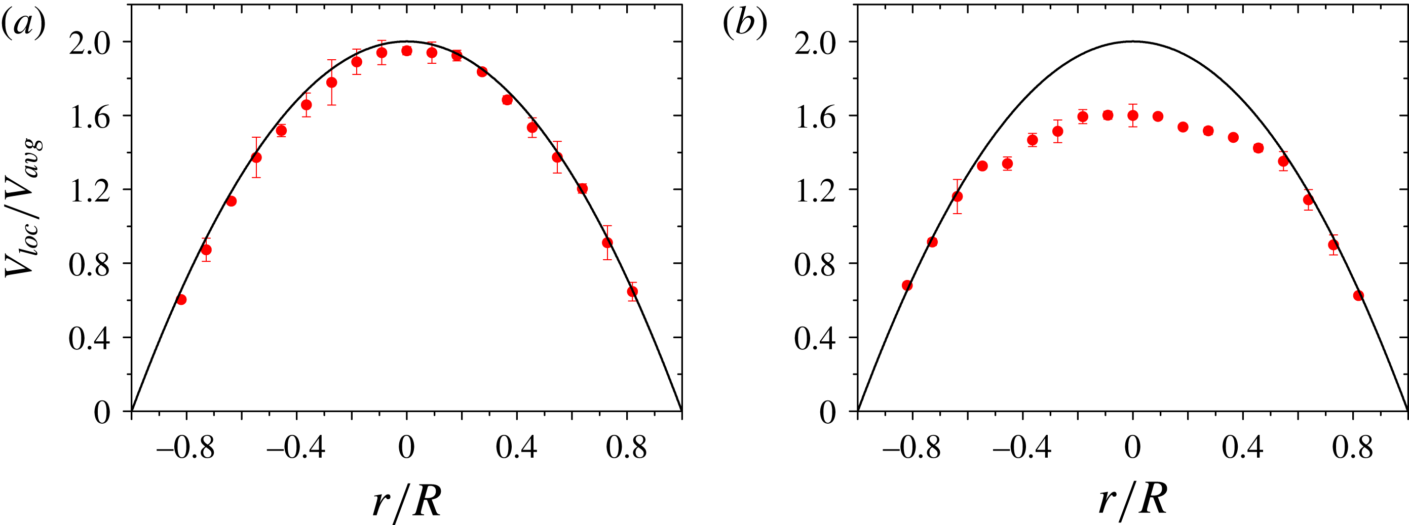
In the case of concentrated polymer solution (500 ppm) there is a modification in the velocity profile and it starts to become flatter near the centre line with increasing
 $Re$
(figure 16), compared to the case of the 100 ppm polymer concentration (figure 11), suggesting that the 500 ppm case is more turbulent at
 $Re=2400$
compared to the 100 ppm case at
 $Re=3000$
. In order to establish that the observed instability in the flow of polymer solutions is not because of the lower shear modulus of PDMS (compared to rigid materials like steel or glass) used to fabricate the tubes, we carried out experiments in tubes fabricated with PDMS of two different shear moduli. It is important to ascertain this, because it is known that when the shear moduli of the tubes are in the range of
 ${\sim}10~\text{kPa}$
, the deformable nature of the tube wall itself can induce new instabilities (Verma & Kumaran Reference Verma and Kumaran2012). We compared
 $V_{peak}/V_{avg}$
and the centre-line velocity fluctuations in tubes fabricated in
 $10\,\%$
PDMS tube (shear modulus
 ${\sim}0.35~\text{MPa}$
) and
 $15\,\%$
PDMS tube (shear modulus
 ${\sim}0.5~\text{MPa}$
). The data (not shown, in the interests of brevity) for the onset of transition for these two different tubes agreed reasonably well. Hence, we conclude that the shear modulus of the tube prepared plays no role in the onset of transition observed in our experiments.
3.2 Onset of transition in the flow of polyethylene oxide solutions
To establish the robustness of the observation that transition happens at
 $Re$
much lower than 2000 due to the added polymer, in this section, we discuss the results obtained using a different polymer, viz., polyethylene oxide with a
 $\text{molecular weight}=8\times 10^{6}$
. At low concentration of the added polymer, addition of the polymer delays transition in PEO solutions similar to the case of polyacrylamide solutions. However, the post-transition flow seems to be rather similar to the Newtonian fluid flow. There is no marked reduction in the magnitude of the fluctuations with PEO solution as seen from velocity fluctuations plot (figure 17). For higher concentrations, PEO solutions also exhibit an early transition at
 $Re<2000$
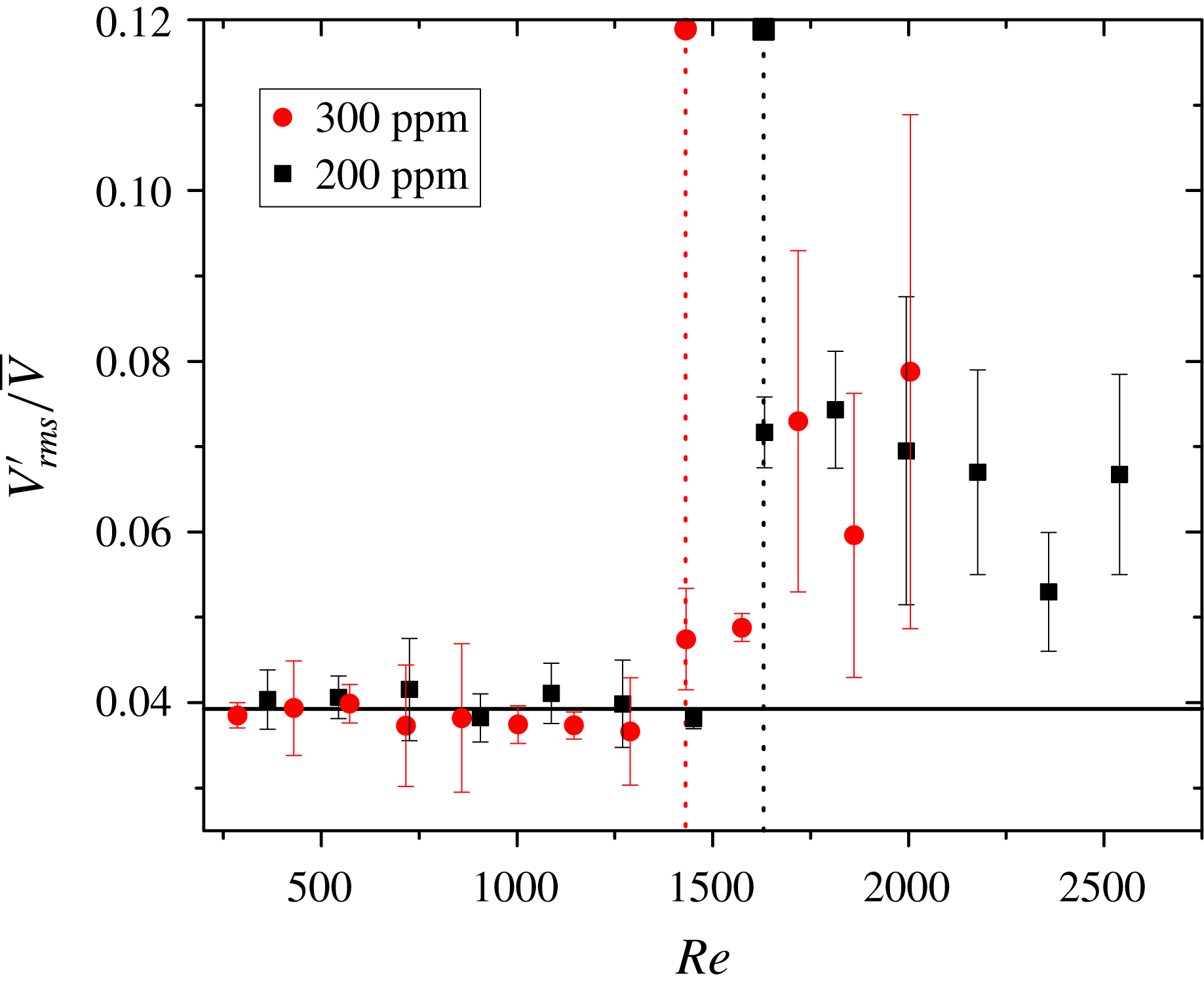
, similar to PAA solutions (figure 18). Hence PEO solutions exhibit a different post-transition flow behaviour (as compared to polyacrylamide), but the onset of transition is strikingly similar to polyacrylamide for solutions of similar viscosities. There is a shift in the value of
 $V_{peak}/V_{avg}$
from
 $2$
to approximately 1.95 in the average velocity data. This may perhaps be attributed to shear-thinning behaviour at high shear rates.
Comparison of centre-line velocity fluctuations in 50 ppm and 100 ppm polyethylene oxide solutions. The horizontal line is an indication of magnitude of velocity fluctuations in the laminar regime. The vertical dotted line is an indicator of the transition
 $Re$
.

Comparison of the velocity fluctuations at the centre line in high-concentration (300 ppm and 200 ppm) polyethylene oxide solutions. The horizontal line is an indication of the magnitude of velocity fluctuations in the laminar regime. The vertical dotted line is an indicator of the transition
 $Re$
.

Velocity profile comparison for laminar and transition regime of a 300 ppm PEO polymeric solution through a
 $390~\unicode[STIX]{x03BC}\text{m}$
rigid microtube: (a) flow at
 $Re=300$
and (b)
 $Re=1720$
. Here,
 $r$
is the coordinate in the direction perpendicular to the flow and
 $r=0$
denotes the tube centre. The velocity profile is flatter for post-transition flow of the polyethylene oxide solution. The continuous line represents the theoretical velocity profile for a Newtonian fluid in the laminar regime and symbols represent the experimentally obtained velocity profile.

Figure 19 shows that the velocity profile for PEO solution deviates from the Newtonian flow profile even at low
 $Re$
. This can attributed to the shear-thinning behaviour at such high shear rates at which the experiments are being performed. Studies performed on PEO solutions with viscosities close to polyacrylamide solutions show similar transition characteristics. Velocity fluctuations in the flow of PEO solutions also show early transition as compared to deionized water. These observations show that the phenomenon of early transition is quite robust, as the observations are similar for two different polymer solutions.
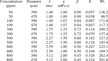
A comparison of different dimensional and non-dimensional parameters used for characterizing polyacrylamide solutions in the experiments. Here,
 $Wi_{t}$
is the Weissenberg number required for onset of transition in our experiments.

Reynolds number for transition for the two polymer solutions, i.e polyethylene oxide (MW
 $8\times 10^{6}$
), and polyacrylamide (MW
 $5\times 10^{6}$
), for different concentrations.

A comparison of different dimensional and non-dimensional parameters used for characterizing polyethylene oxide solutions in the experiments. Here,
 $Wi_{t}$
is the Weissenberg number required for onset of transition in our experiments.

3.3 Data collapse of experimental observations
It is instructive to examine whether the experimental observations obtained using two different polymer solutions and tubes of different diameters can be reduced into a single plot using suitable dimensionless groups.
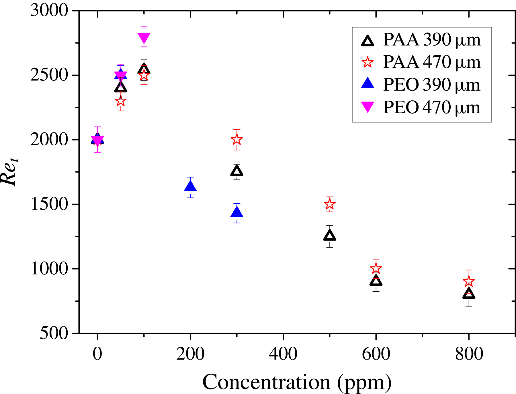
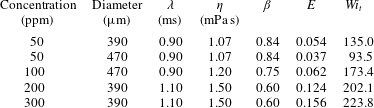
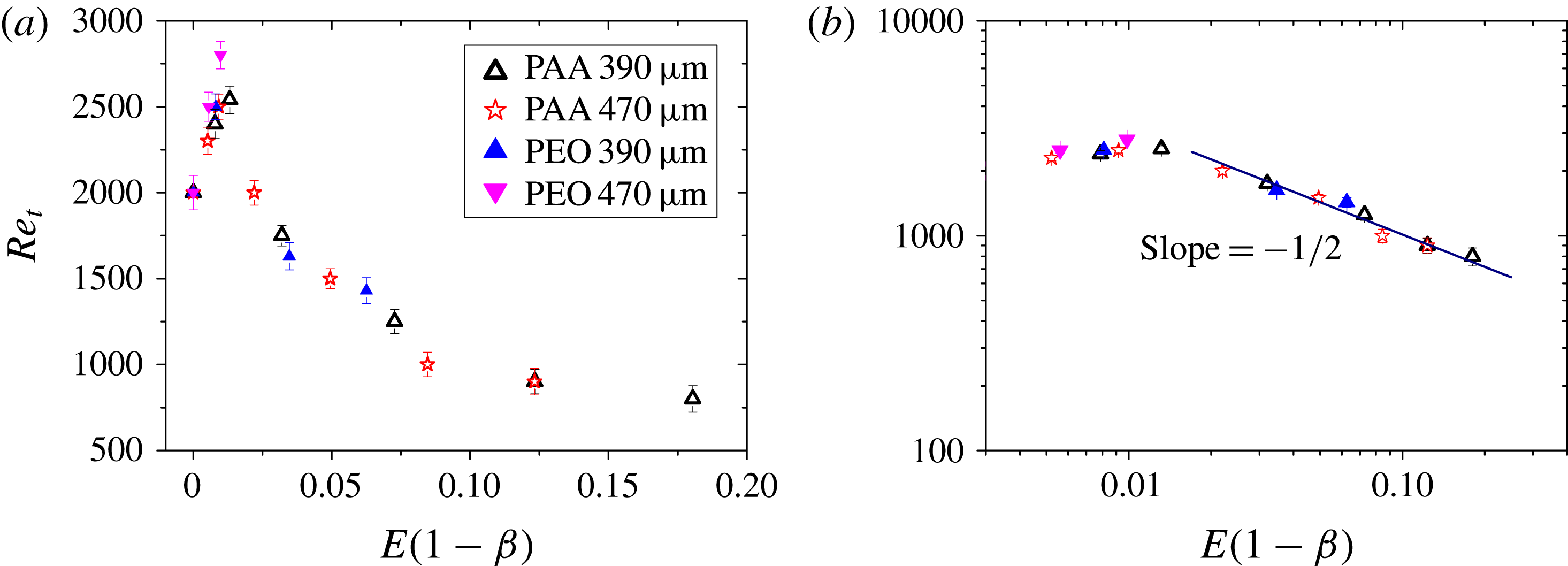
Tables 6 and 7 summarize the various dimensional and non-dimensional parameters for polyacrylamide and polyethylene oxide solutions used in our experiments. In addition, we also mention the Weissenberg number required for transition in our experiments. Figure 20 shows the variation of the transition Reynolds number with the concentration of the added polymer. There seems to be a critical concentration up to which the addition of polymer delays the transition, and beyond which addition of polymer tends to initiate transition at
 $Re$
lower than
 $2000$
, the transition
 $Re$
for a Newtonian fluid. From the standpoint of dimensional analysis, the transition
 $Re$
for the present system is a function of the elasticity number
 $E$
and the ratio of solvent to total viscosity
 $\unicode[STIX]{x1D6FD}$
. Here, it is assumed that the polymer solution is characterized only by its longest relaxation time. It is useful to plot the transition
 $Re$
in terms of the non-dimensional parameters
 $E$
and
 $\unicode[STIX]{x1D6FD}$
. The limits of
 $E\rightarrow 0$
and
 $\unicode[STIX]{x1D6FD}\rightarrow 1$
correspond to those of a Newtonian fluid. Instead of plotting
 $Re$
as a function of the two dimensionless variables
 $E$
and
 $(1-\unicode[STIX]{x1D6FD})$
separately, we propose to combine the two as
 $E(1-\unicode[STIX]{x1D6FD})$
, and
 $Re_{t}$
is plotted as a function of this product in figure 21(a). This combination can also be understood by the following physical argument (Poole Reference Poole2012). The usual Weissenberg number can be thought of as a ratio of elastic to viscous forces in a viscoelastic fluid. The elastic forces are proportional to the polymer viscosity while the viscous forces are proportional to the total viscosity. Thus, for polymer solutions, the relevant parameter is
 $(1-\unicode[STIX]{x1D6FD})\unicode[STIX]{x1D706}V/R$
. Thus, the dual limit of both
 $E\ll 1$
and
 $\unicode[STIX]{x1D6FD}\rightarrow 1$
represents the approach to a Newtonian fluid, and deviations from the Newtonian limit can be represented by the product
 $E(1-\unicode[STIX]{x1D6FD})$
. Here, the (longest) relaxation time of both the polymer solutions at different concentrations are taken from our small-amplitude oscillatory experiments. Plotted in this way, the transition
 $Re$
shows a reasonable data collapse with
 $E(1-\unicode[STIX]{x1D6FD})$
for tubes with different diameters, as well as for two different polymers at different concentrations of added polymer. The limit
 $E(1-\unicode[STIX]{x1D6FD})=0$
is the case of a Newtonian fluid, where the transition happens at
 $Re\sim 2000$
. Upon increase of
 $E(1-\unicode[STIX]{x1D6FD})$
, there is an initial increase in transition
 $Re$
, and after a further increase in
 $E(1-\unicode[STIX]{x1D6FD})$
, there is a decrease of transition
 $Re$
to as low as
 $800$
for the highest values of
 $E(1-\unicode[STIX]{x1D6FD})$
probed in our experiments. This plot thus shows that the ‘early’ transition observed for the two different polymer solutions can indeed be collapsed on a single curve, when plotted in terms of the suitable dimensionless combination
 $E(1-\unicode[STIX]{x1D6FD})$
. Based on this plot, it can be concluded that, for very small values of
 $E(1-\unicode[STIX]{x1D6FD})$
, the addition of very small amounts of polymer interferes with the finite-amplitude (subcritical) instability of a Newtonian fluid, but has a stabilizing effect on that transition. For sufficiently large values of
 $E(1-\unicode[STIX]{x1D6FD})$
, the role of added polymer is destabilizing in the regime of ‘early transition’ or elasto-inertial turbulence. When plotted in a
 $\log$
–
 $\log$
plot (figure 21
b), the data for
 $Re_{t}$
seem to scale as
 $1/\sqrt{E(1-\unicode[STIX]{x1D6FD})}$
in the regime where the polymer is destabilizing. It remains an open question whether this transition is due to an instability of the flow to infinitesimal disturbances, unlike in the case of a Newtonian fluid, where infinitesimal disturbances are always stable in the linear stability analysis. However, since the transition Reynolds number decreases with
 $E(1-\unicode[STIX]{x1D6FD})$
, it can be unambiguously inferred that fluid elasticity has a destabilizing effect on the transition.
Comparison of transition Reynolds number (
 $Re_{t}$
) with
 $E(1-\unicode[STIX]{x1D6FD})$
in a (a) linear plot and (b) log–log plot. Here
 $\unicode[STIX]{x1D6FD}$
is the ratio of solvent viscosity to the solution viscosity.

3.4 Dye-stream visualization
When injected in a laminar flow a dye stream remains straight but breaks up as soon as transition sets in the flow. The phenomenon is well documented for Newtonian flows (Verma & Kumaran Reference Verma and Kumaran2012; Neelamegam & Shankar Reference Neelamegam and Shankar2015) but surprisingly is not frequently used to visualize transition in the flow of polymer solutions. We first carried out dye-stream experiments for deionized water through a
 $470~\unicode[STIX]{x03BC}\text{m}$
microtube. A hollow (GI) tube is bent and placed at the centre of the tube just before the tube inlet. A needle of inner diameter
 ${\sim}100~\unicode[STIX]{x03BC}\text{m}$
is joined at the outlet of the GI tube using an adhesive (Araldite). The dye-stream experiments are performed by injecting a black-coloured water-soluble (Parker) dye stream of approximately
 $100~\unicode[STIX]{x03BC}\text{m}$
in diameter at the centre of the
 $470~\unicode[STIX]{x03BC}\text{m}$
microtube inlet. The dye is injected using a separate syringe pump (Fusion 200, Chemyx, Inc) and the flow rate of the dye stream is adjusted according to the
 $Re$
of the flow. Images are acquired at 1000 frames per second using Redlake MotionPro software by connecting a high-speed camera (Integrated Design Tools, SN:13-0907-0353, 1 megapixel) to a microscope (CKX41, Olympus, Japan). A 4
 $\times$
objective (PlanCN 4X) is used to magnify the view of the
 $470~\unicode[STIX]{x03BC}\text{m}$
microtube. A halogen bulb of high intensity is used to illuminate the
 $470~\unicode[STIX]{x03BC}\text{m}$
PDMS microtube. The phenomenon was first validated for a Newtonian fluid and then we performed a similar analysis for the flow of polymer solutions. We observe (figure 22) a breakup of the dye stream for a Newtonian fluid when we increase the
 $Re$
above 2000, which is in close agreement with our micro-PIV results for the Newtonian fluid. We carried out a similar experiment for a 800 ppm polyacrylamide solution through
 $470~\unicode[STIX]{x03BC}\text{m}$
tube and observed a breakup of the dye stream at
 $Re\sim 1040$
(figure 22). The velocity fluctuations as measured from the micro-PIV analysis showed a jump for the 800 ppm polyacrylamide solution through a
 $470~\unicode[STIX]{x03BC}\text{m}$
microtube at
 $Re\sim 926$
. Hence the results from our dye-stream experiments are consistent with the observations of our micro-PIV experiments. Since polymer solutions are prone to ageing, we performed all the dye-stream visualization experiments within 48 h of the preparation of the polyacrylamide solution. We were not able to perform dye-stream visualization experiments for tubes of diameter less than
 $470~\unicode[STIX]{x03BC}\text{m}$
.
Figure 23 shows the images obtained for the flow of 100 ppm PEO solutions. As shown in figure 17, the onset of transition happens at
 $Re\sim 2750$
. In figure 23, the dye-stream image for
 $Re=2600$
shows that the flow is laminar, while the image for
 $Re=2800$
shows that the dye stream has broken down, indicating the onset of transition. Thus, the dye-stream experiments corroborate both early transition for higher-concentration polymer solutions and the transition delay in polymer solutions of relatively lower concentration.
Snapshots of visualization using dye-stream injection in a
 $470~\unicode[STIX]{x03BC}\text{m}$
tube. (a) Movement of the dye stream for water in the laminar regime for
 $Re\sim 1750$
. (b) Motion of dye in water at
 $Re\sim 2250$
. (c) Motion of dye in a 800 ppm polyacrylamide solution at
 $Re\sim 810$
. (d) Motion of dye in a 800 ppm polyacrylamide solution at
 $Re\sim 1040$
. These snapshots show that for polymer solutions the transition happens at
 $Re$
much lower than
 $2000$
.

Snapshots of visualization using dye-stream injection in a
 $470~\unicode[STIX]{x03BC}\text{m}$
tube. (a) The image for 100 ppm PEO solution at
 $Re\sim 2600$
and (b) the image for 100 ppm PEO solution at
 $Re\sim 2800$
. These snapshots demonstrate that laminar flow is maintained at
 $Re\sim 2600$
and the transition happens only for
 $Re>2600$
.

4 Discussion
In this section, we place the experimental observations of the present study in the context of previous experimental studies that focused on transition in the flow of polymer solutions, and we make a comparative analysis of the results of all these studies. For the two polymers used in our study, viz., polyacrylamide (MW
 $5\times 10^{6}$
) and polyethylene oxide (MW
 $8\times 10^{6}$
), it is observed that as we increase the concentration of the polymer (from the case of pure Newtonian solvent), the transition Reynolds number increases from
 $2000$
(for the Newtonian solvent) to higher values up to a certain range of polymer concentration. There is marked reduction in velocity fluctuations in the post-transition regime due to the added polymer. It is observed that beyond this concentration limit there is a decrease in transition Reynolds number, and at the highest concentrations of polyacrylamide added (800 ppm), the transition
 $Re$
is as low as
 $800$
in our study. The transition studied in the present experiments is a natural transition which happens without any external forcing.
Goldstein et al. (Reference Goldstein, Adrian and Kreid1969) performed LDV measurements to calculate the ratio of centre-line velocity to mean velocity and normalized bandwidth for PEO solutions. It was observed that the ratio of centre-line velocity to mean velocity for PEO solutions is consistently lower than that for the Newtonian fluid for
 $Re<2000$
. The normalized bandwidth data also shows a jump below
 $Re=2000$
. It is important, however, to note that Goldstein et al. (Reference Goldstein, Adrian and Kreid1969) use water viscosity in calculating
 $Re$
for flow of PEO solutions, suggesting that if the actual polymer solution viscosity is used in the definition of
 $Re$
then the transition should happen at lower
 $Re$
values than reported by them. In our experiments, we too observe a similar phenomenon wherein there is a shift of ratio of centre-line velocity to mean velocity much below the Newtonian transition
 $Re$
of 2000, and there are some qualitative similarities between the present results and the earlier results of Goldstein et al. (Reference Goldstein, Adrian and Kreid1969). Forame et al. (Reference Forame, Hansen and Little1972) suggested that early transition could be achieved in large-diameter tubes (
 ${\sim}5.5~\text{mm}$
) if the wall shear stress is increased. High wall shear stress was achieved by the use of water–glycerine mixture as solvent for preparing PEO solutions. The solution prepared had a high viscosity (
 ${\sim}0.1~\text{Poise}$
) and hence higher wall shear stress. Since we use small-diameter tubes in our experiments, we are able achieve higher wall shear stress values with the use of low-viscosity solvent. We observe early turbulence by using higher-concentration polymer solution which is in qualitative agreement with Forame et al. (Reference Forame, Hansen and Little1972).
Samanta et al. (Reference Samanta, Dubief, Holzner, Schäfer, Morozov, Wagner and Hof2013) carried out experiments in the tube geometry using polyacrylamide solutions with the same molecular weight as used in the present study. Srinivas & Kumaran (Reference Srinivas and Kumaran2017) also used the same polymer, but used the rectangular channel geometry. When the concentration of the added polymer is the same for the present study and Samanta et al. (Reference Samanta, Dubief, Holzner, Schäfer, Morozov, Wagner and Hof2013), then
 $\unicode[STIX]{x1D6FD}$
is the same for the two studies and only the elasticity number is different between the present study and the work of Samanta et al. (Reference Samanta, Dubief, Holzner, Schäfer, Morozov, Wagner and Hof2013). The tube diameters used in Samanta et al. (Reference Samanta, Dubief, Holzner, Schäfer, Morozov, Wagner and Hof2013) are one order of magnitude larger than the tubes used in the present study. Since the polymer used is the same, this implies that the experiments of Samanta et al. (Reference Samanta, Dubief, Holzner, Schäfer, Morozov, Wagner and Hof2013) would correspond to a lower elasticity number
 $E=\unicode[STIX]{x1D706}\unicode[STIX]{x1D708}/R^{2}$
(due to the higher tube radii in their experiments) compared to the present experiments. Samanta et al. (Reference Samanta, Dubief, Holzner, Schäfer, Morozov, Wagner and Hof2013) focused on two different kinds of transition: in one case, the transition is forced (e.g. by fluid injection perpendicular to the laminar flow near the inlet), and in the other case, the flow was unperturbed, and the transition is natural as in the present study. Two different methods were used to characterize the transition. In the first method, pressure fluctuations were monitored in the tube, which exhibited a marked change near the transition. A jump in the (normalized) pressure fluctuations was considered as an indicator of transition. They also reported the variation of friction factor with Reynolds number, and the deviation of the friction factor from its expected laminar value is taken as an indicator of transition.
In the present study, the natural transition for pure water is observed at
 $Re\sim 2000$
, but Samanta et al. (Reference Samanta, Dubief, Holzner, Schäfer, Morozov, Wagner and Hof2013) observed that the natural transition for pure water occurred at
 $Re=6000$
whereas natural transition for a 100 ppm polymer solution was observed at
 $Re=3500$
. The reason for the higher values of Reynolds number for natural transition in their experiments could be because of the larger tube diameters used in their experiments, which allowed better disturbance-free inlet conditions in their set-up. However, in the present study and in the work of Sharp & Adrian (Reference Sharp and Adrian2004), the tube diameters are less than
 $500~\unicode[STIX]{x03BC}\text{m}$
, and in both cases, the natural transition for a Newtonian fluid occurred at
 $Re\sim 2000$
, as controlling the inlet conditions is difficult in such small geometries. Thus, the results of Samanta et al. (Reference Samanta, Dubief, Holzner, Schäfer, Morozov, Wagner and Hof2013) show that, for the unperturbed transition, there is a monotonous decrease in transition Reynolds number even for low concentrations. The scenario, however, is different for perturbed flow conditions in their experiments, where they observed that there is a critical concentration up to which transition is delayed and beyond which a new instability (termed ‘elasto-inertial’ turbulence) sets in. Further, Samanta et al. (Reference Samanta, Dubief, Holzner, Schäfer, Morozov, Wagner and Hof2013) noted that the
 $Re$
for the onset of elasto-inertial turbulence is independent of whether the transition is forced or natural. It was also shown that the onset of elasto-inertial turbulence scales with the shear rate and is independent of
 $Re$
. It must be noted that, for the case of pure water and 100 ppm polyacrylamide solution, the onset of a jump in pressure fluctuations coincided with the deviation of the friction factor from the laminar value. However, for the 500 ppm polyacrylamide solution, it was observed from the pressure fluctuation plot that the transition starts at
 $Re=800$
for a 4 mm diameter tube. The corresponding friction factor data of Samanta et al. (Reference Samanta, Dubief, Holzner, Schäfer, Morozov, Wagner and Hof2013) did not show any substantial deviation from the laminar value for
 $Re\sim 800$
, and the friction factor begins to deviate from the laminar result only beyond
 $Re=2000$
.
In contrast, our experiments do not contain any forcing mechanism for the instability, and hence we analyse only the natural transition of the flow. However, even in the case of a natural transition, for small amounts of the added polymer we observe a delay in the transition. Only after a significant increase in polymer concentration do we find a decrease in transition
 $Re$
. Furthermore, it is observed from the velocity fluctuations (at higher concentrations, i.e. 300 ppm and above) that transition occurs at lower
 $Re({<}2000)$
for higher shear rates. When specifically compared with the results of Samanta et al. (Reference Samanta, Dubief, Holzner, Schäfer, Morozov, Wagner and Hof2013), we do not observe transition at
 $Re=800$
(as in their case) for the 500 ppm polyacrylamide solution, despite the relatively larger elasticity numbers prevailing in our flow conditions. The lowest transition
 $Re$
observed in our case is
 ${\sim}800$
at a higher concentration of 800 ppm for polyacrylamide solution (MW
 $5\times 10^{6}$
). Thus, while there are qualitative similarities between the present results and those of Samanta et al. (Reference Samanta, Dubief, Holzner, Schäfer, Morozov, Wagner and Hof2013), there still remain some important quantitative differences.
Srinivas & Kumaran (Reference Srinivas and Kumaran2017) performed experimental investigations for high-molecular-weight polyacrylamide (MW
 $5\times 10^{6}$
) solutions through channels for polymer concentrations up to 50 ppm. The transition was inferred by a jump in the normalized velocity fluctuations, similar to the protocol used in this work. It was noticed that velocity fluctuations were reduced even in the laminar regime. Furthermore, the transition
 $Re$
was seen to be lower as compared to a Newtonian fluid (transition
 $Re=311$
for 50 ppm polyacrylamide solution). However, their study focused on rectangular channels. We too observe a decrease in velocity fluctuations upon addition of polymer in the post-transition regime; however, the transition
 $Re$
is quantitatively different. The difference in transition
 $Re$
could be attributed to the different flow geometries used in Srinivas & Kumaran (Reference Srinivas and Kumaran2017) and in the present study. But there are similarities in the results, in that the effect of addition of polymer is similar to that seen in Srinivas & Kumaran (Reference Srinivas and Kumaran2017) in terms of a lowering of the transition
 $Re$
, and in the decrease in velocity fluctuations in the post-transition regimes.
5 Conclusions
Experiments have been carried out using the micro-PIV technique to characterize the onset of instability and transition in the flow of polymer solutions in microtubes of diameters
 $390~\unicode[STIX]{x03BC}\text{m}$
and
 $470~\unicode[STIX]{x03BC}\text{m}$
, with two different polymer solutions (of varying concentrations), viz., polyacrylamide and polyethylene oxide solutions in water. For small concentrations of the added polymer, there is a consistent delay in the transition compared to that of the pure Newtonian solvent. However, beyond a certain concentration, the transition occurs at a
 $Re$
value lower than 2000, and for the largest concentrations probed in this work (800 ppm polyacrylamide solutions), the transition
 $Re$
could be as low as
 ${\sim}800$
. The characterization of the transition in polymer solutions has been done using the deviation of the ratio of centre-line to average velocity from its laminar value, and by observing the magnitude of velocity fluctuations and locating the
 $Re$
at which they undergo a sudden increase. The onset of transition is also further verified using dye-stream visualization. The data for transition
 $Re$
obtained using tubes of different diameters, two different polymers, and for different concentrations of the added polymer, collapse well when plotted in terms of the dimensionless combination
 $E(1-\unicode[STIX]{x1D6FD})$
. Our experimental data for the transition
 $Re$
(denoted as
 $Re_{t}$
) seem to be well approximated by the scaling relation
 $Re_{t}\propto 1/\sqrt{E(1-\unicode[STIX]{x1D6FD})}$
in the regime where there is early transition. This shows that the transition observed is quite robust, and is independent of the nature of the polymer added. The present study thus provides further evidence for ‘early transition’ in the flow of polymer solutions, where transition occurs at
 $Re$
much lower than
 $2000$
, the transition Reynolds number for Newtonian fluids. The present observations, along with recent experimental studies of Samanta et al. (Reference Samanta, Dubief, Holzner, Schäfer, Morozov, Wagner and Hof2013) and Srinivas & Kumaran (Reference Srinivas and Kumaran2017), respectively, for flow in tubes and rectangular channels, suggest that the early transition at
 $Re$
much less than
 $2000$
could be a generic feature in polymeric solutions at sufficiently high values of elasticity number easily realized when the smallest length scale is of the order of a few hundred micrometres. This early transition occurs due to a destabilizing effect of elasticity of the polymer solution, and hence is qualitatively different from the transition in the flow of Newtonian fluids.
Acknowledgements
The authors thank the Department of Science and Technology, Government of India (grant EMR/2016/001218), for financial support. The authors acknowledge the SEM facility of the Department of Material Science and Engineering, Indian Institute of Technology, Kanpur. The authors thank Professor V. Kumaran, Professor G. Subramanian, Dr T. Bhuvana, Dr D. Sharma, Mr P. Rajvanshi, Mr S. Kumar Rout, Mr K. Bharadwaj, Mr R. Patne and Mr P. Joshi for providing insights and useful suggestions while conducting the experiments.