3.1 Trim state

As mentioned earlier, flight envelopes of the previously generated database, which is used in this research, are actually maneuvering flight envelopes, which mean they are boundaries containing steady state maneuvers. Such steady state maneuvers are referred to as trim points in this research.

A steady state maneuver is the condition in which all linear and angular velocity rates and aerodynamic angles rates are zero^{(Reference Stevens, Lewis and Johnson38)}. Hence, in the wind-axes coordinate system:

(1) \begin{equation}\left( {\dot V,\dot \alpha ,\dot \beta } \right) \equiv \left( {\dot p,\dot q,\dot r} \right) \equiv 0\end{equation}

where, V, $\alpha $ and $\beta $ are the aircraft total airspeed, angles of attack and sideslip, and $p,q,r$ , are the roll rate, pitch rate and yaw rate, respectively.

Since the considered steady state maneuvers are in fact level/climbing/descending rectilinear and turning flights, hence

(2) \begin{equation}\dot \phi ,\dot \theta = 0,{\rm{\;\;\;\;}}\gamma = {\gamma^{\ast}},\;\;\;\dot \psi = {\dot \psi^{\ast}}\end{equation}

where, $\phi ,\theta ,\psi ,$ and $\gamma $ are the roll (bank) angle, pitch angle, yaw (heading) angle, and the flight path angle. Also, ${\gamma^{\ast}},\;{\dot \psi^{\ast}}$ are the desired constant values defining the steady state maneuvers.

In terms of the nonlinear aircraft equations of motion:

(3) \begin{equation}{\dot x_{trim}} = f\left( {{x_{trim}},{\rm{\;}}{u_{trim}}} \right) = 0\end{equation}

(4) $${x_{trim}} = {\left[ {V,\alpha ,\beta ,p,q,r,\phi ,\theta } \right]^T} = \;{x^ * }$$

(5) $${u_{trim}} = {\left[ {{\delta _{th}},{\delta _e},{\delta _a},{\delta _r}} \right]^T} = \;{u^ * }$$

where $f$ is a vector of nonlinear functions, x is the state vector, u is the control vector, and ${\delta _{th}}$ , ${\delta _e}$ , ${\delta _a}$ , and ${\delta _r}$ represent engine throttle setting and deflections in the elevator, aileron, and rudder, respectively.

Maneuvering flight envelopes are composed of trim states characterised by four parameters 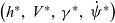$\left( {{h^{\ast}},\;{V^{\ast}},\;{\gamma^{\ast}},\;{{\dot \psi}^{\ast}}} \right)$ . These flight envelopes can be depicted as three-dimensional volumes at each constant flight altitude ${h^{\ast}}$ ^{(Reference Norouzi, Kosari and Sabour4)}. Hence, each trim point should be derived by solving all the aircraft nonlinear equations of motion ( ${\dot x_{trim}} = 0)$ for the intended flight path angle and turn rate $\left({{\gamma^{\ast}},\;{{\dot \psi}^{\ast}}} \right)$ at the considered airspeed ( ${V^{\ast}}$ ) and altitude ( ${h^{\ast}}$ ).

3.2 Computational procedure

Since this is not analytically possible, the corresponding constrained nonlinear optimisation problem is numerically solved, in which the cost function is^{(Reference Strube21,Reference Tang, Atkins and Sanner24,Reference Stevens, Lewis and Johnson38)} :

(6) \begin{equation}J\left({x,u} \right) = {\raise0.7ex\hbox{$1$} \!\mathord{\left/{\vphantom {1 2}}\right.}\!\lower0.7ex\hbox{$2$}}\dot x_{trim}^T\ Q{\dot x_{trim}}\end{equation}

where $Q$ is a positive definite weighting matrix which specifies the contributions of the state derivatives to the cost function. $J$ is subject to the following equality and inequality constraints:

(7) \begin{equation}h - {h^{\ast}} = 0\end{equation}

(8) \begin{equation}V - {V^{\ast}} = 0\end{equation}

(9) \begin{equation}tan\theta - \frac{{ab + sin{\gamma^{\ast}}\sqrt {{a^2} - si{n^2}{\gamma^{\ast}} + {b^2}} }}{{{a^2} - si{n^2}{\gamma^{\ast}}}} = 0,\quad \theta \ne \pm \pi /2\end{equation}

where

(10) \begin{equation}a = cos\alpha\ cos\beta ,{\rm{\;\;\;}}b = sin\phi\ sin\beta + cos\phi\ sin\alpha\ cos\beta \end{equation}

(11) \begin{equation}p + {\dot \psi^{\ast} sin\theta=0}\end{equation}

(12) \begin{equation}q - {\dot \psi^{\ast}}cos\theta\ sin\phi = 0\end{equation}

(13) \begin{equation}r - {\dot \psi^{\ast}}cos\theta\ cos\phi = 0\end{equation}

(14) \begin{align}\begin{array}{cc}{\left| {{\delta _{th}} - 0.5} \right| \le 0.5}&{\left| {{\delta _e}} \right| \le 30}\\{\left| {{\delta _a}} \right| \le 20}&{\left| {{\delta _r}} \right| \le 30}\end{array}\end{align}

To construct the database used in this research, the aforementioned constrained optimisation problem was iteratively solved via the sequential quadratic programming (SQP) technique with a convergence criterion of 10⁻⁷.

3.3 Linearisation and stability evaluation

At the final step, the stability of the derived feasible trim points are checked as being feasible is not adequate for a trim state to include it in the maneuvering flight envelope and being stable is the sufficient condition.

By definition, a nonlinear system is considered stable at a specific trim point if it inherently converges to that trim state when being in the vicinity of the trim point^{(Reference Khalil39)}.

To evaluate the stability of the aircraft at a derived trim point ${x^{\ast}}$ , the aircraft equations of motion are linearised about ${x^{\ast}}$ via a perturbation method. Generally, multivariate Taylor series expansion of the nonlinear state equations of the aircraft ( ${\dot x} = f\left( {{x},{\rm{\;}}{u_{\rm{\;}}}} \right)$ ) around a trim point ( ${x^{\ast}}$ , ${u^{\ast}}$ ) and retaining just the first-order terms gives

(15) \begin{equation} \dot x + \delta \dot x = \;f\left( {{x^{\ast}},{u^{\ast}}} \right) + {\raise0.7ex\hbox{${\partial f}$} \!\mathord{\left/{\vphantom {{\partial f} {\partial x}}}\right.}\!\lower0.7ex\hbox{${\partial x}$}}\delta x + {\raise0.7ex\hbox{${\partial f}$} \!\mathord{\left/{\vphantom {{\partial f} {\partial u}}}\right.}\!\lower0.7ex\hbox{${\partial u}$}}\delta u\end{equation}

where $\delta x = x - {x^{\ast}}$ , $\delta u = u - {u^{\ast}}$ are small perturbations from the trim condition. Also, according to the equation (3) ${\dot x_{trim}} = f\left( {{x^{\ast}},{u^{\ast}}} \right) = 0$ , hence

(16) \begin{equation}\delta \dot x = {\raise0.7ex\hbox{${\partial f}$} \!\mathord{\left/{\vphantom {{\partial f} {\partial x}}}\right.}\!\lower0.7ex\hbox{${\partial x}$}}\delta x + {\raise0.7ex\hbox{${\partial f}$} \!\mathord{\left/{\vphantom {{\partial f} {\partial u}}}\right.}\!\lower0.7ex\hbox{${\partial u}$}}\delta u\end{equation}

which is in the form of the linear state — space equation ( $\dot X = AX + BU$ ) in which uppercase symbols denote perturbations from the trim point. Therefore the partial derivative terms ( ${\raise0.7ex\hbox{${\partial f}$} \!\mathord{\left/{\vphantom {{\partial f} {\partial x}}}\right.}\!\lower0.7ex\hbox{${\partial x}$}}{\rm{\;}},{\raise0.7ex\hbox{${\partial f}$} \!\mathord{\left/{\vphantom {{\partial f} {\partial u}}}\right.}\!\lower0.7ex\hbox{${\partial u}$}}$ ) denote Jacobian matrices $A,B$ that express the linear sensitivities of $f$ to perturbations in $x,u$ and are evaluated at the considered trim point:

(17) \begin{equation}\begin{array}{c}A=\left. {\partial f}/ {\partial x} \right]_{x^{\ast},u^{\ast}}= \left.\left[ \begin{array}{c@{\quad}c@{\quad}c} {\partial f_1}/ {\partial x_1} & \cdots & {\partial f_1}/ {\partial x_n}\\[3pt] \vdots & \ddots & \vdots\\[3pt] {\partial f_n}/ {\partial x_1} & \cdots & {\partial f_n}/ {\partial x_n}\\\end{array}\right]^{\vphantom{\frac{1}{2}}}\!\!\right]_{x^{\ast},u^{\ast}} \\[12pt] B=\left. {\partial f}/ {\partial u} \right]_{x^{\ast},u^{\ast}}= \left.\left[ \begin{array}{c@{\quad}c@{\quad}c} {\partial f_1}/ {\partial u_1} & \cdots & {\partial f_1}/ {\partial u_m}\\[3pt] \vdots & \ddots & \vdots\\[3pt] {\partial f_n}/ {\partial u_1} & \cdots & {\partial f_n}/ {\partial u_m}\\\end{array}\right]^{\vphantom{\frac{1}{2}}}\!\!\right]_{x^{\ast},u^{\ast}}\end{array}\end{equation}

$n,m$ are dimensions of the state and control vectors, respectively.

There are two approaches to evaluate the first partial derivatives that make up the Jacobian matrices. The first approach is to compute the symbolic derivation of each element of the vector $f$ with respect to the corresponding element of the vector $x$ or $u$ . This will lead to dimensional aerodynamic derivatives within the Jacobian matrices which in turn should be calculated using the non-dimensional stability and control derivatives. This requires having each of the non-dimensional forces and moments coefficients in the form of an analytical multivariate function of different variables (such as aerodynamic angles, Mach number, and altitude), so that the mathematical expression for each of the non-dimensional stability and control derivatives could be derived analytically. However, in the case of high-fidelity models where aerodynamic and propulsion data are provided in tabular form (as in the case of the GTM used in this research), such differentiable analytical functions are not available and the aforementioned first derivatives must be evaluated numerically^{(Reference Stengel40)}.

Hence, as the second approach, the first partial derivatives are conventionally and more conveniently approximated by using finite differences ^{(Reference Stevens, Lewis and Johnson38)}. To be specific, forward finite differences have been used in this research to evaluate the elements of the Jacobian matrices:

(18) \begin{equation}\begin{array}{c} {\raise0.7ex\hbox{${\partial {f_i}}$} \!\mathord{\left/{\vphantom {{\partial {f_i}} {\partial {x_j}}}}\right.}\!\lower0.7ex\hbox{${\partial {x_j}}$}} \approx {\raise0.7ex\hbox{${\left( {{\,f_i}\left( {{x^{\ast}} + \varepsilon {e_j},{u^{\ast}}} \right) - {f_i}\left( {{x^{\ast}},{u^{\ast}}} \right)} \right)}$} \!\mathord{\left/{\vphantom {{\left( {{f_i}\left( {{x^{\ast}} + \varepsilon {e_j},{u^{\ast}}} \right) - {f_i}\left( {{x^{\ast}},{u^{\ast}}} \right)} \right)} \varepsilon }}\right.}\!\lower0.7ex\hbox{$\varepsilon $}}\\[12pt] {\raise0.7ex\hbox{${\partial {f_i}}$} \!\mathord{\left/{\vphantom {{\partial {f_i}} {\partial {x_{j^{x}}}}}}\right.}\!\lower0.7ex\hbox{${\partial {u_k}}$}} \approx {\raise0.7ex\hbox{${\big( {{\,f_i}\left( {{x^{\ast}},{u^{\ast}} + \varepsilon {e_k}} \right) - {f_i}\left( {{x^{\ast}},{u^{\ast}}} \right)} \big)}$} \!\mathord{\left/{\vphantom {{\left( {{f_i}\left( {{x^{\ast}},{u^{\ast}} + \varepsilon {e_k}} \right) - {f_i}\left( {{x^{\ast}},{u^{\ast}}} \right)} \right)} \varepsilon }}\right.}\!\lower0.7ex\hbox{$\varepsilon $}}\end{array}\end{equation}

in which, $\varepsilon $ is a positive and small number (10⁻⁶ in this research), and ${e_j},\;{e_k}$ are the ${j^{th}}$ and ${k^{th}}$ columns of identity matrices of the same sizes of the ${x^{\ast}},{u^{\ast}}$ , respectively.

System eigenvalues determine if the considered trim point is stable. While stability is more preferable as the aircraft naturally tends to damp the effect of small disturbances, an unstable trim point still can be included in the flight envelope if it is controllable, which is evaluated by the linearised system’s controllability matrix $C$ :

(19) \begin{equation}C = \left[ {B{\rm{\;\;\;\;}}AB{\rm{\;\;\;\;}}{A^2}B{\rm{\;\;\;\;}} \cdots {\rm{\;\;\;}}{A^{n - 1}}B} \right]\end{equation}

3.4 Additional considerations

3.4.1 Bank angle

According to the Section 1, one of the main reasons for the impaired aircraft’s maneuvering flight envelope estimation is the post-failure path planning.

The load factor ( $n$ ) increases with increasing airplane bank angle, making turns less comfortable for passengers:

(20) \begin{equation}n = 1/cos\phi \end{equation}

Hence, it is preferable for commercial transport aircraft to use bank angles not exceeding 30 degrees and very much less in the final approach and landing phases. This enables shallow turns which impose small $g$ -forces (up to 1.2 $g$ ) on passengers. For instance, in Ref. (Reference Tang, Atkins and Sanner24), an adaptive flight planner that selects trim points from the estimated flight envelopes was applied to a wing damaged GTM for the post-failure path planning in the landing phase, and a 30° bank constraint was imposed on the path planner to have shallow turns to the final approach. Also, in Ref. (Reference Asadi, Sabzehparvar and Talebi25), maneuvering flight envelopes were estimated for bank angles constrained to ±20°. Likewise in Ref. (Reference Lombaerts, Schuet, Acosta and Kaneshige41), a 35° bank constraint was imposed on the online flight envelope determination of an Airbus A300 full-scale model. Therefore, a 30° bank constraint was imposed on the trim points derivation of the utilised database. This way, the estimated MFEs are composed of trim points which all require bank angles equal to or less than 30°. It should be noted that such constraint does not mean that the aircraft is incapable of flying with banks more than 30°. However, it was imposed to derive trim points that are all capable of being implemented by the flight management system and the autopilot, and also to investigate how far the aircraft can maneuver satisfying this constraint. Perhaps, other researchers can estimate the GTM flight envelopes with bank angles up to 60° structural limit or up to any other degree based on their research goal.

5.1 Unimpaired flight envelopes

Figures 1–4 show 3D maneuvering flight envelopes estimated for the unimpaired GTM in various flight path angles and flying altitudes. These are 4 out of the 168 3D MFEs estimated for the GTM. The rest 164 3D MFEs, which belong to the considered impaired cases, are presented in Ref. (Reference Norouzi, Kosari and Sabour43).

Figure 1.

Unimpaired case at sea level.

Figure 2.

Unimpaired case at 10,000ft.

Figure 3.

Unimpaired case at 20,000ft.

Figure 4.

Unimpaired case at 30,000ft.

Figure 5 depicts the 2D maneuvering flight envelope of the unimpaired GTM at sea level and zero flight path angle. Each blue dot represents a feasible — stable or feasible — controllable trim point. It also shows different sections of the unimpaired flight envelope boundary highlighted by their limiting factors. Limiting factor means a determinative parameter which hampers the access to further trim points. Such limiting factors are either a state or a control. Identifying these limiting factors and understanding their variation trends; help in better comprehension and prediction of the changes in flight envelopes due to failures.

Figure 5.

Flight envelope boundary sections for unimpaired case at sea level and zero flight path angle.

Hence, in this section, the results of a rigorous analysis made on the unimpaired flight envelope boundary of the GTM are presented.

In Fig. 5, the magenta-coloured section is the stall boundary, in which no further trim point is admissible, because further trim points would have angles of attack higher than the 10.5° critical angle-of-attack. Therefore in this section, the limiting factor is the angle-of-attack. The green-coloured section represents the aileron saturation boundary, where further trim points would require aileron deflections greater than +20° or −20°. This section’s limiting factor is the aileron’s deflection angle. The red-coloured section shows thrust saturation boundary, which is composed of trim points with maximum throttle setting. Further trim points would require amounts of thrust bigger than the engines’ available thrust.

To accurately understand what is going on in these boundaries and why they have these limiting factors, the states and controls variations along the trim points of these boundaries were investigated.

To do so, the analysis started from the rectilinear non-sideslipping maneuver of the lowest speed in the flight envelope, continued on the left half of the flight envelope boundary, up to the rectilinear non-sideslipping maneuver of the highest speed in the flight envelope (i.e. from $V = 58,\;\dot \psi = 0$ to $V = 176,\;\dot \psi = 0$ ). Due to symmetry of the flight envelope, results of this investigation are valid for the other half of the boundary.

Figures 6–11 show variations of $\alpha ,\;\;T$ (which is the required thrust), $\phi ,\;\;\beta ,\;\;{\delta _a},\;\;{\delta _r},$ along the trim points of the flight envelope boundary. In each figure, the variation of a state or a control with the flight envelope boundary speed is plotted. Since speed is increasing almost linearly along trim points in most parts of the boundary, speed is chosen as the horizontal axis of these plots, rather than turn rate. An exception to this is the stall boundary section, in which, the primary changing variable is turn rate, whereas speed is constant with respect to different values of turn rate in many sections of the stall boundary. This exception has resulted in congestions in the stall boundary section of most of the presented plots. To enhance the visualisation of these plots, zoomed-in-plots of the congested areas are provided inside each figure. Since these zoomed-in-plots are mainly composed of $V$ -constant sections, to have a better insight, the corresponding variations in turn rate are also plotted next to the in-plots (in blue), for the same trim points.

Figure 6.

Variation of angle-of-attack with boundary trim points.

Figure 7.

Variation of bank angle with boundary trim points.

Figure 8.

Variation of angle of sideslip with boundary trim points.

Figure 9.

Variation of aileron deflection angle with boundary trim points.

Figure 10.

Variation of rudder deflection angle with boundary trim points.

Figure 11.

Variation of thrust-required with boundary trim points.

By moving from the starting point of the boundary analysis (at the bottom of the envelope) to the end point (at the top of the envelope), and investigating Figs. 6–11 attentively, the airplane’s behaviour can be described as below:

The airplane initiates coordinated (zero sideslip) left turn (negative turn rates) via banking to the left (negative roll angle). To increase turn rates, it banks more to the left until the bank angle is saturated (30° bank constraint). From this point onwards, to access higher turn rates, the airplane enters slipping (non-coordinated) turn in which it yaws to the left (increases sideslip) via increasing positive rudder input. However, this would result in an adverse negative roll, which increases bank angle if not compensated. Therefore, the airplane counteracts the adverse roll and maintains a 30° degree bank angle through increasing negative aileron input. The airplane achieves higher turn rates in this manner until the aileron becomes saturated (end of the stall boundary, beginning of the aileron saturation boundary). At this point, the airplane cannot continue slipping turn, because there are no more aileron deflections available to maintain the 30° bank angle. Instead, the airplane increases speed, which consequently increases aileron effectiveness and yields in less aileron deflection requirement for the same amount of turn rate. In the other words, the airplane now can access higher turn rates by increasing speed, with the same saturated aileron. Hence, it yaws more to the left (increases sideslip) via increasing positive rudder input, while the aileron and bank angle are saturated at 20° and 30°, respectively. It is important to note that aileron saturation is the limiting factor, whilst bank angle saturation is the constraint being satisfied, not the limiting factor. The airplane inputs more throttle, increases speed, and achieves higher turn rates until engines’ thrust is saturated (end of the aileron saturation boundary, beginning of the thrust saturation boundary).

From this point onwards, the airplane goes on with full throttle. Since engines’ available thrust is decreasing while increasing speed; the airplane decreases required thrust by reducing drag through decreasing sideslip via reducing rudder deflection angle. Reduction of sideslip angle decreases airplane’s reference area $\left( S \right)$ in 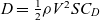$D = \frac{1}{2}\rho {V^2}S{C_D}$ , where $D$ is drag force. In the red-coloured section of the boundary, this reference area reduction is such that enables the airplane to increase speed while total drag force (and hence, the required thrust) is decreasing. The airplane’s turn rate reduces as it decreases sideslip angle. It keeps increasing speed and reducing sideslip until it enters coordinated turn (zero sideslip), and from that point, bank angle decreases until the airplane is in non-sideslipping wings level rectilinear flight at top of the flight envelope (end of the thrust saturation boundary).

Stall speed increases as the aircraft increases bank angle:

(21) \begin{equation}{\raise0.7ex\hbox{$L$} \!\mathord{\left/{\vphantom {L W}}\right.}\!\lower0.7ex\hbox{$W$}} = {\raise0.7ex\hbox{$1$} \!\mathord{\left/{\vphantom {1 {cos\phi }}}\right.}\!\lower0.7ex\hbox{${cos\phi }$}} = n\end{equation}

(22) \begin{equation}{V_S} = \sqrt {{\raise0.7ex\hbox{${2L}$} \!\mathord{\left/{\vphantom {{2L} {\rho {C_{{L_{max}}}}S}}}\right.}\!\lower0.7ex\hbox{${\rho {C_{{L_{max}}}}S}$}}} = \sqrt {{\raise0.7ex\hbox{${2nW}$} \!\mathord{\left/{\vphantom {{2nW} {\rho {C_{{L_{max}}}}S}}}\right.}\!\lower0.7ex\hbox{${\rho {C_{{L_{max}}}}S}$}}} \end{equation}

(23) \begin{equation}{V_{{S_t}}} = \sqrt n {V_{{S_0}}} = {\raise0.7ex\hbox{$1$} \!\mathord{\left/{\vphantom {1 {\sqrt {cos\phi } }}}\right.}\!\lower0.7ex\hbox{${\sqrt {cos\phi } }$}}{V_{{S_0}}}\end{equation}

where, $n,\;W,\;{V_{{S_t}}},\;{V_{{S_0}}}$ are load factor, weight, turning maneuver stall speed, and wings level rectilinear flight stall speed. Stall speed is proportional to load factor as presented in (22), (23), and load factor increases with roll angle; as shown in (21). Stall speed increase can be seen in the stall boundary section of Figs. 5 and 7. However, instead of being gradual, such increase is in the form of $V$ -constant sections.

$V$ -constant sections in the stall boundary of the unimpaired flight envelope shown in Fig. 5 are generally due to numeric round-off error and resolution increment size of the $V$ range (1knot). In fact, the speed increases gradually (according to (23)) and if the increment size is reduced significantly (e.g. to 0.1 knots), these stepwise constant sections would be eliminated and replaced by a curve of boundary trim points. However, this would considerably increase the computational cost, which is unnecessary as a sufficiently accurate flight envelope boundary has already been estimated with the current increment size.

The effect of these $V$ -constant sections can be seen as “sawtooths” in the zoomed-in-plot of Fig. 6. In Fig. 6, these sawtooths can be described as increase in the angle-of-attack in $V$ -constant sections, and sudden decrease in the angle-of-attack between the $V$ -constant sections. As the aircraft banks, lift vector inclines, hence there is lesser lift available to balance the weight. Therefore, the angle-of-attack must be increased to prevent loss of altitude. This is the reason for the increase of angle-of-attack in $V$ -constant sections. In each $V$ -constant section, the angle-of-attack increases until it reaches the critical value. So, the extra lift required to prevent loss of altitude cannot be provided by increasing angle-of-attack anymore. At this point, the required lift is generated by increasing speed, and the current $V$ -constant section changes to the next $V$ -constant section. Between the $V$ -constant sections; where extra required lift is provided by an increase in the speed, there would be lesser need in the angle-of-attack, and that is why the angle-of-attack decreases between the $V$ -constant sections.

$\phi $ -constant and $\beta $ -constant thrust-required curves are plotted in Fig. 11. Usually in texts and articles, only $\phi = 0$ thrust-required curve is plotted along with thrust-available curve. However, in this research, “ $\phi = 30,\;\;\beta $ -constant” curves have been additionally calculated and plotted for various amounts of the sideslip angle to show that by moving along the trim points of the flight envelope boundary, the required thrust increases and the boundary trim points pass through $\beta $ -constant curves. For better realisation, these curves are shown in the unimpaired flight envelope boundary in Fig. 12. These curves are confined by the stall boundary/aileron saturation boundary on one side and the thrust saturation boundary on the other side.

Figure 12.

$\boldsymbol\beta $ -constant curves in unimpaired flight envelope at sea level and zero flight path angle.

There are segments in the green-coloured boundary of Fig. 9, where one trim point has saturated aileron of 20°, whilst in the next few trim points, the trim value of aileron deflection is slightly lower than 20°. In these segments, speed increases with constant turn rate, which increases the aileron effectiveness, and hence lesser aileron (<20°) is needed for the same amount of turn rate. However, this does not mean that the airplane can access the adjacent trim point if it uses full 20° aileron deflection. This is due to the fact that $\dot \psi $ increments of 0.2deg/s have been used and the adjacent trim point $\left( {\dot \psi + 0.2} \right)$ requires aileron deflection of greater than 20°.

Similar behaviour is seen in the thrust saturation boundary of Fig. 11. There are segments in which a trim point has 100% throttle setting whilst the next few ones do not fully lie on the thrust-available curve. Again, the reason is the increment size of turn rate. At such trim points, if the turn rate is increased by 0.2deg/s, the required thrust would be more than the available thrust, and in order to stay on the thrust-available curve, the turn rate should be increased by less than 0.2deg/s, which is not available due to the utilised $\dot \psi $ increments. However, after increasing speed by 3 or 4 knots, the next trim point lies on the thrust-available curve again, which is resulted by simultaneous increase in speed and decrease in available thrust. A sample segment is chosen in Fig. 11 to demonstrate this behaviour. Zoomed-in-plot of this segment shows five trim points, which the first and the last ones are placed on the thrust-available curve, whereas the other three are beneath the curve. As shown in Table 6, these three trim points require greater than available amounts of thrust to become their adjacent trim points (same $V$ , $\dot \psi + 0.2$ ).

Table 6

Thrust required for three sample trim points

Despite the fact that left aileron (positive ${\delta _a}$ ) is needed to initiate a roll to the left, it is shown in Figs. 9 and 10 that right aileron (negative ${\delta _a}$ ) and left rudder (positive ${\delta _r}$ ) are required to perform a left turn (negative $\phi $ ) maneuver. The reason that right aileron is needed to maintain the bank angle constant during the left coordinated turn, can be explained as following: As the airplane banks to the left, an adverse yawing moment is generated which yaws the airplane to the right while the airplane is rolling to the left. To counteract this yawing moment, some left rudder input is required, which its exact amount is primarily dependent on yaw damping derivative of the airplane. Due to roll-yaw coupling, this rudder input produces some right increment in the rolling moment; however, it is not enough to compensate for the effects of flight path curvature. Hence, some right aileron input is also required^{(Reference Philips45)}.

Unimpaired flight envelopes of GTM at four different altitudes of sea level, 10,000ft., 20,000ft., and 30,000ft. are presented in Fig. 13. It can be seen that flight envelope contracts as the altitude increases. To understand why flight envelope shrinks, the boundary needs to be investigated.

Figure 13.

Unimpaired flight envelopes at zero flight path angle and various altitudes.

According to (22), it is evident that by increasing altitude; stall speed increases too, which is due to decrease in the air density. Hence, the magenta-coloured segment of the boundary (the stall boundary) goes up with the increase in altitude.

As shown in Fig. 14, increasing altitude results in reduction of engines’ available thrust. This leads to lesser maximum speed $\left( {{V_{max}}} \right)$ at the higher altitude. This is why the red-coloured segment of the boundary (thrust saturation boundary), contracts and lowers with the increase in altitude.

As the altitude increases, the aileron saturation boundary (green-coloured segment) gets smaller and the aileron saturates sooner (at smaller turn rates), until 30,000ft. where the aileron saturation boundary completely vanishes. To understand why this happens, the result of an investigation done on the intersection trim point of stall boundary and aileron saturation boundary; at different altitudes, is presented in Table 7.

Table 7

Intersection trim point status at various altitudes

Figure 14.

Thrust-available – thrust-required curves for various flight path angles and different altitudes.

Based on Table 7, at sea level the aileron is saturated whilst thrust is far from saturation. However, by increasing altitude, the point where the stall boundary ends and the aileron saturates will have lesser distance from thrust saturation. Therefore, the green segment of the boundary becomes smaller. As the aircraft arrives at 30,000ft., there is no distance left between the thrust saturation boundary and the end of the stall boundary. So, thrust is saturated long before the aileron saturates ( ${\delta _a}\;$ = −13.36°) and the green segment disappears.

Also due to decrease in the air density, aileron effectiveness reduces with increase in the altitude. Hence more rudder input is required to achieve the same turn rate of the previous altitude, which means more aileron deflection is needed to maintain the bank angle constant at 30°, and consequently the aileron saturates sooner.

As seen in Fig. 13, there is a sudden indent on each side of the thrust saturation boundary of the 30,000ft. flight envelope. Source of these indents is in the thrust-required curve of the GTM. There are few slight ups and downs at the bottom of all thrust-required curves of the GTM (see Fig. 14), which are due to the aerodynamic coefficients in the aero datasets. At 30,000ft., the distance between thrust-required curve and thrust-available curve is such limited that for some trim points with speeds corresponding to the mentioned ups, the amount of the required thrust for many turn rates fall beyond the thrust-available curve. Hence, to be able to trim the aircraft at mentioned speeds, the turn rate needs to be reduced significantly.

Figure 15 shows unimpaired flight envelopes for various flight path angles at sea level. As expected, the stall boundary and the aileron saturation boundary are almost at the same location for different flight path angles. This is due to the fact that flight path angle has no significant effect on stall speed value or saturation of aileron.

Figure 15.

Unimpaired flight envelopes at sea level and various flight path angles.

However, thrust saturation boundary shifts down by increasing flight path angle, which means lesser thrust and lesser maximum speed $\left( {{V_{max}}} \right)$ are available as the flight path angle increases. This is completely in compliance with the following equation:

(24) \begin{equation}{T_R} = W\gamma + \frac{1}{2}\rho {V^2}S{C_{{D_0}}} + {\raise0.7ex\hbox{${2K{W^2}}$} \!\mathord{\left/{\vphantom {{2K{W^2}} {\rho {V^2}Sco{s^2}\phi }}}\right.}\!\lower0.7ex\hbox{${\rho {V^2}Sco{s^2}\phi }$}}\end{equation}

in which, ${T_R}$ and $K$ are required thrust and drag polar parameter, respectively^{(Reference McClamroch46)}. According to (24), the required thrust increases with increase in flight path angle. This is also evident in Fig. 14. On the other hand, thrust available curve is the same for different flight path angles, because they are all considered at the same altitude. Consequently, ${V_{max}}$ reduces as flight path angle increases.

It is important to note that at 30,000ft., the airplane can fly only up to 2° flight path angles. In the other words, there are no climbing steady maneuvers feasible for the GTM with $\gamma > 2$ at 30,000ft. This is because the thrust-available curve has dropped significantly, and there is very limited thrust available at this altitude. Also, thrust-required curve has elevated with each incremental increase of flight path angle, as in (24). For flight path angles greater than 2°, all required thrust values are higher than all available thrust values.

The maximum available flight path angle can be computed from the following equation:

(25) \begin{equation}{\gamma _{max}} = \frac{{T_{max}^S}}{W}{\left( {\frac{\rho }{{{\rho ^S}}}} \right)^m} - 2cos\phi \sqrt {K{C_{{D_0}}}} \end{equation}

where $T_{max}^S$ and ${\rho ^S}$ are maximum engines’ thrust and air density at sea level. Using (25) at 30,000ft. also results in 2° maximum flight path angle.

By the way, it should be noted that the GTM flies at lower altitudes than the full-scale aircraft^{(Reference Ouellette, Raghavan, Patil and Kapania47)}, as it is a sub-scale remotely-piloted air vehicle designed to fly at low altitudes only (line of sight). However, the MFEs were also evaluated at 20,000ft. and 30,000ft. using the GTM’s MATLAB^® – Simulink^® model for the purpose of demonstrating and evaluating the envelope variations. So, the 2° limit of flight path angles does not exist for the full-scale aircraft at 30,000ft., and it can achieve higher flight path angles at this altitude.

It is also of great importance and interest to evaluate the V-n diagram of the GTM at sea level with different levels of thrust impairment. The upper curved-line boundary in this GTM’s V-n diagram corresponds to the stall saturation boundary at the bottom of the GTM’s unimpaired maneuvering flight envelope at sea level and zero flight path angle. Also, the upper horizontal-line boundary of the V-n diagram usually presents the maximum positive load factor (bank angle) an aircraft can achieve before structural failures. This maximum positive load factor is specified by the FAR25 for the transport category aircraft. For instance, a B747-400 has a maximum load factor of 2.5 corresponding to a maximum bank angle of 66.5°. Since GTM is a subscale model, it better fits the FAR23 normal category aircraft (nonacrobatic) for which the bank angle is limited to 60°. Hence, in the calculations of the V-n diagram, the structural limit for the GTM’s bank angle has been considered as 60°. Such a limit on the bank angle allows for higher turn rates than the imposed 30° bank constraint. It should be noted that despite providing access to higher turn rates, this structural bank limit is not the value technically being used in steady state maneuvers or non-transient maneuvers which require holding bank angle for a period of time, and as mentioned in Section 3.4.1, in studies where the employed model is a jet transport it is common to impose a bank constraint much lower than the structural limit.

However, in order to calculate the upper horizontal-line boundary of the V-n diagram, the maneuvering flight envelope of the unimpaired GTM at sea level and zero flight path angle must be re-evaluated with the 60° bank constraint in effect. Figures 16 and 17 present the evaluated maneuvering flight envelope of the unimpaired GTM and the corresponding variation of the stall boundary trim points’ bank angle with total speed, respectively.

Figure 16.

Unimpaired flight envelope at sea level and zero flight path angle (60° bank constraint).

Figure 17.

Variation of the stall boundary trim points’ bank angle with total speed.

The black-coloured curves on sides of the envelope in Fig. 16 are composed of boundary trim points with ±60° bank and no sideslip. For the sake of comparison, the ±30° constant bank – no sideslip curves are plotted on the same envelope. The 30° bank curve is also shown in Fig. 12 with the same green colour.

It is important to note the difference between the re-evaluated unimpaired envelope presented above and the other unimpaired flight envelope presented and investigated previously (i.e. Fig. 12). While both envelopes contain the same coordinated maneuvers in the area confined by the 30° bank green curves, further trim points outside this area in Fig. 12 have non-zero sideslip angles with 30° bank angle due to the imposed 30° bank constraint, whereas all trim points in the envelope presented in Fig. 16 correspond to coordinated maneuvers due to the imposed zero sideslip constraint.

Based on the unimpaired flight envelope boundaries shown in Fig. 16, the V-n diagram of the GTM is as shown in Fig. 18. According to the presented explanations, the magenta-coloured curve and black-coloured horizontal line in the V-n diagram correspond to the magenta-coloured stall boundary and black-coloured 60° bank boundary in the unimpaired envelope presented above. The corresponding load factor values along the aforementioned curve and horizontal line have been calculated using the boundary trim points’ bank angle value (the $\phi - V$ plot presented above) and equation (20).

Figure 18.

V-n diagram of the GTM at sea level.

It should be noted that the exact values of the negative limit maneuvering load factor ( $ - {n_{max}}$ ), negative stall speed ( ${V_{{S_{NEG}}}}$ ), cruising speed ( ${V_C}$ ), and dive speed ( ${V_D}$ ) must be provided by the designer which in the case of the GTM, such information is not provided in the GTM-DesignSim or the related documents, and the regulations only provide relations for the minimum possible values of ( $ - {n_{max}}$ ), ( ${V_C}$ ), and ( ${V_D}$ ). Thus, the approximate values for these parameters have been calculated for the presented V-n diagram as following: the absolute value of the $ - {n_{max}}$ should not be less than 40% of the maximum positive load factor for the normal and commuter category aircraft according to the FAR23, this yields a minimum value of −0.8. It is also common to consider it −1 for the transport category aircraft, hence, in this research, $ - {n_{max}}$ has been set to −1.

Since most wing airfoils have positive camber, their positive stall angles are often higher than the absolute values of their negative stall angles and the absolute value for the typical negative maximum lift coefficient is about 50% of the positive maximum lift coefficient. Therefore, the typical negative stall speed ( ${V_{{S_{NEG}}}}$ ) is about 40% greater than the positive stall speed ( ${V_S}$ )^{(Reference FAR48)}. The exact value for ( ${V_S}$ ) is 57.5 knots which results in 80.5 knots negative stall speed ( ${V_{{S_{NEG}}}}$ ).

FAR23 defines the minimum design cruising speed ${V_C}$ as $33\sqrt {W/S} $ and the minimum ${V_D}$ as 1.4 ${V_C}$ , but no relation for exact value of the ${V_D}$ itself. However, according to^{(Reference Sadraey49)}, dive speed $\left( {{V_D}} \right)$ is often greater than the maximum speed $\left( {{V_{max}}} \right)$ which is slightly higher than the aircraft design cruising speed $\left( {{V_C}} \right)$ , where ${V_{max}}$ is intersection of thrust-available and thrust-required curves. Also, based on regulations “ ${V_C}$ should not exceed the maximum speed in level flight at maximum continuous power, for the corresponding altitude”^{(Reference FAR48)}. Hence,

(26) \begin{equation}{V_C} \le {V_{max}} < {V_D}\end{equation}

Therefore, in this study it has been assumed that the above equation holds for the level flight. According to the presented unimpaired flight envelope, ${V_{max}}$ is 176 knots (thrust saturation boundary), consequently, approximate values of 170 knots for ${V_C}$ and (1.4 ${V_C} = $ 238 knots) for ${V_D}$ have been considered.

In Fig. 18, the vertical red dashed lines demonstrate the corresponding maximum speeds for the unimpaired case ( ${V_{max}}$ ) and different levels of thrust impairment ( ${V_{90\% }}$ , ${V_{80\% }}$ , ${V_{70\% }}$ , and ${V_{60\% }}$ ).

5.2 Impaired flight envelopes

In this section, the aim is to investigate the effect of control surface failure on the MFE. Hence, several impaired flight envelopes are plotted at a number of flight conditions for comparison purposes, and variation of their boundaries with respect to each other are analysed.

Figure 19.

Rudder restriction cases at sea level and $\gamma \text{=}\, \text{--}\, \text{5}^\circ $ .

Figure 20.

Rudder restriction cases at 30,000ft. and $\gamma \text{= 0}^\circ $ .

Figure 21.

Rudder restriction cases at 30,000ft. and $\gamma \text{= 0}^\circ $ .

5.2.1 Rudder restriction cases

By analysing the boundaries of the impaired flight envelopes shown in Figs. 19–21, it is concluded that in the rudder restriction cases, the right side of the flight envelope boundary corresponds to the lower limit of the rudder deflection angle, whereas the left side of the boundary corresponds to the upper limit. The reason is that right deflection of rudder (negative ${\delta _r}$ ) causes positive yawing moment (and its corresponding adverse roll), which initiates turn to the right (positive turn rates). On the other hand, when rudder deflects to the left (positive ${\delta _r}$ ), the generated negative yawing moment results in negative turn rates (turn to the left).

As shown in the presented figures, when rudder deflection is restricted, flight envelope contracts and the impaired boundary separates from the boundary of the unimpaired case.

This separation occurs at that side of the flight envelope which its corresponding limit is lower than that of the unimpaired case (e.g. the limit being 10° instead of 30°). For instance, in Fig. 19, all of the three impaired cases $\left[ { - 30,\;20} \right]$ , $\left[ { - 30,10} \right]$ , and $\left[ { - 30,0} \right]$ – have right boundaries attached to the right boundary of the unimpaired flight envelope. Because their lower limit of the rudder deflection angle is the same as the lower limit in the unimpaired aircraft (i.e. −30°). However, their upper limits are lower than 30°, so their left boundaries are separated from the left boundary of the unimpaired case, where the amount of separation (distance between their left boundary and the unimpaired boundary) is proportional to the value of their upper limit. As the upper limit value lowers, the failure gets severe (i.e. control restriction tightens), so the impaired boundary retreats more inside the unimpaired flight envelope and distances more from the unimpaired boundary.

Another outcome of the performed analysis is shown in Tables 8 and 9 in which ✓ represents the existence of difference between the corresponding impaired boundary and the unimpaired boundary, whereas ✗ means no difference.

Table 8

[−20, UL]/[LL, 20] difference with the unimpaired boundary

Table 9

[−10, UL]/[LL, 10] difference with the unimpaired boundary

Table 8 shows at which altitude and flight path angle, the right boundary of the impaired flight envelope in [−20, UL] case (or the left boundary in [LL, 20] case) is the same as the right (or left) boundary of the unimpaired flight envelope, and at which altitude and flight path angle, it is separated.

According to Table 8, as flight path angle and altitude increase, it is more likely that the unimpaired and impaired cases have the same corresponding boundary. That is because by increasing altitude or flight path angle, the unimpaired flight envelope contracts and thrust saturation boundary becomes more dominant (see Figs. 13 and 15). This contraction and domination leads to smaller amounts of required rudder deflection angle at the boundaries of the unimpaired flight envelope, because further trim points are infeasible due to lack of thrust. So when the limit of the restricted rudder is bigger than the required deflection values of the unimpaired boundary trim points, the impaired aircraft can be trimmed at the unimpaired boundary trim points even with the restricted rudder. Similar explanation is applicable to Table 9.

For example, at sea level and zero flight path angle, the maximum rudder deflection angle used in unimpaired boundary trim points is ±26° (Fig. 11); however, this value reduces to ±7° at 30,000ft. because trim maneuvers which require rudder deflection of more than ±7° are infeasible due to thrust saturation. Therefore any rudder restriction failure in which the restricted lower or upper limit is beyond ±7°, impose no restriction on airplane’s maneuverability at 30,000ft. (Table 9).

In Fig. 20, flight envelope of the impaired case [−30, 10] is the same as the unimpaired case [−30, 30], because the furthest trim point on the boundary of the unimpaired flight envelope requires less than 10° rudder deflection, hence the restriction has no effect (Table 9). This is also the reason that the unimpaired flight envelope is not visible in that figure. It is completely covered by the impaired flight envelopes [−30, 10] and [−30, 20].

The impaired case [−20, 10] in Fig. 21 corresponds to both of the Tables 8 and 9. Neither the lower limit boundary nor the upper limit boundary has any difference with the unimpaired flight envelope boundary.

It should be noted that the symmetry of the estimated flight envelopes (described in the beginning of this section), results in validity of Table 8 for both the [−20, UL] and [LL, 20] cases. With the same reasoning, Table 9 is valid for both the [−10, UL] and [LL, 10] cases.

It can be seen that in most cases, top (thrust saturation boundary) and bottom (stall boundary) of the impaired flight envelope are attached to top and bottom of the unimpaired flight envelope, except for that side of the boundary which is separated. In such cases, the deflection range of the impaired rudder includes 0° deflection, which means that the aircraft is able to perform non-sideslipping maneuver (β = 0). However, there are cases in which impaired rudder deflection range excludes 0° deflection. In these cases there are either positive rudder inputs available or negative rudder inputs available. Thus the aircraft is always sideslipped ( $\beta \ne 0)$ , which yields in persistent extra drag force. Such drag increases required thrust, which in turn leads to lower maximum speed and higher minimum speed. These cases are called “high drag” in this research. It is evident in the presented figures that for the high drag cases, always top of the impaired boundary and sometimes (if the restriction is highly tightened) bottom of the impaired boundary separates from the unimpaired boundary. For instance in Fig. 19, [−30, −10] and [−30, −20] are both high drag cases.

Figures 19–21 are three instances among numerous comparison plots generated within this study. Due to the space limitations of the paper, the rest of the comparison plots are provided in Ref. (Reference Norouzi, Kosari and Sabour43).

It is worthy to check the validity of the results of the previous unimpaired flight envelope analysis in the impaired cases too. Therefore, three impaired cases are chosen and plotted in different altitudes and flight path angles (Figs. 22–24).

Figure 22.

Rudder restriction [−10, 0] at zero flight path angle.

Figure 23.

Rudder restriction [−20, 0] at 10,000ft.

Figure 24.

Rudder restriction [−30, 10] at $\gamma \text{= -- 5}^\circ $ .

In Fig. 22, impaired flight envelopes shrink as expected with the increase in altitude, which is consistent with Fig. 13. Figure 23 demonstrates lowering of the thrust saturation boundary with increase in the flight path angle, which is due to increase in the required thrust. Same behaviour is seen in Fig. 15 for the unimpaired cases. In Fig. 24, despite the contraction of the impaired flight envelope, maximum speed is the same for different altitudes. A phenomenon completely in compliance with Fig. 14, which shows that in $\gamma = - 5^\circ $ , maximum speed does not change with the variation in altitude.

5.2.2 Aileron restriction cases

General rules inferred from the rudder restriction cases are valid for the aileron restriction cases too, except for few details changed. Lower limit of the aileron deflection angle corresponds to the left side of the flight envelope boundary, because right aileron (negative ${\delta _a}$ ) incurs a positive rolling moment which is followed by an adverse negative yawing moment which makes left turns (negative turn rates) more accessible. Consequently, upper limit corresponds to the right side of the flight envelope boundary.

As in the rudder restriction cases, restricted aileron failures which do not include the 0° deflection angle are always sideslipped ( $\beta \ne 0)$ and endure permanent extra drag force. For example, the impaired case [−20, −10] in Fig. 25 is a high drag case.

Figure 25.

Aileron restriction cases at sea level and $\gamma \text{=0}^\circ $ .

Figure 26.

Aileron restriction cases at 30,000ft. and $\gamma \text{=0}^\circ $ .

Figure 27.

Aileron restriction [−10, 10] at $\gamma \text{=0}^\circ $ .

Figure 28.

Aileron restriction [−20, 0] at sea level.

Figure 29.

Rudder jamming cases at sea level and $\gamma \text{= 0}^\circ $ .

Figure 30.

Rudder jamming cases at 10,000ft. and $\gamma \text{= -- 5}^\circ $ .

Figure 31.

Intersection of flight envelopes at sea level and $\gamma \text{= 5}^\circ $ .

Figure 32.

Intersection of flight envelopes at sea level and $ \text{=0}^\circ $ .

In contrast to the rudder restriction cases, there is no impaired aileron flight envelope boundary that is the same as the unimpaired boundary. For instance, in Fig. 26, the right side of the boundary of aileron impaired case [−10, 10] and the left side of the boundary of the impaired case [−10, 0] are very close to the corresponding unimpaired boundary, however they have very slight differences. This means that in all aileron restriction failures, the effect of the unavailability of part of the aileron deflection range is more dominant than the thrust saturation.

Eventually, flight envelope variation of the impaired case [−10, 10] with the increase in altitude, and flight envelope variation of the impaired case [−20, 0] with the increase in flight path angle are demonstrated in Figs. 27 and 28, respectively. As expected, the variations are consistent with Figs. 13 and 15.

5.2.2.1 Rudder jamming cases

Figures 29 and 30 present maneuvering flight envelopes for a number of rudder jamming failure cases. These figures show that when the rudder is jammed at a positive deflection angle, the aircraft tends to turn left. That is because positive rudder deflection (left rudder) incurs negative yawing moment. Also, it can be seen that as the rudder jamming angle increases (failure gets severe), flight envelopes are more drifted to the left, i.e. left turning maneuvers with higher turn rates become accessible whilst turning maneuvers with lower turn rates become infeasible.

This behaviour can be explained as following:

In the unimpaired case, when the bank angle reaches its maximum value (according to the imposed 30° bank constraint), the airplane can still achieve higher turn rates by performing slipping turn. To do so, simultaneous opposite rudder and aileron inputs are used to yaw the aircraft whilst maintaining the bank angle at 30°. However, in the impaired cases there are no rudder inputs available when the aircraft reaches maximum allowable bank angle (because the rudder is jammed), so it is impossible for the airplane to perform slipping turn and maintain bank angle. Thus further turn rates and trim points are infeasible.

Also it is evident that the rudder jammed airplane has permanent sideslip $\left( {\beta \ne 0} \right)$ , which yields in shifting the flight envelopes of the impaired cases to the left (more negative turn rates) in the $\phi - \dot \psi $ plot. The more the rudder jammed angle, the more the shifting, and hence the more drifted is the impaired flight envelope.

By investigating the maneuvering flight envelopes of the rudder jamming cases and comparing them with the restricted rudder flight envelopes, the following conclusion is drawn:

Each jammed rudder flight envelope is the intersection of two restricted rudder flight envelopes. This statement can be shown as below:

(27) \begin{equation}J\left[ X \right] = R\left[ {LL,{\rm{\;}}X} \right] \cap R\left[ {X,UL} \right]\end{equation}

where $J$ denotes jamming, $R$ denotes restriction, and $X$ is the jammed rudder angle. For instance, maneuvering flight envelope of aircraft with jammed rudder at +20° is composed of trim points that are available in both of the flight envelopes of the restricted rudder cases [−30°, +20°] and [+20°, +30°]. This is shown in Fig. 31. Also in Fig. 32, it is presented that the maneuvering flight envelope of the aircraft with jammed rudder at +10° is the intersection of the flight envelopes of the restriction cases [−20°, +10°] and [+10°, +20°].

5.2.4 Aileron jamming cases

Figures 33 and 34 present maneuvering flight envelopes for a number of aileron jamming failure cases. As can be seen, when aileron is jammed at a positive value, the aircraft tends to turn to the right. That is because left aileron (positive ${\delta _a}$ ) incurs a negative rolling moment which is followed by an adverse positive yawing moment which makes right turns (positive turn rates) more accessible.

Figure 33.

Aileron jamming cases at sea level and $\gamma \text{= -- 5}^\circ $ .

Figure 34.

Aileron jamming cases at 10,000ft. and $\gamma \text{= 0}^\circ $ .

As the aileron jamming angle increases, maneuvering flight envelopes are more drifted to the right, so higher turn rates become feasible whilst lower turn rates become inaccessible.

Similar to the intersection rule inferred from the rudder jamming failures exists for the aileron jamming cases. Each jammed aileron flight envelope is the intersection of two restricted aileron flight envelopes. Figure 35 demonstrates an instance where the maneuvering flight envelope of the impaired aircraft with jammed aileron at 0° is the intersection of the flight envelopes of the restriction cases [−20°, 0°] and [0°, +10°].

Figure 35.

Intersection of flight envelopes at sea level and $\gamma \text{= -- 5}^\circ $ .