NOMENCLATURE
- α
path slope parameter
- θ1,θ2
fibre-angle functions
- β
path curvature parameter
- ϑ1, ϑ2, . . .
design variables (fibre-angles)
- δα
load-drop due to load path asymmetry
- h
total shell-wall thickness
- δβ
load-drop due to instability
- k
shell curvature parameter l 2y/Rh
- Δ
end-shortening
- lx
shell axial length
- Δc, Δ1, Δ2
constants in the end-shortening series
- ly
shell circumferential arc-length
- f
objective function
- R
shell internal radius
- γ
buckling mode interaction angle
- u
displacement vector
- kr
relative post-buckling stiffness
- u0
pre-buckling displacements
- λ
axial force magnitude
- v
linear buckling mode
- λc
critical buckling load
- w
quadratic corrector
- λQIc
critical quasi-isotropic buckling load
- x, y
surface co-ordinates
- r
perturbation radius
- c
null-space coefficient vector
 $\tilde{\theta }$
path tangent angle
- f
nodal force vector
- Aij
laminate membrane stiffness constants
- K0
pre-buckling stiffness matrix
- Dij
laminate bending stiffness constants
- K1
geometric stiffness matrix
- E 11, E 22, G 12
lamina local elastic moduli
- Kb
buckling stiffness matrix
- ν12
lamina local Poisson’s ratio
- ni
null-space basis vectors
- ν
isotropic Poisson’s ratio
- N
orthogonality matrix
- t
lamina thickness
- P
total potential energy functional
- θ
stacking sequence
- u, v, w
nodal displacement vectors
1.0 INTRODUCTION
Circular cylinders are well known for exhibiting dramatic collapse under axial compression. Their poor post-buckling behaviour has been shown to be due to instability of the initial buckling mode(Reference Koiter1) and the presence of a post-buckled configuration having a significantly smaller load than the critical value(Reference vonKármán and Tsien2). A direct consequence of the instability is an extreme sensitivity of the buckling load to imperfection in the surface geometry, materials and loading conditions. Linear buckling loads calculated based on perfect cylindrical geometries and loading may deviate significantly from those of the real structure. At certain values of the radius-to-thickness ratio, R/h, the NASA design code(Reference Peterson, Seide and Weingarten3) suggests a ‘knock-down’ of the linear results of as much as 60%. The tendency, therefore, is to over-design shells to account for any uncertainties in the design calculations.
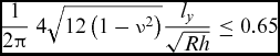
Conditions required for unstable post-bucking have been determined for a number of shell configurations. Koiter(Reference Koiter4) calculated the limiting values of internal radius R, wall-thickness h and width ly of isotropic curved panels under pure axial compression. He showed that stable behaviour corresponds to satisfaction of the inequality:
 $$\begin{equation}
\frac{1}{2\pi }\; 4\sqrt{12\left(1-\nu ^{2}\right)}\frac{l_{y}}{\sqrt{Rh}}\le 0.65
\end{equation}$$
where ν is Poisson’s ratio. Assuming h to be small compared with the other dimensions, satisfaction of Equation (1) constrains the radius to relatively large values compared with the panel width. Only a small amount of curvature, therefore, is required to produce unstable behaviour.
The situation is not greatly improved in the case of composite shells. Khot and Venkayya(Reference Khot and Venkayya5) calculated axial tangent stiffnesses of cylinders having stacking sequences in the families [ ± θ, 0]s and [ ± θ, 90]s. The laminates were made from glass- and boron-reinforced epoxy lamina. Here, an asymptotic perturbation approach was used to compute the initial post-buckling response. The results showed that in all cases (i.e. with all combinations of lamina material, stacking-sequence and angle θ) the shells were unstable.
Pope(Reference Pope6) calculated the tangent stiffness of curved sandwich panels using an incremental approach. The presence of orthotropy in the shell-wall was shown to augment the inequality in Equation (1), delaying the unstable behaviour to smaller values of R. The limiting values of panel curvature, however, were still significantly smaller than those required for a complete cylinder.
A traditional means of stabilising cylinders and reducing their imperfection sensitivity is to attach stiffening elements (e.g. see Fig. 1(a)). The principle here is that the attachment of structural elements with stable post-buckling responses increases the stability of the overall structure. This idea has been explored by Mang et al(Reference Mang, Schranz and Mackenzie-Helnwein8) and Schranz et al(Reference Schranz, Krenn and Mang9) in the context of unstable bar and shell structures. In the case of shells, the stringers are designed to avoid the formation of a global buckling pattern by confining significant radial displacements to the curved skins. Design codes generally suggest smaller reductions of linear results (i.e. smaller knock-downs) for stiffened shells due to their reduced imperfection sensitivity (a summary of the knock-down factors may be found in Ref. 10). The obvious drawback to such a design is the added mass associated with the stringers and their attachment.
Composite shells designs for reduced imperfection sensitivity. (a) Axially stiffened(Reference Bisagni and Cordisco7), (b) Variable-stiffness (curvilinear fibres)(Reference Wu, Stanford, Hrinda, Wang, Martin and Kim11), (c) Hybrid glass-carbon-reinforced epoxy(Reference Burgueño, Hu, Heeringa and Lajnef12), (d) ‘Wavy’ shell design.(Reference Ning and Pellegrino13)

Recently, researchers have been exploring alternative means of stabilising cylinders by using advanced materials and manufacturing techniques. Wu et al(Reference Wu, Stanford, Hrinda, Wang, Martin and Kim11) produced cylinders with reinforcement orientations which varied in the surface co-ordinates. The shells were designed with a circumferential fibre-angle variation, resulting in two adjacent regions of high membrane and bending stiffness, and two of high in-plane shear and twisting stiffness (see Fig. 1(b)). Under axial compression, large axial membrane stresses developed in the regions of high membrane stiffness, resulting in a highly localised buckle and a post-buckled state. The shells exhibited a relatively low imperfection sensitivity and a reserve of stiffness in the post-buckling regime.
The variable-stiffness (VS) theme was continued by Burgueño et al(Reference Burgueño, Hu, Heeringa and Lajnef12) who performed experiments and computational analyses of glass-fibre reinforced polymer (GFRP) shells having patterns of additional uni-directional carbon fibre reinforced polymer (CFRP). Figure 1(c) shows a typical example of their designs. Three orientations of the carbon bracing were considered: 0/90, ± 30 and ± 45. In all cases, buckling was not followed by a catastrophic collapse, rather a series of small drops in load, before a final, more significant collapse. These results are interesting because they show a potential for tailoring a cylinder’s post-buckling behaviour. The authors did not, however, make any general conclusions with regard to the effect of stiffness variations on the observed buckling behaviour.
An alternative design philosophy, aimed at reducing imperfection sensitivity explicitly, was investigated by Ning and Pellegrino(Reference Ning and Pellegrino13). Building on the work of Jullien and Araar(Reference Jullien and Araar14), the cylindrical cross-section was designed with a ‘wavy’ pattern. Its precise shape was tailored to minimise the knock-down factor (see Fig. 1(d)) based on linear finite-element buckling analyses. The resulting designs were tested and found to fail at loads very near to the buckling load. However, due to the small specimen size and the relatively small radii of the ‘wavy’ shell-wall, the failure occurred due to material failure.
In a VS composite design, it is assumed that the orientation of the reinforcing fibres are functions of the structure’s surface co-ordinates. Such an effect may be made possible, in practice, by defining the reinforcement using curvilinear paths, which is in contrast to traditional straight fibre laminates. By designing in this way, it is possible to tailor a structure’s mechanical behaviour locally. In the present work, the idea of imparting an inherent post-buckling stability on cylindrical shells is investigated. An attempt is made to break Koiter’s inequality (1) by designing the shell with a VS laminate. To achieve this aim, an asymptotic post-buckling model of a curved panel under axial compression has been produced, based on initial post-buckling theory(Reference Koiter1). This model was used to compute the tangent stiffness of the post-buckling path which was subsequently maximised with respect to a set of reference fibre-angles, which defined continuous fibre-angle functions (in terms of the surface coordinates).
First, an overview of the asymptotic model and a derivation of the key stability parameters are derived. Next, the variable angle-tow (VAT) design space is defined and the details of the optimisation are described. Optimised straight-fibre designs are presented first and are compared with quasi-isotropic designs. The results are compared with non-linear finite-element analysis solutions for validation purposes. The optimised VAT shells are then presented and compared with the straight-fibre designs. Finally, we compare the asymptotic VAT models with finite-element models and explain the mechanisms behind the novel post-buckling behaviour.
2.0 THEORETICAL ANALYSIS
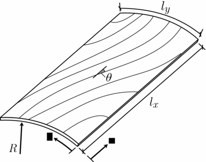
Consider the panel shown in Fig. 2. It has axial length lx, circumferential arc-length ly, an internal radius of curvature R, and a total laminate thickness h. The latter three parameters are encapsulated by the non-dimensional curvature parameter k = l 2y/Rh, which is one eighth of the panel bulge-to-thickness ratio. The shell-wall comprises a CFRP laminate which is assumed to have fibre-orientations varying as functions of the surface co-ordinates x and y. Tangential displacements in the axial and circumferential directions are denoted u and v, and radial displacements are denoted w. When combined, these fields make up the displacement vector  $\boldsymbol{u}\in \mathbb {R}^{3}$.
Panel geometry showing curvilinear fibre paths and co-ordinate directions.
The panel is loaded under pure axial compression by a force of magnitude λ. Its ends (i.e. the boundaries at x = 0 and lx) are assumed to be simply supported (i.e. w = Mx = 0) and to be uniformly displaced in the x-direction (i.e. ∂u/∂y = 0). Furthermore, the sides (i.e. the boundaries at y = 0 and ly) are assumed to be simply supported (i.e. w = My = 0) and are free to expand (i.e. Ny = 0).
2.1 Asymptotic post-buckling analysis
Koiter’s(Reference Koiter1) asymptotic method is employed to solve the post-buckling problem. Its advantage, over path following or time-integration methods, is its computational efficiency. Under the assumption that only solutions in the neighbourhood of the critical buckling load are required, the non-linear post-buckling problem may be solved with relatively few integration operations. It has been applied to many stability problems (examples of its implementation may be found in Refs 4 and 15-19). A short overview of its application is given here.
In the pre-buckling regime, the structure is assumed to behave linearly, that is, the displacements are assumed to be given by
 $$\begin{equation}
\boldsymbol{u}=\lambda \boldsymbol{u}_{0}
\end{equation}$$
where the vector field u0 is the displacement vector resulting from a unit load. This linear relationship holds until the well-known critical load, λc, is reached, at which point an adjacent state is present. Displacements of the structure in the adjacent state are written as a power series, in terms of the scalar perturbation radius, designated r. That is:
 $$\begin{equation}
\boldsymbol{u}=\lambda \boldsymbol{u}_{0}+\boldsymbol{v}r+\boldsymbol{w}r^{2}+O\left(r^{3}\right)
\end{equation}$$
where v is the first-order buckling mode and w is a quadratic corrector. The first-order displacement vector is the eigenmode corresponding to the buckling eigenvalue λc. The quadratic corrector, w, is required to maintain equilibrium of the structure at finite values of r.
Despite the tendency of shells to have multiple coalesced buckling loads, it was found (through comparisons with non-linear finite-element solutions) that un-coupled post-buckling analyses were sufficient for capturing the behaviour of the structures considered. Post-buckling analyses (i.e. the calculation of w) were carried out independently for the first two eigenmodes.
Given the displacement fields defined by Equation (3) it is possible to use the principle of stationary potential energy to compute a power series for the load in terms of r. Substituting the displacements into the total potential energy and making the result stationary in the r-direction gives:
 $$\begin{equation}
\lambda =\lambda _{c}+\alpha r+\beta r^{2}+O\left(r^{3}\right)
\end{equation}$$
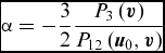
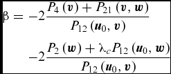
where α is the path slope and β is the path curvature. The parameters α and β are dimensional forms of Koiter’s a and b imperfection sensitivity parameters (a = α/λc and b = β/λc).
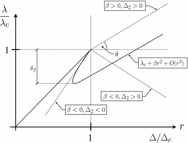
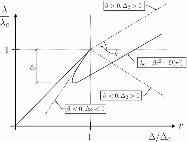
Paths having various values of α and β are shown in Fig. 3. The slope and curvature are represented by the coefficients of the odd and even parts of the function λ, respectively. A structure having a non-zero slope has at least one unstable path (i.e. reducing in load) emanating from its critical point. The curvature is a measure of the structure’s stability at larger values of the perturbation radius. By examining Equation (4), it is clear that a structure having a negative curvature is inherently unstable.
Load paths showing the contributions of the slope, α, and the curvature, β.
One possibility is a structure having a non-zero slope and a positive curvature. Such a structure is stable for relatively large values of r but which exhibits a drop in load near the critical point. The magnitude of the load drop may be calculated by considering the stationary value of the load λ in the radial direction r. Such a stationary point corresponds to a drop in load:
 $$\begin{equation}
\delta _{\alpha }=\frac{\alpha ^{2}}{4\beta }
\end{equation}$$
The drop in load δα is associated purely with the load-asymmetry of the linear buckling mode v. It is also possible for drops in load and subsequent restabilisation to occur due to higher-order effects. For example, a long curved panel with simply supported sides will generally have a symmetric buckling mode (i.e. α = 0) and a negative path-curvature (i.e. β < 0). Immediately after buckling, instability (associated with β) results in a load-drop and a loss of stiffness. As further end-shortening is applied load is re-distributed to the boundaries (where radial displacements cannot occur) and the structure restabilises. In order to differentiate between the latter effect and those associated with asymmetry, the load-drop associated with β is termed δβ (see Fig. 4).
Axial force–end-shortening paths for post-buckled shells, having three combinations of Δ2 and β.
Using the series for the load parameter (4) and the displacements (3) it is possible to calculate the post-buckled axial stiffness. We define the end-shortening at finite-values of the perturbation radius as:
 $$\begin{equation}
\Delta =\Delta _{c}+\Delta _{1}r+\Delta _{2}r^{2}
\end{equation}$$
where
 $$\begin{equation}
\Delta _{c}=\lambda _{c}\boldsymbol{u}_{0}\left(l_{x},y\right)
\end{equation}$$\\
 $$\begin{equation}
\Delta _{1}=\alpha \boldsymbol{u}_{0}\left(l_{x},y\right)+\boldsymbol{v}\left(l_{x},y\right)
\end{equation}$$\\
 $$\begin{equation}
\Delta _{2}=\beta \boldsymbol{u}_{0}\left(l_{x},y\right)+\boldsymbol{w}\left(l_{x},y\right.)
\end{equation}$$
In order to quantify the panel stiffness in the post-buckling regime, we make use of the path angle, denoted  $\tilde{\theta }$. This has been used previously by Khot and Venkayya(Reference Khot and Venkayya5) in the context of complete circular cylinders. It is a necessary measure instead of a simple stiffness parameter, due to the possibility of path reversal. To calculate $\tilde{\theta }$, we must first calculate the tangent stiffness in a normalised force-displacement plane (ignoring the asymmetry parameter α). This is given by
 $$\begin{equation}
k_{r}=\left.\frac{\partial }{\partial r}\left(\frac{\lambda }{\lambda _{c}}\right)\bigg/\frac{\partial }{\partial r}\left(\frac{\Delta }{\Delta _{c}}\right)\right|_{\alpha =0}=\frac{\beta }{\Delta _{2}}
\end{equation}$$
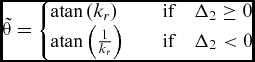
where kr is the tangent stiffness relative to the pre-buckling path. Noting that the displacement parameter Δ2 may be negative (i.e. the path may reverse), we define the path angle $\tilde{\theta }$ in the following piecewise form:
 $$\begin{equation*}
\tilde{\theta }=\left\lbrace \begin{array}{@{}l@{\quad }l@{}}\text{atan}\left(k_{r}\right) & \quad \text{if}\quad \Delta _{2}\ge 0\\
\text{atan}\left(\frac{1}{k_{r}}\right) & \quad \text{if}\quad \Delta _{2}<0 \end{array}\right.
\end{equation*}$$
A depiction of the path angle, $\tilde{\theta }$, is given in Fig. 4 with various combinations of Δ2 and β. The range of $\tilde{\theta }$ is typically 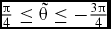 $\frac{\pi }{4}\le \tilde{\theta }\le -\frac{3\pi }{4}$ radian. At its maximum value the post-buckled path is identical to the pre-buckling path (this is unlikely to occur in reality) and at its minimum value the pre-buckling path is reversed.
In order to calculate the various path parameters, a set of linear variational problems must be solved for the displacement fields u0, v and w. This procedure has previously been accomplished by finite-element discretisation(Reference Lanzo and Garcea16), analytical solution via conversion into the strong form(Reference van der Heijden18), Galerkin reduction(Reference Koiter4) and the Generalised Differential Quadrature (GDQ) method(Reference White, Raju and Weaver19).
In the present work, the differentiation and integration required to approximate the total potential energy functional is accomplished by a combined GDQ-Generalised Integral Quadrature (GIQ) numerical method. Details of the calculation of the displacement fields and the load parameters may be found in Appendix A.
3.0 OPTIMISATION
The objective of our optimisation study is to produce designs which are ‘well behaved’ in the post-buckling regime. A classic example of a well-behaved non-linear structure is a simply-supported von Kármán plate loaded in its plane. Here, the large transverse buckling displacements cause a redistribution of membrane stress to the stiff boundaries. The resulting post-buckled path is guaranteed to have  $\tilde{\theta }>0$ and δα = δβ = 0. With this in mind, the curved panels were optimised with the objective of maximising the path angle $\tilde{\theta }$. This was achieved by minimising the following objective function:
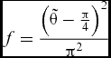 $$\begin{equation}
f=\frac{\left(\tilde{\theta }-\frac{\pi }{4}\right)^{2}}{\pi ^{2}}
\end{equation}$$
which varies parabolically from f(− 3π/4) = 1 to f(π/4) = 0.
Interestingly, it was not found necessary to include the path slope, α, into the objective function. In the case of constant stiffness shells, the buckling modes were sufficiently distributed that the load-path was approximately symmetric (i.e. the structure may be classified as quartic (Reference Salerno and Casciaro20)). The VS shells did have asymmetric buckling modes; however, non-linear finite-element analysis showed that the stable direction was significantly more attractive than the unstable direction. That is, the drop in load associated with the asymmetry, δα, did not correlate with Equation (5). This behaviour was found to be due to the presence of a bending deformation in the pre-buckling regime which had the same effect as a geometric imperfection. The matter is discussed further in Section 4.2.2.
3.1 Fibre-angle variation
We use VAT composite laminates defined by the following stacking sequence:
 $$\begin{equation}
\boldsymbol{\theta }=\left[\left(\pm \theta _{1}\left(x,y\right)\right)_{2},\left(\pm \theta _{2}\left(x,y\right)\right)_{2}\right]_{s}
\end{equation}$$
where the functions θ1(x, y) and θ2(x, y) are the outer and inner fibre-angle functions, respectively. This stacking sequence was chosen to (a) eliminate any extension-bend and extension-twist coupling (to encourage a pure membrane pre-buckling state) and (b) to take advantage of any beneficial zeroth- vs second-moment of area effects (i.e. to impart greater design freedoms).
Two-dimensional linear interpolation functions, with symmetry about the lines x = lx/2 and y = ly/2, were chosen to define the two angle functions. The interpolated fibre-angles (i.e. the design variables) are designated ϑ1 − ϑ4 for the outer ply and ϑ5 − ϑ8 (for the inner ply). The locations of the interpolation points are shown in Fig. 7, in the results section. The values of the eight design parameters were constrained to be members of the set:
 $$\begin{equation}
\vartheta _{i}\in \left\lbrace 0,5,10,15,\dots ,90\right\rbrace
\end{equation}$$
In order to form a comparison, the following constant-stiffness stacking sequence is also defined:
 $$\begin{equation}
\boldsymbol{\theta }=\left[\pm \vartheta _{1},\pm \vartheta _{2},\pm \vartheta _{3},\pm \vartheta {}_{4}\right]_{s}
\end{equation}$$
3.2 Optimisation algorithm
The post-buckling design space of VS panels is, in general, discontinuous and non-convex. This makes the use of gradient-based non-linear minimisation methods inefficient. A genetic algorithm was, therefore, employed to search for the global minimum. This method is based on evolution by natural selection and is very common in engineering optimisation problems (a good reference may be found in Ref. 21). The particular algorithm used in the study was the genetic algorithm toolbox found in MATLAB(22).
In each optimisation, generations (having populations of 50 panels) were iterated until the change in the average value of the objective functions f (i.e. for the entire population) was smaller than 1 × 10⁻⁷. Each new generation was populated by crossover children (with a crossover fraction equal to 0.8), elite children (2 per generation) and mutants (with a mutant fraction of 0.2).
As a check, each optimisation run was repeated at least once in order to make sure that the global optimum had been found. In the event that the result was significantly different, a third optimisation was performed and the best design of the three was used.
4.0 RESULTS AND DISCUSSION
In this section, we present numerical results of the optimisation studies. In all cases, the panel has dimensions lx = 2500 mm, ly = 500 mm and h = 2.1 mm (i.e. 16 plies). The material properties of the CFRP lamina are given in Table 1.
Lamina elastic properties

In contrast to a buckling optimisation, in which paths having the smallest buckling mode are selected, our optimisation studies have been conducted on the basis of the least stable path (in terms of $\tilde{\theta }$). This is defined as the path of steepest decent (for  $\tilde{\theta }<0$) or the path of weakest ascent (for $\tilde{\theta }>0$).
Optimal results, calculated using our own asymptotic code, were compared with non-linear finite-element simulations. The static arc-length (Riks) implementation in Abaqus 6.12(23) was used to model the shells’ unstable post-buckling behaviour with meshes of S4R elements. In each case the mesh density was based on convergence of the buckling eigenvalues. The VS finite-element models were produced using the Abaqus/Python scripting interface.
4.1 Constant stiffness laminates
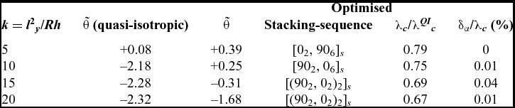
Shells having constant-stiffness laminates were optimised first. The stacking sequence defined by Equation (14) was optimised with the objective of maximising $\tilde{\theta }$ (i.e. by minimising f). The results are shown in Table 2 and are compared with those for shells having the quasi-isotropic stacking sequence [(0, 90, ±45)2]s.
Optimal laminates for shells for maximising $\tilde{\theta }$ (radian)
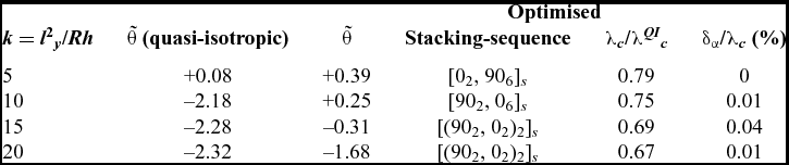
Shells having low curvatures have stable post-buckling paths. As the curvature parameter k is increased, the quasi-isotropic (QI) panel’s stability decreases and the transition from stable to unstable behaviour occurs with k in the range 5 ⩽ k ⩽ 10. This result is in agreement with the findings of both Koiter(Reference Koiter4) and Pope(Reference Pope6). It is worth noting that, according to our analysis, a flat QI plate of these dimensions would have a value of $\tilde{\theta }$ equal to approximately +0.48 rad.
The optimised designs, which in general have laminates with various combinations of zero and ninety degree plies, have improved stability compared with the QI case. Here, the transition from stable to un-stable occurs for k in the range 10 ⩽ k ⩽ 15. Interestingly, it appears that a side effect of improving the panel’s post-buckling behaviour is a reduction in the buckling load (20–30% for the panels considered). The same effect is observed in flat composite plates (for example, see Ref. 24) and is due to the conflicting requirements of the bending-dominated buckling with the membrane dominated post-buckling regimes.
4.1.1 Finite-element results
In order to validate the results shown in Table 2, finite-element analyses were performed for each of the optimised and quasi-isotropic designs. In order to calculate a bifurcated path using the arc-length method, the meshes were perturbed by adding a small (max amplitude h/1000) component of the buckling mode displacements to the un-deformed geometry. The results of these are shown in Fig. 5 and are normalised with respect to their own buckling load and critical end-shortening.
Normalised force vs end-shortening finite-element (Riks) results for constant-stiffness shells: optimised vs quasi-isotropic.
Results for the least curved shell (see Fig. 5(a)) confirm that both the quasi-isotropic and the optimised designs are both stable, and that the latter has a larger relative axial stiffness. As the curvature increases, the finite-element results match the data trends presented in Table 2. The quasi-isotropic shell having k = 10 exhibits a complete reversal of its equilibrium path at the critical point, with an initial buckling mode having four half-waves in the x-direction switching to one with three. The optimised shell of the same curvature, on the other hand, has a plate-like response. In this case, the number of half-waves in the x-direction is fixed at five for the entire post-buckling path. The quasi-isotropic shell having the largest curvature shows a path reversal and a significant drop in load (δβ/λc ≈ 30%) at the point of bifurcation. It is emphasised that this drop in load is due to the negative path curvature and higher-order restabilisation, not load asymmetry. The optimised shell of the same curvature exhibits an unstable post-buckling response but without a path reversal (i.e.  $\tilde{\theta }>-\pi /2$).
4.2 Variable stiffness laminates
Section 4.1 demonstrated the stabilising effects of laminate orthotropy. It is clear, however, that its potential is limited to relatively small curvatures. In this section, the potential for inherently stable shells with curvilinear fibres is explored.
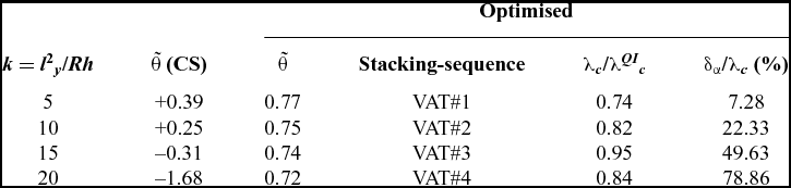
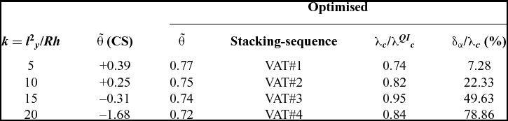
The path angle, $\tilde{\theta }$, was maximised with respect to the design variables ϑ1 − ϑ8. The results of these optimisation studies are presented in Table 3 and are compared with the optimised solutions for the constant-stiffness panels (see Table 2). The values of the design variables corresponding to each solution are shown in Table 4.
Optimal laminates for shells with curvilinear fibres for maximising post-buckling stability
VAT ply fibre-angle definitions (degrees)

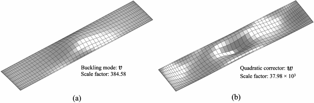
The results show a striking improvement in the value of $\tilde{\theta }$ compared with the corresponding constant stiffness (CS) panels. In the most highly curved case the drop in stiffness associated with buckling is 4.51% (i.e. kr = 0.88). This result indicates that for at least one value of  $\text{sign}\left(r\right)$, the structure is stable and is relatively unaffected by buckling (in terms of axial force). Buckling and post-buckling modes for the optimised panel having k = 20 are shown in Fig. 6. The fibre-angle functions are also plotted for this panel in Fig. 7.
Modes for a panel with k = 20 and the fibre-angle function corresponding to ‘VAT#4’.
Fibre-angle tangent plots for the lay-up ‘VAT#4’.
The first-order buckling mode v (see Fig. 6(a)) has a localised bulge and a circumferential contraction in the panel’s centre. It is possible that the localisation is a consequence of the orientation of the fibres in this region. In the case of a flat plate, the function for the critical buckling stress is proportional to  $\sqrt{D_{11}D_{22}}$ and (D 12 + 2D 66). It follows that, as the former term is the geometric mean of principal stiffnesses and its value is relatively unaffected by stacking sequence changes, the buckling stress is increased by maximising the latter. In the case of the ‘VAT#4’ shell, this term is minimum in the panel’s centre and largest at the locations (lx/4, y) and (3lx/4, y). As such a localised buckling half wave is promoted and ‘trapped’ at the centre.
The numerical results in Table 3 show a clear trend of increasing load drop δα with increasing curvature k for the optimised panels. The fact that a large drop in load is associated with the modes shown in Fig. 6 is a result of the mode v consisting of a single radial half-wave. The effect of the parity of the wave numbers of v on the path slope for curved panels is explained in Ref. 19.
4.2.1 Finite-element simulations
The optimal panels shown in Table 3 were analysed using finite-element path-following methods. The resulting axial-compression vs end-shortening curves are shown in Fig. 8.
Force vs end-shortening finite-element (Riks) results for VS shells: optimised vs quasi-isotropic.
The finite-element results are in good agreement with the asymptotic predictions. All of the optimised shells were unaffected by buckling in terms of axial stiffness and axial force. This result is due to (a) the distribution of membrane stress in the pre-buckling regime and (b) the localised radial displacements in the panel’s centre (i.e. at x = lx). The membrane stress-resultant, Nx, for the panel having k = 20 is plotted in Fig. 9. At axial loads corresponding to λ/λc = 0.1, the magnitude of Nx is largest along the panel’s sides (i.e. at y = 0 and ly). This effect occurs due to the distribution of axial membrane stiffness. At y = ly/2, the fibres are oriented in the circumferential direction giving the laminate a relatively small local axial stiffness. At the sides, however, the fibres are oriented in the axial direction giving this region a relatively large axial stiffness. The load path through the shell, therefore, is primarily along the side regions.
Membrane stress resultant (Nx) plots in the pre- and post-buckling regimes.
As the axial force increases into the post-buckling range, the radial displacement pattern consists of a single half-wave in each direction (see Fig. 6). At axial loads corresponding to λ/λc = 1.3, the distribution of Nx has changed little compared with its pre-buckling form. This lack of load redistribution explains the retention of axial stiffness throughout the loading.
Interestingly, the asymmetry of the buckling modes, which is manifested in the parameter δα, was not observed in the finite-element analysis results. Perturbing the un-deformed mesh with a component of the linear buckling mode (using a range of positive and negative scaling factors) did not result in an unstable equilibrium path. In fact, an imperfection larger in magnitude than the wall thickness was required to produce inward radial displacements in the post-buckling regime. This was found to be due to the development of bending moments and radial displacements in the pre-buckling regime. This effect is discussed further in the next section.
4.2.2 Effects of pre-buckling bending moments
Given the panel’s boundary conditions and its symmetric stacking sequence, the development of pre-buckling radial displacements is counter-intuitive. In fact, it is purely a consequence of the stiffness variations employed. This deduction becomes evident when considering Donnell’s(Reference Donnell26) membrane equilibrium equation in the x-direction:
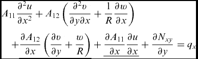 $$\begin{eqnarray*}
&&A_{11}\frac{\partial ^{2}u}{\partial x^{2}}+A_{12}\left(\frac{\partial ^{2}v}{\partial y\partial x}+\frac{1}{R}\frac{\partial w}{\partial x}\right)\\
&&\quad +\underline{\frac{\partial A_{12}}{\partial x}\left(\frac{\partial v}{\partial y}+\frac{w}{R}\right)}+\underline{\frac{\partial A_{11}}{\partial x}\frac{\partial u}{\partial x}}+\frac{\partial N_{xy}}{\partial y}=q_{x}
\end{eqnarray*}$$
where A 11 and A 12 are membrane stiffness constants and qx is a surface traction in the x-direction. The underlined terms are only present in VS structures. By inspection, it is clear that the presence of a differentiable stiffness variation in the x-direction produces new means of resisting surface tractions (in this case, by developing radial displacements). It is unsurprising, therefore, that the variation in stiffness has a non-trivial effect on a shell under axial loading.
Using the perfect cylindrical mesh the maximum radial displacements at the buckling load are of magnitude w/h = 1.4. These displacements occur in the panel’s centre where the axial membrane stresses are relatively small. A plot of the pre-buckling radial displacements is shown in Fig. 10. It is not surprising, therefore, that imposed imperfections have little effect on the buckling and post-buckling behaviour. The pre-buckling displacements result in the path corresponding to a positive (i.e. outward) radial bulge being highly attractive. This effect has been shown previously to occur in isotropic panels under combined loads (see Ref. 25).
Radial displacements w for the ‘VAT#4’ shell in the pre-buckling regime.
As the load is increased further, radial displacements grow rapidly. At an axial load corresponding to λ/λc = 1.3, they have magnitude w/h = 3. The final deformed shape has a long axial bulge similar in shape to that of the pre-buckling regime.
5.0 CONCLUSIONS
The potential of tailoring curved composite panels for inherent post-buckling stability has been investigated. An efficient model of panel post-buckling was produced using Koiter’s asymptotic theory and the methods of generalised differential and integral quadrature. This model was used with a genetic algorithm to maximise the panel’s post-buckling tangent stiffness.
Performance improvements were found for both straight and curved fibre composite panels. The best improvements, however, were seen for the latter. Designs were found having practically no degradation of axial stiffness in the post-buckling regime and displaying negligible drops in load.
Additional design drivers, such as stiffness and strength, were not taken into account during the optimisation process. In future work, multi-objective optimisations will be performed in order to find more practical stable shell designs.
ACKNOWLEDGEMENTS
The authors would like to acknowledge the Engineering and Physical Sciences Research Council for funding the Centre for Doctoral Training in Advanced Composites. Grant No. EP/G036772/1. This paper was first published at the 4th Aircraft Structural Design Conference of the Royal Aeronautical Society, Belfast, September 2014.
A NUMERICAL POST-BUCKLING ANALYSIS
In the following section, a brief outline of the methods used to solve to the panel post-buckling problems is given.
A.1 Variational equilibrium problems
The pre-buckling, buckling and quadratic-correction displacement fields are solutions to a set of linear variational problems. Using Koiter’s(Reference Koiter1,Reference van der Heijden18) notation, they may be written in the form:
 $$\begin{equation}
P_{11}\left(\boldsymbol{u}_{0},\boldsymbol{\xi }\right)=\boldsymbol{\xi }^{T}\boldsymbol{f}_{0}
\end{equation}$$
 $$\begin{equation}
P_{11}\left(\boldsymbol{v},\boldsymbol{\xi }\right)+\lambda _{c}P_{111}\left(\boldsymbol{u}_{0},\boldsymbol{v},\boldsymbol{\xi }\right)=0
\end{equation}$$
 $$\begin{equation}
P_{11}\left(\boldsymbol{w},\boldsymbol{\xi }\right)+\lambda _{c}P_{111}\left(\boldsymbol{u}_{0},\boldsymbol{w},\boldsymbol{\xi }\right)=P_{21}\left(\boldsymbol{v},\boldsymbol{\xi }\right)
\end{equation}$$
with
 $$\begin{equation}
P_{111}\left(\boldsymbol{u}_{0},\boldsymbol{w},\boldsymbol{v}\right)=0
\end{equation}$$
where P(u) is the total potential energy functional,  $\boldsymbol{f}_{0}\in \mathbb {R}^{3}$ is a pre-buckling force field, and
 $\boldsymbol{\xi }\in \mathscr {K}$ is the kinematically admissible displacement variation (
 $\mathscr {K}$ is the space of kinematically admissible displacements). The subscripts of P refer to terms in its multi-nomial expansionFootnote 1. In the present shell, the total potential energy is fourth-order in terms of the displacements u. It may be ordered into the power series:
 $$\begin{equation*}
P=P_{1}+P_{2}+P_{3}+P_{4}
\end{equation*}$$
An example of an expanded functional P 11 is defined by
 $$\begin{equation*}
P_{2}\left(\boldsymbol{u}_{1}+\boldsymbol{u}_{2}\right)=P_{2}\left(\boldsymbol{u}_{1}\right)+P_{11}\left(\boldsymbol{u}_{1},\boldsymbol{u}_{2}\right)+P_{2}\left(\boldsymbol{u}_{2}\right)
\end{equation*}$$
The total potential energy is the double integral of the strain energy density (due to displacements of the surface) with respect to the x and y co-ordinates. In the present work, the strain energy was calculated on the basis of the Sanders-Koiter(Reference Sanders27) strain-displacement relations. Integration and differentiation of the displacement fields necessary to write the total potential energy, and its various expanded terms, was accomplished using the global methods of GDQ and GIQ (see Ref. 28). Equations (15(a)) to (15(d)) were, therefore, transformed into the following linear algebraic equations:
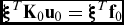 $$\begin{equation}
\boldsymbol{\xi }^{T}\mathbf {K}_{0}\mathbf {u}_{0}=\boldsymbol{\xi }^{T}\mathbf {f}_{0}
\end{equation}$$
 $$\begin{equation}
\boldsymbol{\xi }^{T}\left(\mathbf {K}_{0}+\lambda _{c}\mathbf {K}_{1}\right)\mathbf {v}=\boldsymbol{\xi }^{T}\mathbf {K}_{b}\mathbf {v}=\mathbf {0}
\end{equation}$$
 $$\begin{equation}
\boldsymbol{\xi }^{T}\mathbf {K}_{b}\mathbf {w}=\boldsymbol{\xi }^{T}\mathbf {f}_{2}\left(\mathbf {v}\right)
\end{equation}$$
and
 $$\begin{equation}
\mathbf {v}^{T}\mathbf {K}_{1}\mathbf {w}=\mathbf {0}
\end{equation}$$
where ξ(ξ) is the nodal form of ξ, K0 is the stiffness matrix calculated in the stress-free state, K1 is a geometric stiffness matrix, Kb is the tangent stiffness matrix at the buckling load, f2(v) is the post-buckling nodal force vector, and u0, v and w are the nodal forms of u0, v and w. Many alternative methods of discretising the variational problems are possible. For example, Lanzo et al(Reference Lanzo, Garcea and Casciaro15,Reference Lanzo and Garcea16) have used co-rotational finite-element formulations to form the various stiffness matrices given in Equations (16(a)) to (16(b)).
A.2 Solution methods
The pre-buckling problem (Equation (16(a))) may be solved by a standard matrix inversion operation for the displacement vector u0. Multi-point constraints required to maintain straight ends as well as rotational constraints at the panels ends were enforced via the penalty method. Additionally, fully constrained degrees of freedom were enforced by only considering variations, ξ, and displacements, u0, within the kinematically admissible vector subspace  $\mathscr {K}$ (i.e. by stiffness matrix condensation).
Equation (16(b)) is a linear eigenvalue problem in terms of the vector v and the critical load λc. In the present structures, it was found that two modes were often clustered in terms of their buckling loads. The first two modes are designated u1 and u2, and their corresponding loads are designated λc1 and λc2. The eigenvalue problem itself was solved using the eigs solver within MATLAB.
The post-buckling problem was solved using the following polar representation of the buckling modes:
 $$\begin{equation*}
\mathbf {v}=\mathbf {u}_{1}\cos \gamma +\mathbf {u}_{2}\sin \gamma
\end{equation*}$$
where γ is an interaction angle. Accounting for the possibility that λc1 and λc2 may be exactly equal, the following solution for w is sufficient for equilibrium:
 $$\begin{equation*}
\mathbf {w}=\mathbf {u}_{11}\cos ^{2}\gamma +\mathbf {u}_{12}\sin \gamma \cos \gamma +\mathbf {u}_{22}\sin ^{2}\gamma
\end{equation*}$$
where u11 and u22 are un-coupled post-buckling displacement vectors and u12 is a coupled post-buckling displacement vector. When the buckling loads are not exactly equal, the vector u12 is not required (for equilibrium) and the post-buckling solutions are given by the two independent paths having γ ∈ {0, π/2}.
In order to solve Equations (16(c)) and (16(d)) simultaneously, the search for w was carried out within the null-space of the row vector vTK1. Such a space is defined by
 $$\begin{equation}
N\left(\mathbf {v}^{T}\mathbf {K}_{1}\right)=c_{1}\mathbf {n}_{1}+c_{2}\mathbf {n}_{2}+\dots +c_{n}\mathbf {n}_{n}
\end{equation}$$
where ni are the the null-space basis vectors,  $c_{i}\in \mathbb {R}$ are the null-space coefficients and n is an integer one smaller than the number of displacement components. We denote the space defined by Equation (17) the orthogonal-space
 $\mathscr {O}$.
The post-buckling force-displacement equation may be modified for  $\mathbf {w}\in \mathscr {O}$ by introducing the coefficients ci as unknown variables. Substituting
 $$\begin{equation}
\mathbf {w}=\mathbf {N}\mathbf {c}
\end{equation}$$
into Equation (16(c)) gives:
 $$\begin{equation}
\boldsymbol{\xi }^{T}\left(\mathbf {K}_{b}\mathbf {N}\right)\mathbf {c}=\boldsymbol{\xi }\mathbf {f}_{2}\left(\gamma \right)
\end{equation}$$
where:
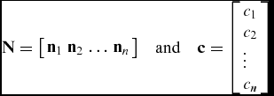 $$\begin{equation*}
\mathbf {N}={\left[$$\begin{array}{cccc}\mathbf {n}_{1} & \mathbf {n}_{2} & \dots & \mathbf {n}_{n}\end{array}$$\right]}\quad \text{and}\quad \mathbf {c}=\left[\begin{array}{l}c_{1}\\
c_{2}\\
\vdots \\
c_{n} \end{array}$$\right]
\end{equation*}$$
The matrix KbN is rectangular and, therefore, Equation (19) is unsolvable. The equation is rendered solvable (as it has been in many previous works, e.g. see Refs 4, 17 and 29) by only requiring the shell to be stationary with respect to variations in the orthogonal space, i.e.  $\boldsymbol{\xi }\in \mathscr {O}$. This is made possible by introducing the new variations:
 $$\begin{equation*}
\boldsymbol{\xi }=\mathbf {N}\boldsymbol{\xi }^{*}
\end{equation*}$$
where ξ*is the variational equivalent of c. Equation (19), therefore, becomes:
 $$\begin{equation}
\left(\mathbf {N}^{T}\mathbf {K}_{b}\mathbf {N}\right)\mathbf {c}=\mathbf {N}^{T}\mathbf {f}_{2}\left(\gamma \right)
\end{equation}$$
Equation (20) may be solved for c using standard matrix inversion (the matrix NTKbN is symmetric and invertible). The post-buckling displacement vector may be retrieved from the coefficients using Equation (18).
A.3 Path parameters
Equations for Koiter’s path constants have been derived in many publications (for example, see Refs 1, 4 and 19). They are written in terms of the potential energy functional components (i.e. P 2, P 3, . . .), and its various expansion terms (i.e. P 11, P 21, P 12, . . .). We quote them here as:
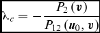 $$\begin{equation*}
\lambda _{c}=-\frac{P_{2}\left(\boldsymbol{v}\right)}{P_{12}\left(\boldsymbol{u}_{0},\boldsymbol{v}\right)}
\end{equation*}$$
 $$\begin{equation*}
\alpha =-\frac{3}{2}\frac{P_{3}\left(\boldsymbol{v}\right)}{P_{12}\left(\boldsymbol{u}_{0},\boldsymbol{v}\right)}
\end{equation*}$$
 $$\begin{eqnarray*}
\beta =-2\frac{P_{4}\left(\boldsymbol{v}\right)+P_{21}\left(\boldsymbol{v},\boldsymbol{w}\right)}{P_{12}\left(\boldsymbol{u}_{0},\boldsymbol{v}\right)}\\
&&-2\frac{P_{2}\left(\boldsymbol{w}\right)+\lambda _{c}P_{12}\left(\boldsymbol{u}_{0},\boldsymbol{w}\right)}{P_{12}\left(\boldsymbol{u}_{0},\boldsymbol{v}\right)}
\end{eqnarray*}$$
The integration and differentiation required to compute the path constants was accomplished using GDQ and GIQ.