





1. Introduction
The breaking of water waves is a fascinating phenomenon characterized by a number of dynamics – from phase mixing (e.g. Brocchini & Peregrine Reference Brocchini and Peregrine2001a,Reference Brocchini and Peregrineb; Brocchini Reference Brocchini2002) to turbulence generation (e.g. Melville, Veron & White Reference Melville, Veron and White2002) and dissipation (e.g. Grasso, Castelle & Ruessink Reference Grasso, Castelle and Ruessink2012) – and providing even more impacts on the nearshore region – from energy redistribution over various modes (e.g. Thornton & Guza Reference Thornton and Guza1986; Lippmann, Holman & Bowen Reference Lippmann, Holman and Bowen1997) to sediment transport (e.g. Beach & Sternberg Reference Beach and Sternberg1996), to open-sea mass-momentum-heat ocean–atmosphere exchange dynamics (e.g. Banner & Peregrine Reference Banner and Peregrine1993; Melville Reference Melville W1996; Duncan Reference Duncan2001).
For such reasons the modelling of wave breaking has seen ever-increasing interest and efforts, ranging from a suitable description of the fundamentals of the small-scale local mechanics to an efficient study of the large-scale dynamics. The optimal model would allow for inclusion of proper closures of the former into the equations used to represent the latter. This difficult exercise is being tackled via a number of approaches, which, from the historical viewpoint and focusing on the nearshore dynamics only, moved from the nonlinear shallow-water equations (e.g. Brocchini et al. Reference Brocchini, Bernetti, Mancinelli and Albertini2001) to Boussinesq-type models (e.g. Schäffer, Madsen & Deigaard Reference Schäffer, Madsen and Deigaard1993; Kennedy et al. Reference Kennedy, Chen, Kirby and Dalrymple2000), to large eddy simulation (LES) models (e.g. Christensen & Deigaard Reference Christensen and Deigaard2001) and to the most recent Reynolds-averaged Navier–Stokes (RANS) layer and non-hydrostatic models, using either algebraic (e.g. Smit, Zijlema & Stelling Reference Smit, Zijlema and Stelling2013) or PDE-type (e.g. Derakhti et al. Reference Derakhti, Kirby, Shi and Ma2016) closures for turbulence. The challenge is always the same – to combine accuracy in the description of the physics with a reasonably cheap computational cost in comparison to computational fluid dynamics simulations.
Our answer to the above challenge is through a model that incorporates both pioneering ideas and consolidated concepts to provide a robust, fairly accurate description of the evolution of breaking waves in the nearshore region. A pioneering element is a decomposition of the flow field that allows for the natural emergence of energy-dissipating terms through depth-integrated vorticity (e.g. Veeramony & Svendsen Reference Veeramony and Svendsen2000; Briganti et al. Reference Briganti, Musumeci, Bellotti, Brocchini and Foti2004; Antuono & Brocchini Reference Antuono and Brocchini2013; Antuono et al. Reference Antuono, Colicchio, Lugni, Greco and Brocchini2017) and the calculation of local three-dimensional (3-D) fields by means of perturbations to the depth-averaged flow. A more consolidated element is the use of the numerical techniques for quasi-hyperbolic equations to solve the core equations of the model, which are similar to the nonlinear shallow-water equations.
A fundamental innovative aspect of the proposed model, in comparison to the largest part of non-hydrostatic schemes, is the direct modelling of the vorticity dynamics. This is achieved through the application of smoothed particle hydrodynamics (SPH) type techniques, i.e. mollified operators, to solve for the 3-D vorticity evolution. In practice, this approach corresponds to the convolution of the vorticity equation with a positive compact-support weight function. The derived model is therefore expected to describe the vorticity dynamics at a length scale comparable with the dimension of the specific control volume identified by the weight function. Concerning the time scale, this is inherited from the depth-averaged model, since the dynamics is represented through a forced problem in which the vorticity is injected at the free surface as a consequence of wave breaking. Hence the free-surface motion and the specific forcing term at the free surface characterize the time scale of the vorticity dynamics. The specific expression for the vorticity injected at the free surface is borrowed from the work of Veeramony & Svendsen (Reference Veeramony and Svendsen2000) with slight modifications.
A further aspect deserving particular attention is the modelling of the turbulent viscosities in both vorticity and momentum equations. In fact, both LES and RANS approaches require too fine spatial/time discretizations and are therefore avoided in favour of a simpler representation. In particular, the turbulent viscosity in the vorticity equation is taken to depend on the reference spatial and time scales, and on the distance from the free surface, while an additional dependence on the enstrophy is used for the turbulent viscosity in the momentum equation.
Along with the definition of the wave-breaking model, we also introduce a slight modification of the breaking criterion proposed by Schäffer et al. (Reference Schäffer, Madsen and Deigaard1993) and later by Veeramony & Svendsen (Reference Veeramony and Svendsen2000). In that work, incipient breaking would occur for the local free-surface slope exceeding a given threshold.
In addition to this, we impose a consistency condition between the direction of the wave velocity and the gradient of the free-surface elevation. This avoids the detection of spurious breaking events as, for example, on the rear side of a steep advancing wave.
We underline that the implementation of the novel wave-breaking model has been done after a reshaping of the scheme described in Antuono et al. (Reference Antuono, Colicchio, Lugni, Greco and Brocchini2017, Reference Antuono, Valenza, Lugni and Colicchio2019). That was a preliminary step, necessary to improve the accuracy of the numerical model when simulating waves characterized by large steepness. The above-cited modifications are needed only for the numerical implementation, while the model equations are equivalent to Antuono et al. (Reference Antuono, Colicchio, Lugni, Greco and Brocchini2017, Reference Antuono, Valenza, Lugni and Colicchio2019) at the continuum. The present work is organized as follows. Section 2 summarizes the main changes in comparison to the previous versions, namely Antuono et al. (Reference Antuono, Colicchio, Lugni, Greco and Brocchini2017, Reference Antuono, Valenza, Lugni and Colicchio2019), then § 3 describes the wave-breaking model along with the details on the breaking criterion and choice of the turbulent viscosities. Section 4 illustrates both comparisons with some experimental data available in the literature and illustrations of the model applicability to 3-D conditions. Some brief conclusions close the paper.
2. The depth-semi-averaged model
The depth-semi-averaged model is made up of a subsystem of depth-averaged equations, similar to the Boussinesq-type models, and a Poisson equation for a depth-semi-averaged quantity  $\varUpsilon$ that is the integral of the vertical component of the velocity field from a given level up to the free-surface position. The latter equation represents the principal difference with respect to the existing non-hydrostatic models for coastal dynamics, since it replaces the Poisson equation for the pressure field that, in fact, never appears in the model. The solution for
 $\varUpsilon$ allows one to recover the velocity deviations from the depth-averaged velocity, and hence to compute all the nonlinear dispersive terms that cannot be represented through algebraic or differential expressions of the depth-averaged quantities. The key point of this representation is that both the forcing term and the boundary conditions of the Poisson equation for
 $\varUpsilon$ are known from the solution of the depth-averaged subsystem, and consequently no approximations are needed to close the model. In practice, the depth-semi-averaged model may be regarded as a rearrangement of the Euler equations or of the RANS equations, if suitable closures for the turbulent and vortical terms are provided. In any case, the use of depth-averaged and semi-averaged quantities suggests that the depth-semi-averaged model can be applied to describe wave dynamics in wide coastal regions at moderate computational costs.
In comparison with previous works (i.e. Antuono et al. Reference Antuono, Colicchio, Lugni, Greco and Brocchini2017, Reference Antuono, Valenza, Lugni and Colicchio2019), the terms containing the nonlinear dispersive contributions are here rearranged in a different manner. This is necessary to increase the robustness and stability of the numerical model when simulating steep waves. Specifically, the reformulation of the nonlinear dispersive terms is aimed at eliminating the presence of contributions proportional to the divergence of the depth-averaged velocity field, since these terms induce spurious oscillations when the wave steepness approaches the limit of breaking waves. This, which is purely a numerical problem, is a consequence of the depth-averaging procedure. Indeed, during the averaging over the depth, many terms in the momentum equation are rearranged by using the boundary condition along the free surface, since this allows for removal of boundary contributions in favour of integrated quantities (see, for example, Antuono & Brocchini Reference Antuono and Brocchini2013). For equations at the continuum, this procedure leads to perfectly equivalent expressions, but it may cause problems when the model is implemented numerically, since the continuity equation is obtained by using the same boundary condition along the free surface. This suggests that a sort of internal numerical resonance may occur between the continuity equation and the momentum equation, generating high-frequency spurious oscillations.
The rearranged model, which is equivalent at the continuum to the formulations shown in Antuono et al. (Reference Antuono, Colicchio, Lugni, Greco and Brocchini2017, Reference Antuono, Valenza, Lugni and Colicchio2019), reads
 \begin{equation} \left. \begin{array}{c@{}}
\displaystyle \dfrac{\partial d}{\partial t} +
\boldsymbol{\nabla} \boldsymbol{\cdot} ( \boldsymbol{U} d )
= 0 , \\ \begin{aligned} & \displaystyle \dfrac{\partial
M_{1}}{\partial t} + \left[\boldsymbol{U}
\boldsymbol{\cdot} \boldsymbol{M} - d U_2^{2} +
g\, \dfrac{d^{2}}{2} + f_{11} + D_{isp} \right]_x + [ U_1
U_2 d + f_{12} ]_y \\ & \quad = ( g d + p_b ) h_x +
\mathscr{T}_1 , \end{aligned}\\ \begin{aligned} &
\displaystyle \dfrac{\partial M_{2}}{\partial t} + [ U_1
U_2 d + f_{21} ]_x + \left[ \boldsymbol{U}
\boldsymbol{\cdot} \boldsymbol{M} - d U_1^{2} +
g\,\dfrac{d^{2}}{2} + f_{22} + D_{isp} \right]_y \\ & \quad
= ( g d + p_b ) h_y + \mathscr{T}_2 , \end{aligned}
\end{array} \right\} \end{equation}
where  $d = \eta +h$ is the total water depth,
 $\eta$ is the free surface elevation,
 $h$ is the seabed distance from the still-water level,
 $\boldsymbol {U} = (U_1, U_2)$ is the depth-averaged velocity, and
 $\boldsymbol {M} = (M_1, M_2)$ is the generalized mass flux, that is,
 \begin{equation} \boldsymbol{M} = \boldsymbol{Q} + \boldsymbol{\nabla} \left( \int_{{-}h}^{\eta} \varUpsilon \, \textrm{d}z \right) - \varUpsilon_B\,\boldsymbol{\nabla} h ,\quad \textrm{where } \varUpsilon = \int_{z}^{\eta} w \, \textrm{d}\zeta, \end{equation}
while  $\boldsymbol {Q} = \boldsymbol {U} d$ is the mass flux. The Poisson equation for the variable
 $\varUpsilon$ is described later, in § 2.2. Hereafter, the subscripts
 $F$ and
 $B$ indicate quantities evaluated at the free surface and along the bottom, respectively, and the symbol
 $\boldsymbol {\nabla }$ denotes the gradient operator in the two horizontal spatial directions, i.e.
 $\boldsymbol {\nabla } = (\partial /\partial x, \partial /\partial y)$.
The symbol  $\boldsymbol { \mathscr {T}} = ( \mathscr {T}_1, \mathscr {T}_2)$ represents the depth-averaged turbulent terms (which are described in the next subsection), while the remaining terms in the momentum fluxes are
 \begin{gather} f_{11} = \int_{{-}h}^{\eta} \delta u^{2} \, \textrm{d}z, \quad f_{12} = f_{21} = \int_{{-}h}^{\eta} \delta u\,\delta v \, \textrm{d}z, \quad f_{22} = \int_{{-}h}^{\eta} \delta v^{2} \, \textrm{d}z , \end{gather}
 $$\begin{gather} D_{isp} ={-} \frac{I \chi}{d} + \boldsymbol{\nabla} \boldsymbol{\cdot} \left( \int_{{-}h}^{\eta} (z+h) w\,\delta \boldsymbol{u} \, \textrm{d}z \right) - \int_{{-}h}^{\eta} w ( w + h_t + \delta \boldsymbol{u} \boldsymbol{\cdot} \boldsymbol{\nabla} h ) \, \textrm{d}z , \end{gather}$$
 $$\begin{gather}p_b ={-} \frac{\varUpsilon_B \chi}{d} + \boldsymbol{\nabla} \boldsymbol{\cdot} \left( \int_{{-}h}^{\eta} w\,\delta \boldsymbol{u} \, \textrm{d}z \right) + \boldsymbol{U} \boldsymbol{\cdot} \boldsymbol{\nabla} \varUpsilon_B , \quad I = \int_{{-}h}^{\eta} \varUpsilon \, \textrm{d}z , \end{gather}$$
 $$\begin{gather}\chi = h_t + w_F \, N_F^{2} - \left( \frac{\boldsymbol{M}}{d} + \boldsymbol{R}_F \right) \boldsymbol{\cdot} \boldsymbol{\nabla} \eta + \boldsymbol{U} \boldsymbol{\cdot} \boldsymbol{\nabla} d , \quad N_F = \sqrt{1 + \| \boldsymbol{\nabla} \eta \|^{2}} . \end{gather}$$
The velocity deviations  $\delta \boldsymbol {u} = (\delta u, \delta v)$ and the vertical velocity
 $w$ are obtained through knowledge of
 $\varUpsilon$ as
 \begin{equation} \delta \boldsymbol{u} ={-} \boldsymbol{\nabla} \varUpsilon + \frac{1}{d} \int_{{-}h}^{\eta} \boldsymbol{\nabla} \varUpsilon \, \textrm{d}z + \boldsymbol{R} , \quad w ={-} \varUpsilon_z, \end{equation}
and the term  $\boldsymbol {R}$ contains the vorticity contributions to the depth-semi-averaged model, namely
 \begin{equation} \boldsymbol{R} = \left( - \int_{z}^{\eta} \omega_2 \, \textrm{d}z + \frac{1}{d} \int_{{-}h}^{\eta} (z+h) \omega_2 \, \textrm{d}z , \int_{z}^{\eta} \omega_1 \, \textrm{d}z - \frac{1}{d} \int_{{-}h}^{\eta} (z+h) \omega_1 \, \textrm{d}z \right), \end{equation}
where  $\boldsymbol {\omega } = ( \omega _1 , \omega _2 , \omega _3 )$ is the vorticity field. Incidentally, we observe that the terms containing a double integration shown in Antuono et al. (Reference Antuono, Colicchio, Lugni, Greco and Brocchini2017) are here rearranged by using the identity
 \begin{equation} \int_{{-}h}^{\eta} \, \textrm{d}z \int_{z}^{\eta} f(\zeta) \, \textrm{d}\zeta = \int_{{-}h}^{\eta} (z+h)\,f(z) \, \textrm{d}z , \end{equation}
where  $f$ is a generic scalar function. This allows for a faster and more robust numerical implementation.
The numerical implementation of the above equations is essentially the same as described in Antuono et al. (Reference Antuono, Colicchio, Lugni, Greco and Brocchini2017). In brief, the numerical fluxes are evaluated through the MUSCL-Hancock scheme with the Harten–Lax–Van Leer approximate Riemann solver described by Toro (Reference Toro1999) and initially conceived for hyperbolic equations, while a fourth-order Adams–Bashforth–Moulton predictor/corrector scheme is used for the time integration. Finally, second-order central finite difference schemes are used to discretize the source terms. Minor changes are listed in Appendix A, along with details of the derivation of the present model from the previous versions, namely Antuono et al. (Reference Antuono, Colicchio, Lugni, Greco and Brocchini2017, Reference Antuono, Valenza, Lugni and Colicchio2019).
2.1. Depth-averaged turbulent terms
The turbulent terms are modelled through a Boussinesq closure. In particular, we need to specify only the expression for the turbulent viscosity  $\nu _T$ (eddy viscosity), since the turbulent kinetic energy
 $\kappa _T$ cancels out. This is a consequence of the fact that the depth-semi-averaged model does not contain the pressure field (which incorporates
 $\kappa _T$). Hence the Boussinesq closure reduces to
 \begin{equation} \langle { \hat{u}_i \hat{u}_j} \rangle ={-} 2 \nu_T {\boldsymbol{\mathsf{D}}}_{i j} , \quad i,j = 1,2,3, \end{equation}
where  ${\boldsymbol{\mathsf{D}}}_{i j}$ is the strain rate tensor. The whole expression for the pressure (i.e. including
 $\kappa _T$) is described in Antuono & Brocchini (Reference Antuono and Brocchini2013). That expression is useful for the evaluation of stresses along solid bodies, but it is superfluous for the description of the wave motion in the present scheme.
The depth-averaged turbulent terms read
 \begin{equation} \boldsymbol{ \mathscr{T}} ={-} \boldsymbol{\nabla} \boldsymbol{\cdot} {\boldsymbol{\mathsf{H}}} - \boldsymbol{\nabla} D_{isp}^{{\rm T}}+ p_b^{{\rm T}}\,\boldsymbol{\nabla} h + \boldsymbol{\tau}_B, \end{equation}
where
 $$\begin{gather} {\boldsymbol{\mathsf{H}}}_{11} = \int_{{-}h}^{\eta} \langle { \hat{u}^{2}} \rangle \, \textrm{d}z , \quad {\boldsymbol{\mathsf{H}}}_{22} = \int_{{-}h}^{\eta} \langle { \hat{v}^{2}} \rangle \, \textrm{d}z , \quad {\boldsymbol{\mathsf{H}}}_{12} = {\boldsymbol{\mathsf{H}}}_{21} = \int_{{-}h}^{\eta} \langle { \hat{u} \hat{v} } \rangle \, \textrm{d}z , \end{gather}$$
 $$\begin{gather} D_{isp}^{{\rm T}}= \boldsymbol{\nabla} \boldsymbol{\cdot} \left( \int_{{-}h}^{\eta} (z+h)\,\langle { \hat{w} \boldsymbol{\hat{u}} } \rangle \, \textrm{d}z \right) - \int_{{-}h}^{\eta} [ \langle {\hat{w}^{2}} \rangle + \langle { \hat{w} \boldsymbol{\hat{u}} } \rangle \boldsymbol{\cdot} \boldsymbol{\nabla} h ] \, \textrm{d}z , \end{gather}$$
 $$\begin{gather}p_b^{{\rm T}}= \boldsymbol{\nabla} \boldsymbol{\cdot} \left( \int_{{-}h}^{\eta} \langle { \hat{w} \boldsymbol{\hat{u}} } \rangle \, \textrm{d}z \right) , \end{gather}$$
while  $\boldsymbol {\tau }_B$ represents the stress along the seabed. The latter term is modelled using standard formulations available in the literature (e.g. simple quadratic drag laws) and represents the seabed friction. In any case, in all the test cases a free-slip condition is assumed along the bottom and
 $\boldsymbol {\tau }_B$ is therefore neglected.
The derivatives inside the turbulent terms are modelled through central second-order finite differences, and the integration over the fluid depth is undertaken using Simpson's rule.
2.2. The Poisson equation for  $\varUpsilon$

The solution for  $\varUpsilon$ is pivotal for the model because it is necessary to evaluate the velocity deviations
 $\delta \boldsymbol {u}$, the vertical velocity component
 $w$, and all the remaining terms in the horizontal momentum equation. This is achieved by solving a Poisson equation whose forcing term and boundary conditions come from the solution of the depth-averaged subsystem in equation (2.1). This part is identical to Antuono et al. (Reference Antuono, Colicchio, Lugni, Greco and Brocchini2017) and reads
 \begin{equation} \left. \begin{array}{c@{}} \displaystyle \Delta \varUpsilon + \varUpsilon_{z z} = \boldsymbol{\nabla} \boldsymbol{\cdot} \left(\dfrac{\boldsymbol{M}}{d} + \boldsymbol{R} \right),\\ \varUpsilon |_{z = \eta} = 0 , \\ \displaystyle \left. \dfrac{\partial \varUpsilon}{\partial n} \right|_{z ={-}h} ={-} \left. \left[ h_t + \left(\dfrac{\boldsymbol{M}}{d} + \boldsymbol{R}_B \right) \boldsymbol{\cdot} \boldsymbol{\nabla} h \right] \right/ N_B, \end{array}\right\} \end{equation}
where  $N_B = \sqrt {1 + \| \boldsymbol {\nabla } h \|^{2} }$, and
 $\Delta$ is the Laplacian operator in two spatial dimensions. Along the lateral boundary of the domain (e.g. walls, open boundary), a Neumann condition is assigned.
Before proceeding to the definition of the wave-breaking model, it is important to clarify some aspects of the representation of the vorticity field in the depth-semi-averaged model. As shown in the previous derivation, the third component of the vorticity field, namely  $\omega _3$, never appears in the present model. In fact, as proved in Appendix B, this component can be obtained from knowledge of the remaining quantities. Specifically, we find
 \begin{equation} \omega_3 = \boldsymbol{\nabla} \times \left(\frac{\boldsymbol{M}}{d} + \boldsymbol{R} \right). \end{equation}
As a consequence of the above result, the vorticity dynamics in the depth-semi-averaged model just relies on the evolution of the horizontal components, i.e.  $\omega _1$ and
 $\omega _2$. In practice, (2.16) is never used in numerical simulations, because it may lead to the generation of spurious vorticity in the fluid domain. In fact, in the absence of wave breaking and therefore of vorticity, (2.16) leads to
 $\boldsymbol {\nabla } \times (\boldsymbol {M}/d ) = 0$, which is only approximately satisfied in numerical simulations (especially when uneven bathymetries are considered). Consequently, (2.16) is avoided in favour of an explicit modelling of the vorticity dynamics. Incidentally, we observe that condition
 $\boldsymbol {\nabla } \times (\boldsymbol {M}/d ) = 0$ for irrotational flows is a consequence of the identity
 $\boldsymbol {M}/d = \boldsymbol {\nabla } \phi _F$, where
 $\phi _F$ is the velocity potential evaluated at the free surface (see Antuono et al. (Reference Antuono, Valenza, Lugni and Colicchio2019) for more details).
As a final remark, we point out that depth-averaged models cannot capture the actual interface between water and air during the wave-breaking process since this is not single-valued. In particular,  $\eta$ has to be regarded as a ‘mean’ elevation satisfying the mass conservation (see the sketch in figure 1). Hence it is not possible to describe fully the roller region generated by the breaking wave, and this has to be done in an ‘average’ way.
Sketch of (a) the rotational region (roller) generated by wave breaking (grey region) and (b) the free surface defined through it according to depth-averaged models.

The Poisson equation for  $\varUpsilon$ is discretized through second-order finite differences over stretched Cartesian grids. As described in Antuono & Brocchini (Reference Antuono and Brocchini2013), the Dirichlet condition
 $\varUpsilon = 0$ is imposed at the intersection points between the grid and the free-surface position by using finite-difference operators with variable grid spacing, while the diffusive boundary approach described in Li et al. (Reference Li, Lowengrub, Rätz and Voigt2009) is implemented for the assignment of the Neumann condition along the solid boundary.
3. The wave-breaking model
To complete the depth-semi-averaged equations, we need to estimate the vorticity field  $\boldsymbol {\omega }$ and the related rotational term
 $\boldsymbol {R}$. To this purpose, we define a wave-breaking model that is conceived to represent the vorticity injection at the free surface, caused by breaking events, and the subsequent evolution inside the fluid. The basic idea is to mollify the vorticity equation and obtain a model that is capable of describing the mean features of the vorticity evolution (including turbulence) at the spatial scales typical of the wave dynamics. The use of mollified operators is preferred to a central finite-difference scheme, because the proposed model is explicit in time. The proposed approach avoids the occurrence of spurious numerical oscillations that arise in those models and consequently leads to a more stable and accurate scheme.
Incidentally, we highlight that the approach based on the direct modelling of the vorticity equation is a natural choice in the framework of the depth-semi-averaged equations, since these rely intrinsically on the decomposition of the flow field in potential and rotational contributions (see, for example, Antuono & Brocchini Reference Antuono and Brocchini2013).
Let us consider the Reynolds-averaged vorticity equation in three dimensions:
 \begin{equation} \frac{ \partial \boldsymbol{\omega}}{\partial t} = \hat{\boldsymbol{\nabla}} \boldsymbol{\cdot} {\boldsymbol{\mathsf{F}}} + \hat{\boldsymbol{\nabla}} \boldsymbol{\cdot} {\boldsymbol{\mathsf{F}}}{}^{\rm T} + \nu\,\Delta \boldsymbol{\omega} , \end{equation}
where  $\boldsymbol {\omega } = \hat {\boldsymbol {\nabla }} \times \boldsymbol {u}$,
 $\hat {\boldsymbol {\nabla }}$ is the 3-D gradient operator,
 $\boldsymbol {u} = ( u, v, w)$ is the Reynolds-averaged velocity field,
 $\nu$ is the kinematic viscosity, and
 \begin{equation} {\boldsymbol{\mathsf{F}}} = ( \boldsymbol{u} \otimes \boldsymbol{\omega} - \boldsymbol{\omega} \otimes \boldsymbol{u} ) , \quad {\boldsymbol{\mathsf{F}}}{}^{\rm T} = \overline{ ( { {\boldsymbol{u}^{\prime}} } \otimes { {\boldsymbol{\omega}^{\prime}} } - { {\boldsymbol{\omega}^{\prime}} } \otimes { {\boldsymbol{u}^{\prime}} } ) }. \end{equation}
Here, the  ${}^{\prime}$ denote the turbulent quantities, the barred symbol indicates the Reynolds average, and the divergence operator is applied on the second component of the tensors
 ${\boldsymbol{\mathsf{F}}}$ and
 ${\boldsymbol{\mathsf{F}}}^\textrm {T}$. In analogy with the standard approaches in turbulence, we use a closure based on a Fick's diffusive law as follows:
 \begin{equation} {\boldsymbol{\mathsf{F}}}{}^{\rm T} = \tilde{\nu}_\omega \, \hat{\boldsymbol{\nabla}} \boldsymbol{\omega} , \end{equation}
where  $\tilde {\nu }_\omega$ is the turbulent viscosity related to the vorticity dynamics (in principle different from
 $\nu _T$). Substituting (3.3) in (3.1), we obtain
 \begin{equation} \frac{ \partial \boldsymbol{\omega}}{\partial t} = \hat{\boldsymbol{\nabla}} \boldsymbol{\cdot} {\boldsymbol{\mathsf{F}}} + \hat{\boldsymbol{\nabla}} \boldsymbol{\cdot} (\nu_\omega\,\hat{\boldsymbol{\nabla}} \boldsymbol{\omega} ) , \end{equation}
where  $\nu _\omega = \tilde {\nu }_\omega + \nu$. This formulation is used in the sequel to describe the vorticity evolution inside the fluid region.
In order to treat the vorticity injection at the free surface in a simple but reliable way, we apply an approach that is standard in SPH and replace the differential operators in (3.4) with their smoothed (i.e. mollified) counterparts. Below, we describe briefly the smoothing procedure. First, we consider a positive weight function  $W(\boldsymbol {x})$ that is radial-symmetric, has a compact support
 $\varOmega$, and is normalized to 1, namely
 \begin{equation} \int_\varOmega W( \boldsymbol{y} ) \, {{\rm d}}V_y = 1 . \end{equation}
Then we introduce the following mollified field  $\langle {f} \rangle$ at the position
 $\boldsymbol {x} \in D$ (hereafter,
 $D$ denotes the fluid domain):
 \begin{equation} \langle {f} \rangle(\boldsymbol{x},t) = \int_{\varOmega \cap D} f(\boldsymbol{y},t)\, W( \boldsymbol{x} - \boldsymbol{y} ) \, {{\rm d}}V_y . \end{equation}
To include the data assignment for  $f$ along the free surface and the seabed, the regions above the free-surface position and below the seabed are filled by an appropriate ghost fluid field (see figure 2). More details are given in the § 3.2. We highlight that this is a standard procedure in SPH for the assignment of boundary conditions along solid boundaries (see, for example, Marrone et al. Reference Marrone, Antuono, Colagrossi, Colicchio, Le Touzé and Graziani2011). Different techniques, like the boundary forces (Monaghan & Kajtar Reference Monaghan and Kajtar2009), the boundary integrals (Chiron et al. Reference Chiron, de Leffe, Oger and Le Touzé2019) and the space potential particles (Tsuruta, Khayyer & Gotoh Reference Tsuruta, Khayyer and Gotoh2015), are not employed. This approach allows us to replace the integration domain
 $(\varOmega \cap D)$ by
 $\varOmega$, avoiding the explicit presence of surface boundary terms, like
 $\partial (\varOmega \cap D)$, when the smoothing procedure is applied to the vorticity equation.
Sketch of the mollification procedure over the volume  $\varOmega$ centred at the position
 $\boldsymbol {r}$. (a) The grey region denotes the rotational region (roller). (b) The grey region indicates the ghost fluid field above the free surface, assigned in the mollified vorticity equation.

Accordingly to the above approach, (3.4) is replaced by
 \begin{equation} \frac{ \partial \boldsymbol{\omega}}{\partial t} = \langle { \hat{\boldsymbol{\nabla}} \boldsymbol{\cdot} {\boldsymbol{\mathsf{F}}} } \rangle + \langle { \hat{\boldsymbol{\nabla}} \boldsymbol{\cdot} ( \nu_\omega\,\hat{\boldsymbol{\nabla}} \boldsymbol{\omega} )} \rangle. \end{equation}
Let us focus on the first smoothed term on the right-hand side. Integrating by parts and then applying the divergence theorem, we obtain
 \begin{align} \langle { \hat{\boldsymbol{\nabla}} \boldsymbol{\cdot} {\boldsymbol{\mathsf{F}}} } \rangle(\boldsymbol{x},t) &= \int_{\varOmega} \hat{\boldsymbol{\nabla}}_y \boldsymbol{\cdot} {\boldsymbol{\mathsf{F}}}(\boldsymbol{y},t)\, W( \boldsymbol{x} - \boldsymbol{y} ) \, {{\rm d}}V_y \nonumber\\ &=\int_{\varOmega} \hat{\boldsymbol{\nabla}}_y \boldsymbol{\cdot} [ {\boldsymbol{\mathsf{F}}}(\boldsymbol{y},t)\, W( \boldsymbol{x} - \boldsymbol{y} ) ] \, {{\rm d}}V_y - \int_{\varOmega} {\boldsymbol{\mathsf{F}}}(\boldsymbol{y},t) \boldsymbol{\cdot} \hat{\boldsymbol{\nabla}}_y W( \boldsymbol{x} - \boldsymbol{y} ) \, {{\rm d}}V_y \nonumber\\ &=\int_{\partial \varOmega } {\boldsymbol{\mathsf{F}}}(\boldsymbol{y},t) \boldsymbol{\cdot} \boldsymbol{n}\,W( \boldsymbol{x} - \boldsymbol{y} ) \, {{\rm d}}S_y - \int_{\varOmega} {\boldsymbol{\mathsf{F}}}(\boldsymbol{y},t) \boldsymbol{\cdot} \hat{\boldsymbol{\nabla}}_y W( \boldsymbol{x} - \boldsymbol{y} ) \, {{\rm d}}V_y . \end{align}
Here,  $\boldsymbol {n}$ is the outer unit vector normal to
 $\partial \varOmega$. Since the kernel function is identically null along
 $\partial \varOmega$, the surface term is identically zero. Furthermore, since the kernel is radial-symmetric,
 $\hat {\boldsymbol {\nabla }}_y W( \boldsymbol {x} - \boldsymbol {y} ) = - \hat {\boldsymbol {\nabla }}_x W( \boldsymbol {x} - \boldsymbol {y} )$ where
 $\hat {\boldsymbol {\nabla }}_x$ indicates differentiation with respect to
 $\boldsymbol {x}$. Then we can simplify the above expression as
 \begin{equation} \langle { \hat{\boldsymbol{\nabla}} \boldsymbol{\cdot} {\boldsymbol{\mathsf{F}}} } \rangle(\boldsymbol{x},t) = \int_{\varOmega} {\boldsymbol{\mathsf{F}}}(\boldsymbol{y},t) \boldsymbol{\cdot} \hat{\boldsymbol{\nabla}}_x W( \boldsymbol{x} - \boldsymbol{y} ) \, {{\rm d}}V_y. \end{equation}
In principle, it is possible to use the procedure shown above for the second smoothed term in (3.7). Unfortunately, this requires a double application of integration by parts and leads to the use of double derivatives of the kernel function (which are oscillatory).
On the contrary, a reliable approach is based on the use of the hybrid formulation
 \begin{equation} \langle { \hat{\boldsymbol{\nabla}} \boldsymbol{\cdot} ( \nu_\omega\,\hat{\boldsymbol{\nabla}} \boldsymbol{\omega} ) } \rangle(\boldsymbol{x},t) = \int_{\varOmega} \bar{\nu}_\omega(\boldsymbol{x}, \boldsymbol{y}, t )\, \hat{\boldsymbol{\nabla}}_{ y} \boldsymbol{\omega}(\boldsymbol{y},t) \boldsymbol{\cdot} \hat{\boldsymbol{\nabla}}_x W( \boldsymbol{x} - \boldsymbol{y} ) \, {{\rm d}}V_y , \end{equation}
where
 \begin{equation} \bar{\nu}_\omega(\boldsymbol{x}, \boldsymbol{y}, t ) = \frac{\nu_\omega(\boldsymbol{y},t) + \nu_\omega(\boldsymbol{x},t)}{2}, \end{equation}
and the tensor  $\hat {\boldsymbol {\nabla }}_y \boldsymbol {\omega }(\boldsymbol {y},t)$ is computed through central second-order finite difference. Differently from the expressions generally implemented in SPH schemes to model the diffusive term (see, for example, Monaghan & Gingold Reference Monaghan and Gingold1983; Morris, Fox & Zhu Reference Morris, Fox and Zhu1997), (3.10) can be extended easily to deal with non-uniform grids (see Appendix C).
Before proceeding, we highlight that the scheme defined above is second-order accurate; that is, the error related to the use of smoothed operators is  ${O}(\rho ^{2})$, where
 $\rho$ is the radius of
 $\varOmega$ (see, for example, Colagrossi, Antuono & Le Touzé Reference Colagrossi, Antuono and Le Touzé2009; Colagrossi et al. Reference Colagrossi, Antuono, Souto-Iglesias and Le Touzé2011). In principle, in an Eulerian framework it is possible to increase the model accuracy by using high-order kernels as described in Nasar et al. (Reference Nasar, Fourtakas, Lind, Rogers, Stansby and King2021). In any case, this approach is not inspected in the present paper and is postponed to future works.
3.1. The discrete model
The depth-semi-averaged model is discretized by using a two-dimensional (2-D) Cartesian grid for the depth-averaged system in § 2 and an underlying 3-D Cartesian grid for the Poisson equation in § 2.2 and for the wave-breaking model.
A naive implementation of the latter scheme leads, however, to a rapid deterioration of its convergence properties when non-uniform distributions of the computational nodes are used (e.g. grid stretching). This is a consequence of a direct use of mollified operators and is not related to the specific equation/model under consideration. To improve the convergence of the smoothed operators and recover the consistency for constant fields, we consider the identity
 \begin{equation} \int_{\varOmega} \hat{\boldsymbol{\nabla}}_x W( \boldsymbol{x} - \boldsymbol{y} ) \, {{\rm d}}V_y = 0 , \end{equation}
and modify the divergence of tensor  ${\boldsymbol{\mathsf{F}}}$ as follows:
 \begin{equation} \langle { \hat{\boldsymbol{\nabla}} \boldsymbol{\cdot} {\boldsymbol{\mathsf{F}}} } \rangle(\boldsymbol{x},t) = \int_{\varOmega} [ {\boldsymbol{\mathsf{F}}}(\boldsymbol{y},t)- {\boldsymbol{\mathsf{F}}}(\boldsymbol{x},t) ] \boldsymbol{\cdot} \hat{\boldsymbol{\nabla}}_x W( \boldsymbol{x} - \boldsymbol{y} ) \, {{\rm d}}V_y . \end{equation}
At the continuum, this formula coincides with the expression in (3.9), but differently from that, it provides good convergence properties when it is discretized, especially if stretched grids are used. The same approach, which is standard in the framework of the Smoothed Particle Hydrodynamics, is applied to the diffusive term (see, for example, Colagrossi et al. Reference Colagrossi, Antuono and Le Touzé2009).
Let us denote by the subscript  $i$ a given node of the Cartesian grid, and by the subscript
 $j$’ a node or boundary point that is inside the support of the weight function centred in the
 $i$th position. Then we can rewrite the scheme in (3.7) by substituting the integrals with finite summations as follows:
 \begin{equation} \frac{\partial \boldsymbol{\omega}_i}{\partial t} = \frac{1}{\varGamma_i}\left[ \sum_j ( {\boldsymbol{\mathsf{F}}}_j - {\boldsymbol{\mathsf{F}}}_i ) \boldsymbol{\cdot} \hat{\boldsymbol{\nabla}}_i W_{i j} V_{ j} + \sum_j ( \bar{\nu}_{\omega,i,j}\,\hat{\boldsymbol{\nabla}} \boldsymbol{\omega}_j - {\nu}_{\omega,i}\,\hat{\boldsymbol{\nabla}} \boldsymbol{\omega}_i ) \boldsymbol{\cdot} \boldsymbol{\nabla}_i W_{i j} \, V_{ j} \right] , \end{equation}
where  $W_{i j} = W( \boldsymbol {x}_i - \boldsymbol {x}_j )$,
 $\hat {\boldsymbol {\nabla }}_i$ and
 $\nu _{\omega,i}$ are, respectively, the gradient operator and the turbulent viscosity at the
 $i$th position, and
 $\bar {\nu }_{\omega,i,j} = ( \nu _{\omega,j}+\nu _{\omega,i})/2$ according to (3.11). The symbol
 $V_{ j}$ indicates the volume at the
 $j$th position (node), and
 $\varGamma _i = \sum _j W_{i j} V_j$ is used to renormalize the terms according to the actual volume inside the kernel domain. In particular,
 $V_{ j}$ is defined by the geometrical configuration of the computational grid. Finally, the domain of the kernel function centred at the
 $i$th particle position is defined to include the 18 closest neighbourhood nodes. In the numerical simulations, we use the C2-Wendland kernel in three spatial dimensions, as described in Wendland (Reference Wendland1995). In any case, the proposed model is general, and different types of kernel functions can be used. In Appendix C, we describe briefly the mollified operators for the case of non-uniform Cartesian grids. We point out here that the terms
 $\hat {\boldsymbol {\nabla }} \boldsymbol {\omega }_j$ and
 $\hat {\boldsymbol {\nabla }} \boldsymbol {\omega }_i$ in (3.14) are evaluated through central second-order finite difference.
3.2. Vorticity datum at the free surface and at the seabed
The vorticity at the free surface, hereafter denoted by  $\boldsymbol {\omega }_F$, is assigned by extending its value from the interface uniformly upwards in the vertical direction (see, for example, figure 2). This means that
 $\boldsymbol {\omega }_j$ at the position
 $(x_j,y_j,z_j)$ with
 $z_j > \eta (t,x_j,y_j)$ (i.e. above the free surface) takes on the value
 $\boldsymbol {\omega }_{F,j}$ at the position
 $(x_j, y_j, \eta (t,x_j,y_j))$. The same procedure is applied symmetrically to the vorticity at the seabed, namely
 $\boldsymbol {\omega }_B$, since the spatial resolution adopted for the 3-D solution is generally too coarse to represent the boundary layer.
Before proceeding to the definition of the vorticity datum at the free surface, it is convenient to introduce a local frame of reference along such an interface. We define a right-handed triad  $(\boldsymbol {\tau }, \boldsymbol {b}, \boldsymbol {n})$ where
 \begin{equation} \boldsymbol{n} = ( -\eta_x , -\eta_y , 1 )/N_F \quad \boldsymbol{b} = ( \eta_y , -\eta_x , 0 )/G_F \quad \boldsymbol{\tau} ={-} ( \eta_x , \eta_y , G_F^{2} )/(N_F \, G_F) , \end{equation}
with  $G_F = \| \boldsymbol {\nabla } \eta \|$ and
 $N_F = \sqrt { 1 + G_F^{2}}$. In particular,
 $\boldsymbol {n}$ is the outer unit vector to the free surface,
 $\boldsymbol {\tau }$ is the unit vector tangent to the free surface, and
 $\boldsymbol {b}$ is the unit vector giving the correct direction of the vorticity datum. A sketch of the local frame of reference along the free surface is depicted in figure 3(a). Note that
 $\boldsymbol {\tau }$ and
 $\boldsymbol {b}$ are not defined when
 $\| \boldsymbol {\nabla } \eta \| = 0$ – which, however, is not a case of interest for the model.
(a) Sketch of the local right-handed frame of reference  $(\boldsymbol {\tau }, \boldsymbol {b}, \boldsymbol {n})$ along the free surface. (b) Sketch of condition (ii) of the breaking criterion (here,
 $\tilde {\boldsymbol {\tau }}$ gives the projection of
 $\boldsymbol {\tau }$ on the horizontal plane).

In Veeramony & Svendsen (Reference Veeramony and Svendsen2000), the vorticity datum at the free surface is set to zero when the wave is not breaking, otherwise it is equal to
 \begin{equation} \boldsymbol{\omega}_F = 15.75 \left( \frac{Q_{up}}{d_{down}^{2}} \right) \boldsymbol{b} = 15.75 \left(\frac{d_{up}}{d_{down}^{2}} \right) U_{up} \boldsymbol{b} , \end{equation}
where the subscripts ‘down’ and ‘up’ respectively indicate the quantities downstream and upstream of the breaking event. Further, the above datum is modulated almost linearly over the length of the roller. In the present model, the above-mentioned modulation is neglected and the formula above is modified by using the generalized mass flux in place of  $\boldsymbol {Q}$. After a tuning of the multiplicative factor, this reads
 \begin{equation} \boldsymbol{\omega}_F = 23.0 \left( \frac{d_{up}}{d_{down}^{2}} \right) \left( \frac{\boldsymbol{M}}{d} \boldsymbol{\cdot}{ \tilde{\boldsymbol{\tau}}} \right)_{up} \boldsymbol{b} , \end{equation}
where  ${ \tilde {\boldsymbol {\tau }}}$ gives the projection on the horizontal plane of the unit vector
 $\boldsymbol {\tau }$. This procedure is used to identify the component of
 $\boldsymbol {M}$ in the direction of wave breaking. The wave-breaking model based on the implementation of this formula proved to be more robust and reliable in comparison to the use of (3.16). This is due to the close relation between the generalized mass flux and the velocity components at the free surface. Indeed, as proved in Antuono et al. (Reference Antuono, Valenza, Lugni and Colicchio2019), the following relation holds true:
 \begin{equation} \boldsymbol{M} = d (\tilde{\boldsymbol{u}}_F + w_F\,\boldsymbol{\nabla} \eta - \boldsymbol{R}_F ), \end{equation}
where  $\tilde {\boldsymbol {u}} = (u, v)$ is the projection on the horizontal plane of the velocity field
 $\boldsymbol {u}$. Using the local frame of reference at the free surface, it is easy to show that
 \begin{equation} \left(\frac{\boldsymbol{M}}{d} + \boldsymbol{R}_F \right) \boldsymbol{\cdot} { \tilde{\boldsymbol{\tau}}} = \boldsymbol{u}_{F} \boldsymbol{\cdot} \boldsymbol{\tau} , \end{equation}
where the contribution given by  $\boldsymbol {R}_F$ is null before wave-breaking occurrence (i.e. zero vorticity in the fluid domain) and is generally negligible in the subsequent evolution. In this sense, the term
 $(\boldsymbol {M}/{d}) \boldsymbol {\cdot } { \tilde {\boldsymbol {\tau }}}$ corresponds to a sort of ‘slip’ velocity at the free surface. This is a noteworthy property of the depth-semi-averaged model that makes it possible to recover information on a local velocity field (i.e.
 $\boldsymbol {u}_F$) from a depth-averaged quantity (namely,
 $\boldsymbol {M}$).
In Veeramony & Svendsen (Reference Veeramony and Svendsen2000),  $\boldsymbol {\omega }_{F}$ was derived by using experimental data from a hydraulic jump. In that case, the parameters
 $Q_{up}, d_{down}$ were stationary and represented the values downstream and upstream of the hydraulic jump. This approach can be extended to unsteady breaking events if
 $M_{up}$,
 $d_{up}$ and
 $d_{down}$ are regarded as ‘mean’ local values. In particular,
 $M_{up}$ and
 $d_{up}$ are obtained by averaging the generalized mass flux and the water depth over a horizontal
 $3 \times 3$ stencil at each point of the region affected by wave breaking.
Conversely,  $d_{down}$ is estimated by using
 $d_{up}$, the mean wave steepness at the upstream location, and by assuming a roller thickness of order
 $\ell = 0.1 d_{up}$ at the free surface (in agreement with the experimental measurements of Veeramony & Svendsen (Reference Veeramony and Svendsen2000) and Lucarelli et al. (Reference Lucarelli, Lugni, Falchi, Felli and Brocchini2019) for shallow-water waves). Using a wedge approximation as sketched in figure 4, we find
 \begin{equation} d_{down} = d_{up} + \ell \sqrt{ 1 + \| \boldsymbol{\nabla} \eta_{up} \|^{2}} = d_{up} (1+ 0.1 \sqrt{ 1 + \| \boldsymbol{\nabla} \eta_{up} \|^{2}} ) . \end{equation}
Similarly to  $d_{up}$, the variable
 $\eta _{up}$ represents the free surface
 $\eta$ averaged over a
 $3 \times 3$ stencil. Such an averaging procedure also reduces the detection of spurious breaking events, caused by small oscillations of the free surface.
Sketch of the wedge approximation used to define  $d_{down}$ from knowledge of
 $\ell$,
 $d_{up}$ and
 $\eta _{up}$, as described in § 3.2.

3.3. Breaking criterion
The breaking criterion in use is based on the joint fulfilment of two independent conditions: (i) the excess of a suitable threshold value by the local wave steepness; (ii) the consistency between the direction of the wave velocity and the gradient of the free-surface elevation.
With reference to the former condition, the incipient breaking is expected to occur when  $\| \boldsymbol {\nabla } \eta \| > T_{ini}$, where
 $T_{ini}$ is an initial threshold value. After this, the threshold value in the cells impacted by the breaking event and in those adjacent to them is lowered to a value
 $T_{bw} < T_{ini}$. This leads to a rapid enlargement of the region affected by wave breaking during the early stages of the evolution. Finally, the wave front is regarded as an evolving breaking event until
 $\| \boldsymbol {\nabla } \eta \| < T_{stop}$, where
 $T_{stop} < T_{bw}$. In Veeramony (Reference Veeramony1999), these parameters were set as
 $T_{stop} = \tan (5^{\circ })$,
 $T_{bw} = \tan (10^{\circ })$ and
 $T_{ini} = \tan (32^{\circ })$. Here, we tuned them slightly as
 $T_{bw} = \tan (9^{\circ })$ and
 $T_{ini} = \tan (38^{\circ })$ to better predict the wave-breaking dynamics in all the considered benchmark cases. Incidentally, we observe that different criteria are reported in the literature (see, for example, Tanaka Reference Tanaka1983; Tian, Perlin & Choi Reference Tian, Perlin and Choi2008; Perlin, Choi & Tian Reference Perlin, Choi and Tian2013; Barthelemy et al. Reference Barthelemy, Banner, Peirson, Fedele, Allis and Dias2018). Most of these criteria refer to steep waves in deep- and intermediate-water conditions, and can be only approximately applied to shallow-water dynamics. Conversely, the criterion of Barthelemy et al. (Reference Barthelemy, Banner, Peirson, Fedele, Allis and Dias2018) has proved to be reliable even in shallow-water conditions (see, for example, Derakhti et al. Reference Derakhti, Kirby, Banner, Grilli and Thomson2020).
The second condition is conceived to avoid the detection of spurious breaking events, generally occurring on the lee side of a steep propagating wave. As depicted schematically in figure 3(b), this corresponds to  $\boldsymbol {M}\boldsymbol {\cdot } { \tilde {\boldsymbol {\tau }}} > 0$. Based on expression (3.19), this is equivalent to requiring that wave breaking occurs when the slip velocity in the direction of wave propagation is positive.
Summarizing, the breaking criterion implemented in the present model predicts that if  $\boldsymbol {M}\boldsymbol {\cdot } { \tilde {\boldsymbol {\tau }}} > 0$, then:
• the wave starts breaking if
$\| \boldsymbol {\nabla } \eta \| > T_{ini}$;• the breaking wave spreads over the region where
$\| \boldsymbol {\nabla } \eta \| \geq T_{bw}$;• the wave stops breaking if
$\| \boldsymbol {\nabla } \eta \| \leq T_{stop}$.


If  $\boldsymbol {M}\boldsymbol {\cdot } { \tilde {\boldsymbol {\tau }}} \leq 0$, then the wave is always non-breaking. For practical applications, the condition
 $\boldsymbol {M}\boldsymbol {\cdot } { \tilde {\boldsymbol {\tau }}} > 0$ can be replaced by the equivalent expression
 $\boldsymbol {M}\boldsymbol {\cdot }\boldsymbol {\nabla } \eta < 0$.
3.4. Choice of the turbulent viscosity
Differently from Veeramony & Svendsen (Reference Veeramony and Svendsen2000), where a constant turbulent viscosity was used, here the turbulent viscosities  $\nu _T$ and
 $\nu _\omega$ depend on both time and position. In particular,
 $\nu _T$ is non-null only in regions where the enstrophy (i.e. the rotational energy) is different from zero, while
 $\nu _\omega$ is modulated over the fluid depth so that it reaches its maximum at the free surface and it is zero at the seabed.
The general expression chosen for the turbulent viscosities is
 \begin{equation} \nu_{turb} = C_{turb}\,\Delta s\,U_{ref} \mathcal{K} , \end{equation}
where  $C_{turb}$ is a dimensionless parameter,
 $\Delta s$ is a reference spatial step related to the numerical discretization,
 $U_{ref}$ is the reference velocity, and
 $\mathcal {K}$ is a modulating function of order 1. The idea at the basis of this expression is borrowed from LES approaches. In those models, the turbulence is assumed to be resolved up to a given scale in the inertial range, depending on the adopted numerical resolution. Consistently, such a dependence appears in the closures for the turbulence at lower scales (i.e. modelled turbulence). In particular, the turbulent viscosity is generally assumed to be proportional to
 $\Delta s^{2}\,\| {\boldsymbol{\mathsf{D}}} \|$ (e.g. Smagorinsky Reference Smagorinsky1963) and is expected to go to zero as the resolution increases, eventually recovering a direct numerical simulation. On the contrary, in coastal models, the spatial and time resolutions are always far from the scales typical of the inertial range. This also implies that the numerical evaluation of terms like
 $\| {\boldsymbol{\mathsf{D}}} \|$ is generally inaccurate. For these reasons, the term
 $\Delta s^{2}\,\| {\boldsymbol{\mathsf{D}}} \|$ has been replaced by
 $\Delta s\,U_{ref}$. The latter formulation is expected to provide an order of magnitude of the modelled turbulence at the spatial and time scales typical of coastal models. The reference velocity is related to the time step of the model as
 $U_{ref} = C_{cfl}\,\Delta s/\Delta t$, where
 $C_{cfl}$ is the Courant–Friedrichs–Lewy number, and
 $\Delta t$ is defined as in Antuono et al. (Reference Antuono, Colicchio, Lugni, Greco and Brocchini2017). Consistently, the expressions for
 $\nu _T$ and
 $\nu _\omega$ are
 \begin{equation} \nu_T = C_{cfl} C_T\,\frac{ ( \Delta s_{2D} )^{2}}{\Delta t} \tanh\left( \frac{\| \boldsymbol{\omega} \|^{2}}{\omega_0^{2}} \right) , \quad \nu_\omega = C_{cfl} C_\omega\,\frac{( \Delta s_{3D} )^{2}}{\Delta t} \sqrt{\frac{z + h}{d} } , \end{equation}
where  $\omega _0^{2}$ is a reference value for the enstrophy, while
 $\Delta s_{2D}$ and
 $\Delta s_{3D}$ are the local reference spatial lengths in two and three dimensions. These are given by
 \begin{equation} \Delta s_{2D} = \frac{ \sqrt{2}\,\Delta x\,\Delta y } { \sqrt{ \Delta x^{2} + \Delta y ^{2} } } , \quad \Delta s_{3D} = \frac{ \sqrt{3}\,\Delta x\,\Delta y\,\Delta z} { \sqrt{ ( \Delta x\,\Delta y )^{2} + ( \Delta y\,\Delta z )^{2} + (\Delta z\,\Delta x)^{2} } } , \end{equation}
where  $\Delta x$,
 $\Delta y$ and
 $\Delta z$ are the local grid steps in the coordinate directions. These specific forms are derived through a linear stability analysis in two and three dimensions. This allows us to inspect the behaviour of the numerical model at short wavelengths, where the Laplacian operators are dominant in comparison to the advection terms. The presence of the hyperbolic tangent in the expression for
 $\nu _T$ guarantees a smooth transition between the region where such a term is null and the roller region where
 $\nu _T$ is different from zero. Conversely, the modulation of
 $\nu _\omega$ over the depth ensures that
 $\nu _\omega$ is zero at
 $z = -h$, consistently with the free-slip condition along the seabed. The values of the dimensionless parameters are
 $C_\omega = 0.1125$ and
 $C_T = 0.225$, while
 $\omega _0^{2} = 0.005 g/d$. Each of the above parameters has been tuned by using the most severe benchmark among those described in the present work. In particular,
 $C_T$ has been chosen by using the benchmark in § 4.1, while
 $C_\omega$ and the multiplicative factor of
 $\boldsymbol {\omega }_F$ have been tuned on the basis of the experiments in § 4.2. Finally, the parameter
 $\omega _0$ is such that
 $\omega _0^{2} = 0.005 g/d$. This parameter just acts as a scaling factor for
 $\boldsymbol {\omega }$, and small variations of its value have negligible effects. These parameters are assumed to be problem-independent and thus are the same for each test case. Incidentally, we observe that the use of the enstrophy in the modelling of the turbulent viscosity
 $\nu _T$ has been postulated also in Kazakova & Richard (Reference Kazakova and Richard2019).
4. Results
In this section, we illustrate the main results obtained through the proposed breaking model. We point out that the code is fully 3-D, and that the simulations of 2-D problems have been obtained by using three cells in the transverse direction (i.e. the  $y$-direction) with spatial step
 $\Delta y = \Delta x$. The Courant–Friedrichs–Lewy number is set equal to 0.4, as in Antuono et al. (Reference Antuono, Valenza, Lugni and Colicchio2019). In all the test cases, the undisturbed free surface is set at
 $z=0$.
The test cases with regular waves are characterized through the following dimensionless quantities: the nonlinearity parameter  $\epsilon = H/h_0$, and the dispersiveness parameter
 $\mu = 2 {\rm \pi}h_0/\lambda$, where
 $H$ is the wave height,
 $h_0$ is the reference water depth, and
 $\lambda$ is the wavelength. Hereafter,
 $\langle {\cdot } \rangle$ indicates the ensemble average of a given quantity (not to be confused with the convolution operator defined in § 3), while the bar symbol denotes a quantity averaged over the wave period.
The numerical solution of the 3-D Poisson equation has been obtained by using the multifrontal massively parallel solver (MUMPS) described in Amestoy & Duff (Reference Amestoy and Duff1999) and Amestoy et al. (Reference Amestoy, Duff, L'Excellent and Koster2001); the MUMPS implements a direct method based on a multifrontal approach, which performs a Gaussian factorization for solving sparse linear systems. Conversely, the discrete vorticity equation described in § 3.1 has been solved by using the OpenMP communication protocol to accelerate the computations. The depth-averaged subset has not been parallelized since its computational cost is negligible in comparison with the 3-D parts of the scheme.
4.1. Experiments of Lucarelli et al. (Reference Lucarelli, Lugni, Falchi, Felli and Brocchini2019)
In Lucarelli et al. (Reference Lucarelli, Lugni, Falchi, Felli and Brocchini2019), a spilling breaking event was generated in a  $3$ m long,
 $0.6$ m deep and
 $0.1$ m wide tank made of Plexiglas, with still-water depth
 $h_0 = 0.2$ m. A sway motion was generated in the longest direction through a dynamic Mistral hexapod system by Symétrie by using the following law for the tank acceleration:
 \begin{equation} a(t) = \left\{\begin{array}{@{}ll} \omega^{2} A \cos( \omega t ) & \textrm{for} t \leq 3{\rm \pi}/(2 \omega), \\[2pt] 0 & \textrm{for } t > 3{\rm \pi}/(2 \omega) , \end{array} \right. \end{equation}
where  $\omega = 3.9517\ \textrm {s}^{-1}$ and
 $A = 0.075$ m. The dispersiveness parameter for this test case is
 $\mu = 0.21$, indicating intermediate/shallow-water conditions. The above forcing led to the generation of two waves from the tank walls that subsequently focused close to the left wall and generated a first wave breaking event between
 $t = 1.66$ s and
 $t = 1.72$ s.
For this test, a uniform Cartesian grid with  $\Delta x = 0.005$ m and
 $\Delta z = 0.01$ m was used. Figure 5 displays comparisons between the free-surface elevation measured during the experimental campaign and that computed by the proposed numerical model. The latter predicts correctly the inception of the first wave breaking (figures 5a,b) but slightly underestimates the wave damping caused by the turbulent dissipation (figures 5c,d). This is probably due to the fact that the breaking event is rather weak and very localized in both time and space during the early stages of evolution. In any case, during the subsequent evolution, the roller region becomes more pronounced, and the numerical model well describes both the wave height decay and the shape of the free-surface elevation (figures 5e–h).
Experiments of Lucarelli et al. (Reference Lucarelli, Lugni, Falchi, Felli and Brocchini2019). Free-surface evolution at different time instants. Comparison between the experiments (black line) and the numerical solution (red line).

The above considerations are strongly supported also in the snapshots of the vorticity field displayed in figure 6. Incidentally, we highlight that in the numerical solutions (figures 6b,d, f,h), the area filled by vorticity above the free surface is the region used for the assignment of the datum  $\boldsymbol {\omega }_{FS}$ described in § 3.2. At
 $t = 1.78$ s and
 $t = 1.84$ s (figures 6a,c), the vorticity generated at the free surface just after the inception of the wave breaking is quite weak and localized in a thin layer below the free surface. During this transient, the numerical model predicts a very weak breaking event in a narrow region close to the wave crest and consequently underestimates the wave damping. Conversely, at
 $t = 2.20$ s and
 $t = 2.26$ s, the wave breaking becomes more intense and leads to the generation of a larger vorticity at the free surface and inside the fluid bulk. In this case, the numerical model is able to predict correctly both the intensity of the vorticity and the wave energy dissipation. Incidentally, we observe that the maximum value of
 $\boldsymbol {\omega }_{FS}$ occurs slightly downstream of the experimental measurements. This is a consequence of the dependence of the free-surface datum on
 $\boldsymbol {M}/d$ (see § 3.2), whose maximum is attained close to the wave crest.
Experiments of Lucarelli et al. (Reference Lucarelli, Lugni, Falchi, Felli and Brocchini2019). Injection and evolution of vorticity at the free surface. Comparison between (a,c,e,g) the experiments and (b,d, f,h) the proposed model. In the numerical solutions, the area filled by vorticity above the free surface is the region used for the assignment of the datum  $\boldsymbol {\omega }_{FS}$ described in § 3.2.

We believe that this experiment represents a very challenging test for the numerical model due to the impulsive and intense dynamics that it involves. Indeed, at  $t = 1.84$ s, the wave height reaches a maximum of about
 $H = 0.193$ m, which corresponds to about
 $\epsilon = H/h_0 = 0.964$. This is associated with high gradients at the free surface, and large velocity and mass flux.
4.2. Experiments of Ting & Kirby (Reference Ting and Kirby1994)
The experiments of Ting & Kirby (Reference Ting and Kirby1994) were conceived to study the spilling breaking in shallow-water conditions and were conducted in a wave tank that was  $40$ m long,
 $0.6$ m wide and
 $1.0$ m deep. Regular waves were generated at one end of the tank by a bulkhead wave generator, while a plywood false bottom was installed on the opposite side to create a uniform slope of 1 : 35. The spilling wave was characterized by height and period
 $H = 0.125$ m and
 $T = 2$ s, respectively, with still-water depth
 $h_0 = 0.4$ m. The wave was seen to break at
 $x_b = 6.4$ m, i.e. at a depth equal to
 $d_b = 0.196$ m and with height
 $H_b = 0.1625$ m.
The dimensionless parameters for this test case are  $\epsilon = 0.3125$ and
 $\mu = 0.6637$, and the wavelength is about
 $\lambda = 3.7867$ m. These values clearly indicate that the waves are highly nonlinear and are generated in intermediate/shallow-water conditions.
The numerical simulations were run using a uniform Cartesian grid in the horizontal direction with  $\Delta x = 0.025$ m, while a stretched mesh was used in the vertical direction with
 $\Delta z = 0.00625$ m for
 $z \geq -0.05$ m, increasing to
 $3\,\Delta z$ for
 $z \leq -0.1625$ m. The origin of the
 $x$-axis was placed where the uniform seabed connected with the uniform slope. Fifth-order cnoidal waves were generated at the left-hand end of the numerical domain by using the analytical solution of Fenton (Reference Fenton1990). Incidentally, we observe that this solution predicts a small set-down that was removed from the inflow signals in order to allow for a correct comparison with the experiments. Simulations were run for
 $t \in [0\ \textrm {s}, 140\ \textrm {s}]$, and a time ramp of five wave periods was used during the early stages of the propagation to avoid an impulsive start. The comparison with the experiments was obtained by using the numerical outputs for
 $t \geq 100\ \textrm {s}$ to ensure the attainment of steady conditions.
Figure 7 displays the comparison between the numerical solution and the experimental measurements for the average maximum elevation  $\langle {\eta } \rangle _{max}$ (i.e. the ensemble average of the maxima), the mean wave elevation
 $\bar {\eta }$ and the average minimum elevation
 $\langle {\eta } \rangle _{min}$ (i.e. the ensemble average of the minima). The numerical solution is in good agreement with both
 $\bar {\eta }$ and
 $\langle {\eta } \rangle _{min}$, while some discrepancies arise with reference to
 $\langle {\eta } \rangle _{max}$. To better inspect the behaviour of the numerical model in this latter case, it is important to identify two different regimes that arise in the experimental measures: the early stages of wave breaking (AB line) and the subsequent evolution (BC line).
Experiments of Ting & Kirby (Reference Ting and Kirby1994). Comparison between the experimental measurements (black dots) and the numerical outputs (green diamonds) for the mean wave elevation  $\bar {\eta }$ and the average relative maximum and minimum elevations. The red triangles indicate the numerical solution for
 $\langle {\eta } \rangle _{max}-\bar {\eta }$ with the wave-breaking model switched off.

In the former regime, the experimental measures show a rapid decay of the maximum wave elevation caused by a large energy dissipation, while the numerical model displays weaker dissipative effects. This is likely due to the difficulty for the model to represent very local phenomena in both time and space. Further, wave breaking is predicted to start slightly more offshore than seen in the experimental measures (specifically, at  $x = 6.3$ m instead of
 $x = 6.4$ m).
After the initial stages, the experimental data show a slower wave height decay (see the BC line in figure 7). The same rate is predicted by the numerical outputs, and the difference between the experimental and numerical signals is a consequence of the reduced dissipation of the numerical model experienced during the early stages of breaking (AB line).
To give a better insight, figure 8 displays the comparison between the wave elevation of both the experiments and the numerical model at different positions. Figure 8(a) compares the results just before the first breaking point (namely,  $x = 5.95$ m), while figure 8(b) shows the comparison at
 $x = 7.272$ m (i.e. halfway along the AB line in figure 7). In this case, the signals are in good agreement with the experiments in terms of both wave height and phase. Conversely, figures 8(c,d) show the comparisons at
 $x = 8.49$ m and
 $x = 9.11$ m, respectively, i.e. after the early stages of wave breaking (BC line in figure 7). In this case, the reduced damping of the numerical model leads to a higher wave height and to a slightly larger phase velocity in comparison with the experiments (figure 8(d). In any case, the agreement between the experiments and the numerical outputs is fairly good.
Experiments of Ting & Kirby (Reference Ting and Kirby1994). Comparisons at the different locations between the free surface elevation recorded during the experimental campaign (black dots) and the numerical outputs (red solid lines).

Finally, figure 9 displays the comparison between the average relative horizontal velocity as measured during the experimental campaign and as predicted by the proposed model at different locations along the sloping beach and at different water depths. The numerical solution at  $x=5.95$ m (figures 9a,b) is in good agreement with the experiments, while a small overestimation of the phase speed is observed at both
 $x=7.275$ m and
 $x=9.11 \,$ m (figures 9c–f) along with a slight steepening of the wave front in deeper waters (figures 9c,e). The latter behaviours are even more pronounced at
 $x=9.72$ m (figures 9g,h) and are likely caused by the smaller dissipation of the numerical model. As a final comparison, figure 10 displays the vertical profiles of the mean horizontal velocity
 $\bar {u}$ at different locations. The black dots give the experimental measurements, and the red solid lines with diamonds the outputs of the present model. The numerical model predicts fairly well the magnitude of the mean velocity field and the change in slope for all cases, though it displays an almost linear profile below the inflection point.
Experiments of Ting & Kirby (Reference Ting and Kirby1994). Comparisons at the different locations between the averaged relative horizontal velocity recorded during the experimental campaign (black dots) and the numerical outputs (red solid lines). Here,  $\bar {d}$ denotes the mean total water depth, i.e.
 $\bar {d} = \bar {\eta }+h$.

Experiments of Ting & Kirby (Reference Ting and Kirby1994). Comparison between experimental measurements (black dots) and numerical outputs (red diamonds) for the mean horizontal velocity  $\bar {u}$ at different positions. Here,
 $\bar {d}$ denotes the mean total water depth.

4.3. Experiments of Govender (Reference Govender1999)
In the experiments of Govender (Reference Govender1999), a train of progressive waves with height  $H = 0.160$ m and period
 $T = 1.11$ s was produced in a
 $21$ m long flume. The flume was
 $1$ m deep and
 $0.7$ m wide, and the constant bottom region was followed by an initial 1 : 12 slope extending for
 $1.062$ m, and by a subsequent 1 : 20 slope. The still-water depth was
 $h_0 = 0.77$ m. A schematic picture of the flume is reported in figure 11 along with a snapshot of the free-surface evolution. In this test case,
 $\epsilon = 0.2078$ and
 $\mu = 2.505$, and the wavelength is about
 $\lambda = 1.93$ m, showing that the waves are moderately nonlinear and are generated in intermediate-water conditions.
Experiments of Govender (Reference Govender1999). Snapshot of the evolution of the free surface (red line) along with the geometry of the bathymetry (black lines). The dot-dashed lines delimit the region with slope 1 : 12.

The numerical simulations were run using a uniform Cartesian grid in the horizontal direction with  $\Delta x = 0.025$ m, while a stretched mesh was used in the vertical direction, with
 $\Delta z = 0.008$ m for
 $z \geq -0.064$ m, increasing to
 $4 \Delta z$ for
 $z \leq -0.2768$ m. The origin of the
 $x$-axis was placed at the undisturbed shoreline. Third-order Stokes waves were generated at the left-hand end of the numerical domain by using the analytical solution of Fenton (Reference Fenton1990). The simulations were run for
 $t \in [0\ \textrm {s}, 80\ \textrm {s}]$, and a time ramp of five wave periods was implemented to avoid an impulsive start. To ensure the attainment of steady conditions, the comparison with the experiments was obtained by using the wave elevation signals for
 $t \geq 50\ \textrm {s}$.
Figure 12 displays the average wave height  $\langle {H} \rangle = \langle {\eta } \rangle _{max} - \langle {\eta } \rangle _{min}$ and the mean elevation
 $\bar {\eta }$ as recorded during the experimental campaign of Govender (Reference Govender1999) (black dots) and as obtained by the numerical model with and without the breaking module (green diamonds and red triangles, respectively). Apart from a slight anticipation in the prediction of the first breaking point, the numerical model is in very good agreement with the experimental measures. As expected, the results obtained with the breaking module switched off largely overpredict the average wave height
 $\langle {H} \rangle$ because of the absence of dissipative mechanisms. On the contrary, the mean elevation
 $\bar {\eta }$ shows only minor differences with the results obtained by using the breaking model.
Experiments of Govender (Reference Govender1999). Comparison between the experimental measurements (black dots) and the numerical outputs with and without the breaking model (green diamonds and red triangles, respectively) for the average wave height  $\langle {H} \rangle$ and the mean wave elevation
 $\bar {\eta }$.

Finally, figures 13(a)–(c) display the variation of the mean horizontal velocity  $\bar {u}$ along the depth at three different positions, namely
 $x = -4.36$ m,
 $x = -3.38$ m and
 $x = -2.39$ m, respectively. At the most seaward position, a fairly good agreement with the experimental measurements is observed. However, the numerical model generally underestimates the maximum of the mean horizontal velocity close to the free surface. This behaviour is more pronounced for the most shoreward position (figures 13c). Further, at all positions, the numerical outputs display an almost linear profile (without significant changes in concavity) in the region close to the seabed. This behaviour is likely caused by the free-slip condition, which is implemented at the seabed. Forcing a no-slip condition is, however, non-trivial, and deserves a dedicated study. Despite these discrepancies, the numerical model describes reasonably well the undertow current.
Experiments of Govender (Reference Govender1999). Comparison between the experimental measurements (black dots) and the numerical outputs (red diamonds) for mean horizontal velocity  $\bar {u}$ at the positions (a)
 $x = -4.36$ m, (b)
 $x = -3.38$ m, and (c)
 $x = -2.39$ m. Here,
 $\bar {d}$ denotes the mean total water depth.

4.4. Experiments of Hansen & Svendsen (Reference Hansen and Svendsen1979)
As a final step in the analysis of regular breaking waves, we consider the experiments of Hansen & Svendsen (Reference Hansen and Svendsen1979), where plunging and spilling-plunging breaker types were observed. Waves were generated on a horizontal bottom with still-water depth  $0.36$ m, then they shoaled, and broke on a 1 : 34.26 planar slope. The numerical simulations were run using a uniform Cartesian grid in the horizontal direction with
 $\Delta x = 0.025$ m, while a stretched mesh was used in the vertical direction, with
 $\Delta z = 0.008$ m for
 $z \geq -0.04$ m, increasing to
 $4 \Delta z$ for
 $z \leq -0.264$ m. The origin of the
 $x$-axis was placed at the toe of the planar beach, and fifth-order cnoidal waves were generated at the left-hand end of the numerical domain (i.e.
 $x = -15$ m) by using the analytical solution of Fenton (Reference Fenton1990).
We first consider the experimental case  $031041$ where waves with height and period
 $H = 0.043$ m and
 $T = 3.33$ s, respectively, evolved in plunging breakers. These parameters correspond to
 $\epsilon = 0.1194$,
 $\mu = 0.3651$ and
 $\lambda = 6.1954$ m, confirming wave propagation in shallow-water conditions. Figure 14 displays the comparison between the average wave height
 $\langle {H} \rangle$ and the mean elevation
 $\bar {\eta }$ recorded during the experimental campaign (black dots) and the outputs of the numerical model (green diamonds). An overall good match is observed, apart from a slight underestimation of the maximum of
 $\langle {H} \rangle$ at
 $x = 9.15$ m.
Experimental case 031041 of Hansen & Svendsen (Reference Hansen and Svendsen1979). Comparison between the experimental measurements (black dots) and the numerical outputs (green diamonds) for the average wave height  $\langle {H} \rangle$ and the mean wave elevation
 $\bar {\eta }$.

The second experimental case, namely the case  $041041$, is characterized by both spilling and plunging breaker types. The wave height and period are
 $H = 0.039$ m and
 $T = 2.5$ s, corresponding to
 $\epsilon = 0.1083$,
 $\mu = 0.4981$ and
 $\lambda = 4.54114$ m. The comparison between the experiments and the present model for the average wave height
 $\langle {H} \rangle$ and the mean elevation
 $\bar {\eta }$ is shown in figure 15. In this case, the overall comparison is fairly good, even though the numerical model tends to slightly underestimate the maximum value of
 $\langle {H} \rangle$ and shows a sharper profile after it. Apart from this, the model proves to be reliable even for the prediction of plunging breaking events.
Experimental case 041041 of Hansen & Svendsen (Reference Hansen and Svendsen1979). Comparison between the experimental measurements (black dots) and the numerical outputs (green diamonds) for the average wave height  $\langle {H} \rangle$ and the mean wave elevation
 $\bar {\eta }$.

4.5. Experiments of Beji & Battjes (Reference Beji and Battjes1993)
To complete the analysis, we benchmark the proposed model against irregular breaking waves. In particular, we consider the experimental study of Beji & Battjes (Reference Beji and Battjes1993), where a trapezoidal bar was assembled within a basin of uniform water depth. The basin was  $x = 37.7$ m long and
 $0.8$ m wide, and was equipped with a hydraulically driven, piston-type random wave generator at
 $x=0$. The bar extended from
 $x=10$ to
 $x = 15$ m, with
 $1/20$ front and
 $1/10$ back slopes, and the still-water depth in the flume was
 $h_0 = 0.4$ m, reducing to
 $0.1$ m at the top of the bar. In their experiments Beji & Battjes (Reference Beji and Battjes1993) considered different sets of regular and irregular waves, both breaking and non-breaking. We here select the JONSWAP-type random waves with peak period
 $T = 2.5$ s. These waves were observed to develop as spilling breakers over the submerged bar. Eight wave gauges were used to measure the wave elevation. The first gauge was placed at
 $x = 6$ m over the constant depth region, and the remaining ones were placed at
 $1$ m intervals, starting at a distance
 $5$ m from the first gauge and ending at the downslope toe of the trapezoid (see figure 16). Following the work of Duran & Richard (Reference Duran and Richard2020), the signal available at the first wave gauge G1 (
 $x = 6$ m) is used in the numerical model to impose the inflow datum at the left-hand boundary of the domain (see Appendix D for details), and an overall time window
 $[180~\textrm {s}, 240~\textrm {s}]$ is simulated. A uniform Cartesian grid with
 $\Delta x = 0.013$ m and
 $\Delta z = 0.025$ m is used.
Experiments of Beji & Battjes (Reference Beji and Battjes1993). Snapshot of the evolution of the wave elevation  $\eta$ at
 $t = 240$ s. The labels G
 $2$–G
 $8$ indicate the positions of the wave gauges (the gauge G
 $1$ is at
 $x = 6$ m and is used as inflow).

Figure 17 displays the comparison between the numerical (solid red lines) and the experimental (dashed black lines) signals at the gauges G2 ( $x=11$ m), G4 (
 $x=13$ m), G6 (
 $x=15$ m) and G8 (
 $x=17$ m) in the narrower time window
 $[220~\textrm {s}, 240~\textrm {s}]$ to facilitate the visualization. The data show an overall good match, apart from a slight advance of the numerical signal with respect to the experimental one in some time intervals. The spectral densities of the signals at the same gauges are computed on the full time window
 $[180~\textrm {s}, 240~\textrm {s}]$ and are displayed in figure 18. We observe that the model reproduces fairly well the experimental signals up to the second harmonic at
 $f = 0.8$ Hz, for all the gauges. The numerical solver, however, tends to overestimate the energy at such a frequency (in particular at gauges G6 and G8), while it approximates reasonably well the higher frequencies, except for the third peak (i.e.
 $f = 1.2$ Hz) at gauge G6, whose energy content is underestimated.
Experiments of Beji & Battjes (Reference Beji and Battjes1993). Signals at the probes G2, G4, G6 and G8 in the time window  $[220~\textrm {s}, 240~\textrm {s}]$. The dashed black lines indicate the experimental measurements, and the solid red lines the numerical outputs.

Experiments of Beji & Battjes (Reference Beji and Battjes1993). Spectral density of the wave elevation signals at the probes G2, G4, G6 and G8 computed on the time window  $[180~\textrm {s}, 240~\textrm {s}]$. The dashed black lines indicate the spectra obtained through the experimental measurements, and the solid red lines those obtained through the numerical outputs.

4.6. Pulse-like wave on a submerged breakwater
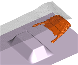
In this section we investigate the propagation of a solitary wave over a submerged breakwater. This test case does not provide a model benchmarking but it is conceived to give a proof of concept of possible applications to typical 3-D problems with wave–structure interactions.
The numerical domain is  $(x,y) \in [0, 24\ \textrm {m} ]\times [0, 16\ \textrm {m}]$, and the submerged breakwater is represented by
 $h(x,y) = [1 - 0.8\,b_1(x)\,b_2(y) ]$, where
 $$\begin{gather} b_1(x) = \left\{ \begin{array}{@{}ll} 1 & \textrm{if } | x - x_0 | \leq L_x/2, \\ - \dfrac{| x - x_0 |}{L_b} + \dfrac{L_x}{2 \, L_b} + 1 & \textrm{if } L_x/2 < | x - x_0 | \leq L_x/2 + L_b, \\ 0 & \textrm{elsewhere}, \end{array} \right. \end{gather}$$
 $$\begin{gather}b_2(y) = \left\{ \begin{array}{@{}ll} 1 & \textrm{if } | y - y_0 | \leq L_y/2, \\ - \dfrac{| y - y_0 |}{L_b} + \dfrac{L_y}{2 \, L_b} + 1 & \textrm{if } L_y/2 < | y - y_0 | \leq L_y/2 + L_b, \\ 0 & \textrm{elsewhere}, \end{array} \right. \end{gather}$$
with  $L_x = 3$ m,
 $L_y = 7$ m,
 $L_b = 2 \sqrt {0.8}$ m and
 $(x_0, y_0) = (12\ \textrm {m}, 8\ \textrm {m})$. The submerged breakwater extends from
 $z = -1$ m (flat seabed) to
 $z=-0.2$ m (top of the breakwater) with a maximum slope
 $s = \sqrt {0.8} / 2 = 0.4472$. A sketch of the breakwater is displayed in figure 19. A uniform Cartesian grid with
 $\Delta x = \Delta y = 0.1$ m is used in the horizontal plane, while a stretched mesh is used in the vertical direction, with
 $\Delta z = 0.05$ m for
 $z \geq -0.25$ m, increasing to
 $3 \Delta z$ at
 $z=-1.15$ m.
Pulse-like wave on a submerged breakwater. Sketch of the bathymetry and isocontours of the bottom, i.e.  $z = - h(x,y)$.

A solitary wave with  $\epsilon = 0.3$ (see Fenton Reference Fenton1972) enters the domain from the boundary at
 $x=0$, while an open boundary is set opposite (i.e. at
 $x=24$ m), and two walls with free-slip conditions are placed at
 $y=0$ and
 $16$ m. The input wave signal is set so that at
 $t=0$, the wave height at the inflow boundary is
 $10^{-5}$ m. Wave breaking starts at
 $t = 7.80\ \textrm {s}$ along the rear edge at the top lee side of the breakwater, namely at about
 $x = 13.55$ m for
 $y \in [5.5\ \textrm {m}, 10.5\ \textrm {m}]$. The maximum wave elevation
 $\eta$ at this location is approximately
 $0.34$ m.
Figure 20 displays a snapshot of the evolution at  $t = 8.51$ s just after the beginning of the wave-breaking event. In particular, figures 20(a,c,e) show the isocontours of the vorticity components, namely
 $| \omega _1 | = 1 \ \textrm {s}^{-1}$,
 $| \omega _2 | = 2 \ \textrm {s}^{-1}$ and
 $| \omega _3 | = 0.2 \ \textrm {s}^{-1}$. As expected, the vorticity in the
 $y$-direction contains the larger amount of energy and generates a well-defined roller just at the lee side of the breakwater (figure 20c). Conversely, the remaining components spread from the rear corners of the submerged structure and are more localized than
 $\omega _2$ (figures 20a,e). Figures 20(b,d, f) display the top views of the vorticity components at the same instant along with the contour and the levels of the wave elevation
 $\eta$ (in the top half of each plot). Maps of the
 $|\omega _3|$ component display patterns of generation similar to those typical of vertical macrovortices induced by finite-length breakers over submerged obstacles (see, for example, Brocchini et al. Reference Brocchini, Kennedy, Soldini and Mancinelli2004; Kennedy et al. Reference Kennedy, Brocchini, Soldini and Gutierrez2006).
Pulse-like wave on a submerged breakwater ( $t=8.51$ s). (a,c,e) Isocontours of the vorticity components (
 $|\omega _1| = 1 \ \textrm {s}^{-1}$,
 $|\omega _2| = 2\ \textrm {s}^{-1}$ and
 $|\omega _3| = 0.2 \ \textrm {s}^{-1}$) along with the free-surface elevation (half-domain). The vertical direction was magnified by a factor
 $3$. (b,d, f) Top view of the same plots with contour of the wave elevation (half-domain).

During the subsequent evolution (see figure 21), the breaking front propagates far from the breakwater and the vorticity generated below it displays a principal roller region ( $\omega _2$ in figures 21c,d) that stays approximately rectilinear, and two lateral tails of vorticity associated with the components
 $\omega _1$ and
 $\omega _3$ (figures 21a,b,e, f). The maps of
 $|\omega _3|$ reveal that the similarity with the evolution of shallow-water macrovortices also characterizes the stages following generation: regions of oppositely signed vorticity get closer to the cross-shore symmetry axis, resembling the pairing of macrovortices that occurs at the lee side of a breakwater (see e.g. figure 3b of Brocchini et al. Reference Brocchini, Kennedy, Soldini and Mancinelli2004).
Pulse-like wave on a submerged breakwater ( $t=10.23$ s). (a,c,e) Isocontours of the vorticity components (
 $|\omega _1| = 1 \ \textrm {s}^{-1}$,
 $|\omega _2| = 2\ \textrm {s}^{-1}$ and
 $|\omega _3| = 0.2\ \textrm {s}^{-1}$) along with the free-surface elevation (half-domain). The vertical direction was magnified by a factor
 $3$. (b,d, f) Top view of the same plots with contour of the wave elevation (half-domain).

A clearer view of such a behaviour is highlighted in figure 22 through the isocontour of modulus of the vorticity, namely  $\| \boldsymbol {\omega } \| = 0.75 \ \textrm {s}^{-1}$. At the initial stages (top panels), the roller forms and increases in magnitude but remains close to the rear edge of the submerged breakwater. Subsequently, the vorticity is transported and stretched by the wave motion as described in the bottom panels. Between
 $t=9.54$ s and
 $t=10.23$ s (bottom panels), the vortical region deforms into a sort of horseshoe vortex whose extremes are essentially made of the components
 $\omega _1$ and
 $\omega _3$. These structures slowly migrate in the wave direction while the principal roller (fed by
 $\omega _2$) undergoes a faster motion below the breaking wave front.
Pulse-like wave on a submerged breakwater. Isocontours of the modulus of the vorticity ( $\| \boldsymbol {\omega } \| = 0.75\ \textrm {s}^{-1}$) along with the free-surface elevation (half-domain) at different times. The vertical direction was magnified by a factor
 $3$.

5. Conclusions
A novel model is proposed for the representation of the wave-breaking dynamics in the context of depth-averaged schemes. This relies on a direct description of the vorticity evolution through a mollified version of the vorticity equation. Such an approach is similar in spirit to that used in the smoothed particle hydrodynamics (SPH) but, differently from that scheme, is implemented within an Eulerian framework. This allows for use of few neighbouring nodes for the discretization of the discrete differential operators, maintaining the same second-order accuracy of the SPH. The reduced number of neighbouring nodes limits the increase of the computational costs, while the representation in the Eulerian framework makes the extension of the model to stretched grids straightforward. Along with the definition of the mollified equations, novel criteria were proposed for the wave-breaking inception and new definitions of the turbulent viscosities, mainly adapting the results of Veeramony & Svendsen (Reference Veeramony and Svendsen2000) to the proposed scheme.
Different experimental data sets available in the literature were used as benchmarks to test the present model in intermediate- and shallow-water conditions. In all cases, this proved to be robust and accurate. Finally, a 3-D problem with a solitary wave interacting with a submerged bar was described to illustrate how the proposed depth-semi-averaged model can well describe intrinsically 3-D flows, characterized by strong vertical accelerations.
The proposed model, blending both pioneering theoretical approaches and consolidated numerical strategies into one robust and accurate tool for simulations of nearshore breaking waves, provides an important alternative to the currently available non-hydrostatic models.
Future works will be devoted to improving some features of the wave-breaking model. In particular, the inclusion of more accurate breaking criteria will be essential to enhance the prediction of the point of the incipient breaking on the wave front. Along with this, a detailed study on the form/structure of the vorticity datum at the free surface will be of fundamental importance to attain a reliable and more precise estimate of the roller region and of the dissipation induced by the vortical structures.
Acknowledgements
The research activity has been developed within the project area ‘Applied Mathematics’ of the Department of Engineering, ICT and Technology for Energy and Transport (DIITET) of the Italian National Research Council (CNR). The authors thank Dr N. Iravani for providing them with the data used in the comparisons of §§ 4.2 and 4.3, and Professors A. Duran and G. Richard for the experimental data of § 4.5.
Funding
This work was partially supported by the FUNBREAK-PRIN2017 project funded by the Italian Ministry MIUR under grant agreement no. 20172B7MY9 $\_$003 and by the ‘NAvi efficienti tramite l'Utilizzo di Soluzioni tecnologiche Innovative e low CArbon’ PNR 2015-2020 MIUR Project, code ARS01
 $\_$00334.
Declaration of interests
The authors report no conflict of interest.
Appendix A. Details of implementation
Here, we summarize the main changes of the present version of the model with respect to those described in Antuono et al. (Reference Antuono, Colicchio, Lugni, Greco and Brocchini2017, Reference Antuono, Valenza, Lugni and Colicchio2019).
We first deal with the rearrangement of the nonlinear term in the momentum equation. The nonlinear term contained in Antuono et al. (Reference Antuono, Colicchio, Lugni, Greco and Brocchini2017, Reference Antuono, Valenza, Lugni and Colicchio2019) is:
 \begin{align} &\boldsymbol{\nabla} \boldsymbol{\cdot} \left[ \int_{{-}h}^{\eta} \, \textrm{d}z \int_{z}^{\eta} ( \boldsymbol{U} + \delta \boldsymbol{u} ) w \,\textrm{d}\zeta \right] -\int_{{-}h}^{\eta} w [ w + h_t + ( \boldsymbol{U} + \delta \boldsymbol{u} ) \boldsymbol{\cdot} \boldsymbol{\nabla} h ] \, \textrm{d}z \nonumber\\ &\quad =I \boldsymbol{\nabla} \boldsymbol{\cdot} \boldsymbol{U} + \boldsymbol{U} \boldsymbol{\cdot} \boldsymbol{\nabla} I - ( U \boldsymbol{\cdot} \boldsymbol{\nabla} h ) \varUpsilon_B + \delta D_{isp} , \end{align}
where  $I$ and
 $\varUpsilon _B$ are defined in § 2, and
 \begin{equation} \delta D_{isp} = \boldsymbol{\nabla} \boldsymbol{\cdot} \left[ \int_{{-}h}^{\eta} \, \textrm{d}z \int_{z}^{\eta} \delta \boldsymbol{u}\,w \,\textrm{d}\zeta \right] - \int_{{-}h}^{\eta} w [ w + h_t + \delta \boldsymbol{u} \boldsymbol{\cdot} \boldsymbol{\nabla} h ] \, \textrm{d}z . \end{equation}
Now using (2.2) and the continuity equation, we write
 \begin{equation} \boldsymbol{\nabla} I = \boldsymbol{M} - \boldsymbol{Q} + \varUpsilon_B\,\boldsymbol{\nabla} h , \quad \boldsymbol{\nabla} \boldsymbol{\cdot} \boldsymbol{U} ={-} \frac{d_t + \boldsymbol{U} \boldsymbol{\cdot} \boldsymbol{\nabla} d}{d} , \end{equation}
and, substituting these inside (A1), we obtain
 \begin{equation} (A1) ={-} \frac{I}{d}\,( h_t + \eta_t+ \boldsymbol{U} \boldsymbol{\cdot} \boldsymbol{\nabla} {d} ) + \boldsymbol{U} \boldsymbol{\cdot} ( \boldsymbol{M} - \boldsymbol{Q} ) + \delta D_{isp} . \end{equation}
The term  $\eta _t$ comes from the contribution proportional to
 $\boldsymbol {\nabla } \boldsymbol {\cdot } \boldsymbol {U}$ in (A1) and is the main source of instability when the wave steepness increases. For this reason, it has to be replaced with an equivalent expression that does not contain time derivatives. In particular, we consider the kinematic free-surface boundary condition, namely
 $\eta _t = w_F - \boldsymbol {U}\boldsymbol {\cdot } \boldsymbol {\nabla } \eta - \delta \boldsymbol {u}_F \boldsymbol {\cdot } \boldsymbol {\nabla } \eta$, and observe that (2.7a,b) evaluated at the free surface lead to
 \begin{equation} \delta \boldsymbol{u}_F ={-} w_F\,\boldsymbol{\nabla} \eta + \frac{\boldsymbol{M}}{d} - \boldsymbol{U} + \boldsymbol{R}_F . \end{equation}
Combining the above expressions, we obtain
 \begin{equation} \eta_t = w_F ( 1 + \| \boldsymbol{\nabla} \eta \|^{2} ) - \left( \frac{\boldsymbol{M}}{d} + \boldsymbol{R}_F \right) \boldsymbol{\cdot} \boldsymbol{\nabla} \eta . \end{equation}
Substituting this formula in (A4), we find
 \begin{equation} (A1) ={-} \frac{I}{d} \left[ h_t + w_F N_F^{2} - \left( \frac{\boldsymbol{M}}{d} + \boldsymbol{R}_F \right) \boldsymbol{\cdot} \boldsymbol{\nabla} \eta + \boldsymbol{U} \boldsymbol{\cdot} \boldsymbol{\nabla} d \right] + \boldsymbol{U} \boldsymbol{\cdot} ( \boldsymbol{M} - \boldsymbol{Q} )+ \delta D_{isp} . \end{equation}
The term  $\boldsymbol {U} \boldsymbol {\cdot } ( \boldsymbol {M} - \boldsymbol {Q} )$ is included in the tensor
 $d (\boldsymbol {U}\otimes \boldsymbol {U})$ described in the previous versions of the model (see Antuono et al. Reference Antuono, Colicchio, Lugni, Greco and Brocchini2017, Reference Antuono, Valenza, Lugni and Colicchio2019) to give the following tensor for the nonlinear momentum flux:
 \begin{align} &\left( \begin{array}{cc} d U_1^{2} & d U_1 U_2 \\ d U_2 U_1 & d U_2^{2} \end{array} \right) + \left( \begin{array}{cc} \boldsymbol{U} \boldsymbol{\cdot} ( \boldsymbol{M} - \boldsymbol{Q} ) & 0 \\ 0 & \boldsymbol{U} \boldsymbol{\cdot} ( \boldsymbol{M} - \boldsymbol{Q} ) \end{array} \right) \nonumber\\ & \quad = \left( \begin{array}{cc} \boldsymbol{U} \boldsymbol{\cdot} \boldsymbol{M} - d U_2^{2} & d U_1 U_2 \\ d U_2 U_1 & \boldsymbol{U} \boldsymbol{\cdot} \boldsymbol{M} - d U_1^{2} \end{array} \right) . \end{align}
The remaining contributions give the term  $D_{isp}$ described in § 2. The derivation of term
 $p_b$ is similar to that of
 $D_{isp}$ and therefore is not reported here.
The advantage of the proposed rearrangement of the nonlinear dispersive terms is illustrated in figure 23 for the benchmark described in § 4.1, using the same spatial discretization. The breaking model is turned off, since in Antuono et al. (Reference Antuono, Colicchio, Lugni, Greco and Brocchini2017, Reference Antuono, Valenza, Lugni and Colicchio2019) this was not available. The formulation used in Antuono et al. (Reference Antuono, Colicchio, Lugni, Greco and Brocchini2017, Reference Antuono, Valenza, Lugni and Colicchio2019) leads to the generation of spurious high-frequency noise in both the free-surface and generalized mass flux signals already at  $t = 1.395\ \textrm {s}$, i.e. before the breaking event occurs (namely, at about
 $t=1.66\ \textrm {s} \unicode{x2013} 1.72\ \textrm {s}$). In fact, such an issue makes the breaking model inapplicable. A study of the influence of the spatial resolution has been done by changing the horizontal discretization. Indicating by
 $\Delta x$ the reference spatial step (see § 4.1), we observe that the spurious oscillations disappear when the discretization is halved (i.e.
 $2\,\Delta x$ is used). On the contrary, the occurrence of spurious oscillations worsens with a finer resolution (namely,
 $\Delta x/2$), confirming the existence of a numerical instability. Conversely, the novel formulation of the nonlinear dispersive terms is stable and convergent, as shown in figure 24. Figure 24(a) displays the global total energy, i.e.
 \begin{equation} \mathscr{E}_T = \frac{1}{2 \mathscr{V}}\int_{D} \left[ g \eta^{2} + d \| \boldsymbol{U} \|^{2}+ \int_{{-}h}^{\eta} ( \delta u^{2} + \delta v^{2} + w^{2} ) \, \textrm{d}z \right] \, {{\rm d}}V , \end{equation}
where  $\mathscr {V}$ is the total volume of water, and
 $D$ indicates the 2-D domain in the
 $(x,y)$-plane. Figure 24(b) shows the global total energy of the depth averaged system, i.e.
 \begin{equation} \bar{\mathscr{E}}_T = \frac{1}{2 \mathscr{V}}\int_{D} [ g \eta^{2} + d \| \boldsymbol{U} \|^{2} ]\, {{\rm d}}V . \end{equation}
Experiments of Lucarelli et al. (Reference Lucarelli, Lugni, Falchi, Felli and Brocchini2019). Comparison between the formulation of the nonlinear dispersive terms given in Antuono et al. (Reference Antuono, Colicchio, Lugni, Greco and Brocchini2017, Reference Antuono, Valenza, Lugni and Colicchio2019) (red lines) and the present one (black lines) at  $t = 1.395~s$. (a) Free surface elevation. (b) Generalized mass flux.

Experiments of Lucarelli et al. (Reference Lucarelli, Lugni, Falchi, Felli and Brocchini2019). Convergence analysis by varying the horizontal discretization:  $\Delta x = 0.01$ (black lines),
 $\Delta x = 0.005$ (red lines) and
 $\Delta x = 0.0025$ (green lines). (a) Time history of the global total energy. (b) Time history of the global total energy of the depth-averaged subsystem.

Concerning the reconstruction of the numerical fluxes, in the present model we still rely on the use of a fourth-order reconstruction as described in Yamamoto & Daiguji (Reference Yamamoto and Daiguji1993), but differently from the previous versions of the scheme, we set the parameters of the reconstruction as  $b_1 = 1$ and
 $b=3$. In Antuono et al. (Reference Antuono, Colicchio, Lugni, Greco and Brocchini2017, Reference Antuono, Valenza, Lugni and Colicchio2019), the former parameter was set equal to 2, but this led to an increase of the energy of the numerical scheme for long-time evolutions (e.g. propagation of Stokes waves over several periods). This phenomenon was observed only for very fine spatial resolutions and led, after several cycles, to the generation of small-amplitude high-frequency spurious noise. On the contrary, the choice
 $b_1=1$ completely removes this issue at the cost of a slightly more dissipative scheme.
Appendix B. The vertical component of the vorticity field
Let us denote by  ${\hat {\boldsymbol {\nabla }}}$ the gradient in three spatial dimensions. Then using the relations listed in § 2, we write
 \begin{equation} \hat{\boldsymbol{\nabla}} \varUpsilon = \left(\frac{M_1}{d} + R_1 - u, \frac{M_2}{d} + R_2 - v, -w \right). \end{equation}
By construction, the following relation has to hold true:
 \begin{align} 0 = \hat{\boldsymbol{\nabla}} \times \hat{\boldsymbol{\nabla}} \varUpsilon &= ( - R_{2,z} - \omega_1 )\,\boldsymbol{\hat{e}_1} + ( R_{1,z} - \omega_2 )\,\boldsymbol{\hat{e}_2}\nonumber\\ & \quad + \left[\left( \frac{M_2}{d} + R_2 \right)_x - \left( \frac{M_1}{d} + R_1 \right)_y - \omega_3 \right] \boldsymbol{\hat{e}_3} , \end{align}
where  $\boldsymbol {\hat {e}_1}, \boldsymbol {\hat {e}_2}, \boldsymbol {\hat {e}_3}$ are the unit vectors in the Cartesian directions. By definition,
 $R_{1,z} = \omega _2$ and
 $R_{2,z} = -\omega _1$, and consequently, the horizontal components are identically null. Conversely, the third component gives the expression of
 $\omega _3$ as a function of
 $\boldsymbol {M}/d$ and
 $\boldsymbol {R}$. Using the 2-D gradient, we rearrange it in the format
 \begin{equation} \omega_3 = \boldsymbol{\nabla} \times \left(\frac{\boldsymbol{M}}{d} + \boldsymbol{R} \right). \end{equation}
Incidentally, we observe that this expression implies  $\hat {\boldsymbol {\nabla }} \boldsymbol {\cdot } \boldsymbol {\omega } = 0$, confirming that the vorticity field represented theoretically by the proposed model is solenoidal.
Appendix C. Smoothed operators over non-uniform grids
Let us consider a non-uniform Cartesian grid with steps  $\Delta x_m$ in the coordinate directions. The weight function
 $W$ is adapted to such a grid as follows:
 \begin{equation} W ( \boldsymbol{y} -\boldsymbol{x} ) = W( \sigma ), \quad \textrm{where } \sigma^{2} = \sum_{m=1}^{3} \frac{(y - x)_m^{2}}{a_m^{2}}, \end{equation}
with  $a_m = \beta \,\Delta x_m$, and
 $\beta$ a dimensionless stretching parameter. Consequently, the
 $m$th component of the gradient of
 $W$ is given by
 \begin{equation} [ \hat{\boldsymbol{\nabla}}_x W(\sigma )]_m ={-} \frac{(y-x)_m}{a_m^{2}}\, \frac{1}{\sigma}\,\frac{\textrm{d} W}{\textrm{d} \sigma} . \end{equation}
Incidentally, we highlight that the above expression still satisfies the anti-symmetry relation  $\hat {\boldsymbol {\nabla }}_y W( \boldsymbol {x} - \boldsymbol {y} ) = - \hat {\boldsymbol {\nabla }}_x W( \boldsymbol {x} - \boldsymbol {y} )$ that has been used extensively to derive the model in § 3.
In this work, we use the C2-Wendland kernel in three spatial dimensions described in Wendland (Reference Wendland1995). Over a unitary sphere (i.e.  $a_m =1$ for
 $m=1,2,3$), this reads
 \begin{equation} W(\sigma) = \left\{
\begin{array}{@{}ll} C_W (4 \sigma + 1 ) ( 1 - \sigma )^{4} &
\textrm{for } \sigma \leq 1,\\[2pt] 0 & \textrm{elsewhere},
\end{array} \right. \end{equation}
wherein  $C_W = 21/(2 {\rm \pi})$, and finally
 \begin{equation}
\frac{1}{\sigma}\,\frac{\textrm{d} W}{\textrm{d} \sigma} =
\left\{ \begin{array}{@{}ll} - 20 C_W ( 1 - \sigma )^{3} &
\textrm{for } \sigma \leq 1,\\[2pt] 0 & \textrm{elsewhere}.
\end{array} \right. \end{equation}
In the present model, the domain of the weight function  $W$ is set equal to an ellipsoid with semi-axes equal to
 $a_m = 1.8\,\Delta x_m$ (i.e.
 $\beta = 1.8$). In this case,
 $\sigma$ is given by the expression in (C1), and
 $C_W = 21/(2 {\rm \pi}a_1 a_2 a_3)$.
Finally, we observe that in two dimensions, the expression of the Wendland kernel is the same as described in (C3), but the re-normalization constant has to be modified in  $C_W = 7/{\rm \pi}$. Accordingly, for a stretched grid, we obtain
 $C_W = 7/({\rm \pi} a_1 a_2)$.
Appendix D. Details on the reconstruction of the inflow data
Here, we summarize briefly the procedure used in the test case of § 4.5 to obtain the inflow input data  $M_1$ and
 $\varUpsilon _x$ from knowledge of
 $\eta$. The main hypotheses at the basis of our procedure are that the waves are small (i.e. the linear approximation can be used), that the propagation occurs in shallow-water conditions, and finally, that the waves are purely entering the domain (i.e. no reflection).
In one spatial dimension, the linearized governing equations and the linearized free-surface condition read
 \begin{equation} \frac{\partial \eta}{\partial t} ={-} h U_x , \quad \frac{\partial}{\partial t} \left( \frac{M_1}{d} \right) ={-} g \eta_x , \quad w_F = \frac{\partial \eta}{\partial t} . \end{equation}
Under shallow-water conditions, a linear profile is assumed for the vertical velocity, namely
 \begin{equation} w = w_F \left[ 1 - \left(\frac{\eta-z}{d} \right) \right] \Rightarrow \varUpsilon = \int_{z}^{\eta} w \,\textrm{d}\zeta = w_F \left[ (\eta -z) - \frac{( \eta-z)^{2}}{2 d} \right] . \end{equation}
Neglecting the nonlinear contributions, we obtain
 \begin{equation} \varUpsilon_x = ( w_F )_x \left[ (\eta -z) - \frac{( \eta-z)^{2}}{2 d} \right] , \end{equation}
and, using the definition of  $M_1$, we find
 \begin{equation} \frac{M_1}{d} = U + \frac{1}{d} \int_{{-}h}^{\eta} \varUpsilon_x \, \textrm{d}z = U + ( w_F )_x\,\frac{d^{2}}{3} . \end{equation}
The spatial derivative of the vertical velocity component can be expressed as a function of  $(M_1/d)$ by using relations (D1a–c). This leads to
 \begin{equation} ( w_F )_x ={-} \frac{1}{g}\,\frac{\partial^{2}}{\partial t^{2}} \left( \frac{M_1}{d} \right). \end{equation}
Since at the leading order  $(M_1/d) = u_F$ (see Antuono et al. Reference Antuono, Valenza, Lugni and Colicchio2019), the following equation linking
 $U$ and
 $u_F$ is achieved:
 \begin{equation} \frac{d}{3 g}\,\frac{\partial^{2} u_F}{\partial t^{2}} + u_F = U . \end{equation}
In shallow-water conditions, it is  $u_F \simeq U$ and the above expression can be rearranged as
 \begin{equation} u_F = U - \frac{d}{3 g}\,\frac{\partial^{2} U}{\partial t^{2}} . \end{equation}
The final step is to assume that the wave is purely entering the domain. As shown in Antuono (Reference Antuono2010) and Antuono & Brocchini (Reference Antuono and Brocchini2010), for the case described in § 4.5, this corresponds to the approximation
 \begin{equation} U = \sqrt{\frac{d}{g}}\,\eta , \end{equation}
which gives the depth-averaged velocity  $U$ as a function of
 $\eta$. Substitution of the above expression inside (D7) allows one to compute
 $u_F = M_1/d$, and consequently
 $M_1$. Finally, using (D5) and (D3), we obtain the expression for
 $\varUpsilon _x$ as a function of
 $\eta$.


 Open access

