2. LITERATURE REVIEW

Warranty theory has been heavily studied over the past two decades. Blischke and Murthy [3] wrote a comprehensive reference for the subject. They discussed many different types of warranty policy, including many warranty policies currently implemented in industry. Numerous cost and optimization models were developed from both the consumer's and the manufacturer's point of view, including life cycle and long-run average cost models. We use these models to compute the expected warranty cost of a product in our numerical examples.

Many of the early papers on warranty theory discussed the costs and other effects that are associated with warranties. Glickman and Berger [7] considered the effect of warranty on demand by assuming that demand increases as the warranty period increases.

Warranty costs affect both the buyer and the seller. Mamer [12] wrote the first paper to provide a comprehensive model of both the buyer's and seller's expected costs and long-run average costs for the free-replacement warranty. Our research focuses on the manufacturers' view of warranty costs.

The concept of a warranty reserve is a topic of many research works. The initial papers on warranty reserves discussed here considered a fixed product lot size throughout the life cycle of a product (or, equivalently, a fixed cumulative failure rate). Menke [14] wrote one of the first papers to address the warranty reserve problem. He concentrated on calculating the expected warranty cost over a given warranty period for two types of pro-rata warranty policy (linear rebate and lump-sum rebate) assuming a constant product failure rate. Amato and Anderson [1] extend Menke's model by allowing the reserve fund to accrue interest, requiring the consideration of discounted costs. A comparison to Menke's results is made, concluding that discounting significantly reduces the expected warranty reserve over longer periods of time. Both models are rather limited in scope because they only consider pro-rata warranty policies and an exponential failure distribution.

Balcer and Sahin [2] derived the moments of the total replacement cost for both the free-replacement and pro-rata warranty policies during the product life cycle. They assumed that successive failure times form a renewal process.

Mamer [13] used renewal theory to model repeated product failures over the life cycle of the product. He incorporated discounting in his model and allowed for a general failure distribution.

Tapiero and Posner [18] allowed for a portion of each sale to be set aside for future warranty costs. The contributions to the reserve fund and the items sold occur at a constant rate. The claims were generated according to a compound Poisson process and they used a sample path technique to compute the long-run probability distribution of the warranty reserve.

Eliashberg, Singpurwalla, and Wilson [6] calculated the reserve for a product whose failure rate is indexed by two scales: time and usage. They allowed for a general failure rate and assumed a form of imperfect repair. The warranty reserve was computed to minimize a loss function for the manufacturer.

Ja, Kulkarni, Mitra, and Patankar [9] computed the distribution of the total discounted warranty cost over the life cycle of the product. They analyzed the discounted warranty cost of a single sale under many different policies and then considered different stochastic sales processes. A single contribution to the reserve is made at the beginning of the life cycle. However, the subtractions from the reserve due to warranty costs are tracked as a function of time.

Another application related to the warranty reserve problem is the insurance premium problem. An insurance company must decide on the monthly premium to charge a certain class of customer. Low premiums result in loss to the insurer, whereas high premiums result in loss of business to the competition. A discussion of this can be found in [16]. There are other related problems, including the funding of a company's pension plan. Many of these problems are solved using actuarial models, particularly collective risk (loss) models (see [4,11] for references on this subject). However, the current models do not incorporate the number of policies insured by the company at any given time.

The above-described works illustrate many different models for computing the warranty reserve. However, they assume that the reserve is either funded at the beginning of the product sales period or at a constant rate. We extend this research by modeling contributions to the reserve after each sale and allowing the cumulative warranty claim rate to depend on the sales process.

3. PROBLEM FORMULATION

We begin by introducing some notation and assumptions. Let S(t) be the total number of sales during (0,t]. We assume that {S(t),t ≥ 0} is a nonhomogeneous Poisson process with a known rate function (sales rate) θ(·); we call this an NPP(θ(·)). Let S_j denote the time of the jth sale. Each item is under warranty for a random amount of time. The warranty durations are independent and identically distributed (i.i.d.) with common cumulative distribution function (c.d.f.) F(·) and mean w. Also, the warranty durations are independent of any future failures. Note that this allows for a constant warranty period. Let X(t) denote the number of items under warranty at time t. Thus, {X(t),t ≥ 0} is the number in an M/G/∞ queue with an NPP arrival process and i.i.d generally distributed service times.

We assume that the customer always makes a warranty claim at each product failure. The repairs are instantaneous and the times between repairs (on a given item) are i.i.d. exp(λ). Thus, the rate at which failures occur at time t is given by λX(t). The repair cost of the ith failure (at time Y_i) is D_i, a random variable. The D_i's are i.i.d. and are independent of the failure time.

The manufacturer maintains a reserve account to take care of the warranty claims arising during the planning period of length T. The reserve account starts with an initial level R₀, and at each sale, an amount c is contributed to the account. Let R(t) be the amount in the reserve at time t, where t = 0 represents the beginning of the planning period. The reserve fund accrues interest at constant rate α > 0. Thus, we have

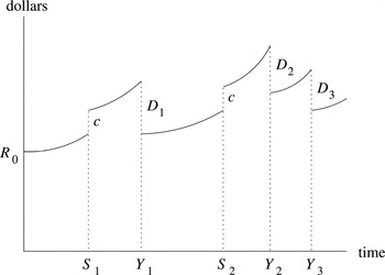
Figure 1 shows a typical sample path of the warranty reserve over time.

Example of a warranty reserve account.

The manufacturer must decide on the initial reserve level, R₀, and the contribution amount to the reserve from each sale, c, at the beginning of the planning period. We assume that the manufacturer is guided by two principles in this:

1. Ensure that the warranty reserve at the end of the planning period stays positive with a prespecified probability β; that is,
   
2. Satisfy all of the expected total warranty costs in (0,t] by the expected total contributions made in (0,t]. Thus, since the reserve fund starts with R₀, it should grow to R₀ e^αT in expectation by time T. In other words,
   

It is clear that we need to compute the distribution of R(T) in order to use Eq. (2). However, computing the distribution is highly intractable, and we will approximate it by a Normal distribution using the first and second moments of R(T). It is also clear that the number of items under warranty at time 0 and their remaining warranty periods will influence the distribution of R(T). Hence, we turn our attention to the problem of analyzing these quantities in the next two sections.

4. PROBABILITY DISTRIBUTION OF THE NUMBER OF ITEMS UNDER WARRANTY

Let X₁(t) represent the number of items under warranty at time t that were sold after time 0, and let X₂(t) represent the number of items under warranty at time t that were sold prior to time 0. Thus, the total number of items under warranty is given by

In this section we derive the distributions for X₁(t) and X₂(t).

4.1. Distribution of X₁(t)

Recall that θ(·) is the sales rate and F(·) is the warranty length distribution. Since there is no bound to the number of items under warranty, it is clear that the {X₁(t),t ≥ 0} process is the number in the M_t /G/∞ queue with arrival rate θ(·) and service time distribution F(·), starting with X₁(0) = 0.

The following result was established independently by Palm [15] and Khintchine [10]. Most recently, Eick, Massey, and Whitt [5] provided a simpler proof of this result and developed some further results for the M_t /G/∞ queue.

Theorem 1: Let Z(t) be the number of customers in an M_t /G/∞ queue at time t with arrival rate θ(·) and i.i.d. service times with common c.d.f. F(·). Assume Z(0) = 0. Then, for each time point t ≥ 0, Z(t) is a Poisson random variable with mean

Using the above theorem and the earlier observation, we see that the moments of X₁(t) are given by

4.2. Distribution of X₂ (t)

We consider two possible cases for the items sold prior to time 0: (1) the manufacturer fully knows the remaining warranty durations of all items under warranty at time 0 or (2) the remaining warranty durations are i.i.d. random variables with common c.d.f. Q(·). Case (1) is easy; the entire sample path of X₂(t) is a deterministic function. In case (2) the probability that the remaining warranty duration of an item is greater than t, given that it was under warranty at time 0, is 1 − Q(t). Hence,

where X(0) is the number of items under warranty at time 0. The moments are

One choice for Q(t) is obtained from the stationary distribution of the remaining service times in an M_t /G/∞ queue in steady state. For the special case of a homogeneous Poisson arrival process, we use the following theorem from Takács [17].

Theorem 2 (Takács [17, Thm.3.2.2]): Let Z(t) be the number of customers at time t in an M/G/∞ queue with arrival rate θ, service time distribution F, and mean service time τ < ∞. Then, in steady state, the remaining service times of all customers in the system are i.i.d. random variables with common distribution

Therefore, under the assumption of the Poisson sales process, we have that the remaining warranty periods are i.i.d. random variables with common distribution

This result can be extended to the case of a nonhomogeneous Poisson process, as shown in the following theorem.

Theorem 3: Let Z(t) be the number of customers at time t in an M_t /G/∞ queue with arrival rate function θ(·), service time distribution F, and mean service time τ < ∞. Suppose that the arrival process begins at time −∞. Then the remaining service times of the customers in the system at time t are i.i.d. random variables with common c.d.f. F_e(t,x) given by

The proof is given in the Appendix.

By setting t = 0, we can use the following for Q(x):

It is easy to check that Eq. (9) reduces to Eq. (8) if θ(t) = θ for all values of t.

Since X₁(t) and X₂(t) are independent of each other, we compute the moments of X(t) as

In the next section we will use the moments of X(t),X₁(t), and X₂(t) in the computation of the moments of R(t).

5. DIFFERENTIAL EQUATIONS FOR MOMENTS OF R(t)

In this section we compute

We first write

where R₁(t) is the portion of the reserve related to the new items X₁(t), and R₂(t) is the portion of the reserve related to the old items X₂(t). Thus, in R₁(t), we add contributions from new purchases and only subtract the claims generated by new items. In R₂(t), there are no new contributions, so we only subtract claims generated by old items. The two processes {R₁(t),t ≥ 0} and {R₂(t),t ≥ 0} are independent. Hence, if we compute

we can compute the moments of R(t) as follows:

There are two cases for the state at the beginning of the sales period: (1) the remaining warranty periods are known at time 0 and (2) the remaining warranty periods are unknown at time 0, with the distribution discussed in Section 4.2. We cover the second case here and leave the first case as an easy extension.

We will use Δ_h to indicate the change in a function from t to t + h. For example, Δ_h R(t) = R(t + h) − R(t). Finally, we will use the standard o(h) notation for a function g(h) when

Recall that S(t) is the total sales during (0,t]. Also, let D(t) be the total undiscounted cost of all claims up to time t. In the results that follow, we will need expressions for E [Δ_h S(t)] and E [Δ_h D(t)], where h is small. Since {S(t),t ≥ 0} is an NPP(θ(·)), we know that for sufficiently smooth θ(·),

Next we compute E [Δ_h D(t)]. Let N(t) represent the number of claims from time 0 to t. For a given sample path of {X(t),t ≥ 0}, {N(t),t ≥ 0} is an NPP(λX(·)). We have

where {D_i,i ≥ 1} are i.i.d. with common mean E [D] and second moment E [D²] and are independent of {N(t),t ≥ 0}. Therefore,

Similarly,

We next introduce notation for item failure rates. Consider an arbitrary item that was sold in [0,t]. Let U be its time of sale. Then U has c.d.f.

where

Let W represent the warranty period random variable. Then the probability that the item is under warranty at time t is P(U + W > t). Given that it is under warranty at time t, the probability that its warranty expires in [t,t + δ] is given by

Since the warranty periods are i.i.d. and the sales process is an NPP, we see that the items are independent of each other. Hence, if X₁(t) = i, the probability that a single items fails in [t,t + δ] is ih₁(t)δ + o(δ). We do a similar analysis for the items under warranty at time 0. We assume that the remaining lifetimes are unknown but are independent of each other. The probability that an item is still under warranty at time t is 1 − Q(t), and the probability that its warranty expires in [t,t + δ] is given by h₂(t)δ, where

For convenience, we define

We are now ready to compute the moments of R(t).

Theorem 4: Let r(t) = E [R(t)]. Then

with initial condition r(0) = R₀.

Proof: We look at the change in the reserve from time t to time t + h, where h is small. We have

Taking expectation on both sides, we get

Diving by h and taking the limit as h → 0 yields Eq. (15). █

To derive the differential equation for the second moment, we first give a lemma.

Lemma 1: Let r₁(t) = E [R₁(t)], v(t) = E [R₂(t)X₂(t)], and u(t) = E [R(t)X(t)]. Then

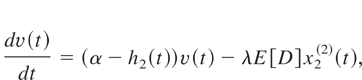
with initial conditions r₁(0) = 0, v(0) = X(0)R₀, and u(0) = X(0)R₀. Also, x₁(t) satisfies Eq. (4), x₂(t) satisfies Eq. (6), x₂⁽²⁾(t) satisfies Eq. (7), x⁽²⁾(t) satisfies Eq. (11), h₁(t) satisfies Eq. (12), and h₂(t) satisfies Eq. (13).

Proof: We apply the same techniques as in the proof of Theorem 4. We omit the details for the sake of brevity. █

Using the lemma, we can now provide the differential equation for the second moment of R(t) in the following theorem.

Theorem 5: Let r⁽²⁾(t) = E [R²(t)] and r(t),u(t),v(t), and r₁(t) be defined as earlier. Then

where r⁽²⁾(0) = R₀².

Proof: We proceed as follows. First, we look at the expression R(t + h) − R(t) for small values of h, where

By squaring both sides of the above expression, rearranging terms, and taking the expectation of both sides, we obtain six expressions on the right-hand side. Each of the terms can be directly computed to obtain the result. █

Equations (15)–(19) form a triangular system of equations for the first and second moments of R(t) that can be solved recursively. We can also use a software package, such as MATLAB, to solve the system numerically. Also, we can solve the system analytically by using a software package such as Maple, which is used for the example in the next section. The variance is given by

In the next section we present the general solution to this system and some examples for simple warranty distributions.

6. SOLUTION FOR MOMENTS OF R(t)

We now provide the solution to the differential equations derived in Section 5. For a complete solution, it is necessary to know the functions x(t), x₂(t), x₁(t), x₂(t), h₂(t), h₁(t), H₂(t), and H₁(t). These expressions, defined in Eqs. (4)–(14) of Section 4, depend only on the warranty distribution F(·) and the sales rate θ(·).

Theorem 6: Let r(t), r₁(t), v(t), u(t), and r⁽²⁾(t) be defined as in Section 5. Then we have

Proof: We apply the standard techniques to solve linear differential equations in a backward recursive fashion for each of r(t), r₁(t), v(t), u(t), and r⁽²⁾(t). For the sake of brevity, we omit the details. █

Example: Constant Warranty Period and Constant Sales Rate: We provide the solution for the first and second moments of R(t) for the example of a constant warranty period w and a constant sales rate function θ(t) = θ for all t ≥ 0. The second moment r⁽²⁾(t) is quite complex, so we, instead, provide the variance of R(t).

First, we provide the moments of X₁(t) and X₂(t) and the expressions for F(t), h₁(t), and h₂(t). We assume that the remaining warranty periods of the items sold prior to time 0 is unknown. We apply the result from Section 4.2 to determine the distribution of X₁(t). We have

Applying the formulas for the first and second moments of X₁(t) and X₂(t) yields

Using the expressions for h₁(t) and h₂(t) defined in (12) and (13), we obtain

We consider two cases.

Case 1: 0 ≤ t ≤ w. Here we obtain

where

Case 2: t > w. In this case there are no longer any old items under warranty. We obtain the following:

where

7. DECIDING THE VALUES OF c AND R₀

The manufacturer must decide on the values of c and R₀ at the beginning of a new period, with the goal of satisfying Eqs. (2) and (3). The next theorem gives the main result.

Theorem 7: Equation (3) is satisfied if

As the number of sales goes to infinity, R(T) converges in distribution to a Normal random variable with mean r(T) and second moment r⁽²⁾(T) given in Theorem 6. In this asymptotic regime the inequality (2) is satisfied if

where z_β is the 100βth percentile of a standard Normal distribution.

Proof: From Eq. (20), we see that Eq. (3) is equivalent to solving

This equation does not contain R₀. Eq. (23) yields Eq. (21).

Since the sales process is nonhomogeneous Poisson, the asymptotic normality of R(T) as the sales volume goes to infinity follows a straightforward extension of the result given by Ja [8], which is based on [9]. Therefore, in this asymptotic regime, R(T) is Normally distributed with mean r(T) and the second moment r⁽²⁾(T) given in Theorem 6. Equation (22) follows from this. █

8. NUMERICAL COMPUTATIONS

In this section we present a numerical example. Consider a nonrenewable, free-replacement warranty with constant period 1 year. All of the items are independent and identical, with mean 0.1 failures per year and each replacement cost to the manufacturer is fixed at $100. The sales process is a Poisson process with mean 1000 items/year. We use a continuous discount rate of α = 0.06, implying an annual interest rate on the account of 6.18%. Some products that might have this structure are electronic devices (such as calculators) or small appliances (such as toasters or microwaves). More complex products, such as computers, have similar properties where repairs are “good as new.”

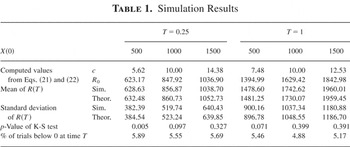
We use Eq. (21) to determine c and we use β = 0.95 (and z_β = 1.645) in Eq. (22) at equality to determine R₀. The results are shown in Table 1 for different values of T, the planning period, and X(0), the initial number of items under warranty. We assume that the remaining warranty periods of these items are unknown. Using Eq. (8), we assume that the remaining warranty periods are uniformly distributed over (0,1) years. Note that in steady state the number of items under warranty is θw = 1000. We simulate 10,000 replications with the above parameters to check for normality of R(t). The p-values from the Kolmogorov–Smirnov (K-S) test for normality are given in Table 1. It is clear that in this example the normal approximation is a better fit for T = 1 than for T = 0.25, since there are more sales in a 1-year period than a 3-month period. As expected, the simulated mean and standard deviation at each time point match up with the theoretical mean and variance.

Simulation Results

We compare the values of c obtained through the heuristic with the expected single-item warranty cost. Let E [C_W(α)] be the expected total warranty cost discounted to present value for a single item. One option for the manufacturer is to contribute this amount to the reserve after each sale. We compute E [C_W(α)] by the following formula (see [3, Sect.4.2]):

where M(·) is the ordinary renewal function associated with the product failure distribution (here M(t) = λt). Substituting the numbers of the example yields E [C_W(α)] = 9.71.

This shows that letting c ≈ E [C_W(α)] is very effective if X(0) ≈ θw. However, if X(0) and θw are far apart, the recommended values of c can be substantially different. Note that for T = 1, the values of c were closer to the expected warranty cost than for T = 0.25.