


1. Introduction
Provided the value of the Reynolds number  $Re$ is not too low, a typical wall-bounded turbulent flow features both large-scale structures located away from but extending down to the wall, and smaller-scale structures which dominate the near-wall region but populate the whole flow. In recent years, the top-down influence of large-scale structures has been thoroughly studied, and considerable efforts have been devoted to their statistical characterization and to the understanding of the anomalous viscous scaling for the near-wall statistics attributed to the outer structures (e.g. Smits, McKeon & Marusic Reference Smits, McKeon and Marusic2011). On the other hand, how the smaller-scale structures residing near the wall affect the large-scale structures away from the wall is less clear.
Early studies addressing such a bottom-up interaction attributed the existence of large-scale motions to agglomeration of smaller-scale events (Guala, Hommema & Adrian Reference Guala, Hommema and Adrian2006), while Toh & Itano (Reference Toh and Itano2005) introduced the idea of a co-supporting cycle where the large structures are directly forced by the near-wall ones. There are also suggestions (Flores, Jiménez & Del Álamo Reference Flores, Jiménez and Del Álamo2007; Hwang & Cossu Reference Hwang and Cossu2010) that large-scale motions in the outer layer can self-sustain and are nearly independent of the buffer layer. Such multi-scale interactions have come into focus only recently, one of the reasons being that they become visible once the Reynolds number of the flow is large, owing to the required separation of scales. Moreover, they have been mostly studied in turbulent channel flow, because of its geometrical simplicity. The tool of choice for such studies is often the spectral analysis of the transport equation for the components of the Reynolds stress tensor (Mizuno Reference Mizuno2016; Lee & Moser Reference Lee and Moser2019). A notable result is that in wall flows the (statistically dominant) energy transfer towards small scales is accompanied by an inverse transfer from small to large scales. However, spectral analysis can only observe energy fluxes in the space of scales, and the concept of scale is limited to homogeneous directions. An alternative tool, the generalized Kolmogorov equation (GKE), seems well suited for this analysis. The GKE was derived by Hill (Reference Hill2001) as an exact budget equation for the second-order structure function: a separation in the inhomogeneous wall-normal direction can be defined, and a description of energy production, dissipation and energy fluxes in the compound space of scales and positions becomes possible.
The GKE has been used, in more or less simplified forms, to describe the effects of inhomogeneity on small-scale turbulence, most often for plane channel flow, although, for example, Mollicone et al. (Reference Mollicone, Battista, Gualtieri and Casciola2018) used the GKE to identify the coherent vortical structures in a separated turbulent flow behind a bump, Togni, Cimarelli & De Angelis (Reference Togni, Cimarelli and De Angelis2015) to describe Rayleigh–Bénard convection, Portela, Papadakis & Vassilicos (Reference Portela, Papadakis and Vassilicos2017) to address the turbulent cascades in the near wake of a square cylinder and Cimarelli et al. (Reference Cimarelli, Mollicone, van Reeuwijk and De Angelis2021) to investigate the entrainment and mixing processes in a turbulent planar temporal jet. Cimarelli, De Angelis & Casciola (Reference Cimarelli, De Angelis and Casciola2013) applied the GKE to a turbulent channel flow and observed that energy fluxes originating in the near-wall region transfer energy backwards towards longer and wider turbulent structures as the distance from the wall increases, and then interact with smaller structures before eventually dissipating. In a further study, Cimarelli et al. (Reference Cimarelli, De Angelis, Jimenez and Casciola2016) identified an additional energy source, which appears in the overlap layer as  $Re$ increases and leads to a complex spatial redistribution of energy which links small dissipative and large energy-containing scales through a mixed cascade. An inverse energy transfer from small- to large-scale motions has been also observed near the wall by Cho, Hwang & Choi (Reference Cho, Hwang and Choi2018) by means of the spectral turbulent kinetic energy balance equation. They provided evidence that the large-scale motions near the wall scale in inner units, and Cheng et al. (Reference Cheng, Li, Lozano-Durán and Liu2020) revealed that the footprints of the large-scale motions manifest as large-scale regions of negative wall friction.
Less attention has been devoted to plane turbulent Couette flow, where to our knowledge a GKE analysis has never been attempted. However, Couette flow is as geometrically simple as Poiseuille flow, and represents an interesting alternative for probing the inner/outer interactions at direct numerical simulation (DNS)-accessible Reynolds numbers. In fact, this is one of the most fundamental configurations of wall-bounded turbulence, where two indefinite parallel plates move at constant relative velocity and produce a purely shear-driven turbulence.
A key difference with pressure-driven Poiseuille flow is that the mean velocity gradient for Couette flow does not vanish at the centreline, leading to a non-zero production of turbulent kinetic energy in the core region. Moreover, already at relatively low  $Re$, Couette flow contains large-scale motions in the form of elongated streamwise vortices filling the space between the two walls: for example, Tsukahara, Kawamura & Shingai (Reference Tsukahara, Kawamura and Shingai2006) found evidence of these vortices already at
 $Re_\tau =52$ and Lee & Moser (Reference Lee and Moser2018) described them at
 $Re_\tau =93$. These structures, traced down by Illingworth (Reference Illingworth2020) to the linearized Squire and Orr–Sommerfeld operators, can be identified in both flows, but Couette flow creates stronger structures out of the mean shear (Andreolli, Quadrio & Gatti Reference Andreolli, Quadrio and Gatti2021). The mutual interaction between the large streamwise-elongated rolls and the smaller eddies in turbulent flow is not entirely understood. Lee & Moser (Reference Lee and Moser2019) discussing high-
 $Re$ Poiseuille flow observed how energy is transferred more or less isotropically from the largest structures down to the dissipation scales via nonlinear interactions. However, Kawata & Tsukahara (Reference Kawata and Tsukahara2021) artificially constrained the wall-parallel dimensions of the computational domain for a Couette flow to indirectly characterize direct and inverse cascades, and used data computed from spanwise-minimal domains to suggest that the interscale energy transfers observed by Lee & Moser (Reference Lee and Moser2019) with one-dimensional spanwise spectral analysis might pertain to the inner and outer dynamics, without actually representing their interactions. Kawata & Alfredsson (Reference Kawata and Alfredsson2018) experimentally studied Couette flow via stereoscopic particle image velocimetry, and were first to consider the Reynolds shear stress. They observed an inverse cascade from the small scales near the wall to the large scales away from the wall, but only for the shear stress. The inverse cascade mainly affects the near-wall region, and exerts a bottom-up influence from the near-wall region to the channel core. In their experimental study, Kawata & Alfredsson (Reference Kawata and Alfredsson2018) had access to the three velocity components in nine wall-parallel planes (outside the near-wall region), and had to resort to the continuity equation to indirectly assess the wall-normal derivative of the wall-normal velocity component, whereas the remaining wall-normal derivatives were not considered in the transfer. Moreover, in their analysis the streamwise separation was neglected.
The present work comprehensively addresses the interscale exchanges across the wall-normal direction in a turbulent plane Couette flow, and builds upon a recent extension of the GKE (Gatti et al. Reference Gatti, Chiarini, Cimarelli and Quadrio2020) that enables the observation of each component of the Reynolds stress tensor in the compound space of scales and wall distances. This extended tool, the anisotropic generalized Kolmogorov equations or AGKE, will be used here to study a Couette flow computed with DNS at  $Re_\tau \approx 100$, the highest
 $Re$ considered by Kawata & Alfredsson (Reference Kawata and Alfredsson2018). Our aim is to address the mechanisms of direct/inverse cascading, and to identify bottom-up and top-down processes. The paper is organized as follows. First, in § 2 the budget equations for the structure function tensor are recalled, and the simulation which produced the DNS database used later for statistical analysis is briefly described. Then, in § 3 the main results concerning the components of the Reynolds stresses tensor are presented, and in § 4 a concluding discussion is given.
2. Methods
This work relies upon the AGKE budget equations as introduced by Gatti et al. (Reference Gatti, Chiarini, Cimarelli and Quadrio2020) to tackle the inhomogeneity and the anisotropy of a generic turbulent flow. These equations are briefly recalled here for completeness.
The AGKE are exact budget equations for the second-order structure function tensor  $\left \langle {\delta u_i \delta u_j} \right \rangle$; they derive from manipulation of the Navier–Stokes equations, and provide a dynamical description of turbulence both in the space of scales and at physical locations. The tensor
 $\left \langle {\delta u_i \delta u_j} \right \rangle$ features the components of the increment of the fluctuating velocity vector
 $\boldsymbol {\delta u} = \boldsymbol {u}(\boldsymbol {x'}) - \boldsymbol {u}(\boldsymbol {x})$ between two points
 $\boldsymbol {x}$ and
 $\boldsymbol {x'}$ (see figure 1); the midpoint and the separation vector are defined as
 $\boldsymbol {X} = (\boldsymbol {x'}+\boldsymbol {x})/2$ and
 $\boldsymbol {r} = \boldsymbol {x'} - \boldsymbol {x}$, respectively. In its most general form, the tensor
 $\left \langle {\delta u_i \delta u_j} \right \rangle$ is a function of seven independent variables, i.e. the six coordinates of the vectors
 $\boldsymbol {X}\ {\rm and}\ \boldsymbol {r}$, and the time
 $t$. By definition, it combines the covariance
 $V_{ij}$ of the velocity fluctuations and the spatial correlation tensor
 $R_{ij}$:
 \begin{equation} \left\langle {\delta u_i \delta u_j} \right \rangle(\boldsymbol{X}, \boldsymbol{r},t) = V_{ij} (\boldsymbol{X}, \boldsymbol{r},t) - R_{ij} (\boldsymbol{X}, \boldsymbol{r},t) - R_{ij} (\boldsymbol{X}, -\boldsymbol{r},t), \end{equation}
where
 \begin{equation} V_{ij} (\boldsymbol{X}, \boldsymbol{r}, t) = \left\langle {u_i u_j} \right \rangle \left( \boldsymbol{X} + \frac{\boldsymbol{r}}{2},t\right) + \left\langle {u_i u_j} \right \rangle \left( \boldsymbol{X} - \frac{\boldsymbol{r}}{2},t\right) \end{equation}
is the sum of the covariances  $\left \langle {u_i u_j} \right \rangle$ evaluated at the points
 $\boldsymbol {X} \pm \boldsymbol {r}/2$ at time
 $t$ and
 \begin{equation} R_{ij} (\boldsymbol{X}, \boldsymbol{r}, t) = \left\langle {u_i \left( \boldsymbol{X} + \frac{\boldsymbol{r}}{2},t \right) u_j \left( \boldsymbol{X} - \frac{\boldsymbol{r}}{2},t \right) } \right \rangle \end{equation}
is the two-point spatial correlation tensor. For sufficiently large values of  $|\boldsymbol {r}|$, the correlation vanishes, and
 $\left \langle {\delta u_i \delta u_j} \right \rangle$ reduces to
 $V_{ij}$; thus at large separations the AGKE yield the sum of budget equations for the single-point Reynolds stresses at
 $\boldsymbol {X} \pm \boldsymbol {r}/2$.
Sketch of the quantities involved in the definition of the second-order structure function tensor  $\left \langle {\delta u_i \delta u_j} \right \rangle$. Velocities
 $\boldsymbol {u}$ and
 $\boldsymbol {u'}$ are evaluated at the points
 $\boldsymbol {x}$ and
 $\boldsymbol {x'}$ and used to define the increment
 $\boldsymbol {\delta u}$. The midpoint is
 $\boldsymbol {X} = (\boldsymbol {x'}+\boldsymbol {x})/2$, while the separation vector is
 $\boldsymbol {r} = \boldsymbol {x'} - \boldsymbol {x}$.

In the present work, which considers Couette flow, the AGKE are applied to a statistically stationary flow where only the wall-normal direction  $y$ or
 $x_2$ is statistically inhomogeneous; hence
 $X$,
 $Z$ and
 $t$ drop from the list of independent variables, which reduce to four, i.e. (
 $r_x,r_y,r_z,Y$). Introducing the four-component vector of the scale and space fluxes
 $(\phi _{k,ij}, \psi _{ij})$ with
 $k=1,2,3$, and the source term
 $\xi _{ij}$, the AGKE are compactly written as
 \begin{equation} \frac{\partial \phi_{k,ij}}{\partial r_{k}} + \frac{\partial \psi_{ij}}{\partial Y} = \xi_{ij}, \end{equation}
where repeated indices imply summation. The components of the vector of fluxes are defined as
 $$\begin{gather} \phi_{k,ij} = \underbrace{\left\langle {\delta U \delta u_i \delta u_j} \right \rangle\delta_{k1}}_{\textit{mean transport}} \underbrace{+\left\langle {\delta u_k \delta u_i \delta u_j} \right \rangle}_{\textit{turbulent transport}} \underbrace{-2 \nu \frac{\partial}{\partial r_k}\left\langle {\delta u_i \delta u_j} \right \rangle}_{\textit{viscous diffusion}} \quad k = 1,2,3, \end{gather}$$
 $$\begin{gather}\psi_{ij} = \underbrace{\left\langle {v^*\delta u_i \delta u_j} \right \rangle}_{\textit{turbulent transport}}\underbrace{+\frac{1}{\rho}\left\langle {\delta p \delta u_j} \right \rangle\delta_{i2}+\frac{1}{\rho}\left\langle {\delta p \delta u_i} \right \rangle\delta_{j2}}_{\textit{pressure transport}}\underbrace{-\frac{\nu}{2}\frac{\partial}{\partial Y}\left\langle {\delta u_i \delta u_j} \right \rangle}_{\textit{viscous diffusion}} \end{gather}$$
and the source term as
 \begin{align} \xi_{ij} &= \underbrace{-\left\langle {v^* \delta u_j} \right \rangle\delta\left( \frac{\textrm{d}U}{\textrm{d} y} \right) \delta_{i1} - \left\langle {v^* \delta u_i} \right \rangle\delta\left( \frac{dU}{\textrm{d}\kern0.05em y} \right) \delta_{j1}}_{\textit{production } (P_{ij}) } \nonumber\\ &\quad \underbrace{-\left\langle {\delta v\delta u_j} \right \rangle \left( \frac{\textrm{d}U}{\textrm{d} y} \right)^* \delta_{i1} - \left\langle {\delta v\delta u_i} \right \rangle \left( \frac{\textrm{d}U}{\textrm{d} y} \right)^* \delta_{j1}}_{\textit{production } (P_{ij})} \nonumber\\ &\quad \underbrace{+ \frac{1}{\rho}\left\langle {\delta p \frac{\partial \delta u_i}{\partial X_j}} \right \rangle + \frac{1}{\rho}\left\langle {\delta p \frac{\partial \delta u_j}{\partial X_i}} \right \rangle }_{\textit{pressure strain }(\varPi_{ij})} \underbrace{-4\epsilon_{ij} ^*.}_{\textit{ps.dissipation } (D_{ij})} \end{align}
In the expression above,  $\delta _{ij}$ is the Kronecker delta and the asterisk superscript
 $f^{*}$ denotes the generic quantity
 $f$ averaged between the two positions
 $\boldsymbol {X} \pm \boldsymbol {r}/2$. The components of the vector of fluxes describe the flux of
 $\left \langle {\delta u_i \delta u_j} \right \rangle$ in the space of scales and in physical space by means of
 $\phi _{k,ij}$ and
 $\psi _{ij}$, respectively. In each term, the mean and turbulent transport, the pressure transport and the viscous diffusion are recognized in analogy with the single-point budget equations for the Reynolds stresses
 $\left \langle {u_i u_j} \right \rangle$ (Pope Reference Pope2000). The source term
 $\xi _{ij}$ describes the net production of
 $\left \langle {\delta u_i \delta u_j} \right \rangle$; in addition to production and dissipation, it also features a pressure-strain term, which redistributes turbulent energy among the different components of turbulent stresses.
It is worth pointing out that the AGKE terms possess analytical symmetries or anti-symmetries with respect to an inversion of the separation vector  $\boldsymbol {r}$; moreover, they additionally enjoy a statistical symmetry (or anti-symmetry) when both the wall-normal and streamwise coordinates are inverted. These symmetries, which are exploited in the numerical code to minimize the computational effort, have been reported by Gatti et al. (Reference Gatti, Chiarini, Cimarelli and Quadrio2020) for Poiseuille flow in their Appendix B, and are listed here in Appendix A in the form valid for Couette flow.
2.1. The DNS database and the AGKE code
The statistical analysis discussed in the following stems from the post-processing of a DNS database produced for a turbulent plane Couette flow at moderate Reynolds number. The two channel walls move with speed  $\pm U_w$ along the streamwise
 $x$ direction and are separated in the wall-normal direction
 $y$ by a gap
 $L_y=2h$. The Reynolds number is defined as
 $Re = U_w h / \nu$, where
 $\nu$ is the kinematic viscosity of the fluid, and is set at
 $Re= 1666$ corresponding to a value for the Reynolds number based on the friction velocity
 $u_\tau = \sqrt {\tau _w/\rho }$ of
 $Re_\tau =101.6$. Throughout this work, all the quantities denoted with superscript + are given in viscous units, i.e. normalized with
 $u_\tau$ and
 $\nu$.
The simulation was carried out with the mixed-discretization DNS code introduced by Luchini & Quadrio (Reference Luchini and Quadrio2006), in which the incompressible Navier–Stokes equations are solved in the divergence-free space spawned by the wall-normal velocity  $v$ and wall-normal vorticity
 $\eta$ by means of a pseudo-spectral method. A Fourier discretization is adopted in the homogeneous directions, and fourth-order compact explicit finite-difference schemes are used for the wall-normal derivatives. Temporal integration is partially implicit, with a third-order Runge–Kutta scheme for the explicit convective part and a second-order Crank–Nicolson scheme for the viscous terms treated implicitly.
The size of the computational domain is  $12 {\rm \pi}h \times 2h \times 4 {\rm \pi}h$ (
 $L_x$,
 $L_y$ and
 $L_z$ respectively) in the streamwise, wall-normal and spanwise directions. The wall-parallel directions are discretized with
 $N_x = N_z = 384$ Fourier modes, including those required to exactly remove the aliasing error according to the 3/2 rule. In the wall-normal direction a hyperbolic tangent distribution for the
 $N_y = 128$ points is used to obtain a more refined grid near the wall. The simulation is led to statistical equilibrium and then advanced in time for further
 $1500 h / U_w$, during which 100 equally spaced flow fields are stored for further analysis.
Figure 2 shows the wall-normal profiles of the streamwise mean velocity and of the diagonal terms of the Reynolds stress tensor; they are compared with those computed by Lee & Moser (Reference Lee and Moser2018). Considering that the Reynolds number is not identical, and that several other discretization choices differ (for example, they employed a longer domain of  $L_x = 20{\rm \pi} h$ instead of
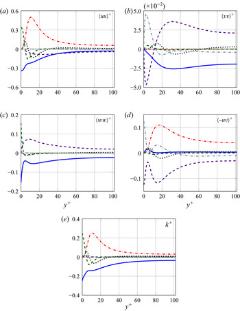
 $L_x = 12 {\rm \pi}h$), the agreement is more than satisfactory. Figure 3 plots all the terms of the single-point budget for each non-zero component of the Reynolds tensor, and for the turbulent kinetic energy
 $k$. In each panel, the residual of the budget is also plotted: the imbalance due to the finite averaging time is negligible, with a maximum of less than
 $1.8\times 10^{-5}$.
Comparison between the present results (coloured lines) and those of Lee & Moser (Reference Lee and Moser2018) (black symbols), obtained at a slightly different  $Re$. (a) Mean velocity profile. (b) Diagonal Reynolds stresses.

Wall-normal profiles of the terms in the budget equation for (a)  $\left \langle {uu} \right \rangle ^+$, (b)
 $\left \langle {vv} \right \rangle ^+$, (c)
 $\left \langle {ww} \right \rangle ^+$, (d)
 $\left \langle {-uv} \right \rangle ^+$ and (e)
 $k^+$. The plots feature the turbulent transport (dotted line), pressure transport (grey dash-dotted line), viscous diffusion (green dashed line), production (red dash-dotted line), pressure strain (purple dashed line) and pseudo-dissipation (blue solid line). The black dashed line plots the imbalance of each equation.

The AGKE terms are computed from the database via a post-processing code that is derived with modifications from its Poiseuille counterpart described by Gatti et al. (Reference Gatti, Chiarini, Cimarelli and Quadrio2020). It also heavily relies on the numerical optimizations introduced by Gatti et al. (Reference Gatti, Remigi, Chiarini, Cimarelli and Quadrio2019) for a precursory GKE version, which computes correlations pseudo-spectrally whenever possible. For maximum accuracy, the derivatives in the homogeneous directions are computed in Fourier space, whereas the derivatives in the wall-normal direction are evaluated by means of a finite-difference scheme with a five-point computational stencil. Since Couette and Poiseuille flows enjoy the same geometrical setting and in particular possess two homogeneous directions, the required modifications to the code from the Poiseuille version only involve changes to statistical symmetries. These changes are listed and discussed in Appendix A. For validation, the residual of the AGKE balance equations is computed to ensure that statistical convergence is reached; it is indeed found to be negligible everywhere in the four-dimensional AGKE space.
3. Results
Perhaps the most prominent feature of turbulent Couette flow is the presence of elongated streamwise counter-rotating vortices which fill the gap between the moving walls. Before describing how these vortices affect the transport processes, the AGKE are used first to characterize these vortices. The analysis serves the dual purpose of discussing similarities and differences between Couette and Poiseuille flows, while demonstrating the effectiveness of the AGKE in discriminating quantitative characteristics of the turbulent structures. Figures comparing Poiseuille and Couette flows are presented when useful; the comparison is carried out with a turbulent Poiseuille flow at  $Re_\tau =200$. Further details of this flow in the context of the AGKE can be found in Gatti et al. (Reference Gatti, Chiarini, Cimarelli and Quadrio2020). Note that such comparison is not unambiguous: owing to the different role of
 $Re$ in the two flows (e.g. Orlandi, Bernardini & Pirozzoli Reference Orlandi, Bernardini and Pirozzoli2015; Andreolli et al. Reference Andreolli, Quadrio and Gatti2021), which Reynolds number should be kept fixed is not established, and the comparison must be intended in a qualitative sense only.
The AGKE are always computed in four-dimensional space  $(r_x,r_y,r_z,Y)$, but in this work results are mostly presented in three-dimensional space with
 $r_x=0$. In fact, the streamwise separation
 $r_x$ is the least significant, because the large vortices are elongated in the
 $x$ direction, thus yielding the maximum correlation at
 $r_x=0$. An important mention of the
 $r_x \ne 0$ case is made in the concluding discussion in § 4.
3.1. The large-scale rolls described via the AGKE
The quantitative characteristics of the large domain-filling streamwise rolls can be most easily identified by the structure function  $\left \langle {\delta u \delta u} \right \rangle$, which is expected to present a maximum (i.e. largest negative correlation) at a spanwise scale
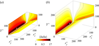
 $r_z$ corresponding to the spanwise vortex size. Figure 4 shows a colourmap for
 $\left \langle {\delta u \delta u} \right \rangle$ drawn on the bounding planes
 $r_y^+=0$,
 $r_z^+=0$ and
 $Y^+=r_y^+/2$ of a box in the
 $(r_z^+,r_y^+,Y^+)$ space, and compares Couette and Poiseuille flows. The domain is bounded by the inclined plane
 $Y^+=r_y^+/2$ owing to the separation
 $r_y$ being constrained by the presence of the wall, i.e.
 $r_y < 2 Y$. The presence of the Couette rolls with their large-scale energy footprint at the wall (Hwang & Cossu Reference Hwang and Cossu2010; Lee & Moser Reference Lee and Moser2018) leads to a change of the position of the structure function maximum, which migrates towards larger spanwise separations. The position of the maximum increases from
 $r_z^+=59$ in Poiseuille flow to
 $r_z^+=183$ in Couette flow. The maximum region is for both flows located close to the wall at
 $Y^+ \approx 20$, and extends for a wide range of spanwise scales. In Couette flow, however, large values of
 $\left \langle {\delta u \delta u} \right \rangle$ are observed up to the channel centre; this is a striking difference from Poiseuille flow, and shows that the footprint of the rolls at the typical large spanwise scale
 $r_z^+ \approx 200$ or
 $r_z \approx 2h$ extends throughout the whole channel. Analogously, the statistical trace of the rolls can be clearly identified also in
 $\left \langle {\delta v \delta v} \right \rangle$,
 $\left \langle {\delta w \delta w} \right \rangle$ and
 $\left \langle {-\delta u \delta v} \right \rangle$ (not shown); Couette flow shows values of the structure functions significantly larger than
 $V_{ij}$ up to the channel core. Table 1 reports value and position of the maxima of each component of the structure function tensor for Couette flow, together with those of other AGKE terms discussed below.
Colourmap of the structure function  $\left \langle {\delta u \delta u} \right \rangle$ in the
 $r_x^+=0$ space for Couette flow (a) and Poiseuille flow (b). The white marker locates the maximum of the structure function.

Maxima of  $\left \langle {\delta u_i \delta u_j} \right \rangle ^+$, source
 $\xi _{ij}^+$, absolute value of the pressure strain
 $|\varPi _{ij}^+|$ and production
 $P_{ij}^+$, and their positions in the
 $(r_y^+, r_z^+, Y^+)$ space for Couette flow.

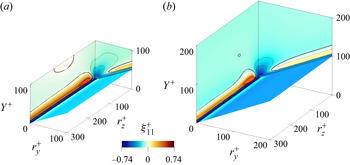
It is interesting to ascertain whether scales and positions where the structure function is largest show net production  $\xi _{11}>0$. Figure 5 plots coloured contours of the source term
 $\xi _{11}$ on the bounding planes, and an isosurface drawn in the volume at
 $75\,\%$ of the maximum. Of particular interest here is the contour line
 $\xi _{11}=0$, discriminating regions and scales where there is net gain of
 $\left \langle {\delta u \delta u} \right \rangle$ from those where there is net loss. Both flows present a region with net gain near the wall in correspondence of the buffer layer, i.e.
 $Y^+ \approx 14$. Term
 $\xi _{11}$ peaks in this region at
 $(r_y^+,r_z^+) \approx (0,40)$ indicating that in both cases the largest production of turbulent fluctuations is associated with the near-wall regeneration cycle (Jiménez & Pinelli Reference Jiménez and Pinelli1999). However, Couette flow features a second region with net positive production (of lower intensity) at the channel centre, at a spanwise scale of
 $r_z^+ \approx 150$. Since the pressure-strain term
 $\varPi _{11}$, shown in figure 6, and the dissipation
 $D_{11}$ (not shown) are negative (almost) everywhere, the local maximum of
 $\xi _{11}$ at the centreline is unequivocally related to the positive production of the large rolls. Indeed, this positive source in the channel core, albeit of limited intensity because of the relatively low
 $Re$, implies that production
 $P_{11}$ is larger than the sum of pressure strain
 $\varPi _{11}$ and dissipation
 $D_{11}$ for
 $r_z^+ \sim 150$. This production at the channel centre is absent in Poiseuille flow, where the anti-symmetry of the mean velocity gradient rules out any production. Interestingly, in Poiseuille flow a second very small positive region can be identified, which is further from the wall but not at the centreline. Although based on this plot alone it might be interpreted as statistical noise, it is known (Gatti et al. Reference Gatti, Chiarini, Cimarelli and Quadrio2020) that this is an early appearance of the outer turbulence cycle, which becomes more and more evident as
 $Re$ increases, but does not extend up to the centreline.
Colourmap of the source term  $\xi _{11}^+$ for Couette flow (a) and Poiseuille flow (b). The colourmap on the bounding planes, with the thick line indicating the contour level
 $\xi _{11}^+=0$, is plotted together with the isosurface
 $\xi _{11}^+=0.55$, which is
 $75\,\%$ of the maximum value.

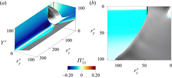
(a) Colourmap of the pressure-strain term  $\varPi _{11}^+$ for Couette flow. The grey isosurfaces mark the boundary of non-preferential energy transfer from streamwise fluctuations towards the others. Inner side:
 $\varPi _{22}^+ > \varPi _{33}^+$. Outer side:
 $\varPi _{22}^+ < \varPi _{33}^+$. (b) A top view and zoom of (a).

A key contributor to the source term is the redistribution provided by the pressure-strain term: figure 6 plots the  $\varPi _{11}$ component as an example. It is (slightly) positive at all scales near the wall, but it is negative everywhere else: the streamwise fluctuations lose energy to feed the cross-stream components at all scales for
 $Y^+>2$. The AGKE visualize at which scales and positions
 $\left \langle {\delta u \delta u} \right \rangle$ is preferentially redistributed towards either
 $\left \langle {\delta v \delta v} \right \rangle$ or
 $\left \langle {\delta w \delta w} \right \rangle$. In figure 6 a grey isosurface is drawn to mark the boundary between the two situations. Following Gatti et al. (Reference Gatti, Chiarini, Cimarelli and Quadrio2020), the isosurface is defined by
 $\varPi _{22}^+ /\varPi _{11}^+ = \varPi _{33}^+ /\varPi _{11}^+ = - 0.5$, with
 $\varPi _{11}^+ < 0$. In the fraction of the volume delimited by the grey isosurface towards the
 $Y^+$ axis, it is found that
 $\varPi _{22}^+ /\varPi _{11}^+ < - 0.5$, hence
 $\varPi _{11}^+$ preferentially redistributes streamwise fluctuations towards the wall-normal fluctuations. This occurs up to the channel centre, where it is true for all
 $r_y^+$ and
 $r_z^+ < 100$ (see figure 6b). On the remaining volume, instead, the preferential receiver of streamwise fluctuation energy is the spanwise component
 $\left \langle {\delta w \delta w} \right \rangle$. A similar picture has already been observed in Poiseuille flow (Gatti et al. Reference Gatti, Chiarini, Cimarelli and Quadrio2020), although here the preferential redistribution to
 $\left \langle {\delta v \delta v} \right \rangle$ takes place within a narrower range of separations.
Note that the structure functions and the net productions peak at similar but not identical positions (see table 1). These differences are discussed in the following.
3.2. The diagonal components of  $\left \langle {\delta u_i \delta u_j} \right \rangle$

We now proceed to study the interscale transfer processes in turbulent Couette flow. As a general observation, the transfers described by Gatti et al. (Reference Gatti, Chiarini, Cimarelli and Quadrio2020) for Poiseuille flow are visible here too: they look nearly identical for  $\left \langle {\delta u \delta u} \right \rangle$ and extremely similar for the other diagonal components. They attest the universality of the near-wall-turbulence cycle for the small scales. Hence, the following discussion is mostly focused on bringing out the role of the large streamwise rolls, which are absent in Poiseuille flow.
The availability of fluxes in the AGKE enables a precise description of the transfer processes through their field lines, which visualize how the fluctuations are transferred among scales and positions. Although energy is not necessarily bound to be continuously transported along these lines, and the flow dynamics may be instantaneously very complex, the fluxes explain the different scales and positions at which  $\left \langle {\delta u_i \delta u_j} \right \rangle$ and
 $\xi _{ij}$ have their peak, and their field lines visualize and help in understanding their spatial arrangement. Figure 7 plots the field lines of the flux vector
 $\boldsymbol {\varPhi }=(\phi _y,\phi _z,\psi )$ for
 $\left \langle {\delta u \delta u} \right \rangle$,
 $\left \langle {\delta v \delta v} \right \rangle$ and
 $\left \langle {\delta w \delta w} \right \rangle$. The lines are coloured by their divergence, i.e.
 $\boldsymbol {\nabla \cdot \varPhi } = \partial \phi _y/\partial r_y + \partial \phi _z/\partial r_z + \partial \psi / \partial Y$, and the colourmap shown in the background is for the corresponding source. While the field lines convey directional information, their colour code is meant to provide quantitative information about their energetic relevance: a positive value of
 $\boldsymbol {\nabla \cdot \varPhi }$ indicates fluxes energized by local mechanisms, while a negative value indicates fluxes releasing energy. Indeed, large positive values of
 $\boldsymbol {\nabla \cdot \varPhi }$ are observed in the vicinity of the points where the lines originate, whereas large negative values are observed in the regions where they vanish.
Field lines of the vector of the fluxes  $\boldsymbol {\varPhi }=(\phi _y,\phi _z,\psi )$ coloured by its divergence
 $\boldsymbol {\nabla \cdot \varPhi }=\partial \phi _y/\partial r_y + \partial \phi _z/\partial r_z + \partial \psi / \partial Y$ for (a)
 $\left \langle {\delta u \delta u} \right \rangle$, (b)
 $\left \langle {\delta w \delta w} \right \rangle$ and (c)
 $\left \langle {\delta v \delta v} \right \rangle$. Colour contours of the corresponding source term are shown on the bounding planes, with a black thick line indicating the zero level. The isosurfaces correspond to
 $75\,\%$ of the source maximum, i.e.
 $\xi _{11}^+=0.55$,
 $\xi _{22}^+= 0.035$ and
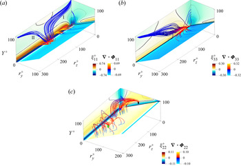
 $\xi _{33}^+=0.07$. In (c), the black dot is the origin of the field lines; the green dot is the singularity point from which other field lines originate.

The fluxes of  $\left \langle {\delta u \delta u} \right \rangle$ are considered first; see figure 7(a). The major contributors to these fluxes are (not shown) the viscous and turbulent transport, with comparable intensity. The field lines of the total flux originating close to the maximum of
 $\xi _{11}$ are analogous to those of the Poiseuille case, and show the same type of transfer; hence they are not discussed here (details can be found in Gatti et al. (Reference Gatti, Chiarini, Cimarelli and Quadrio2020)). However, other field lines point to an additional transfer mechanism at work in Couette flow, which exchanges
 $\left \langle {\delta u \delta u} \right \rangle$ between the near-wall structures and the large streamwise rolls. These lines originate near the wall but just beneath the source maximum in the core, i.e. at
 $(r_y^+,r_z^+,Y^+) \approx (0,200,14)$, at a location in agreement with the peak of the spectral transfer of
 $\left \langle {uu} \right \rangle$, placed by Kawata & Alfredsson (Reference Kawata and Alfredsson2019) at
 $r_z^+=160$ and
 $Y^+=18$ in a Couette flow at
 $Re_\tau =63$. The lines show that part of the excess of
 $\left \langle {\delta u \delta u} \right \rangle$ produced in the near-wall region is transferred towards the channel centre to feed scales and positions associated with the large rolls, indicating a bottom-up interaction. This is highlighted by
 $\boldsymbol {\nabla \cdot \varPhi }_{11}$ which indicates that the fluxes are energized for
 $Y^+ \leqslant 30$ but release energy at larger distances. The rolls are therefore fed by both their own production and the wall turbulence itself. The field lines, once the channel core is reached, are repulsed by the region of positive source. Some lines (collectively referred to as set I) deviate towards the smallest spanwise scales. Others (set II) reach larger
 $r_z$. Figure 8(a,b) describes quantitatively how
 $r_y$,
 $r_z$ and
 $Y$ evolve along a field line of each set, in terms of the normalized position
 $s$ along the line. In the same figure the position(s) along the lines where the divergence of the flux is zero is shown, thus identifying regions where energy is released or received. The excess of
 $\left \langle {\delta u \delta u} \right \rangle$ associated with the spanwise rolls is dissipated both at the smallest scales via the usual direct cascade (set I) and at the large uncorrelated motions via a mixed cascade (set II), in which
 $r_y$ decreases while
 $r_z$ increases. The sink where the lines of set I end is mainly due to viscous effects, whereas along lines of set II energy is lost owing to a combined effect of pressure strain and viscosity.
Evolution of the values of  $r_y^+$ (blue solid line),
 $r_z^+$ (red dashed line) and
 $Y^+$ (green dash-dotted line) along a representative field line for
 $\left \langle {\delta u \delta u} \right \rangle$ set I (a) and set II (b); (c) for
 $\left \langle {\delta w \delta w} \right \rangle$ and (d) for
 $\left \langle {\delta v \delta v} \right \rangle$. The dimensionless arch length
 $s$ is defined as
 $s= 1/s_{max} \int _{0}^{s_{max}}\textrm {d}s$, with
 $\textrm {d}s = \sqrt {\textrm {d}r_y^2 + \textrm {d}r_z^2 + \textrm {d}Y^2}$. The black vertical lines mark the position where the divergence changes sign along the line.

The mutual connection between the near-wall region and the channel core is also evident by looking at the other wall-parallel component  $\left \langle {\delta w \delta w} \right \rangle$. Like
 $\xi _{11}$, the source
 $\xi _{33}$ peaks in the near-wall region at
 $(r_y^+,r_z^+,Y^+)=(0,40,7)$ and has large positive values up to the channel centre at
 $r_z^+ \approx 100$ (see figure 7b). However, in this case the positive source is due to the redistribution of the streamwise component of the turbulent energy via the pressure-strain term, since the production
 $P_{33}$ term is zero as
 $\partial W / \partial y=0$. Unlike for
 $\left \langle {\delta u \delta u} \right \rangle$, all the field lines of
 $\left \langle {\delta w \delta w} \right \rangle$ originate close to the maximum of the source, i.e. at
 $(r_y^+,r_z^+,Y^+)=(12,26,13)$. They are mainly determined (not shown) by the turbulent contribution, the viscous flux being smaller in magnitude. Again, some lines resemble those of Poiseuille flow, vanishing at the smallest scales along the
 $Y$ axis, but others provide a bottom-up transfer of
 $\left \langle {\delta w \delta w} \right \rangle$ from the smaller near-wall structures to the large spanwise rolls. Indeed, figure 8(c) shows that part of the excess of
 $\left \langle {\delta w \delta w} \right \rangle$ near the wall first feeds the large spanwise rolls via an inverse cascade (see the first part of the lines where both
 $r_z$ and
 $r_y$ increase) and then dissipates at
 $r_y \rightarrow 0$ and large
 $r_z$ via a mixed cascade (
 $r_y$ decreases and
 $r_z$ increases); note again that
 $\boldsymbol {\nabla \cdot \varPhi }_{33}$ is positive in the near-wall region and negative away from the wall where the fluxes release energy to the large-scale structures. Overall, a bottom-up transfer of
 $\left \langle {\delta w \delta w} \right \rangle$ is observed together with an inverse cascade followed by a mixed cascade.
Finally,  $\xi _{22}$ too peaks in the near-wall region for scales and positions associated with the near-wall cycle, i.e.
 $(r_y^+,r_z^+,Y^+)=(24,0,31)$, and it is positive up to the channel centre with a local maximum at
 $(r_y^+,r_z^+,Y^+) \approx (120,0,100)$ (see figure 7c). As for
 $\left \langle {\delta w \delta w} \right \rangle$, positive values of
 $\xi _{22}$ mean that
 $\varPi _{22}$ is positive and larger than
 $|D_{22}|$ since the production term of
 $\left \langle {\delta v \delta v} \right \rangle$ is null. Therefore, the pressure strain feeds the vertical fluctuations at both the small near-wall scales and the large scales away from the wall, yielding a net production of
 $\left \langle {\delta v \delta v} \right \rangle$. Field lines at the small scales near the wall are analogous to the Poiseuille case. Lines intercepting larger scales, instead, clearly show a top-down transfer, with scales away from the wall feeding the near-wall structures. The pressure spatial transfer dominates the flux, although viscous scale transfer and turbulent scale transfer play a role at small and large scales respectively. Some lines originate at
 $(r_y^+,r_z^+,Y^+)=(130,60,101)$, a point marked by the black dot in figure 7(c). These fluxes are further energized by the excess of
 $\left \langle {\delta v \delta v} \right \rangle$ in the region with
 $r_y \rightarrow 0$ and larger
 $r_z$, as indicated by the positive
 $\boldsymbol {\nabla \cdot \varPhi }_{22}$. Then they release
 $\left \langle {\delta v \delta v} \right \rangle$ in the near-wall region (
 $\boldsymbol {\nabla \cdot \varPhi }_{22}<0$) and eventually vanish at the wall where
 $\xi _{22}<0$ due to the negative contribution of both the dissipation and (mainly) the pressure strain. The negative
 $\varPi _{22}$ in the vicinity of the wall, together with the positive
 $\varPi _{11}$ (see figure 6) and
 $\varPi _{33}$ (not shown), indicates that the vertical fluctuations turn into wall-parallel ones owing to the splatting effect (Mansour, Kim & Moin Reference Mansour, Kim and Moin1988) present in all wall-bounded flows. Other lines originate from a singularity point at
 $(r_y^+,r_z^+,Y^+)=(120,280,100)$ (green dot in the same figure) where again
 $\xi _{22}>0$. These lines are straight at first with
 $Y$ and
 $r_y$ remaining constant (although figure 7c only shows those going towards lower
 $r_z$), with further energized fluxes; then they reorient towards the wall and become nearly vertical, i.e.
 $r_y$ and
 $r_z$ remain constant, as they are attracted by the sink at the wall. Before vanishing at the wall these fluxes release
 $\left \langle {\delta v \delta v} \right \rangle$ in the near-wall region over a wide range of scales. Overall, the excess of
 $\left \langle {\delta v \delta v} \right \rangle$ produced away from the wall at large
 $r_y$ due to the pressure-strain action feeds a wide range of scales in the near-wall region, where
 $\left \langle {\delta v \delta v} \right \rangle$ is dissipated due to the combined action of pressure strain and viscosity.
Although studying how these statistics change with increasing values of  $Re$ is not the primary concern of this paper, it can be anticipated that the
 $Re$ effects do not qualitatively alter the general picture, since
 $Re_\tau =100$ is already large enough for the outer structures to develop. To confirm this, we have processed a dataset at
 $Re_\tau =500$ taken from Andreolli et al. (Reference Andreolli, Quadrio and Gatti2021); as an example, results for the
 $\left \langle {\delta u \delta u} \right \rangle$ component are provided in figure 9. Figure 9(a) plots the structure function itself. Compared with figure 4(a), the near-wall peak is now accompanied by a visible outer peak at
 $r_z \approx 2h$, and the contours still extend to the centreline. Figure 9(b), to be compared with the plane at
 $r_y=0$ in figure 7(a), portraits fluxes and the source term. The field lines still originate near the wall at
 $r_z \approx 2h$, and proceed towards larger
 $Y$ to give birth to sets I and II. The near-wall maximum of the source is connected to the near-wall cycle and thus scales in wall units, whereas the outer maximum becomes more evident. The source term at low
 $Re$ is dominated by production and its outer maximum is exactly at the centreline, whereas at
 $Re_\tau =500$ the source maximum associated with the outer cycle is found at
 $Y^+ \approx 250$: the large-scale production keeps peaking at the centreline (not shown), but the source term also contains non-negligible contributions from pressure strain, and has its maximum around the scale and the wall-normal distance of the outer cycle.
(a) Results for  $\left \langle {\delta u \delta u} \right \rangle$ at
 $Re_\tau =500$ at
 $r_x=r_y=0$. (b) Field lines of the fluxes of
 $\left \langle {\delta u \delta u} \right \rangle$ coloured with their magnitude, with colourmap of the source term shown in the background (black thick lines indicate the zero level).

In summary, the AGKE reveal an inverse energy cascade for  $\left \langle {\delta u \delta u} \right \rangle$ and
 $\left \langle {\delta w \delta w} \right \rangle$, coupled with an ascending spatial transport that spans the whole domain. On the contrary,
 $\left \langle {\delta v \delta v} \right \rangle$, which is governed by the redistribution term
 $\varPi _{22}$, shows a top-down transport. As discussed later in § 4, this picture partially differs from the description by Kawata & Alfredsson (Reference Kawata and Alfredsson2018), where the diagonal components of the Reynolds stress tensor reportedly present a top-down transfer with a direct cascade only.
3.3. The off-diagonal component $\left \langle {-\delta u \delta v} \right \rangle$

The interaction between the large-scale dynamics and the near-wall turbulence is also observed in the off-diagonal component of the structure function tensor  $\left \langle {-\delta u \delta v} \right \rangle$. Like the single-point quantity
 $\left \langle {-uv} \right \rangle$, this component is not defined in its sign, hence
 $\left \langle {-\delta u \delta v} \right \rangle$ should not be interpreted in terms of energy. The transfer of
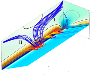
 $\left \langle {- \delta u \delta v} \right \rangle$ is shown in figure 10(a), where field lines of the fluxes are plotted together with the source term
 $\xi _{12}$. Fluxes taking place at scales and positions associated with the near-wall cycle are similar to those of Poiseuille flow and are not discussed here; for clarity the associated lines are not shown in figure 10(a). The remaining field lines are mainly determined (not shown) by the pressure spatial transport, although scale turbulent transport is comparable. Turbulent transport and viscous diffusion are the only non-zero contributions in the scale space, the latter dominating at the small scales and the former at the large scales. The flux lines originate from a straight line placed at large wall-normal distances (
 $Y^+ = 85$ and
 $r_y^+=170$), where
 $\xi _{12}$ is positive, and involve all spanwise separations (to simplify figure 10a, field lines are only plotted for a range of spanwise separations, and a black straight line indicates where they originate). These lines are bound to be tangent to the plane
 $Y^+=h^+$, because the symmetries of the terms involved in the budget equation for
 $\left \langle {- \delta u \delta v} \right \rangle$ imply
 $\psi _{12} = 0$ at the centreline for
 $r_x^+ = 0$ (see Appendix A). Starting from this straight line, some field lines bend and descend vertically towards the wall attracted by the sink
 $\xi _{12}<0$. On the contrary, other field lines direct first towards smaller vertical scales and then descend towards the wall. Overall,
 $\left \langle {-\delta u \delta v} \right \rangle$ is transferred from the central region, where it is maximum, towards the wall region, indicating again that the large rolls interact with the near-wall structures.
Off-diagonal component  $\left \langle {-\delta u \delta v} \right \rangle$. (a) Field lines of the vector of the fluxes
 $(\phi _{y,12}, \phi _{z,12}, \psi _{12})$, coloured by the their divergence and grouped in sets I and II. Colour contours of the source term
 $\xi _{12}^+$ are shown on the bounding planes, with a black thick line indicating the zero contour level. The black straight line placed at
 $Y^+ = 85$ and
 $r_y^+=170$ indicates all the spanwise separations from which some field lines originate. The yellow isosurface corresponds to
 $\xi _{12}^+= 0.09$ The right-hand panel is a zoomed top view of the lines of set II. The evolution of
 $r_y^+$ (blue solid line),
 $r_z^+$ (red dashed line) and
 $Y^+$ (green dash-dotted line) along a representative field line from sets (b) I, (c) II.a and (d) II.b, in which the black vertical lines mark the position where the divergence changes sign along the line.

The lines going towards smaller  $r_y$ can be further divided into two topologically distinct groups, named set I and set II. While reducing their
 $r_y$, the two line sets diverge from each other. Those of set I go towards smaller
 $r_z$ and smaller
 $Y$ being attracted by the region with negative source at
 $r_z^+=0$ (see the dark blue region in figure 10a); at
 $r_z^+ \rightarrow 0$ and small
 $r_y$ they collapse onto a single line that first sticks to the plane
 $r_z^+=0$ and then turns to become a well-defined line at
 $Y^+=50$ and
 $r_z^+=100$. While descending towards the wall, they release
 $\left \langle {-\delta u \delta v} \right \rangle$ as indicated by the negative values of
 $-\boldsymbol {\nabla \cdot \varPhi }_{12}$. Conversely, while reducing their
 $r_y$, lines of set II are repulsed by the positive peak of
 $\xi _{12}^+$ on the
 $r_y^+=0$ plane. Some lines remain at large
 $Y^+$ and release
 $\left \langle {-\delta u \delta v} \right \rangle$ at the smallest scales, ending up on the vertical axis corresponding to zero separations. Most of them, however, release
 $\left \langle {-\delta u \delta v} \right \rangle$ at larger
 $r_z^+$ and lower
 $Y^+$ and eventually vanish at the wall.
Figure 10(b–d) helps in understanding how separations and the wall-normal position change along selected lines of each set. For set I, the transport of  $\left \langle {- \delta u \delta v} \right \rangle$ at first follows the classical energy cascade: the spanwise separation decreases while the transfer takes place from the channel centre towards the wall, until
 $r_z^+ \approx 0$ is reached. In a later stage,
 $r_y^+$ and
 $Y^+$ increase again, and eventually after the turn they become locked at
 $r_y^+=100$ and
 $Y^+=50$, while
 $r_z^+$ increases. For set II, for which a zoom is shown in figure 10(a), the lines of subset II.b simply direct towards the
 $Y^+$ axis to dissipate. Those of subset II.a, instead, show first a continuous decrease of both
 $r_y^+$ and
 $r_z^+$, then the wall-normal separation remains constant at
 $r_y^+ \approx 7$ as
 $r_z^+$ increases, while
 $Y^+$ initially remains constant and reduces afterwards to reach zero value. On such lines an inverse cascade is observed, albeit in a limited range of scales, namely
 $5 < r_y^+ < 10$ and
 $20 < r_z^+ < 135$, while a spatial transfer starts from the channel centre and proceeds towards the wall.
4. Concluding discussion
The transfer of Reynolds stresses has been considered component-wise in a turbulent Couette flow by means of the AGKE, which provide a complete and quantitative description of direct and inverse cascades in the space of scales as well as transfers in the wall-normal direction, for each component of the Reynolds stress tensor. The field lines of the fluxes of Reynolds stresses naturally visualize cascading in physical and scale spaces. When fluxes are observed along the wall-normal direction, top-down and bottom-up processes can be discerned; conversely, when fluxes across scales are considered, direct and inverse cascades are observed. The study builds upon a DNS database, produced for this study at  $Re_\tau = 101.6$, which matches the largest
 $Re$ considered in the experimental study of Kawata & Alfredsson (Reference Kawata and Alfredsson2018). What makes the Couette flow particularly interesting in the present context is its non-zero mean velocity gradient at the centreline, which enables turbulence production, and the presence of large-scale spanwise rolls, whose interaction with the smaller turbulent structures is not entirely understood.
The turbulent Couette flow shows a rich scenario, where direct and inverse cascades coexist, together with bottom-up and top-down interactions. While some of these patterns are also present in plane Poiseuille flow, Couette flow features some peculiarities, which have been addressed by the present study.
The statistical trace of the large rolls is clearly observed in the structure function  $\left \langle {\delta u \delta u} \right \rangle$. In particular,
 $\left \langle {\delta u \delta u} \right \rangle$ is significantly larger than the local covariance in a region encompassing a well-defined spanwise scale of
 $r_z^+ \approx 200$ or
 $r_z \approx 2h$ throughout the whole channel height, with local maxima in the buffer layer and in the core. At the channel centre the source term
 $\xi _{11}$ is positive and quantifies the contribution of the large-scale structures to the overall production; by increasing
 $Re$ the maximum of the source moves towards the wall, because of the relative increased importance of the pressure-strain redistribution, which negatively contributes to the source.
Studying the field lines of the flux vector  $\boldsymbol {\varPhi }=(\phi _y, \phi _z, \psi )$ brings to light the transfer processes among scales and positions. The two wall-parallel components,
 $\left \langle {\delta u \delta u} \right \rangle$ and
 $\left \langle {\delta w \delta w} \right \rangle$, are mainly transferred from the large and small scales near the wall towards larger scales farther away from it. The excess of energy produced near the wall partially feeds the large spanwise rolls, pointing to a scenario of bottom-up transport. In terms of cascade,
 $\left \langle {\delta u \delta u} \right \rangle$ features both direct and inverse cascades, whereas the fluxes of
 $\left \langle {\delta w \delta w} \right \rangle$ reveal the coexistence of an inverse and a mixed cascade. The
 $\left \langle {\delta v \delta v} \right \rangle$ component behaves differently, as expected, and shows a top-down transfer where both inverse and mixed cascades occur. The surplus of
 $\left \langle {\delta v \delta v} \right \rangle$ at the channel core, supplied by the pressure-strain term
 $\varPi _{22}$, is transferred towards the near-wall region via two mechanisms. In the first, small
 $r_z$ scales away from the wall feed near-wall eddies with larger spanwise but lower wall-normal scales. In the second, large
 $r_z$-scale motions placed at the channel core feed near-wall motions over a wide range of scales. The off-diagonal component
 $\left \langle {- \delta u \delta v} \right \rangle$ mainly features a top-down transfer with both direct and inverse cascades, although the inverse one is restricted to a confined range of
 $r_y$ and
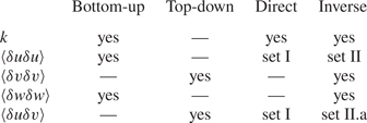
 $r_z$. The dominant transport processes in both the space of scales and in physical space are summarized in table 2.
Types of transport observed in a turbulent Couette flow.

This picture of interscale transfers confirms the conclusions of Kawata & Alfredsson (Reference Kawata and Alfredsson2018), who found an influence of the small near-wall scales upon the large scales away from the wall. However, the present AGKE analysis offers more insight, because of its ability to precisely discriminate the various processes and the scales and positions at which they take place. Some of the extra details brought forward here for the first time are not in agreement with the existing broad picture. Kawata & Alfredsson (Reference Kawata and Alfredsson2018) pointed out that the production of turbulent kinetic energy at large scales is supported by the small near-wall scales by means of the Reynolds shear stress that is transferred from small to large scales throughout the channel. Moreover, they observed a transfer of turbulent kinetic energy from the large scales away from the wall to the small near-wall scales. While the general trend of near-wall scales feeding the large structures at the channel core is confirmed, the present results reveal different space and scale transfers and therefore different sustaining mechanisms. We reveal that the Reynolds shear stress  $\left \langle {-\delta u \delta v} \right \rangle$ is mainly transferred from the large scales in the channel core to the near-wall region, where it is released at both small and large scales. On the contrary, for the turbulent kinetic energy we have described a complex picture, with a bottom-up transfer for the wall-parallel components
 $\left \langle {\delta u \delta u} \right \rangle$ and
 $\left \langle {\delta w \delta w} \right \rangle$, and a top-down transfer for the vertical one
 $\left \langle {\delta v \delta v} \right \rangle$. Thus, the present scenario indicates that the large-scale structures away from the wall are maintained by their production mechanism and by the transfer of the
 $u$ and
 $w$ energy contributions from the large and small near-wall scales respectively. In turn, the large-scale motions away from the wall support the near-wall motions, as shown by the transfers of
 $\left \langle {\delta v \delta v} \right \rangle$, and their production mechanism through the top-down transfer of
 $\left \langle {-\delta u \delta v} \right \rangle$.
Kawata & Tsukahara (Reference Kawata and Tsukahara2021), based on their spectral analysis, provided a schematic model to explain the self-sustaining cycle of the large vortices in Couette flow. The current AGKE analysis confirms the essence of their model, while bringing in some additional details. The model of Kawata & Tsukahara (Reference Kawata and Tsukahara2021) starts by observing that  $\left \langle {uu} \right \rangle$ energy is present at the large scales: this is seen by the positive production at large streamwise scales (figure 10 in their paper), which descends from a positive shear coupled with the positive
 $\left \langle {-uv} \right \rangle$ produced by the large-scale
 $\left \langle {vv} \right \rangle$ (its origin is explained below). Then
 $\left \langle {uu} \right \rangle$ is transferred towards smaller scales as shown by the interscale-transfer term (figure 11 in their paper), following a mechanism described as destabilization of the streaks. At the small scales, the pressure-strain mechanism redistributes
 $\left \langle {uu} \right \rangle$ towards
 $\left \langle {vv} \right \rangle$ and
 $\left \langle {ww} \right \rangle$, and feeds the small-scale streamwise vortices (figure 12 in their paper). Finally,
 $\left \langle {ww} \right \rangle$ is transferred from the small scales to the large scales. Here the pressure strain redistributes
 $\left \langle {ww} \right \rangle$ towards
 $\left \langle {vv} \right \rangle$, leading to a production for
 $\left \langle {-uv} \right \rangle$ and, consequently, for
 $\left \langle {uu} \right \rangle$ at the large scales. The loop is thus closed.
Our analysis is consistent with this view, yet the picture is slightly different and enriched. Figure 11 schematically shows the model of the closed-loop self-sustaining mechanism based on the AGKE results. The main difference is that with the AGKE the transfer among scales at different  $Y$ becomes observable, so that the model can be described as follows. Large
 $\left \langle {\delta u \delta u} \right \rangle$ energy found at
 $r_z^+ \approx 180$ and
 $Y^+ \approx 15$ is the statistical trace of large-scale streaks (see figure 4). They are fed by the mean shear and by the positive
 $\left \langle {-\delta u \delta v} \right \rangle$, associated with the large-scale rolls and released from the fluxes at these large spanwise separations close to the wall. The excess of
 $\left \langle {\delta u \delta u} \right \rangle$ associated with the streaks is transferred to both larger and smaller scales, as well as both towards and away from the wall, by the combined action of viscous diffusion and turbulent transport. The most part is transferred away from the wall (see figure 7a), where pressure strain redistributes
 $\left \langle {\delta u \delta u} \right \rangle$ towards the cross-stream components. Hence, these transfers and the pressure-strain activity explain how the large-scale streaks feed the large-scale vortices. The fluxes of
 $\left \langle {\delta w \delta w} \right \rangle$ (figure 7b) indicate that the spanwise fluctuations of the large spanwise rolls are fed not only by the pressure-strain redistribution, but also by the near-wall cycle. At large
 $Y$ and large
 $r_z$ the large
 $\left \langle {\delta v \delta v} \right \rangle$ together with the mean shear generate positive production for
 $\left \langle {-\delta u \delta v} \right \rangle$. The produced
 $\left \langle {-\delta u \delta v} \right \rangle$ is then transferred towards the wall via pressure transport, and part is released by the fluxes at
 $r_z ^+ \approx 150$ (set II.a in figure 10). The resulting positive
 $\left \langle {-\delta u \delta v} \right \rangle$, together with the mean shear, is responsible for
 $P_{11}>0$ thus sustaining the large-scale streaks. The loop is thus closed.
Schematic model of the closed-loop sustaining mechanism for  $\left \langle {\delta u_i \delta u_j} \right \rangle$ in the
 $r_x=0$ space, associated with the large-scale motions.

Although so far the streamwise separation has not been considered, it must be said that concerns have been recently raised on the conclusions derived from such partial observations neglecting streamwise separations/wavenumbers. For example, Kawata & Tsukahara (Reference Kawata and Tsukahara2021) found via a spanwise Fourier mode analysis that an inverse transfer of  $\left \langle {uu} \right \rangle$ is still present when the computational domain is restricted in its spanwise size to remove the outer structures. Hence, such a mechanism would not represent an interaction between the near-wall cycle and the large outer structures, as confirmed by the absence of an inverse cascade in the analysis of the streamwise Fourier modes. They suggested that this may be related to the self-sustaining cycle of the inner and/or outer structures. To address this point, we show in figure 12 fluxes for
 $\left \langle {\delta u \delta u} \right \rangle$ and
 $\left \langle {\delta w \delta w} \right \rangle$ in three-dimensional space at
 $r_y=0$, which considers the streamwise separation too.
Field lines of the vector of the fluxes in the  $(r_x^+, r_z^+, Y^+)$ space for
 $\left \langle {\delta u \delta u} \right \rangle$ (a) and
 $\left \langle {\delta w \delta w} \right \rangle$ (b). Colour contours of the corresponding source term are shown on the bounding planes. The flux lines are coloured with the flux magnitude.

For  $\left \langle {\delta u \delta u} \right \rangle$ the lines associated with the large scales originate at
 $r_x=0$, and thus their starting point is the same as in the
 $r_x=0$ space. They develop both close to the wall and at larger
 $Y$; streamwise energy is transferred via both direct and inverse cascades. These lines can thus be interpreted, as done in the previous analysis with
 $r_x=0$, as part of the self-sustaining cycle of the large-scale rolls. The lines of
 $\left \langle {\delta w \delta w} \right \rangle$ confirm that they initially possess small spanwise separations (much like in the channel flow) and then move towards large
 $r_z$ and large
 $Y$, indicating again an interaction of the small scales of the near-wall cycle with the large spanwise rolls located away from the wall. Thus, looking at
 $r_x = 0$ already seems to provide the correct picture, and suggests that
 $\left \langle {\delta u \delta u} \right \rangle$ is driven by an autonomous large-scale mechanism and the transfers of
 $\left \langle {\delta w \delta w} \right \rangle$ describe an interaction between the near-wall cycle and the large outer structures.
The present analysis has mostly considered a single, relatively low value of the Reynolds number, and thus its extension to higher  $Re$ remains interesting and useful. Nevertheless, already at this
 $Re$, because of their capability of properly defining the concept of scale in the wall-normal direction and of providing a detailed view of each component of the Reynolds stress tensor, the AGKE have been essential to understand and describe the interaction between the near-wall turbulence and the elongated rolls of turbulent Couette flow.
Acknowledgements
The authors acknowledge computing support by the state of Baden-Württemberg through bwHPC. D.G. acknowledges partial support by the Priority Programme SPP 1881 Turbulent Superstructures of the Deutsche Forschungsgemeinschaft.
Funding
This research received no specific grant from any funding agency, commercial or not-for-profit sectors.
Declaration of interests
The authors report no conflict of interest.
Appendix A. Symmetries
The symmetries in the terms of the AGKE are listed below for the case of plane Couette flow.
The terms appearing in the budget equations of  $\left \langle {\delta u \delta u} \right \rangle$,
 $\left \langle {\delta v \delta v} \right \rangle$,
 $\left \langle {\delta w \delta w} \right \rangle$ and
 $\left \langle {\delta u \delta v} \right \rangle$ are first considered. The inversions of
 $\boldsymbol {r}$ and of the spanwise coordinate
 $z$ lead to the same symmetries as in Poiseuille flow (Gatti et al. Reference Gatti, Chiarini, Cimarelli and Quadrio2020). Inversion
 $\boldsymbol {r} \rightarrow -\boldsymbol {r}$ leads to
 $\boldsymbol {\phi } \rightarrow -\boldsymbol {\phi }$,
 $\psi \rightarrow \psi$,
 $\xi \rightarrow \xi$ and
 $\left \langle {\delta u_i \delta u_i} \right \rangle \rightarrow \left \langle {\delta u_i \delta u_i} \right \rangle$;
 $z \rightarrow -z$ implies
 $r_z \rightarrow -r_z$ and consequently
 $\phi _x \rightarrow \phi _x$,
 $\phi _y \rightarrow \phi _y$,
 $\phi _z \rightarrow - \phi _z$,
 $\psi \rightarrow \psi$,
 $\xi \rightarrow \xi$ and
 $\left \langle {\delta u_i \delta u_i} \right \rangle \rightarrow \left \langle {\delta u_i \delta u_i} \right \rangle$. On the contrary, the inversion of the wall-normal coordinate
 $y$ leads to different symmetries compared with Poiseuille flow, as it implies also the inversion of the streamwise coordinate
 $x$. It leads to
 $Y \rightarrow -Y$,
 $r_x \rightarrow -r_x$,
 $r_y \rightarrow -r_y$ and consequently
 $\phi _x \rightarrow - \phi _x$,
 $\phi _y \rightarrow - \phi _y$,
 $\phi _z \rightarrow \phi _z$,
 $\psi \rightarrow - \psi$,
 $\xi \rightarrow \xi$ and
 $\left \langle {\delta u_i \delta u_i} \right \rangle \rightarrow \left \langle {\delta u_i \delta u_i} \right \rangle$.
The terms involved in the budget equations of  $\left \langle {\delta u \delta w} \right \rangle$ and
 $\left \langle {\delta v \delta w} \right \rangle$ are now considered. In comparison with the other components, their symmetries are the same for an inversion of
 $\boldsymbol {r}$ but differ when the inversions of
 $z$ or
 $y$ (and
 $x$) are considered. When
 $z$ is inverted the AGKE terms undergo
 $\phi _x \rightarrow - \phi _x$,
 $\phi _y \rightarrow - \phi _y$,
 $\phi _z \rightarrow \phi _z$,
 $\psi \rightarrow - \psi$,
 $\xi \rightarrow - \xi$ and
 $\left \langle {\delta u_i \delta u_i} \right \rangle \rightarrow -\left \langle {\delta u_i \delta u_i} \right \rangle$, as in Poiseuille flow. The inversion of
 $y$ (and
 $x$) leads to
 $\phi _x \rightarrow \phi _x$,
 $\phi _y \rightarrow \phi _y$,
 $\phi _z \rightarrow - \phi _z$,
 $\psi \rightarrow \psi$,
 $\xi \rightarrow - \xi$ and
 $\left \langle {\delta u_i \delta u_i} \right \rangle \rightarrow -\left \langle {\delta u_i \delta u_i} \right \rangle$ for
 $\left \langle {\delta u \delta w} \right \rangle$ and
 $\left \langle {\delta v \delta w} \right \rangle$.
Overall, these symmetries imply that some terms of the AGKE are zero in particular regions of the four-dimensional domain. These regions (except the trivial case of  $\boldsymbol {r}=\boldsymbol {0}$) are listed below for each component
 $\left \langle {\delta u_i \delta u_j} \right \rangle$. For notational simplicity the origin of the wall-normal coordinate is shifted to the centreline of the channel.
For  $\left \langle {\delta u \delta u} \right \rangle$,
 $\left \langle {\delta v \delta v} \right \rangle$,
 $\left \langle {\delta w \delta w} \right \rangle$ and
 $\left \langle {\delta u \delta v} \right \rangle$:
 \begin{equation} \left.\begin{gathered} \phi_x(Y,0,0,r_z) = 0, \\ \phi_y(Y,0,0,r_z) =0, \\ \phi_z(Y,r_x,r_y,0) = 0, \\ \psi(0,r_x,r_y,r_z) =0. \end{gathered}\right\} \end{equation}
For  $\left \langle {\delta u \delta w} \right \rangle$ and
 $\left \langle {\delta v \delta w} \right \rangle$:
 \begin{equation} \left.\begin{array}{cc@{}}
\phi_x(Y,r_x,r_y,0) =0, & \\ \phi_y(Y,r_x,r_y,0)
=0, & \\ \phi_z(Y,0,0,r_z) =0, & \\
\psi(Y,r_x,r_y,0) =0, &
\psi(Y,0,0,r_z)=0, \\ \psi(0,r_x,r_y,r_z)
=0, & \\ \xi(Y,r_x,r_y,0) =0, &
\xi(Y,0,0,r_z)=0, \\ \left\langle {\delta u_i
\delta u_j} \right \rangle(Y,r_x,r_y,0) =0, &
\left\langle {\delta u_i \delta u_j} \right
\rangle(Y,0,0,r_z)=0. \end{array}\right\}
\end{equation}