The election forecasts presented in this article indicate that control of the White House after the 2012 election is a tossup, that control of the US House will likely remain in Republican hands, and that although closely fought, the Republicans have the edge for control of the US Senate. These forecasts were made on July 15, 2012. Obama was predicted to receive 51.3% of the two-party popular vote, 301 electoral votes, and to have a 57.1% chance of winning the Electoral College. The year 2012 was forecast to be one of stasis for the US House, with almost no change in the number of seats controlled by the Republicans: they were forecast to pick up two seats, and to have a 75.6% chance of maintaining their majority. Lastly, the Republicans were predicted to pick up five seats in the US Senate and have about a 61.6% chance of attaining majority control.
PREDICTION MODELS
These forecasts were made by analyzing the relationship between prior election outcomes and causal factors that can be measured before elections. Then, the values of these causal factors in 2012 were used in conjunction with the strength of the relationships in the past to make forecasts for the 2012 election. Accordingly, the dependent variable in the following four models was the percentage of the two-party vote going to the Democrats in the presidential, US Senate, US House, or gubernatorial elections, using the years from 1948 to 2010.Footnote 1 The predictor variables used for these models followed the forecasts of Klarner (Reference Klarner2008) with some alterations mentioned later in the text. Space constraints preclude theoretical justification for the independent variables, but this justification has been described elsewhere (Klarner Reference Klarner2008), and all have been used by multiple scholars (see, for example, Abramowitz Reference Abramowitz2008).
The strength of statistical models as a method of forecasting elections is that they give more insight into why an election turned out the way it did than do forecasting methods that are based on expert judgments or the Iowa Electronic Market. In statistical models, it is tempting to use predictors that ask people how they will vote in the upcoming election. However, we gain little insight into why an election turned out the way it did because that was how most people said they were going to vote three months before Election Day.Footnote 2 Accordingly, vote intention variables are not used here, unlike in Klarner (Reference Klarner2008).
The difference between the forecasting models presented here and most others is that the state-year is the unit of analysis, allowing state-level forecasts (but see Campbell, Ali, and Jalalzai Reference Campbell, Ali and Jalalzai2006). Klarner (Reference Klarner2008) used the district-year as the unit of analysis for the US House of Representatives prediction models, but redistricting complicated making district level forecasts for 2012. This unit of analysis was changed partly because lagged vote share mapped to 2012 US House districts were not available, but, more importantly, because past vote share may have a fundamentally different impact in elections after redistricting. Hierarchical linear modeling was used, with a level-2 error term at the year level, which took into account aspects of the partisan wave that were not captured by the national-level variables described in this article. After the models were run, Monte Carlo simulation was used to compute the probability of various national-level outcomes, such as the probability that Obama or Romney would win a majority in the Electoral College.
Cuzán and Burdick (Reference Cuzán and Burdick2009) identified major problems with basing election forecasts on limited numbers of cases. Because using pooled cross-section time-series data considerably increases the number of cases for analysis, these datasets may side-step this problem. The availability of so many cases for analysis also allows the use of lagged independent variables, which more fully capture the dynamics of the phenomena being forecast (De Boef and Keele Reference De Boef and Keele2008). For models with the US Senate, variables were lagged in terms of the last election for a particular class of senator in a state, unlike in Klarner (Reference Klarner2008). Another alteration from Klarner (Reference Klarner2008) was that lagged independent variables were included whether or not these attained statistical significance. Finally, missing data were not imputed with a missing data algorithm, unlike in Klarner (Reference Klarner2008).
State-years with uncontested elections were not used in the relevant model.Footnote 3 To take into account the fundamentally different nature of states in the “solid South,” state-years were excluded from analysis when more than 84% of its state-house members were of a particular major party in the prior year. State-years were also excluded for a particular office if a nonmajor party candidate received more votes than either major party candidate, received more than 25% of the vote, or was an incumbent.
The variables used to predict election outcomes can be put into four general categories: candidate attribute, partisan disposition, national level, and state level.
Candidate Attribute
For the presidential model, one candidate attribute variable measured whether a state was the home state of the Democratic (coded “1”) or Republican (coded “−1”) presidential candidate (coded “0” otherwise), along with an analogous variable for vice presidential candidates.
Candidate attribute variables for the US House measured the percent of Democratic candidates in a state and year who possessed a particular characteristic, subtracted by the percent of Republican candidates who possessed that characteristic. Such variables measured the percent of seats that (1) were uncontested by a party, (2) had an incumbent, (3) had an unelected incumbent, (4) had a nonincumbent who held an elective position currently or in the past, and (5) had a nonincumbent candidate who was a former US House member.Footnote 4 Incumbents who are more moderate in their roll-call voting behavior have been found to garner more votes than those who are less moderate. Accordingly, the average of Keith Poole's first-dimension DW-Nominate scores for the incumbents in a state who were running for reelection was included, where higher values indicated more conservative voting. An interaction between this variable and the percent of seats in a state in which an incumbent was running was also included, as average DW-Nominate scores would be more influential the greater the proportion of elections in which incumbents were running.Footnote 5
For the US Senate and gubernatorial elections, candidate attribute variables were coded “1” when the Democratic candidate had the attribute in question and “-1” when the Republican did. These measured (1) whether the prior election was uncontested, (2) incumbency, and (3) unelected incumbency. A five-point elective office holder scale was also used for nonincumbents, with negative values for Republicans.Footnote 6 The DW-Nominate scores of incumbent senators were also included.
Partisan Disposition
Numerous variables were used to measure the partisan disposition of a state. The first variable was the lagged dependent variable for the relevant type of election. The lagged election returns of three other offices—centered around the average for the year in which they were measured—were also used to measure the partisan disposition of a state. These were the Democratic percent of the two-party vote for president and US House, as well as the percent of major-party state house legislators who were Democrats. Centered presidential returns were not used for the presidential model, and centered US House returns were not used for the US House model.
National Level
The national level variables were as follows. A two-term penalty variable was included in the presidential model, coded “1” when a Democrat had been in the White House for two terms or more, “−1” for such Republican administrations, and “0” in other years (Abramowitz Reference Abramowitz2008). For the other three models, a midterm penalty variable was used, coded “1” in nonpresidential years when a Democrat was in the White House, “−1” in such years with a Republican administration, and “0” in presidential election years.
Two national level variables were utilized in all models: First, the percent approving of the job of the president in the Gallup Poll was measured as close as possible to 129.5 days before the election.Footnote 7 This variable was multiplied by “−1” when a Republican was in the White House. Because of this multiplication, a variable coded “1” when the president was a Democrat and “−1” when the president was a Republican was also included. A second national level variable used in all models measured the health of the economy. Many forecasting models have used gross domestic product to measure the health of the economy, but real personal income is a more theoretically sound way to measure the electorate's economic well-being (Bartels and Zaller Reference Bartels and Zaller2001). Accordingly, the health of the national economy was measured by the percent change in real disposable income from July of the year prior to the election to May of the election year.Footnote 8 This variable was also multiplied by “-1” when a Republican was in the White House.
State Level
Only one aspect of state conditions was used: state economic growth. This was measured by the percent change in real disposable income from the third quarter of the calendar year prior to the election to the first quarter of the election year. In all models, this was multiplied by “−1” when a Republican was in the White House. In the gubernatorial models, an additional variable which represented an interaction between state economic growth and the party of the governor (with a Republican governor coded “−1” and a Democratic governor coded “1”) was included to take into account the possibility that the electorate holds governors responsible for state economic growth.
As explained earlier, all independent variables were lagged. With only 16 election years available for analysis in the presidential model, multicollinearity was a problem for the national level variables, so no lagged national-level variables were used. The lagged midterm loss variable had to be excluded for the US House because it was perfectly collinear with other variables. Lagged independent variables were expected to have the coefficient opposite in sign of their nonlagged counterparts.
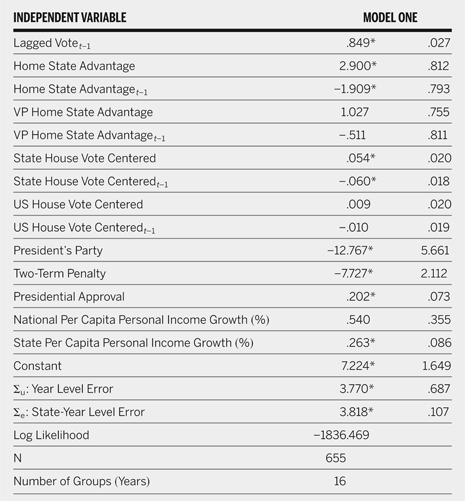
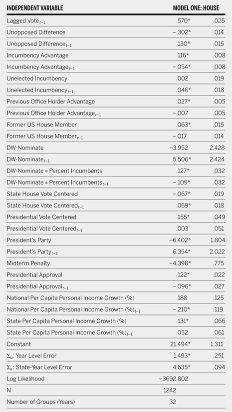
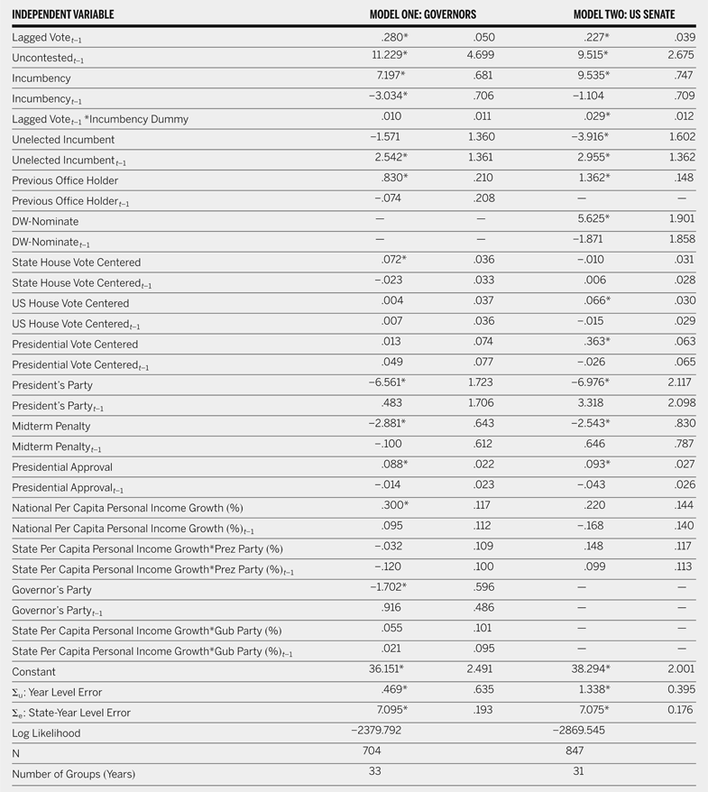
Table 1 displays the findings for the presidential model, table 2, for the US House model, and table 3, for the gubernatorial and US Senate models. The majority of variables behaved as expected and were statistically significant. Due to space constraints, no comments about the findings of the models are published here.
Determinants of State Level Democratic Vote: Presidential Elections, 1948–2008

Note: The dependent variable is the percentage of the major-party vote obtained by Democrats in a state-year. Cell entries are the unstandardized random-effects ML regression coefficient, followed by its standard error in the last column. Random effects are grouped by year.
* p < .05, one-tailed test.
Determinants of State Democratic Vote: US House, 1948–2010

Note: The dependent variable is the percentage of the major-party vote obtained by Democrats in a state-year. Cell entries are the unstandardized random-effects ML regression coefficient, followed by its standard error in the last column. Random effects are grouped by year.
* p < .05, one-tailed test.
Determinants of State Democratic Vote: Gubernatorial (1946–2010) and US Senate (1950–2010) Elections

Note: The dependent variable is the percentage of the major-party vote obtained by Democrats in a state-year. Cell entries are the unstandardized random-effects ML regression coefficient, followed by its standard error in the third and fifth columns. Random effects are grouped by year.
* p < .05, one-tailed test.
TRANSLATION OF VOTES INTO SEATS FOR THE US HOUSE
The translation of votes into seats at the state level for the US House was also necessary to model. When a state had only one congressional district, the translation of votes into seats was simply determined by which party had a majority of the two-party vote in one of the 2,000 simulations. For all other states, prediction models with the following independent variables were used. The first was the Democratic percent of the two-party vote in a state. The second and third were variables representing the percent of seats in a state that had a Republican (Democratic) incumbent. Given the same percentage of votes in a state for a party, we would expect a party to obtain more seats the more incumbents they have running. The fourth and fifth variables represented the percent of seats for which the Republicans (Democrats) did not run a candidate. Given two states with the same percent of Republican votes, we would expect the Republicans (Democrats) to win more seats in a state where they ran fewer candidates.
Ordered logistic regression was used for predicting the number of seats won by Democrats in states with two congressional districts. For states with three or more congressional districts, ordinary least squares was used as it was found to be as effective at predicting seats as ordered logistic regression. The dependent variable in these models was the percent of seats in the state won by the Democrats. States were divided into four categories for analysis based on their number of districts (3–5, 6–8, 9–13, and 14–53). For brevity, the results of these five models are not displayed here.Footnote 9
Variables that measured partisan control of the redistricting process were not included. However, prior scholarship finds little partisan bias in redistricting (Friedman and Holden Reference Friedman and Holden2009). Furthermore, because incumbency was controlled for, the impact of redistricting through retirements and forcing two or more incumbents to face off in the same congressional district was taken into account. Furthermore, the impact of reapportionment is considered.
SIMULATIONS
After the models described here were run, the values of all independent variables were measured in 2012, and the coefficients and standard errors associated with those variables displayed in tables 1, 2, and 3 were used to generate estimated values at the state level for 2012 in the manner described in the following text.Footnote 10 A second stage of simulations was carried out for the translation of votes into seats for the US House.
For the first stage of simulations, election outcomes were generated 2,000 times. It is not justified to take the estimated values generated from independent variables' coefficients and then add a random quantity to this estimated value with the standard deviation matching the standard error of the estimate. For out of sample predictions, the uncertainty associated with each independent variables' coefficient must also be considered (Beck Reference Beck, Campbell and Garand2000). As a result, for each of the 2,000 simulations, a normally distributed random variable with a mean of zero and a standard deviation reflecting the standard error of each coefficient was added to each coefficient. Then, these were multiplied by the values of the independent variables in 2012 and added together to yield predicted values. Next, these quantities were added to two random variables: one that varied across all states in one simulation which also had a standard deviation that matched the level-1 error term, and another that was constant across all states in one simulation, which also had a standard deviation that matched the level-2 error term.Footnote 11 The next step in the presidential and US Senate models was to recode each state as being won by the Democrats or Republicans, and then summing up the number of electoral votes or Senate seats for the Democrats for each of the 2,000 simulations. The popular vote for the presidency was computed by weighting Democratic vote share by the number of major party votes in a state in the prior election.Footnote 12
For the translation of votes into seats for the US House, the percent of the vote for the Democrats in a state from each of the 2,000 simulations was put into the second-stage simulation model, and then analogous simulations to those described earlier were done. If the number of seats predicted from one of the 2,000 simulations was out of bounds on the basis of the number of a state's congressional districts and uncontested elections, these were brought to the minimum or maximum bound of the possible range as appropriate.
A “drop one year” analysis was conducted for the presidency. In this analysis, one election year from the presidential dataset was dropped in turn, and the model described earlier for all election years was run on the remaining years. Then, estimated values for each state were computed for the omitted year, and the national popular vote was computed by a weighted average, with weights equal to the number of major party votes from the last election. Next, these were compared with the actual popular vote, but only for states that were not excluded from the analysis (i.e., not the solid South). Subtracting the actual from the forecast percent of the Democratic two-party popular vote yielded the following for each year (positive numbers indicate a pro-Republican bias in the forecast): 1948 (7.1), 1952 (7.5), 1956 (5.5), 1960 (3.3), 1964 (8.7), 1968 (−6.4), 1972 (−7.2), 1976 (5.8), 1980 (−9.1), 1984 (2.8), 1988 (.6), 1992 (−2.4), 1996 (1.0), 2000 (.0), 2004 (−1.4), 2008 (−5.3). These numbers imply uncertainty bounds that are smaller than those created by the Monte Carlo simulation presented later in the text, which imply that the simulation method described earlier may be too strict. Second, the presidential model presented in Klarner (Reference Klarner2008) was altered in ways that many scholars might consider to be insubstantial. Yet for the 2008 election, Klarner (Reference Klarner2008) forecast that Obama would get 53.0%, while the “drop one year” analysis resulted in a prediction of 58.6%. This illustrates that political scientists should put renewed emphasis on justifying modeling decisions that many might believe are small ones.
FORECASTS
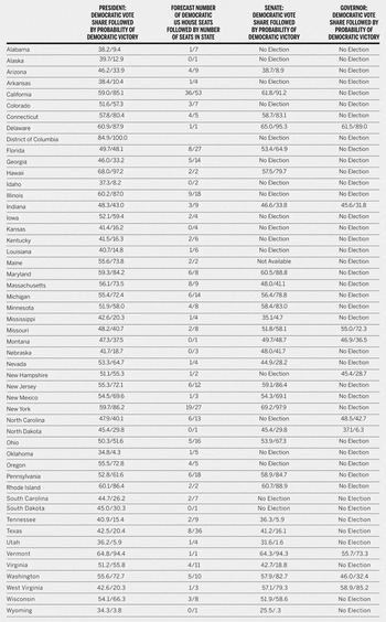
The following forecasts were finalized on July 15, 2012. The simulations indicated that there was a 57.1% chance of a Democratic victory in the Electoral College, with a .1% chance of a tie. Obama was forecast to receive 301 electoral votes, the median number of electoral votes across the 2,000 iterations. The simulations indicated a great deal of uncertainty about the outcome, with a 95% confidence interval of 7 to 526 electoral votes for the Democrats, and a 66.7% confidence interval of 119 to 450. The median estimate from the simulations of the Democratic percentage of the two-party popular vote was 51.3%, with a 95% confidence interval of 34.9 to 67.0%, and a 66.7% confidence interval of 43.4% to 59.3%. The probability of Obama being the Electoral College winner but popular vote loser was 2.5%, while the probability of that happening to Romney was 1.9%. Table 4 displays forecasts at the state level for all four offices. Florida and Ohio were forecast to be tossups between Obama and Romney, with Obama predicted to receive 49.7% and 50.3% of the vote, respectively. This forecast provides insight into why there was so much uncertainty about the overall outcome. Although not as closely fought, Pennsylvania was predicted to yield 52.8% for Obama. Numerous medium-sized states were also predicted to be closely fought, including Colorado, Indiana, Iowa, Minnesota, Missouri, North Carolina, and Virginia.Footnote 13
State Level Forecasts

Simulations for the US House indicated there was a 75.6% chance the Republicans will keep majority control. The median estimate from the simulations was that the Democrats would be left with 191 seats after the election, a decrease of two seats from their current 193. Again, the margin of error from the simulations was very large, with a 95% confidence interval of 115 to 270 Democratic seats, and a two-thirds confidence interval going from 153 to 228 Democrats.
The forecasting models here did not consider the impact of large nonmajor party candidacies, although Sanders (VT) was treated as a Democrat for the analysis and forecasts. Because Angus King, former independent governor of Maine, was running for the US Senate, no forecast was made for that state, leaving 32 states with forecasts.Footnote 14 The results of the US Senate forecasting model and simulations indicated that the Democrats will win 18 of the 32, implying the Republicans will pick up five seats, as the Democrats hold 23 of those that are up for election.Footnote 15 Of the seats not up for election, Democrats hold 30, meaning they were predicted to be left with 48 seats, causing them to lose majority control. Of course, the necessary number of senators for majority control is contingent on the party of the vice president. Accordingly, the simulations indicated there was a 42.0% chance the Democrats will have 50 seats or more, and a 33.6% chance they will have 51 seats or more.Footnote 16 Together with the probability of the Democrats winning the presidency cited earlier, this implied that the Democrats had approximately a 38.4% chance of retaining control of the Senate.Footnote 17 Another contingency is that Angus King will caucus with the Democrats, and the Democrats win the presidency, meaning they need 49 seats or more for majority control. In that contingency, there is a 49.8% chance the Democrats will have majority control.
Last, table 4 indicates that the simulations predicted easy Democratic victories in the Delaware and West Virginia gubernatorial elections, and a clear Republican victory in North Dakota. Missouri and Vermont are leaning Democratic victories, while Indiana, Montana, New Hampshire, and Washington are leaning Republican. North Carolina is highly competitive with a 42.7% chance of a Democratic victory.
Overall, the 2012 elections promise to be highly competitive ones, with control of both the presidency and US Senate within the grasp of both of the major parties, and only the outcome for the US House predicted to be one of constancy.