GOVERNMENT SURVIVAL

As comparativists may recall, beginning in the 1970s and extending through the 1990s, the literature on government durability was dominated by debate between the “attributes” and “events” approaches to the question.Footnote ² In short, the attributes approach conceived of government durability as a function of characteristics which can be observed at the time of the cabinet’s formation (e.g., Warwick Reference Warwick1979; Strøm Reference Strøm1985). That is, governments in general are made more durable by activating certain features (majority status, for example) and coalition governments, in particular, can be made more stable by selecting partners that are compatible on salient policy dimensions. The events approach, by contrast, argued that cabinet stability is primarily a function of stochastic shocks to the political environment (e.g., Browne, Frendreis, and Gleiber Reference Browne, Frendreis and Gleiber1984). Warwick (Reference Warwick1994) provides a thoughtful and detailed discussion of this debate.

The rift between these competing perspectives eventually gave way to an acceptance that both attributes and events were salient to government longevity and that researchers must integrate both into a hybrid model that considers how cabinets’ characteristics make them more or less likely to survive the various shocks they may experience, or, how certain shocks may have the potential to reshape the properties of the status quo government relative to its alternatives. The incorporation of the two approaches into a unified framework is now the dominant theoretical perspective on government stability and exemplified by Lupia and Strøm (Reference Lupia and Strøm1995), Laver and Shepsle (Reference Laver and Shepsle1998), and Diermeier and Stevenson (Reference Diermeier and Stevenson2000), who argue that the relevant “events” are shocks to the political environment that alter the distribution of bargaining power across legislative parties, making alternatives to the status quo government more or less attractive, and therefore making termination more or less likely.

These theoretical innovations went hand-in-hand with empirical advances that sought to model the attributes or events approaches separately (e.g., Strøm Reference Strøm1985; Browne, Frendreis, and Gleiber Reference Browne, Frendreis and Gleiber1986, respectively), before moving on to harmonize them. One could argue that, in this respect, the empiricists were a step ahead of the theorists, with King et al. (Reference King, Alt, Burns and Laver1990, 847; authors’ emphasis) presenting a “statistically unified model that can be used to explore the impact of particular attributes upon cabinet durability (expected duration), while maintaining the assumption that the duration of any particular cabinet will ultimately be determined by a stochastic process, such as the random incidence of terminal events”—a model that correctly predicts government duration within four months on average.

This is not the case in regard to the next major hurdle in the literature: recognizing, and subsequently modeling, the selection problem in cabinet durability. As early as De Swaan (Reference De Swaan1973), theorists had understood that durability was a critical concern in the formation of governments, but it would be several decades until empiricists began to engage this issue in earnest (e.g., Merlo Reference Merlo1997; Diermeier, Eraslan, and Merlo Reference Diermeier, Eraslan and Merlo2003) and later still before a solution to the selection problem was proposed to jointly model formation and duration by Chiba, Martin, and Stevenson (Reference Chiba, Martin and Stevenson2015), who find significant differences between the correlates of durability when selection is and is not accounted for. In the interim, we have learned that a government’s durability is a function of events and attributes such as majority status, the complexity of the bargaining environment, the number and size of antiestablishment parties in parliament, and ideological compatibility within the government, though the findings of Chiba, Martin, and Stevenson (Reference Chiba, Martin and Stevenson2015) suggest previous estimates of the salience of compatibility may have been overstated as a function of the aforementioned selection bias.Footnote ³ Importantly, the presence of selection bias provides evidence that cabinets can and do forecast their durability.

What all of this research (and scores of books and articles we have not discussed) has in common is its consistent attention to durability as the dependent variable.Footnote ⁴ Even when the theoretical focus is not attributes of the cabinet itself, but on alternative political economic phenomena, like, for example, natural resource revenue or interstate transfers, incumbent duration is still nearly always found on the left-hand side of the equation (e.g., Ahmed Reference Ahmed2012; Bueno De Mesquita and Smith Reference Bueno De Mesquita and Smith2010). This is likely because most scholars perceive the importance of cabinet longevity as self-evident, and on this we do not disagree. Nevertheless, the overwhelming focus on duration as a dependent variable has obscured why scholars were moved to study it in the first place: the belief that rapid government turnover is, on some normative level, a net negative, or at the very least salient to democratic representation and governance. That is, the entirety of this literature is motivated by the assumption that cabinet stability has powerful implications for, in the words of King et al. (Reference King, Alt, Burns and Laver1990, 846), “democratic stability, policy continuity, or even executive dominance over the legislature” among numerous other, more specific, substantively interesting and normatively significant political economic outcomes. However, in the political science literature, we could find only two empirical studies making a robust connection between cabinet stability, as an independent variable, and democratic outcomes (broadly defined)—one links government instability (in terms of executive turnover) to decreased levels of overall satisfaction with democratic governance (Harmel and Robertson Reference Harmel and Robertson1986) and the other finds that short-term spikes in portfolio volatility decrease the efficiency of policy implementation (Huber Reference Huber1998).Footnote ⁵

All of this is to say that, while the supply of research devoted to understanding the causes of government durability is vast and deep, the supply of empirical research devoted to understanding the consequences of government durability is nearly nonexistent. As such, whether or not cabinet stability actually bears any real policy consequences remains an almost entirely open question, one that we begin to provide an answer to by assessing the relationship between government longevity and public spending—perhaps the most significant policy decision that governments must make.

PUBLIC SPENDING

Interest in public spending in political economic research is pervasive. Though there are a variety of themes within the literature, our interest here is in research devoted to the study of public spending as a realization of the common pool resource problem, particularly the research on the presence of PBCs. In short, government parties are accountable to a subset of the electorate that has particular spending priorities. Governments may engage in directed spending to please their supporters, who enjoy the benefits of that spending while bearing only a fraction of its costs. This imbalance between the concentrated benefits accruing to government supporters and the costs of expenditures, which are diffused more evenly across the electorate, means that demand for spending within the government’s supporting coalition tends to be greater than it would be otherwise and the commons (national coffers) are at risk of depletion.

Bawn and Rosenbluth (Reference Bawn and Rosenbluth2006) argue that this problem is exacerbated by increasing the diversity of the groups represented by the cabinet, as is the case in coalition governance, so long as the benefits of spending enjoyed by those groups continue to outpace the costs they bear. A similar argument is presented by Persson, Roland, and Tabellini (Reference Persson, Roland and Tabellini2007). Though subsequent research by Martin and Vanberg (Reference Martin and Vanberg2013) suggests that the temptation to grow public spending as a result of increasing the number of parties in government may be mitigated by institutions constraining the budgeting process, the robust empirical connection between electoral incentives and public spending persists. In the absence of strict institutional barriers, governments will spend excessively to please their supporters.

The notion that governments have strong electoral incentives to spend on their supporters is a special case of the intuitive theoretical argument motivating the search for PBCs. The classic argument is as follows: governments want to be reelected and voters factor economic performance into their choices at the ballot box. As such, opportunistic governments may stimulate the economy (or at least their supporters’ economic prospects) in the short term by increasing spending in hopes that voters will be persuaded of their managerial competence.Footnote ⁶ Thus, we should observe greater spending in election years or pre-election years.

Despite the intuitiveness and simplicity of the theoretical account of electoral budget cycles, the literature on the subject has been characterized by intense debate. “The endurance of the debate derives from a stark contrast between the commonsense nature of the opportunistic argument and the paucity of evidence supporting its key implication” (Clark et al. Reference Clark, Reichert, Lomas and Parker1998, 87–88). Evidence is particularly weak in the case of consolidated democracies with advanced economies (Brender and Drazen Reference Brender and Drazen2005). Many scholars argue that one reason for this is the lack of consideration given to the structure of political and economic institutions—several of which may provide constraints on the ability of governments to stimulate spending in the run-up to election. For example, Persson and Tabellini (Reference Persson and Tabellini2005) find that welfare spending tends to increase in the vicinity of elections to a larger degree in proportional systems than in single-member systems, because proportional rules broaden the population parties must appeal to for support. Rose (Reference Rose2006) provides evidence that formal balanced budget rules constrain PBCs in the American states and Alt and Lassen (Reference Alt and Lassen2006) argue that fiscal policy transparency may similarly constrain governments by exposing their manipulation to voters. Analyzing 19 advanced democracies, they find evidence that cycles exist, but only in opaque fiscal environments.

This institutional approach to the search for PBCs sheds light on the discord between the theoretical research, which had reached a near unanimous consensus in the expectation of PBCs, and the empirical research that had found inconsistent evidence for them in advanced democracies. Cabinets do not operate in isolation of their institutional constraints, thus, neither should our empirical investigations of their choices. Nonetheless, according to Philips’s (Reference Philips2016) meta analysis of PBC scholarship, 93% of studies ignore institutional variation in the timing of elections by assuming that it is fixed and known ex ante, while the remaining 7% assume electoral timing is endogenous—that it is chosen by the incumbent.Footnote ⁷ This is surprising in light of the recent advances in modeling institutional diversity in the PBC literature and even more surprising given the robust literature on the nature of government durability and the common sense realization that both of these assumptions are unrealistic for parliamentary democracies.

In reality, elections are not fixed in the overwhelming majority of parliamentary democracies and only a very small minority of elections could be described as strategically timed or “opportunistic” (Schleiter and Tavits Reference Schleiter and Tavits2016). Indeed, an accounting of over 608 European governments by Seki and Williams (Reference Seki and Williams2014) reveals that at least 62% of cabinets terminate in conditions that are not constitutionally mandated elections and are extraordinarily unlikely to be the product of strategic electoral timing—the resignation of the prime minister (for health reasons or otherwise), internal dissent, or loss of parliamentary support. In other words, well over half of all European governments violate the standard assumptions of the extant PBC literature. Government survivability in parliamentary democracies is inherently uncertain and, as such, we cannot presume the timing of elections to be fixed, nor can we assume the timing is purely a function of the cabinet’s tastes.Footnote ⁸ Our framework relaxes these assumptions by building a model of public spending that incorporates the cabinet’s expectations for dissolution. More specifically, we construct a predicted duration for each cabinet in our data based upon its observable characteristics at formation and estimate the effect of the cabinet’s life expectancy on its spending choices.

DURABILITY AND SPENDING

As is common in the literature, we make the following assumptions: (1) incumbent governments wish to be reelected; (2) voters are retrospective, making evaluations on the policy outcomes they have recently observed but not factoring in the future repercussions of these policy choices;Footnote ⁹ and (3) governments believe that increasing public expenditures will demonstrate competence by stimulating growth, satiating the spending demands of their supporters, or otherwise. The implication of these assumptions is that governments will increase spending as elections approach to stimulate electoral support. Setting aside, for the moment, the possibility of opportunistic early elections, if we were to assume that the timing of the election is fixed and known, our expectation would be higher spending in (pre)election years and lower spending in postelection years, all else equal, just as those that have preceded us have predicted (Alt and Lassen Reference Alt and Lassen2006; Rose Reference Rose2006, etc.). However, in the parliamentary democracies that we are interested in here, the survival of the government until the next constitutionally mandated contest is by no means certain and, in fact, it is the exception rather than the rule.

We assume cabinet dissolution is stochastic and model government spending accordingly as a function of the cabinet’s electoral expectations—when it believes the next election will occur either as a result of expiration of the constitutional interrelation period (CIEP) or premature dissolution (from here on we use the words election and dissolution interchangeably).Footnote ¹⁰ That is, we assume that governments form beliefs over their durability and grow public spending accordingly. If we believe that governments have a preference for fiscal discipline, all else equal, then this implies a negative relationship between expectations of cabinet durability and public spending. Cabinets should spend less when elections are believed to be distant and spend more when elections are believed to be proximate to stimulate electoral support without running burdensome deficits.

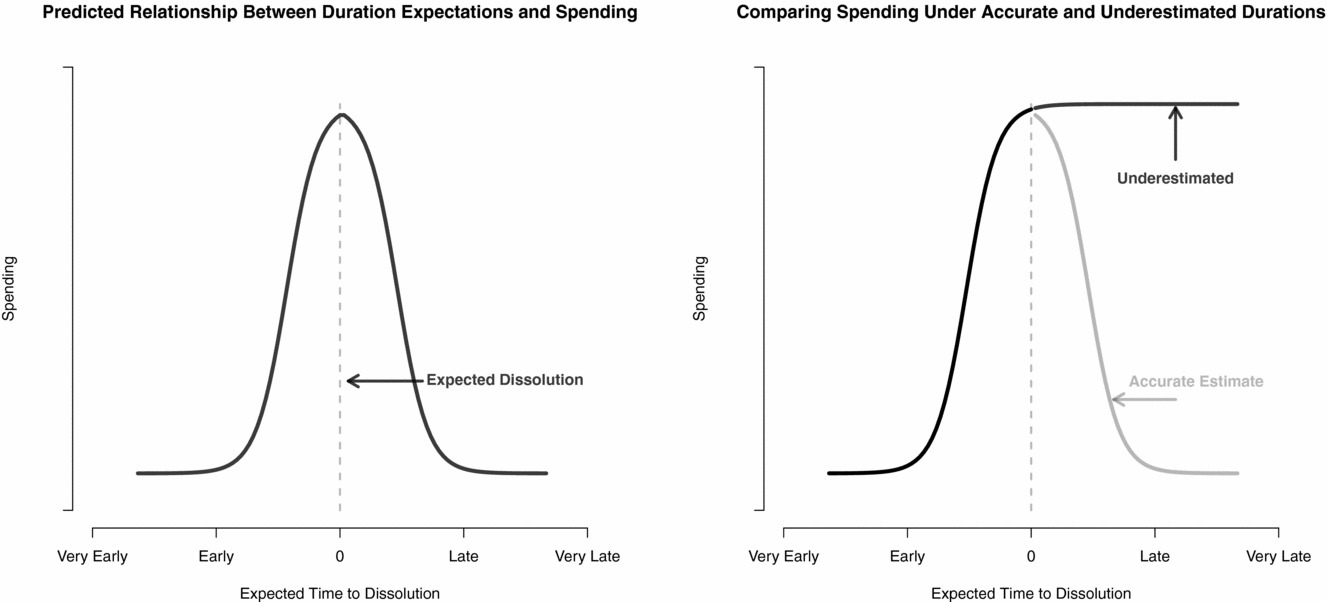
Borrowing from Alt and Lassen (Reference Alt and Lassen2006), a stylized representation of this expectation is given in the left pane of Figure 1 with the x-axis representing the cabinet’s life expectancy and the y-axis representing public spending. As the government’s expected dissolution point approaches (indicated by the 0 hash on the x-axis), it increases spending to engender electoral support. After the election, the government (whether or not the incumbent has returned) lowers spending and the cycle begins again. To reiterate: when governments believe that elections are distant, public spending is more modest. When governments believe that elections are approaching, however, they begin to spend more boldly in an effort to stimulate electoral support. This is the central hypothesis that we test below.Footnote ¹¹

FIGURE 1.

Duration Expectations and Public Spending

Thinking of dissolutions as stochastic and public spending as a function of forecasted durations raises a follow-up question: What happens when the cabinet’s prediction is wrong—either too generous or too miserly—by some significant margin? To the former, when a cabinet forecasts a duration that is too long and terminates earlier than expected, it should lose votes. In this case, the premature termination would preclude the government from ramping up spending to stimulate support and, as a result, its electoral performance should suffer. This prediction is supported by the extant literature on electoral timing and success. For example, Smith (Reference Smith2003) presents compelling evidence that incumbents perform more poorly than expected in early elections.Footnote ¹²

To the latter, when the cabinet forecasts a duration that is too short and terminates later than expected, there is no impact on the electoral result, but there should be an increase in the government’s propensity to run deficits. A stylized depiction of this expectation is given in the right pane of Figure 1. When the cabinet’s prediction of its duration is accurate, we should observe an increase in spending, an election, and then a decrease in spending about the 0 point on the x-axis. This is shown by the lighter line. The darker line, on the other hand, shows the expectation for an underestimate of the cabinet’s durability. In this case, the government increases spending in expectation of elections, but, when the cabinet proves more durable than anticipated, it must continue to spend at the heightened rate until dissolution to maintain its electoral support. The longer these protracted periods of heightened spending exceed the cabinet’s expectations, the deeper they will push the state into deficit. This is the second hypothesis we test—the longer a cabinet outlives its expected duration, the greater its deficit spending.

Before moving on to our design, it is important to note that cabinet dissolutions are not entirely stochastic—cabinets must terminate at the end of the CIEP and may choose to terminate for strategic reasons (given that the institutional context allows) at any time. The first issue is easily accounted for and we explain that below. The second issue requires a bit more contemplation. Recalling Kayser (Reference Kayser2005), cabinets may choose to influence potential electoral results by increasing spending (our focus here) or calling for early elections, or they may choose to remain in office without engaging in opportunistic behaviors and this choice is conditioned on exogenous economic shocks and the time remaining in the CIEP.Footnote ¹³ This presents potential hurdles, both systematic and stochastic in nature, that warrant discussion before moving on.

One possibility is that governments increase spending to stimulate popularity and call for opportunistic elections once estimated support reaches some critical level. Under this condition, we may observe a negative relationship between expected duration and public spending, just as we predict, albeit due to an alternative (though very closely related) mechanism, because expected durations are correlated with true durations. For lack of more clever language, we can call this budget cycling under complete electoral endogeneity, as opposed to budget cycling under duration uncertainty—a systematic behavior that may confound our ability to assess our arguments. Fortunately, theses mechanisms are empirically differentiable with the data on hand. If, as we argue, governments form expectations of their durability and plan their spending accordingly, then expected durations should provide more predictive power for observed rates of spending. On the other hand, if elections are, on average, chosen opportunistically after governments have increased spending, then true durations should provide more predictive power for observed rates of spending, because, in this case, spending and electoral timing are codetermined. To preview our empirical results, spending patterns are better explained by expected durations. We also add that, if cycling under electoral endogeneity was the norm, then past PBC research would not have failed to recover evidence of cycling behavior in these countries as often as it has.

A second possibility is that cabinets privileged by some exogenous shock creating a windfall of popularity may call early elections without having to ramp up spending in the manner we predict—a stochastic occurrence that may confound assessment of our theoretical argument. Of course, this second possibility would not produce our predicted relationship, rather, this type of opportunistic behavior would bias against recovering support for our hypothesis. And, because our focus is the effect of cabinet durability on public spending, rather than the relationship among economic inputs (e.g., spending, inflation), economic outputs (e.g., growth, unemployment), and electoral timing and performance, opportunistic elections of this type are stochastic nuisances rather than threats to design credibility. We also note that if the true process guiding spending patterns is some combination of systematic cycling under electoral endogeneity and stochastic opportunism, then, again, true durations would provide a better fit to our spending data vis-à-vis expected durations. We return to this issue and other potential confounders in a short section on robustness following our empirical analysis.

RESEARCH DESIGN

To test our hypotheses, we first develop a model of duration expectations for the cabinet. We assume that cabinets take into account the observable characteristics of their government and accordingly generate their expectations for its duration, with greater or lesser degrees of certainty. That is, because governments cannot reasonably be expected to foresee the precise timing of “critical events” such as economic downturns, political scandals, or abrupt fluctuations in public opinion, the best information they have to generate their expectations are the life cycles of governments past, the observable characteristics of those governments, and the attributes of their own cabinet—a form of Muth’s (Reference Muth1961) classic rational expectations.Footnote ¹⁴

The most obvious starting point for estimating these expectations is the rich political science literature on the durability of governments discussed above. After the work of, for example, King et al. (Reference King, Alt, Burns and Laver1990), Laver and Shepsle (Reference Laver and Shepsle1998), Diermeier and Stevenson (Reference Diermeier and Stevenson2000), and Chiba, Martin, and Stevenson (Reference Chiba, Martin and Stevenson2015), there can be little doubt that political scientists have amassed an impressive understanding of the theoretical foundations and empirical correlates of cabinet stability. Thus, to generate our measure of a government’s life expectancy, which we will impute to the cabinet, we accept the collective wisdom of the discipline and derive our measure from the extant literature. More specifically, we estimate the survival model described in Chiba, Martin, and Stevenson (Reference Chiba, Martin and Stevenson2015), which accounts for potential selection bias induced by strategic formations by jointly modeling formation and duration. Note that, as King et al. (Reference King, Alt, Burns and Laver1990) explain, this duration model captures “events” in its stochastic component (distributed Weibull in this case), while including “attributes” as the measured covariates in its systematic component. For all cabinets in our data, we use the model estimates to predict the number of days the cabinet will last before dissolution.

Importantly, we do not pool the risks of dissolution and replacement.Footnote ¹⁵ We make this choice for two reasons. First, the risk type that is theoretically salient is dissolution and, as such, we do not want replacement terminations contributing to our durability estimates. Second, cabinets have no incentive to prepare for replacement rather than dissolution. In the event of a replacement, the incumbent loses its governing status and is consigned to opposition. Given what we have learned about the collective memory of voters, when the next election arrives, it is not the displaced incumbent that is the focus of competency evaluations, but its successor and any choices made by the displaced incumbent are likely to be irrelevant (or nearly so) to the election outcome (Healy and Lenz Reference Healy and Lenz2014).Footnote ¹⁶ Taken together, these factors imply that a cabinet’s best strategy would be to ignore replacement risk when generating its expectations for durability. Fortunately, the data allow us to bring evidence to bear on the question of expectation formation under competing risks and we discuss this in the robustness section.

Our public spending analysis is conducted at the country-year level. Therefore, to capture each cabinet’s expected remaining time in office when the budget is set, we subtract from the cabinet’s total predicted life the number of days the cabinet has already served at the time it presents its annual budget to the legislature. This estimate of the cabinet’s remaining life expectancy is the covariate of interest in our models of public spending (explained in detail below). We expect this to have a negative relationship to public spending in general—that a cabinet will spend more as its expected duration dwindles—and a negative relationship to deficit spending—that a cabinet will spend less responsibly as its expected duration dwindles. Of course, our measure of the cabinet’s duration expectations is estimated with error, and, as such, we take care to model this error structure.

Data and Model Construction

For our main analyses, we gather data on several decades of budgeting in 15 European democracies that allow for parliamentary dissolutions—the same data analyzed by Bawn and Rosenbluth (Reference Bawn and Rosenbluth2006) and Martin and Vanberg (Reference Martin and Vanberg2013).Footnote ¹⁷ Our dependent variables are the OECD calendar-year estimates of central government spending as a percentage of GDP and this spending figure minus central government receipts as a percentage of GDP, where greater values indicate greater deficits. Budgets in our sample are typically submitted in the latter half of the year for spending in the following calendar year. Most submission dates fall between August and October of the calendar year preceding the budget year, though dates as early as July and as late as April of the budget year appear in the data.Footnote ¹⁸ The data also include information on several political economic characteristics salient to budget-making, which we discuss below.

The explanatory variable of interest is the cabinet’s predicted duration—the number of days it expects to remain in office—at the time the budget was submitted. We derive the measure by first reestimating Chiba, Martin, and Stevenson’s (Reference Chiba, Martin and Stevenson2015) model of government duration, which jointly estimates cabinet formation and survival.Footnote ¹⁹ To account for uncertainty in this estimate, we employ a nonparametric bootstrap.Footnote ²⁰ At each of the 1,000 bootstrap iterations, we randomly resample the data, with replacement, from our set of 432 cabinets and reestimate the model. We then use the model estimates to predict the duration for each cabinet in our data, record the predictions, and reiterate, generating a distribution of 1,000 predicted survival times for each cabinet.

For each cabinet-budget year in our spending data, we alter these distributions in two ways: (1) we subtract the number of days the cabinet has served at the time of budget submission and (2) we trim any expected durations that exceed the CIEP back to the expiration of the CIEP. Predicted durations exceeding the CIEP are fairly rare, but must nonetheless be accounted for—no government can reasonably expect to remain in office through the CIEP without holding elections.Footnote ²¹

By estimating a distribution of expected durations for each of our sample cabinets, we have a straightforward way of accounting for the uncertainty of these predictions. This is important for both empirical and theoretical reasons. Empirically, this variable is, after all, an estimate with an associated error structure and ignoring this error may bias our estimates of the relationships of interest, and therefore bias our substantive conclusions. Theoretically, expectations rarely take the form of a point when they are generated by individuals and are explicitly distributions when they are generated by a collective, whether it is a system of firms, a betting market, or the ministers composing a cabinet. If we assume that rational expectations are distributions that are, in the aggregate, centered on the most probable (or, most expected, given the state of the world) outcome as Muth (Reference Muth1961) theorized and others have found empirically, then modeling these distributions, rather than merely their central tendency, is critical to hypothesis testing.

We model these distributions by estimating our spending and deficit models 1,000 times—once for each prediction of cabinet survival. Thus, for each iteration, we impute an expected remaining duration for each cabinet-year in our data using a single set of bootstrapped survival predictions, estimate the spending and deficit models, and record the results. This yields 1,000 regression results for the main models which we summarize and interpret below, but we first discuss the construction and estimation of the spending models.

Alongside our focal variable (predicted duration), we include a set of political economic control variables borrowed from Bawn and Rosenbluth (Reference Bawn and Rosenbluth2006) and Martin and Vanberg (Reference Martin and Vanberg2013) to account for potential confounders to our relationship of interest while keeping our substantive results comparable to previous research. The measurement of these covariates and the reasons they are included in the models are described in great detail by Bawn and Rosenbluth and Martin and Vanberg, so we do not reiterate that information here. We provide, instead, a more general discussion of the rationale motivating inclusion of these covariates which break down into three groups: variables capturing the government’s taste for public spending; variables accounting for the state’s revenue supply and entitlement burden; and variables indicating institutional constraints on spending depth and responsibility.

First, consider spending tastes, or the breadth of spending demands within the cabinet. There is broad theoretical consensus in the literature is that left-leaning parties prefer to spend more than right-leaning partiesFootnote ²² and we account for this by including Powell’s (Reference Powell2000) measure of the cabinet’s ideological positioning: the mean, seat-weighted, left-right stance of each member of the cabinet, where greater values indicate a more right-leaning government.Footnote ²³ Following the above discussion on the common pool resource problem in budgeting—as the diversity of spending priorities grows, the cabinet’s temptation to spend to please its supporters increases—we include the number of parties in the cabinet. We also include the effective number of legislative parties (Laakso and Taagepera Reference Laakso and Taagepera1979) to account for the possibility that diverse spending priorities outside the cabinet may coax budgets upward in a similar fashion.

Our second set of controls are meant to account for a state’s ability or need to grow its spending obligations. That is, does the state in question have the resources needed to increase spending responsibly, or, are there characteristics of the state that should systematically increase its spending obligations? These variables include: the overall level of economic productivity (measured as per capita GDP), a state’s integration into the modern trade economy (called “trade openness” in the tables below; the export/import fraction of GDP), its unemployment rate, and the percentage of likely nonproductive population—those under 15 years of age and those 65 and over (called the “dependency ratio”).

Finally, we include two variables meant to capture domestic and supranational spending constraints. The first is Martin and Vanberg’s (Reference Martin and Vanberg2013) “budgetary constraint index,” a summary of formal rules that “[c]onstrain the ability of parties to push for spending,” and, “generate incentives for parties to oppose spending demands by their partners” (p. 956). This variable is bounded between 0 and 1 and is interacted with the number of parties in the cabinet. The second is a binary variable indicating that the budget was submitted after the adoption of the Maastricht Treaty, which placed limits on the total debt a member state could carry, as well as the size of the deficit a state could generate in any given year. Interested readers may see summary statistics for all variables in the appendix.

With variables in hand, we now turn to estimation. We are analyzing panel data with substantial cross-sectional variation, but also a great deal of autocorrelation within units. Following Bawn and Rosenbluth (Reference Bawn and Rosenbluth2006) and Martin and Vanberg (Reference Martin and Vanberg2013) we estimate an autoregressive distributed lag model (ADL), including (one year) lags of both the dependent variables and independent variables as well as concurrent realizations of the economic variables and estimate panel-corrected standard errors. This is in keeping with Philips’s (Reference Philips2016) conclusion that modeling data dynamics is vital in the analysis of public spending, as ignoring the autoregressive properties of spending patterns can lead to inflated estimates of cycling behavior.Footnote ²⁴ As our focal explanatory variable is a distribution, rather than a point, we cycle through its 1,000 estimated values, imputing each into our spending and deficit models in turn, estimating, and recording the results. We also generate error estimates on our cabinet ideology measure following Lowe et al. (Reference Lowe, Benoit, Mikhaylov and Laver2011) and model these in the same fashion.

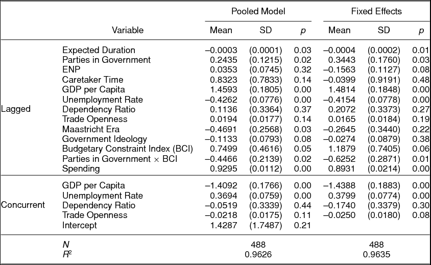
The results of our first model, public spending, are summarized in Table 1.Footnote ²⁵ For our covariate of interest, expected duration, there is a statistically significant negative parameter estimate, indicating, as we predicted, that decreasing expected duration will increase the cabinet’s level of public spending. Further, each of our control variables, when reaching statistical significance, are signed in the sensible direction and comport with previous research on spending (e.g., Bawn and Rosenbluth Reference Bawn and Rosenbluth2006; Martin and Vanberg Reference Martin and Vanberg2013), giving us confidence that our model is properly specified.

TABLE 1.

Aggregated Results from Bootstrapped Model of Spending as Percent of GDP

p = directional certainty, fixed effects not shown

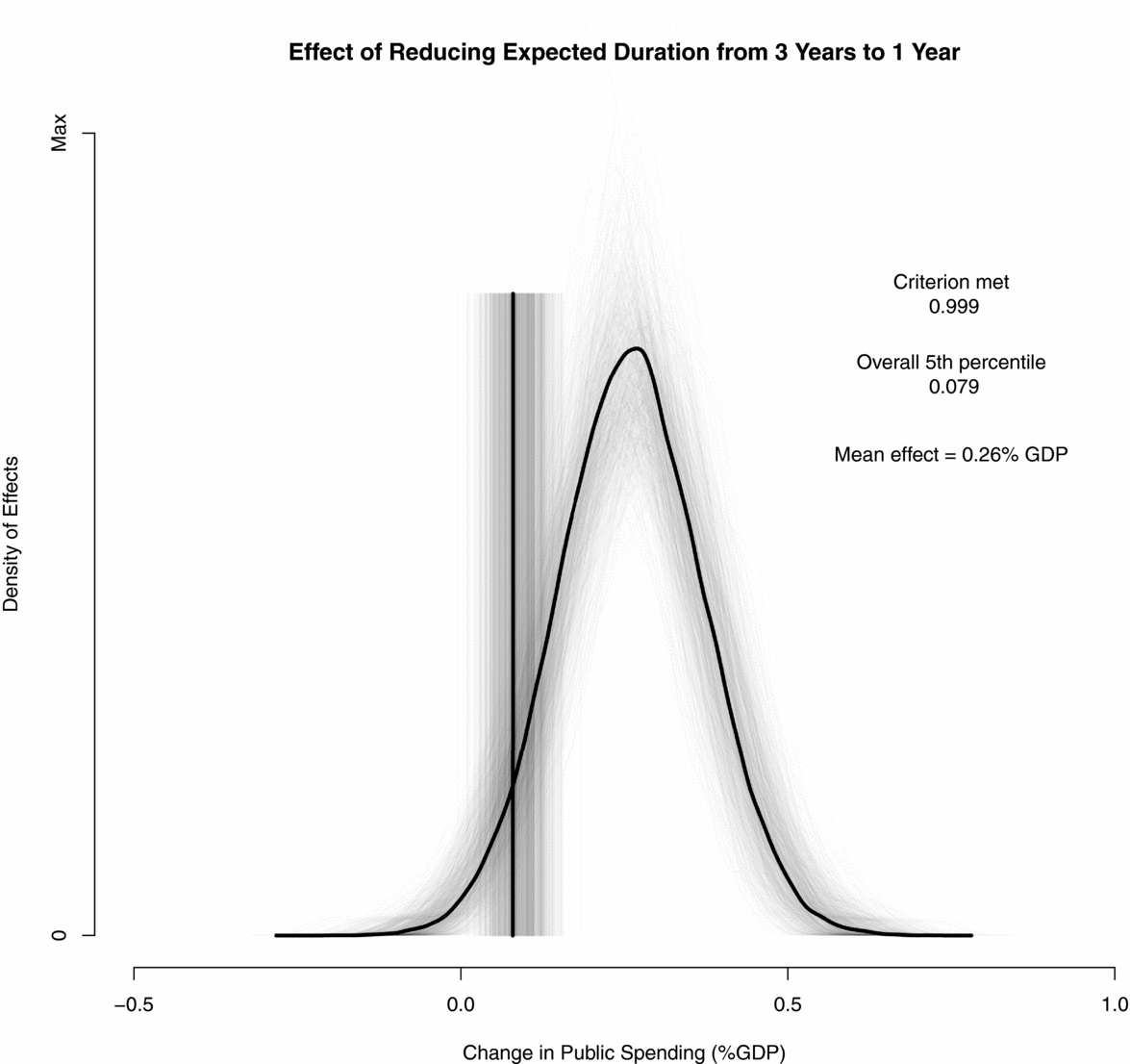
To better illustrate the predicted effect of expected duration on public spending, Figure 2 plots the substantive effect of a reduction in expected cabinet duration from three years to one year, aggregated across all of our 1,000 models. Each light density in Figure 2 plots the distribution of predicted changes in spending as a percentage of GDP resulting from this reduction in the expected durability of the cabinet from a single bootstrap iteration. Thus, the shape of each light density illustrates the estimation uncertainty in one of our 1,000 models and the light vertical lines mark the fifth percentile of each distribution (our criterion for statistical significance). The thicker, darker lines give the global density and fifth percentile over all bootstrap iterations. Taken together, the figure shows that, not only is our criterion for statistical significance met in virtually all bootstrapped models, but also that there is very little variation in this result across the 1,000 bootstrapped models.

FIGURE 2.

The Effect of Expected Duration on Spending

More substantively, on average, the decrease from three years to one year of expected duration (about a 1.5 standard deviation change) increases public spending by 0.26% of GDP. This is a very large spending increase. Using 2010 GDP and spending figures in US dollars, we can get a better sense of how salient this effect is: for Denmark (GDP $320 billion) the increase would be roughly $844 million, for the Netherlands (GDP $836 billion) the increase would be over $2.2 billion, and for Germany in the same year (GDP $3.4 trillion) the increase would be just shy of $9 billion. To contextualize these figures, this increase equates to roughly 11.5%, 16.5%, and 17.6% of the unemployment cash transfers made in these countries, or 18.9%, 19.7%, and 19.5% of defense spending in these countries, respectively. These effects are quite large and we are quite certain of them, indeed, only 1 in 1,000 models yields a certainty estimate that does not meet the p < 0.05 criterion and fewer than 1% of all posterior draws are greater than 0. This is very strong support for our first hypothesis: cabinets spend more as their expected time in office dwindles.

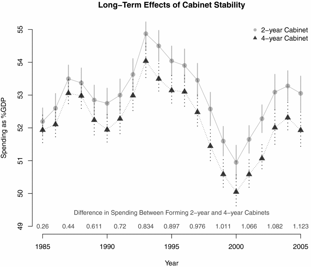
Of course, the effects of durability should be larger and much longer lasting than this one-time increase, however. Budgets tend to be remarkably sticky. As such, small increases made here and there have a tendency of becoming effectively permanent. Following Williams and Whitten (Reference Williams and Whitten2012), we illustrate the compounding nature of cabinet fragility in Figure 3 where we plot the public spending of Austria under two idealized scenarios: one in which Austria always forms four-year cabinets (dark triangles) and one in which it always forms two-year cabinets (light circles). To generate the values, we use the parameter estimates summarized in Table 1 to predict Austrian spending levels from 1985 to 2005, using its observed covariate values over that period, with the exception of expected durability and lagged spending. For one case, we count down expected duration from four years to one year and repeat; for the second case, we count down from two years to one year and repeat. Also, for each year (after the first) we use the mean of the previous year’s predicted spending as the lagged spending value. As the figure shows, persistent cabinet instability of this magnitude can substantially increase spending over the long term.

FIGURE 3.

The Compounding Effects of Duration on Spending

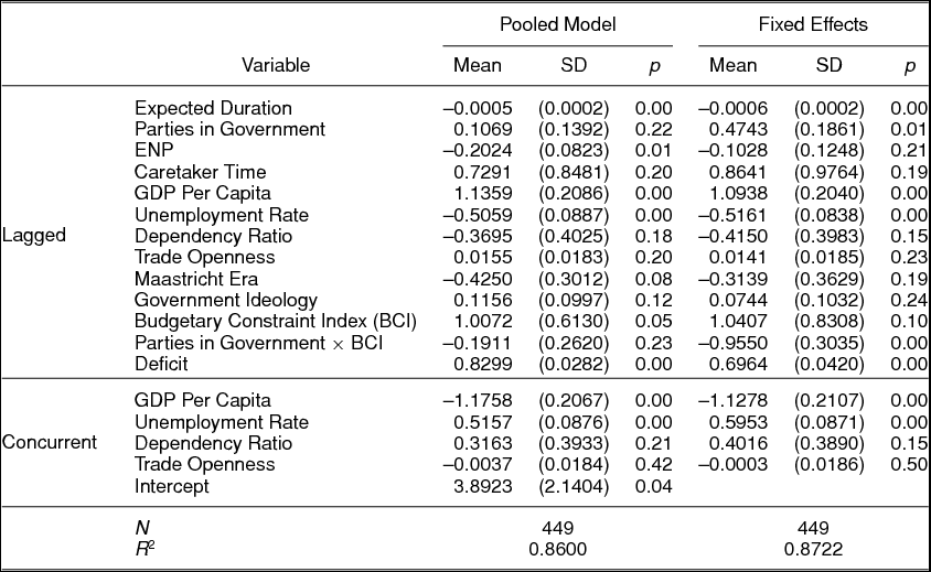
We now move on to our deficit models, which are estimated and presented in the same fashion as above in Table 2. As with our spending model, our covariate of interest, expected cabinet duration, is negative and clearly different from zero, indicating that as the cabinet’s expected time in office draws to a close it begins to spend less responsibly—i.e., running ever-higher deficits. Further, as before, the control variables with robust estimates are all signed in the direction that we would expect, making us confident in the model specification. We also note here that there are really three ways to estimate this model: using only the expected remaining duration, folding that expected duration into a binary variable, indicating that the cabinet has outlived its expectations (duration < 0), or estimating an implied interaction of the duration measure and the indicator. We present the results of the first method in the main text to match the previous analysis, however all three produce very similar results and the remaining two models are given in the Appendix.

TABLE 2.

Aggregated Results from Bootstrapped Model of Spending Deficits as Percent of GDP

p = directional certainty, fixed effects not shown

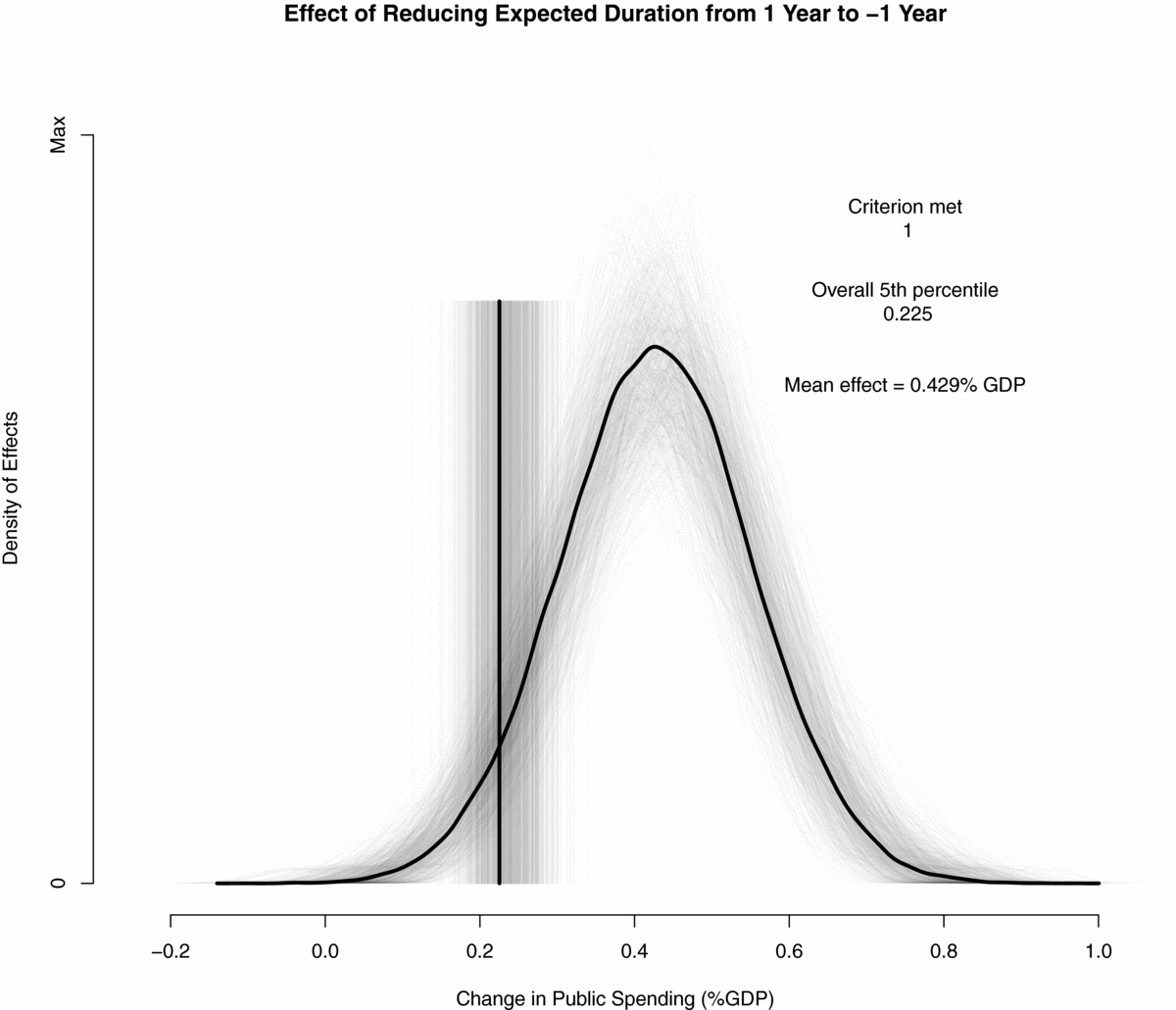
As predicted, expected duration is negative and the estimate is strongly significant (p < 0.01). As above, we interpret these results graphically by predicting the change in deficit size as a function of a change in expected cabinet duration (using the fixed effects model results, once again). The difference here is that we change expected duration from one year to –1 year, indicating that the government has outlasted its life expectancy by a year (there are several such cases in our sample). These results are given in Figure 4, where the densities illustrate the entire distribution of predicted deficit changes and the vertical lines illustrate the fifth percentile of each distribution. First, the effects, as before, are very large. The change from an expected one year of remaining time in office to outliving expectations by one year results in an average 0.422% increase to the deficit. This is a substantial and normatively significant increase, not only because increases to the present deficit are so large, but also because the true long term cost of this deficit increase is compounded by the interest payments made over the debt clearing window. Notice also that we are extremely confident in the direction of the effect—each model yields an estimated certainty of p < 0.05.

FIGURE 4.

The Effect of Expected Duration on Deficit Spending

It is worth taking a moment to consider how this finding informs our understanding of how incumbents value their current time in office as opposed to their electoral prospects. Our theoretical arguments and empirical evidence suggest that cabinets forecast their durability, plan their spending to crescendo as forecasted dissolution approaches, and, if they prove more durable than expected, continue to spend lavishly to maintain support until dissolution. This suggests that incumbents prefer to continue to serve their present term, running the country ever higher into deficit, than to call early elections. At the least, this evidence suggests that, on average, incumbents are more averse to the uncertainty of elections than they are to incurring the wrath of voters for irresponsible spending. A broader interpretation of this finding is that incumbents are more averse to electoral uncertainty than most current characterizations of the literature may imply—that we have perhaps been too cavalier in our assumptions of an incumbent’s willingness to call for new elections. Of course, there is good reason for this. Though some dissolution models had built in electoral uncertainty (e.g., Kayser Reference Kayser2005), a simplifying assumption of many more formal models of dissolution is that the outcome of the election is common knowledge across all parties (e.g., Diermeier and Stevenson Reference Diermeier and Stevenson2000).

ROBUSTNESS

The models presented above reveal strong support for our central predictions, but there are a few issues that we wish to address before concluding. First, the manner in which expected duration enters the model makes, for example, a cabinet with a two-year expected duration in its first year in office equivalent to a cabinet with a four-year expected duration in its third year in office. It is therefore possible that the effects reported above may not be driven by expiring expected durations, but instead by shorter total expected duration, which may stimulate a need to spend more rapidly for the government to achieve its desired policy outcomes within its abbreviated life expectancy. We assess this possibility in the Appendix, where we include in our models both the cabinet’s remaining life expectancy and its entire life expectancy. In these models, the remaining life expectancy remains negative and robust while there is no statistically differentiable effect for total life expectancy.

A second possibility is that cabinets are making their spending choices not according to expectations as we conceive of them, but according to the CIEP, assuming, or hoping, the cabinet will last the entirety of its potential duration. This, too, may produce the effects that we uncover above as predicted durations and CIEP are positively correlated. We assess this possibility by including both our measure of expected duration and the maximum possible duration (time left in CIEP) in the model. Again, our substantive results remain, while CIEP has no statistically discernible relationship to spending.

Third, previous readers have suggested that we may introduce bias into our estimates by neglecting to model a cabinet’s ability to call early elections. As we discussed above, strategically timed elections following a stochastic windfall in popularity should only induce bias against finding our predicted effect. On the other hand, elections strategically timed to coincide with a planned increase in spending may potentially produce empirical results similar to what we have uncovered. While this is still electoral manipulation and budget cycling, this is not the theoretical story we are telling and we wish to reassure readers that these processes are not driving our results. We do this in two ways.

As mentioned earlier, if cycling under completely endogenous elections is a more accurate description of spending decisions, then true government durations would provide a better fit to the data than expectations as these durations and spending levels are codetermined. To test this, we reestimate our models after replacing our key measure with true durations and then reestimate again with both measures included. In both models, true durations do not provide statistically significant explanatory power and when both values are included the estimate on expected durations is still large, negative, and statistically robust.

Our second approach is to simultaneously estimate the cabinet’s choice of opportunistic election—using Schleiter and Tavits’ (Reference Schleiter and Tavits2016) data on opportunistic elections, which cover our entire sample—and the cabinet’s total public spending and deficit spending, given its early election choice. We do this by instrumenting opportunistic elections with Goplerud and Schleiter’s (Reference Goplerud and Schleiter2016) index of the assembly dissolution powers vested in the cabinet—a variable that should only affect spending through its impact on early elections. Our substantive results remain in this framework as well.

A fourth concern was noted in our research design section, where we discussed how cabinets should approach competing risks to termination and concluded that they should ignore the potential for replacement because there is simply no expected benefit to anticipating replacement. Our data allow us to get some traction on this question by estimating termination as a function of dissolution (as we did for the models above), replacement, and pooled risk, imputing predicted durations from these different survival models into our spending models, and comparing model fit. As our arguments imply, durations derived from models of dissolution risk perform better than pooled risk predictions, and pooled risk predictions perform better than replacement predictions. Because they are quite highly correlated, all measures produce statistically significant estimates of the predicted effect, but the rank-ordering of empirical fit follows a theoretical rank-ordering where cabinets are concerned with dissolution, but have less (or no) incentive to anticipate replacement.

A final potential concern is our choice of dependent variable as previous research has noted that cycles may be more evident in the composition of spending than in the level of spending and analyzing the level of spending alone may obscure the overall effect of cycling behavior. We have estimated replications of the total spending analysis that only examine social spending (unemployment benefits, pensions, housing transfers, etc.) and these models produce results that are similar in magnitude and a shade more powerful than our total spending models. There are good reasons to focus exclusively on social spending—most importantly, one could argue that this would be the most direct way to stimulate electoral support as these are largely redistributive transfers. However, we contend that total spending is the more appropriate subject of study here because spending is not just a tool of economic stimulus in our theoretical argument, but also a means of satisfying the priorities of core supporters.

SUPPLEMENTARY MATERIAL

To view supplementary material for this article, please visit https://doi.org/10.1017/S0003055418000436.

Replication materials can be found on Dataverse at: https://doi.org/10.7910/DVN/HHMXU3.