1 Introduction
Two-phase flow processes involving transport of solid particles through gas are of central importance to pharmaceutical, food product, chemical and energy industries. A theory that is capable of accurately predicting the complicated behaviour involved in such processes is therefore crucial and of significant practical value. The dynamics of particulate flows, either granular (negligible interstitial fluid) or multiphase, is extraordinarily complex as even the simplest gas–solid flows are known to exhibit instabilities that manifest as persistent, transient and inhomogeneous solids distributions commonly referred to as clustering (Goldhirsch Reference Goldhirsch2003; Fullmer & Hrenya Reference Fullmer and Hrenya2017b ) or bubbling (Jackson Reference Jackson2000; Sundaresan Reference Sundaresan2003) depending on the solids concentrations. The distinction, however, is largely cosmetic, as the mechanisms underlying bubbling and clustering instabilities are the same (Glasser, Sundaresan & Kevrekidis Reference Glasser, Sundaresan and Kevrekidis1998).
Like turbulence in molecular fluids, clustering in rapid granular and gas–solid flows is more the rule than the exception. Owing to the pervasiveness of clustering, numerical methods used to model particulate flows need to accurately describe this instability owing to its large impact on interfacial coupling. One of the available methods is the discrete element method (DEM), which tracks the motion of every particle. DEM (sometimes referred to as molecular dynamics, MD) studies provided some of the earliest reported evidences for clustering in granular systems (Hopkins & Louge Reference Hopkins and Louge1991; Goldhirsch & Zanetti Reference Goldhirsch and Zanetti1993). DEM may also be coupled with a computational fluid dynamics (CFD) solver for multiphase simulations. If a volume-averaged approach is used, in which the fluid grid size is typically larger than the particle size, the coupled method is frequently referred to as CFD-DEM. CFD-DEM has become a reliable method for the simulation of fluid–particle flows and has been used to study clustering and bubbling instabilities in, for example, fully periodic sedimentation (Radl & Sundaresan Reference Radl and Sundaresan2014; Capecelatro, Desjardins & Fox Reference Capecelatro, Desjardins and Fox2015), wall bounded fluidization (Tsuji, Tanaka & Yonemura Reference Tsuji, Tanaka and Yonemura1994; Vreman et al. Reference Vreman, Geurts, Deen, Kuipers and Kuerten2009; Capecelatro, Pepiot & Desjardins Reference Capecelatro, Pepiot and Desjardins2014) and bubbling in dense fluidized beds (Tsuji, Kawaguchi & Tanaka Reference Tsuji, Kawaguchi and Tanaka1993; Ye, van der Hoef & Kuipers Reference Ye, van der Hoef and Kuipers2005; Hou, Zhou & Yu Reference Hou, Zhou and Yu2012; LaMarche et al. Reference LaMarche, Liu, Kellogg, Weimer and Hrenya2015), among others. If a very fine fluid grid is considered, approximately an order of magnitude smaller than the particles, direct numerical simulations (DNS-DEM or simply DNS) may be performed in which all relevant scales of motion of both phases are explicitly resolved (Tenneti & Subramaniam Reference Tenneti and Subramaniam2014). Although less pervasive than CFD-DEM due to its high computational overhead, DNS has been used to study clustering in a homogeneous cooling system (HCS) (Wylie & Koch Reference Wylie and Koch2000; Yin et al. Reference Yin, Zenk, Mitrano and Hrenya2013; Garzó et al. Reference Garzó, Fullmer, Hrenya and Yin2016) and fully periodic sedimentation/fluidization (Kajishima & Takiguchi Reference Kajishima and Takiguchi2002; Derksen & Sundaresan Reference Derksen and Sundaresan2007; Wang et al. Reference Wang, Zhou, Wang, Xiong and Ge2010b ; Uhlmann & Doychev Reference Uhlmann and Doychev2014; Rubinstein, Derksen & Sundaresan Reference Rubinstein, Derksen and Sundaresan2016; Liu, Wang & Ge Reference Liu, Wang and Ge2017).
Although increased access to supercomputers and their ever-expanding capability has allowed for DNS and CFD-DEM simulations with impressive particle counts – several groups have simulated over 10 million particles via CFD-DEM (Capecelatro & Desjardins Reference Capecelatro and Desjardins2013; Capecelatro et al. Reference Capecelatro, Desjardins and Fox2015; Morris et al. Reference Morris, Ma, Pannala and Hrenya2016) – the current capabilities of discrete particle simulations still fall well short of industrial and engineering needs, for which systems may contain trillions of particles. Presently, methods that treat the particles as a continuum are most commonly used for the simulation of large systems. In the absence of an interstitial fluid, continuum models for granular flows are typically derived using kinetic theory (KT) approaches (Lun et al. Reference Lun, Savage, Jeffrey and Chepurniy1984; Garzó & Dufty Reference Garzó and Dufty1999; Brilliantov & Pöschel Reference Brilliantov and Pöschel2004). In the case of two-phase flows, i.e. solids with an interstitial fluid present, the two-fluid model (TFM) treats the phases as interpenetrating media. If the particles are ‘moderately massive’, the closure relations and transport coefficients typically used for granular flows may be directly amenable to the solids phase of the TFM for gas–particle flows (Sinclair & Jackson Reference Sinclair and Jackson1989; Gidaspow Reference Gidaspow1994; Lun & Savage Reference Lun and Savage2003). Recently, more accurate approaches for multiphase flows have been undertaken which consider fluid-phase effects at the starting point, i.e. in the Enskog kinetic equation (Koch Reference Koch1990; Gidaspow Reference Gidaspow1994; Koch & Sangani Reference Koch and Sangani1999), also see Garzó et al. (Reference Garzó, Tenneti, Subramaniam and Hrenya2012) and references therein. The acronym KT-TFM is used here instead of the more common KTGF (kinetic theory of granular flow) to distinguish the resulting multiphase model from single-phase (granular) continuum models, e.g. Garzó & Dufty (Reference Garzó and Dufty1999).
Even with empirical (rather than KT-based) closures, the TFM has been known to predict the clustering instability in gas–solid multiphase flows – at least qualitatively – since the late 1980s (Gidaspow, Tsuo & Luo Reference Gidaspow, Tsuo and Luo1989; Tsuo & Gidaspow Reference Tsuo and Gidaspow1990). A little over a decade later, Agrawal et al. (Reference Agrawal, Loezos, Syamlal and Sundaresan2001) demonstrated that the properties of clustering in continuum predictions were highly dependent on the numerical grid and reported that a resolution on the order of ten particle diameters was necessary for the slip velocity and granular temperature to become grid insensitive. In intermediate and dense flows, the grid requirement is even more demanding to resolve the sharp gradients at the cluster or bubble interface (Wang, van der Hoef & Kuipers Reference Wang, van der Hoef and Kuipers2009; Fullmer & Hrenya Reference Fullmer and Hrenya2016). Such a high level of resolution likewise precludes high-resolution KT-TFM from being used to simulate industrial-scale systems. One of the most promising approaches used to simulate large systems are filtered TFMs, see, for example, (Igci et al. Reference Igci, Andrews, Sundaresan, Pannala and O’Brien2008; Wang, van der Hoef & Kuipers Reference Wang, van der Hoef and Kuipers2010a ; Parmentier, Simonin & Delsart Reference Parmentier, Simonin and Delsart2012; Schneiderbauer & Pirker Reference Schneiderbauer and Pirker2014) and follow-on works. Similar to large eddy simulation (LES) of turbulent single-phase flows, filtered TFMs aim to only resolve the large scales of motion and model the effect of subgrid-scale structures. However, the subgrid-scale models in filtered TFMs are considerably more complicated than for single-phase turbulent flows due to interfacial transfer (Fox Reference Fox2012) and high-resolution KT-TFM simulations are frequently used to constitute many of the subgrid-scale closures (Igci & Sundaresan Reference Igci and Sundaresan2011; Ozel, Fede & Simonin Reference Ozel, Fede and Simonin2013).
While KT-TFMs now seem to be generally accepted as a valid approach for gas–solid flows (Fox Reference Fox2014), the quantitative accuracy of such models remain largely unknown, particularly for systems that display clustering instabilities. In particular, such instabilities are characterized by a large concentration gradient across the cluster interface, which likely violates the low Knudsen number assumption inherent in the derivation, as was previously found for granular flows (Mitrano et al. Reference Mitrano, Zenk, Benyahia, Galvin, Dahl and Hrenya2014). Some attempts have been made to compare high-resolution KT-TFM results directly to experimental data (Wang Reference Wang2008; Benyahia Reference Benyahia2012; Cloete, Johansen & Amini Reference Cloete, Johansen and Amini2012), although such comparisons usually require simplifying the geometry or dimensionality of the system. Furthermore, experimental data may contain effects due to additional physics not considered by the KT-TFM, e.g. aspherical, polydisperse particles, surface roughness, relative humidity in a gas, van der Waals forces, electrostatics, etc. While prediction of physically realistic conditions is the ultimate goal, comparison to experimental data may not be the most appropriate first step in validating KT-TFMs because it is non-trivial to determine a posteriori if discrepancies between simulation and experimental data are associated with assumptions of the experimental system (e.g. particle and fluid properties) or assumptions inherent to the continuum derivation. Due to the large number of assumptions required by most KT-TFMs, e.g. see §§ 2.1.1–2.1.3, a two-pronged approach to validation is desirable, comparing first to ideal numerical data and then to realistic experimental data. Discrete particle simulations such as dissipative MD, CFD-DEM, and DNS offer ideal validation data as all or most of the assumptions of the KT-TFM are upheld except those that are required in the discrete-to-continuum derivation. KT-based continuum models for granular flows have been validated in the HCS for the onset of the velocity vortex instability (Mitrano et al. Reference Mitrano, Garzo, Hilger, Ewasko and Hrenya2012) and the clustering instability (Mitrano et al. Reference Mitrano, Zenk, Benyahia, Galvin, Dahl and Hrenya2014) by comparing to MD data. Similarly, for gas–solid flows, the onset of velocity vortices in the HCS was also recently analysed by comparing predictions from a linear stability analysis of the KT-TFM to DNS data (Garzó et al. Reference Garzó, Fullmer, Hrenya and Yin2016). The agreement between the continuum and discrete particle data in the gas–solid case was acceptable, but noticeably deteriorated compared to the granular case. (We note that this deterioration may trace to differences in the linear stability analysis rather than the KT-TFM theory itself.) While the HCS serves as a good first test, it has only been used to analyse the onset of instabilities when the system is only weakly nonlinear. In the HCS, the onset is determined by the critical length scales at which clustering (or vortices) are first observed. On the other hand, a driven system must be used to assess the ability of the KT-TFM to predict statistically steady (evolved) clustering characteristics in a strongly nonlinear state. In a previous work (Fullmer & Hrenya Reference Fullmer and Hrenya2016), the KT-TFM of Garzó et al. (Reference Garzó, Tenneti, Subramaniam and Hrenya2012) was compared to the CFD-DEM data of Radl & Sundaresan (Reference Radl and Sundaresan2014) showing good agreement in the mean slip velocity over a range of mean concentrations, although at only a single density ratio and Archimedes number.
In this work, KT-TFM simulations of fully periodic sedimentation are compared directly to DNS data. Compared to CFD-DEM, DNS eliminates the need for closures such as lift, drag, virtual mass and Bassett forces, particle-induced fluctuations, neighbour effects, etc. as these effects are directly resolved through solution of the Navier–Stokes equation and the (discrete) particles equations of motion. Additionally, the phase-space covered in this study is much wider: a broad range of density ratios, two Archimedes numbers, elastic and inelastic conditions, and a range of mean concentrations are studied. As a result of the wide parameter space used in this study, a variety of fluid–solid flow behaviour is featured beyond simply homogeneous or clustered. The remainder of this work is organized as follows. In § 2 the KT-TFM model of Garzó et al. (Reference Garzó, Tenneti, Subramaniam and Hrenya2012) is provided and the relevant assumptions used in the derivation of the model are reviewed. Overviews of the KT-TFM and DNS simulation methods are then provided along with a description of the system, significant non-dimensional quantities and the homogenous solution. In § 3, a distinction between homogeneous and clustered states is studied via an L
 $_{\infty }$
-norm of the concentration field and the three primary flow patterns observed in the system are then presented via instantaneous snapshots. The focus of the analysis shifts to quantitative measures in § 4. Comparison of mean and fluctuating solids-phase velocities with the DNS data shows regions of good and marginal agreement which is then analysed in terms of the underlying closures and assumptions of the KT-TFM. The qualitative agreement shown in § 3 is further substantiated by calculating a transition criteria for regime change. The key findings and future outlook are summarized in § 5.
2 Models and methods
2.1 Kinetic-theory-based two-fluid model
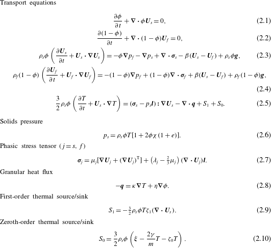
Transport equations and constitutive relations of the GTSH KT-TFM. The solution variables are the solids concentration,
 $\unicode[STIX]{x1D719}$
, the solids and fluid velocity vectors,
 $\boldsymbol{U}_{j}=(u_{j},v_{j},w_{j})^{\text{T}}$
with
 $j=s,f$
, the fluid pressure,
 $p_{f}$
, and the granular temperature,
 $T$
. Additionally,
 $\unicode[STIX]{x1D70C}_{j}$
is the phasic density,
 $\boldsymbol{g}$
is the gravity vector,
 $e$
is the restitution coefficient,
 $d_{p}$
is the particle diameter and
 $m$
is the particle mass.

This study utilizes a two-fluid model (TFM) to solve gas–solid flow in a state of fluidization or sedimentation in a fully periodic domain. The solids-phase transport coefficients and constitutive relations are closed with a KT approach. We use the KT-TFM of Garzó et al. (Reference Garzó, Tenneti, Subramaniam and Hrenya2012) (hereafter referred to as GTSH). Unlike previous KT models for particulate flows, the instantaneous gas–solid interaction force appearing in the starting Enskog equation is decomposed into three components: (i) a mean drag force (proportional to
 $\unicode[STIX]{x1D6FD}$
in table 1) that models the interfacial momentum transfer due to a difference in mean relative velocities, (ii) a thermal drag force (proportional to
 $\unicode[STIX]{x1D6FE}$
in table 4) that models the dissipation of granular temperature (a measure of the fluctuating kinetic energy of the solids phase) due to the fluid phase, and (iii) a neighbour effect (proportional to
 $\unicode[STIX]{x1D709}$
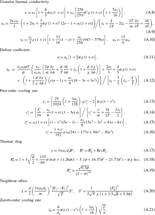
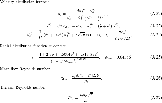
in table 5), which is a source of granular temperature due to the fluid and the presence of nearby particles, i.e. it is necessarily both a multiphase and multi-particle contribution. For the sake of brevity, only the governing and constitutive equations of the KT-TFM are given in table 1. The additional relations needed to fully specify the GTSH model are provided in tables 3–5 in appendix A along with a discussion of the slight differences between closures used here and those originally proposed by Garzó et al. (Reference Garzó, Tenneti, Subramaniam and Hrenya2012). In §§ 2.1.1, 2.1.2 and 2.1.3 we provide a review of the relevant assumptions and approximations that impact the limitations of the GTSH theory.
2.1.1 Particle and collision properties
It is assumed that particles are perfectly spherical and monodisperse. Normal dissipation resulting from particle–particle collisions is assumed to be characterized by a single, constant coefficient of restitution,
 $e$
. Furthermore, the collisions are assumed to be instantaneous and binary. The particle surface is assumed to be perfectly smooth, i.e. tangential dissipation due to particle–particle friction is zero. These idealized particle and collisional properties are shared by the DNS, thereby providing a straightforward (apples-to-apples) comparison between DNS and GTSH theory.
2.1.2 Fluid properties
The fluid phase is assumed to be incompressible,
 $\unicode[STIX]{x2202}\unicode[STIX]{x1D70C}_{f}/\unicode[STIX]{x2202}t+\boldsymbol{U}_{f}\boldsymbol{\cdot }\unicode[STIX]{x1D735}\unicode[STIX]{x1D70C}_{f}=0$
, which is the reason that (2.1) and (2.2) are independent of density. In this work, the fluid properties,
 $\unicode[STIX]{x1D70C}_{f}$
,
 $\unicode[STIX]{x1D707}_{f}$
and
 $\unicode[STIX]{x1D706}_{f}$
are further assumed to be constants in a given simulation. In typical fashion, bulk compressibility is neglected by assuming
 $\unicode[STIX]{x1D706}_{f}=2\unicode[STIX]{x1D707}_{f}/3$
. Both fluid-phase assumptions are also matched in the DNS. It should also be mentioned that in the KT-TFM ‘subgrid’ contributions to the fluid-phase stress tensor, such as those resulting from ‘microscopic’ particle-induced turbulence, are not considered here. However, small-scale fluctuations in the fluid velocity cause by individual particles are inherently captured by the DNS approach and, hence, do not require modelling. Note that ‘mesoscopic’ or ‘macroscopic’ fluctuations resulting from variations in mean flow, or clustering-induced turbulence (Capecelatro et al.
Reference Capecelatro, Desjardins and Fox2015), are actively resolved by solving the full transient, three-dimensional (3-D) KT-TFM equations in the simulations.
2.1.3 Kinetic equation and its solution
Although several options exist for obtaining the necessary constitutive relations and transport coefficients from a kinetic equation, the Chapman–Enskog expansion has been the most prevalent systematic method to date (Goldhirsch Reference Goldhirsch2003). The Chapman–Enskog method assumes that the kinetic equation has a normal solution, e.g. that the velocity distribution function depends on space and time only through a dependence on
 $\unicode[STIX]{x1D719}$
,
 $\boldsymbol{U}_{s}$
, and
 $T$
(Chapman & Cowling Reference Chapman and Cowling1970), which is constructed using a perturbation expansion about a uniformity (small) parameter. The uniformity parameter used in the Chapman–Enskog method is the Knudsen number,
 $Kn$
, which is a measure of the mean free path of the particles relative to the strength (inverse length scale) of spatial gradients of the hydrodynamic variables. The GTSH model is expanded to first order in
 $Kn$
, i.e. Navier–Stokes order. Additionally, the scaled distribution function is approximated by expanding about the Maxwellian distribution with Sonine polynomials (van Noije & Ernst Reference van Noije and Ernst1998). The GTSH theory considers a first-order Sonine approximation measuring the Maxwellian deviation through the kurtosis (A 22). Although never explicitly stated, an over-arching assumption of this approach is that the distribution function should be predominantly determined by particle collisions (i.e. high thermal Stokes number). It is worth mentioning that DNS does not rely on any of the assumptions related to the kinetic equation or its solution since all particle dynamics, including collisions, are directly resolved.
2.2 Numerical solution of the KT-TFM
The GTSH KT-TFM is solved numerically using the open-source MFiX CFD code developed at the National Energy Technology Laboratory (https://mfix.netl.doe.gov/). MFiX solves the discretized transport equations with the finite volume method. The spatial discretization employs a staggered grid and an upwinded variable extrapolation scheme with a flux limiter. All simulations in this work were performed with the MUSCL flux limiter (van Leer Reference van Leer1979; Waterson & Deconinck Reference Waterson and Deconinck2007) on a uniform grid of
 $N_{x}=N_{z}=12$
and
 $N_{y}=50$
. Although the grid is uniform, it is not exactly cubic and the exact grid spacing
 $\unicode[STIX]{x1D6E5}_{i}=L_{i}/N_{i}$
for
 $i=x,y,z$
, changes slightly depending on the Archimedes number, see § 2.4 below. For both Archimedes numbers, the non-dimensionalized grid size,
 $\unicode[STIX]{x1D6E5}^{\ast }=(\unicode[STIX]{x1D6E5}_{x}\times \unicode[STIX]{x1D6E5}_{y}\times \unicode[STIX]{x1D6E5}_{z})^{1/3}/d_{p}$
, is approximately 0.7 which was determined to be necessary after carrying out a systematic grid dependence study of a test case. Such a fine grid is approximately an order of magnitude smaller than previously found to be necessary for grid-insensitive solutions (Agrawal et al.
Reference Agrawal, Loezos, Syamlal and Sundaresan2001; Wang et al.
Reference Wang, van der Hoef and Kuipers2009; Fullmer & Hrenya Reference Fullmer and Hrenya2016). It is believed that such a high level of numerical resolution is needed here due to the small system size; specifically, large spatial gradients at cluster interfaces account for a larger portion of the total domain in this study (Li et al.
Reference Li, Wang, Rogers, Zhou and Ge2017). Time advancement is semi-implicit with a SIMPLE-type algorithm (Patankar Reference Patankar1980) for pressure–velocity coupling. The temporal discretization is first-order Euler with adaptive time stepping. A maximum time step of is specified, however in order to meet the tolerance limits, the code-limited time step is typically one to two orders of magnitude smaller than the maximum time step.
2.3 DNS method
The SUSP3D code developed by Ladd and co-workers (Ladd & Verberg Reference Ladd and Verberg2001; Nguyen & Ladd Reference Nguyen and Ladd2002) is used in this study to simulate the dynamics of fully periodic sedimentation/fluidization. This code uses a D3Q19 lattice Boltzmann velocity model and a two-relaxation-time collision operator to solve fluid flow on a uniform, space filling, cubic lattice. Incompressible flow is recovered with second-order accuracy with respect to the lattice Mach number,
 $Ma=u/c_{s}$
, where
 $u$
is the fluid velocity and
 $c_{s}=1/\sqrt{3}$
is the lattice speed of sound. When a fluid population crosses a fluid–solid interface, the linked-bounce-back rule is applied to return the fluid population back to the fluid domain, recovering the no-slip boundary condition. The momentum exchanged between the fluid and a particle through bounce-back is accumulated over the surface of the particle to give the fluid–particle force. This force is then used to update the particles velocity according to Newton’s law of motion.
For close pairs of particles, analytical expressions of lubrication interactions are imposed onto lattice Boltzmann solutions to ensure that lubrication interactions between particles are correctly captured (Nguyen & Ladd Reference Nguyen and Ladd2002). As analytical expressions contain singularities when the gap between particles approaches zero, a lubrication cutoff,
 $\unicode[STIX]{x1D716}$
is specified. This cutoff sets maximum values on the lubrication force and torque, and reduces the stiffness of the velocity update. As in the assumptions used to derive the GTSH KT-TFM, collisions between particles are treated as hard sphere collisions with a normal restitution coefficient. Tangential restitution due to friction was not considered in the simulations.
Parameters used in the DNS.
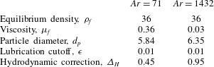
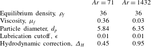
Table 2 lists the properties of the lattice fluid, diameters of particles and lubrication cutoffs that were employed in the simulations. Note that the diameter
 $d_{p}$
is the effective hydrodynamic diameter, which is different from the geometric diameter,
 $d_{p}^{0}$
, used to distinguish fluid and solid nodes on the computational lattice. Generally
 $d_{p}>d_{p}^{0}$
, because the collection of solid nodes mapped by
 $d_{p}^{0}$
has a rough interface that comes from the staircase representation of a sphere. The difference between
 $d_{p}$
and
 $d_{p}^{0}$
, the hydrodynamic correction
 $\unicode[STIX]{x1D6E5}_{H}$
, is typically established through drag calibration (Ladd & Verberg Reference Ladd and Verberg2001), and is always less than one lattice spacing. As one increases
 $d_{p}$
and
 $d_{p}^{0}$
, the need for a hydrodynamic correction decreases, as the sphere is now represented by more lattice units (i.e. higher resolution). The choice of
 $d_{p}$
is generally based on the balance between computational cost and accuracy. In this study, we tested a higher resolution
 $d_{p}=10$
for selected cases, and the results were identical to those obtained using the lower
 $d_{p}$
listed in table 2. It was also tested and confirmed that the DNS results are essentially not affected by the selection of
 $\unicode[STIX]{x1D716}$
.
2.4 System description
The system considered is a uniform suspension in a fully periodic domain undergoing infinite sedimentation or fluidization. A constant body force, i.e. gravity, acts only in the negative vertical
 $y$
-direction. In the KT-TFM simulations, the fluid pressure is assumed to be decomposed into a fluctuating (local) component superimposed on a mean linear gradient. The mean fluid pressure gradient opposes the body force and supports the weight of the suspension,
 $$\begin{eqnarray}-\!\frac{\unicode[STIX]{x2202}P_{f}}{\unicode[STIX]{x2202}y}=(\langle \unicode[STIX]{x1D719}\rangle \unicode[STIX]{x1D70C}_{s}+(1-\langle \unicode[STIX]{x1D719}\rangle )\unicode[STIX]{x1D70C}_{f})|\boldsymbol{g}|\end{eqnarray}$$
so that no net force acts on the mixture in the
 $y$
-direction. The angle brackets in (2.11) indicate an averaging over the entire domain. The pressure gradient is imposed on the system numerically by specifying a pressure-drop boundary condition in the
 $y$
-direction. In DNS, a body force equivalent to that specified by (2.11) is applied to the fluid to ensure that the net force on the mixture in the
 $y$
-direction is zero. No forces are applied in the transverse
 $x$
- and
 $z$
-directions and standard periodic boundary conditions are used. Since the system is fully periodic, the global (system) concentration,
 $\langle \unicode[STIX]{x1D719}\rangle$
, does not change in time.
With the specification of (2.11) one can calculate the base state, i.e. the homogeneous (stable) steady state, which will be an important metric for comparison with the numerical solutions of the complete (transient and three-dimensional) GTSH KT-TFM. The mixture momentum equation, (2.3)
 $+$
(2.4), reduces to (2.11). The difference momentum equation, (2.3)–(2.4), can be rearranged to give the mean velocity difference in the vertical direction:
 $$\begin{eqnarray}|v_{s}^{({\mathcal{H}})}-v_{f}^{({\mathcal{H}})}|=\frac{\unicode[STIX]{x0394}\unicode[STIX]{x1D70C}|\boldsymbol{g}|d_{p}^{2}}{18\unicode[STIX]{x1D707}_{f}F^{\ast }}=\frac{u_{\infty }}{F^{\ast }},\end{eqnarray}$$
where
 $u_{\infty }$
is the terminal Stokes velocity of a single particle in an infinite medium and
 $F^{\ast }$
is the mean drag law (A 1) and the
 $({\mathcal{H}})$
superscript denotes the homogeneous state. In §§ 3 and 4, it will be important to distinguish between values calculated analytically from the KT-TFM assuming homogeneity and those calculated from the results of CFD simulations of the KT-TFM which may be far from homogeneous. The transverse velocities in the homogeneous state are all zero:
 $u_{s}^{({\mathcal{H}})}=u_{f}^{({\mathcal{H}})}=w_{s}^{({\mathcal{H}})}=w_{f}^{({\mathcal{H}})}=0$
. Note that (2.12) only prescribes the magnitude of the velocity difference, not the phasic velocity values. The mixture continuity equation, (2.1)
 $+$
(2.2), states only that the total volumetric flux should be a constant,
 $$\begin{eqnarray}j_{y}^{({\mathcal{H}})}=[\unicode[STIX]{x1D719}v_{s}+(1-\unicode[STIX]{x1D719})v_{f}]^{({\mathcal{H}})}=\text{const.}\end{eqnarray}$$
In theory, the absolute values of the phasic velocities are arbitrary: hence the lack of distinction between sedimentation or fluidization in a fully periodic domain. However, to satisfy the
 $Ma$
criterion in the DNS, the velocities should be minimized and thus the choice
 $j_{y}^{({\mathcal{H}})}=0$
was selected and also used in the KT-TFM simulations for consistency. With
 $j_{y}^{({\mathcal{H}})}=0$
, equation (2.12) yields
 $v_{s}^{({\mathcal{H}})}=-(1-\langle \unicode[STIX]{x1D719}\rangle )u_{\infty }/F^{\ast }$
and
 $v_{f}^{({\mathcal{H}})}=\langle \unicode[STIX]{x1D719}\rangle u_{\infty }/F^{\ast }$
(note that
 $\unicode[STIX]{x1D719}^{({\mathcal{H}})}=\langle \unicode[STIX]{x1D719}\rangle$
). In the homogeneous state, the granular temperature equation (2.5) reduces to the algebraic relation
 $S_{0}=0$
or,
 $$\begin{eqnarray}\left[\unicode[STIX]{x1D709}=\frac{2\unicode[STIX]{x1D6FE}}{m}T+\unicode[STIX]{x1D701}_{0}T\right]^{({\mathcal{H}})},\end{eqnarray}$$
which describes how granular temperature generated by the neighbour effect is balanced the by the dissipation due to thermal drag and inelasticity (if
 $e<1$
).
For both numerical methods, the fluid and particles are initially at rest and accelerated by body forces to achieve the quasi-steady state of sedimentation. Though by different means, both methods enforce
 $\langle j_{y}\rangle =0$
dynamically throughout calculations to avoid drift caused by round-off error. To provide an initial perturbation in the KT-TFM simulations consistent with DNS randomly distributed particles are generated at initialization and filtered into solids concentration on the CFD grid with a simple Gaussian filter. Furthermore, in the KT-TFM simulations a negligibly small initial granular temperature is prescribed to avoid singularities in the constitutive equations. In this manner, the KT-TFM and DNS methods were initialized as similarly as possible.
Seven non-dimensional parameters characterize the system: the Archimedes number,
 $Ar=\unicode[STIX]{x1D70C}_{f}\unicode[STIX]{x0394}\unicode[STIX]{x1D70C}|\boldsymbol{g}|d_{p}^{3}/\unicode[STIX]{x1D707}_{f}^{2}$
, characterizing the ratio of gravity-to-viscous forces, the density ratio,
 $\unicode[STIX]{x1D70C}^{\ast }=\unicode[STIX]{x1D70C}_{s}/\unicode[STIX]{x1D70C}_{f}$
, the mean concentration,
 $\langle \unicode[STIX]{x1D719}\rangle$
, the coefficient of restitution,
 $e$
, and the system size in each direction,
 $L_{i}^{\ast }=L_{i}/d_{p}$
where
 $i=x,y,z$
. Two Archimedes numbers considered in this study,
 $Ar=71$
and 1432, lead to approximately one order of magnitude of variation in mean-flow Reynolds numbers, equation (A 26). (Note that (2.12) can be easily non-dimensionalized into the form
 $Re_{m}^{({\mathcal{H}})}=(1-\langle \unicode[STIX]{x1D719}\rangle )Ar/18F^{\ast }$
). The density ratio serves as the control parameter and was varied from 10 to 1000. Four mean concentrations are studied,
 $\langle \unicode[STIX]{x1D719}\rangle =0.10$
, 0.15, 0.25 and 0.40 and two values of the restitution coefficient are used,
 $e=0.9$
and 1.0. Here, we primarily focus on the results obtained in the elastic case (
 $e=1.0$
) as inelasticity does not significantly affect the results as discussed in § 4.6. The system size varies slightly between the two Archimedes number cases. For the case
 $Ar=71$
:
 $L_{x}^{\ast }=L_{z}^{\ast }=8.56$
and
 $L_{y}^{\ast }=34.2$
. For the
 $Ar=1432$
case:
 $L_{x}^{\ast }=L_{z}^{\ast }=8.656$
and
 $L_{y}^{\ast }=34.624$
. In both instances, the domain size is very small – a consequence of the large computational cost associated with DNS. Capecelatro et al. (Reference Capecelatro, Desjardins and Fox2015) recommend that the domain size in the flow direction be at least
 $L_{y}^{\ast }\approx 0.2\unicode[STIX]{x1D70C}^{\ast }Ar$
(assuming
 $\unicode[STIX]{x1D70C}^{\ast }\gg 1$
). In this work,
 $0.2\unicode[STIX]{x1D70C}^{\ast }Ar$
ranges from 142 to 286 400 – orders of magnitude larger than
 $L_{y}^{\ast }$
considered here – so that the periodic boundaries influence the development of the instabilities. Therefore, when clustering occurs it forms a significantly different structure than observed in larger, truly unbounded domains, e.g. Capecelatro et al. (Reference Capecelatro, Desjardins and Fox2015), Capecelatro, Desjardins & Fox (Reference Capecelatro, Desjardins and Fox2016). However, the variety of structures observed as a result of the small system provide an equally, if not more, stringent test of the KT-TFM than traditional clustering alone, as shown in § 3.
2.5 Averaging operations
A few averaging operations that will be used in the following sections are formally defined here. Consider a general, arbitrary variable
 $f_{j}$
associated with phase-
 $j$
which is a function of space and time. The volume average,
 $$\begin{eqnarray}\langle f_{j}\rangle (t^{\ast })=\frac{1}{L_{x}^{\ast }L_{y}^{\ast }L_{z}^{\ast }}\int _{0}^{L_{z}^{\ast }}\int _{0}^{L_{y}^{\ast }}\int _{0}^{L_{x}^{\ast }}f_{j}(\boldsymbol{x}^{\ast },t^{\ast })\,\text{d}x^{\ast }\,\text{d}y^{\ast }\,\text{d}z^{\ast },\end{eqnarray}$$
defines the global or system-averaged quantity. When comparing with the results of DNS, continuum flow variables, e.g. solids velocity, must be Favre or concentration weighted,
 $$\begin{eqnarray}\langle \langle f_{s}\rangle \rangle (t^{\ast })=\frac{\langle \unicode[STIX]{x1D719}f_{s}\rangle (t^{\ast })}{\langle \unicode[STIX]{x1D719}\rangle (t^{\ast })}\quad \text{and}\quad \langle \langle f_{f}\rangle \rangle (t^{\ast })=\frac{\langle (1-\unicode[STIX]{x1D719})f_{f}\rangle (t^{\ast })}{1-\langle \unicode[STIX]{x1D719}\rangle (t^{\ast })},\end{eqnarray}$$
denoted here by double brackets. Finally, the system is simulated in a statistical steady state and it is frequently desired to report time-averaged values,
 $$\begin{eqnarray}\overline{f_{j}}(\boldsymbol{x}^{\ast })=\frac{1}{t_{2}^{\ast }-t_{1}^{\ast }}\int _{t_{1}^{\ast }}^{t_{2}^{\ast }}f_{j}(\boldsymbol{x}^{\ast },t^{\ast })\,\text{d}t^{\ast }\end{eqnarray}$$
denoted with an overbar. The non-dimensional time is defined here as
 $t^{\ast }=t\unicode[STIX]{x1D708}_{f}/d_{p}^{2}$
. Since DNS is extremely computationally expensive, the time averaging windows are minimized by beginning time averaging as soon as the quasi-steady state is reached and terminating each simulation when a sufficient amount of statistics have been collected, typically controlled by the higher-order statistics. Five replicates (otherwise identical simulations with a different randomization of initial particle distribution) were run for each condition. The DNS results provided in § 4 represent the average of the five replicates with error bars signifying the standard deviation between the replicates. The KT-TFM simulations are carried out to
 $t^{\ast }=2000$
for
 $Ar=71$
and to
 $t^{\ast }=500$
for
 $Ar=1432$
. In both cases, the data are split into ten equal length segments. The first segment is neglected to avoid any transient data associated with the transition from the initially static but perturbed state to the statistically steady state. The remaining nine segments are time averaged and used to calculate the mean and standard deviation, the latter of which is represented by error bars throughout this work except in figure 11 where specifically noted otherwise.
3 Results: flow structure
In this section, we present a qualitative comparison on the degree of inhomogeneity between KT-TFM and DNS. In a previous work on the HCS (Mitrano et al.
Reference Mitrano, Zenk, Benyahia, Galvin, Dahl and Hrenya2014), an L
 $_{\infty }$
-norm, termed
 $\unicode[STIX]{x0394}\unicode[STIX]{x1D719}_{max}$
, was used to differentiate the inhomogeneous (clustered) state from the homogeneous state. The HCS is in a state of constant decay and the
 $\unicode[STIX]{x0394}\unicode[STIX]{x1D719}_{max}$
was studied as a function of time. For the statistically steady sedimenting system studied here, a single metric indicating the degree of inhomogeneity at the steady state is more appropriate. Therefore, the inhomogeneity metric
 $\unicode[STIX]{x0394}\unicode[STIX]{x1D719}_{max}$
is taken here as
 $$\begin{eqnarray}\unicode[STIX]{x0394}\unicode[STIX]{x1D719}_{max}=\overline{\left(\frac{\max \unicode[STIX]{x1D719}-\min \unicode[STIX]{x1D719}}{\langle \unicode[STIX]{x1D719}\rangle }\right)}.\end{eqnarray}$$
 $\unicode[STIX]{x0394}\unicode[STIX]{x1D719}_{max}$
expresses the average maximum spread of the concentration field normalized by the mean concentration and takes a range of values from zero (perfectly homogeneous) to
 $\unicode[STIX]{x1D719}_{max}/\langle \unicode[STIX]{x1D719}\rangle$
, where
 $\unicode[STIX]{x1D719}_{max}$
is the random close-packed concentration limit in the radial distribution function (A 25).
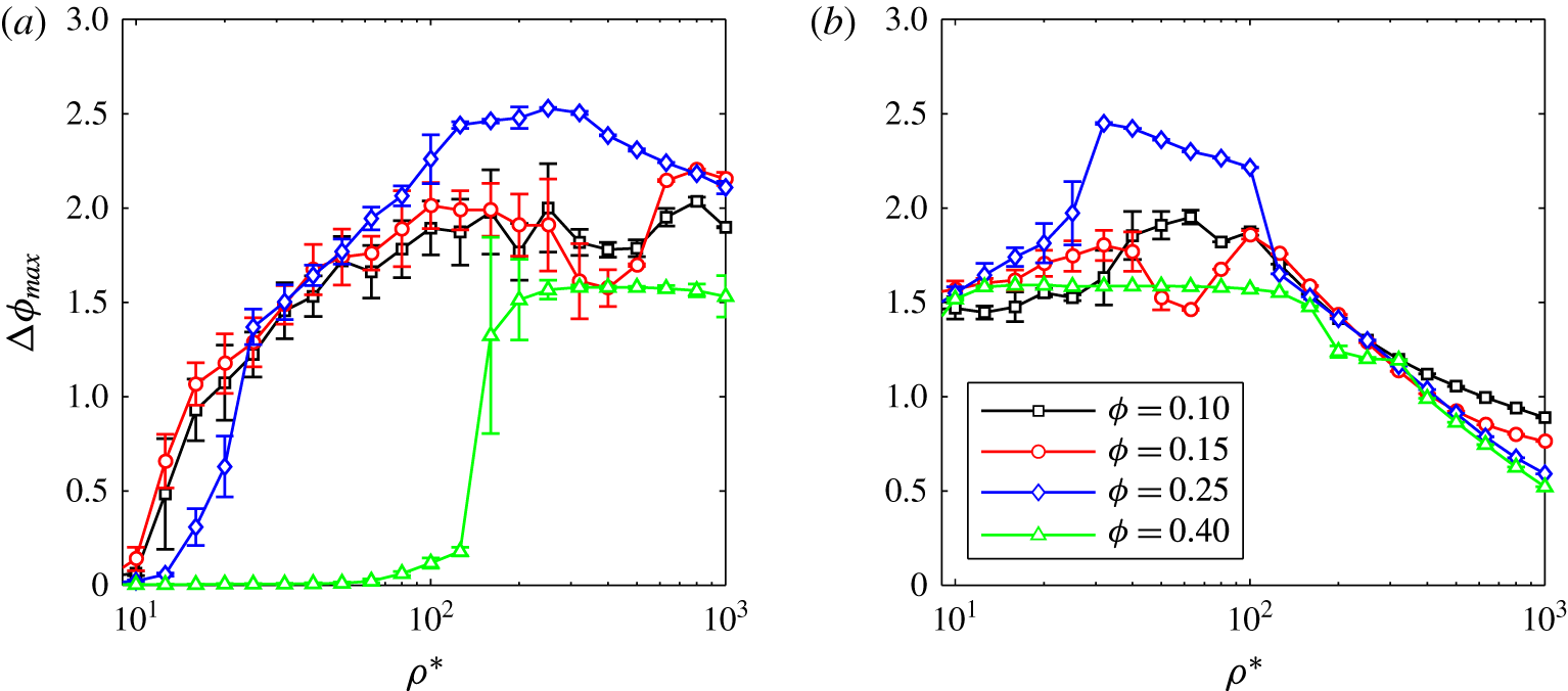
Maximum normalized concentration difference in the KT-TFM simulations as a function of density ratio for
 $e=1$
and (a)
 $Ar=71$
and (b)
 $Ar=1432$
at mean concentrations of
 $\langle \unicode[STIX]{x1D719}\rangle =0.1$
(black), 0.15 (red), 0.25 (blue) and 0.40 (green).

Figure 1 presents
 $\unicode[STIX]{x0394}\unicode[STIX]{x1D719}_{max}$
for all inelastic KT-TFM simulations at (a)
 $Ar=71$
and (b)
 $Ar=1432$
, respectively. In general, the main trends of the two
 $Ar$
cases are opposite. At low
 $Ar$
and the three lowest concentrations,
 $\langle \unicode[STIX]{x1D719}\rangle =0.10$
, 0.15 and 0.25,
 $\unicode[STIX]{x0394}\unicode[STIX]{x1D719}_{max}$
is near zero (indicating a homogeneous state) at the lowest density ratios and increases to a clustered state with increasing density ratio. For
 $\langle \unicode[STIX]{x1D719}\rangle =0.40$
, this system remains essentially homogenous to a density ratio of approximately 100, at which point the system abruptly transitions to an inhomogeneous state. At high
 $Ar$
, the systems begin (i.e. at lower density ratio) in an inhomogeneous state and
 $\unicode[STIX]{x0394}\unicode[STIX]{x1D719}_{max}$
begins to decay at a density ratio of approximately 100. It should be pointed out that this re-homogenization at
 $Ar=1432$
is considerably smoother than the onset of clustering at
 $Ar=71$
. Although
 $\unicode[STIX]{x0394}\unicode[STIX]{x1D719}_{max}$
can be used as a quick gauge of whether or not a system is inhomogeneous, it cannot provide information on how a system is inhomogeneous. Different types of clustered states are illustrated via instantaneous snapshots of the concentration fields for representative cases in the remainder of this section. Animations of each system also reveal that the observed behaviour was significantly more complex than simply homogeneous/inhomogeneous (stable/clustered), see supplementary movies for example animations available at https://doi.org/10.1017/jfm.2017.295.
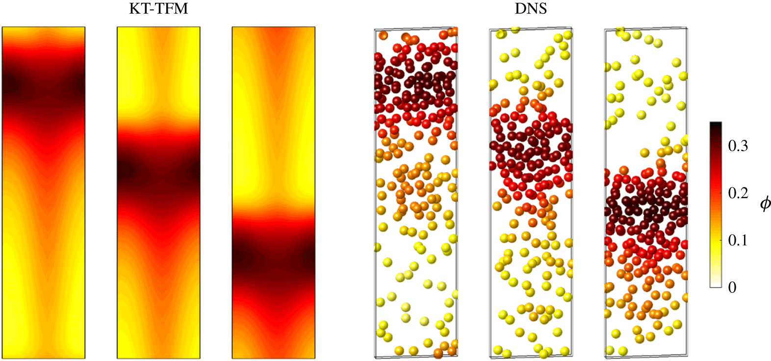
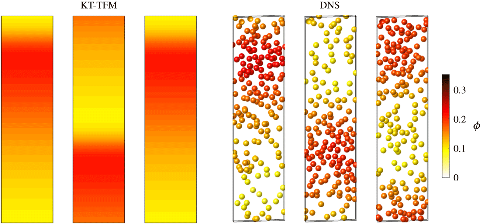
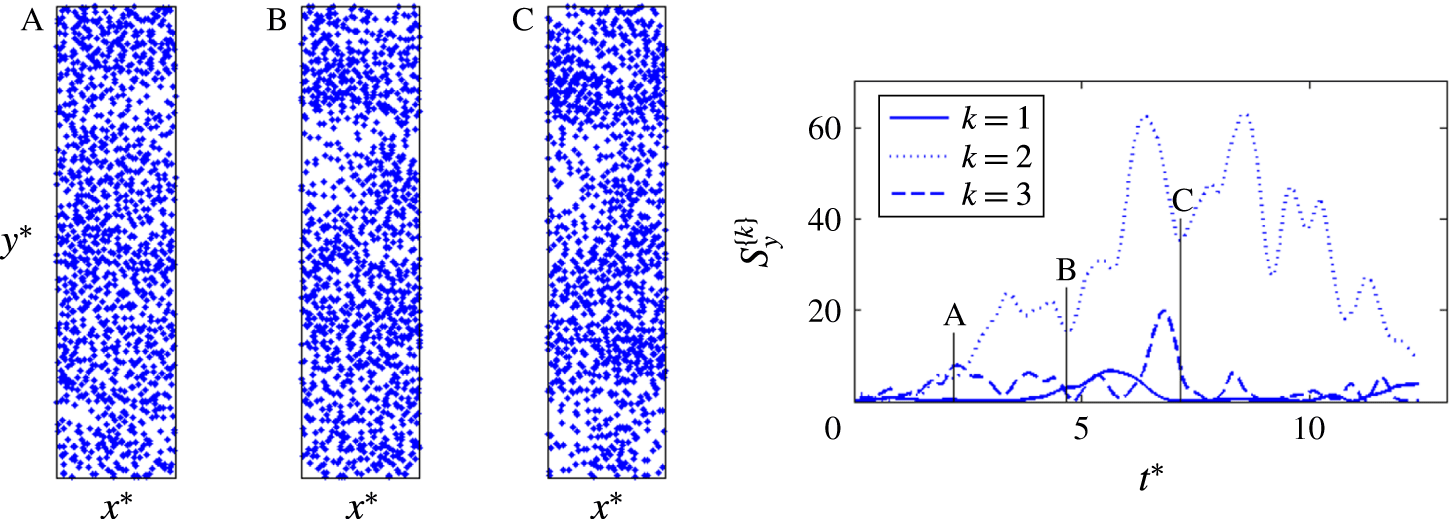
Further insight into the types of structures present in these small-scale sedimenting systems is provided by instantaneous snapshots of the distributions of concentration (for KT-TFM) and particles (for DNS) for representative cases. For each set of images in figures 2–4 a corresponding animation is provided in supplementary movies 1–6. Broadly speaking, approximately four different regimes have been observed in the KT-TFM: (i) steady and nearly homogeneous, (ii) unsteady and chaotic, (iii) steady 2-D plug and (iv) steady 1-D plug. Because the transitions from one regime to another are always gradual, it is not easy to quantitatively demarcate the transitions. Here we present the typical structures of each regime, except that of the first regime due to its trivial nature. Analysis of the transition to the plug flow is considered in § 4.4. It should be noted that on the DNS side, as particle locations and flow fields are always fluctuating, there is no stable, steady regime (i) as in the KT-TFM simulations.
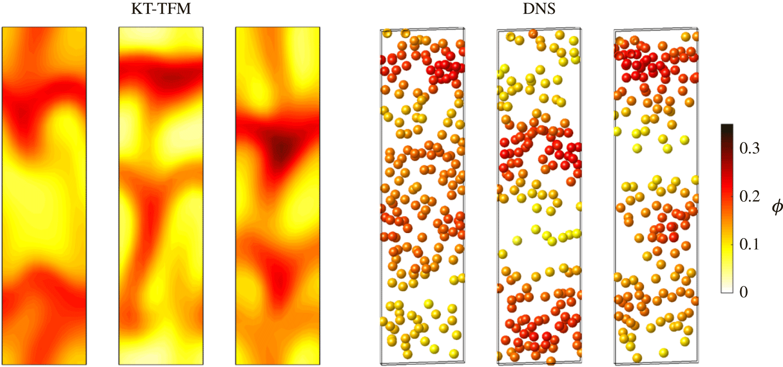
Chaotic regime: instantaneous distribution of KT-TFM solids concentration and DNS particle locations. Concentration field shown in
 $xy$
-plane at the
 $z$
-centreline. Particles shown in
 $d_{p}$
-thick slice about the
 $z$
-centreline and are coloured by filtered volume fraction. Both contours and particles indicate a concentration range from 0 to 0.35 by light yellow to dark red colours. Consecutive panels are separated by
 $\unicode[STIX]{x1D6FF}t^{\ast }=1.5$
. Conditions are:
 $Ar=1432$
,
 $\langle \unicode[STIX]{x1D719}\rangle =0.15$
,
 $e=1.0$
, and
 $\unicode[STIX]{x1D70C}^{\ast }=32$
(KT-TFM), 30 (DNS).

The unsteady and ‘chaotic’ regime, as illustrated in figure 2, occurs at intermediate density ratios after the near-homogeneous regime in the lower
 $Ar=71$
case and at the lowest density ratios studied in the higher
 $Ar=1432$
case. In the KT-TFM simulations, the departure from near-homogeneous to observable flow structures coincides with the abrupt increase in
 $\unicode[STIX]{x0394}\unicode[STIX]{x1D719}_{max}$
in figure 1 for
 $Ar=71$
. The regime is characterized by a highly dynamic state in which identifiable structures change shape rapidly and frequently coalesce with other structures or vanish. Quotations are used around chaotic because we have not attempted to quantify or otherwise verify a chaotic state and simply mean that the flow appears to have many of the hallmarks often associated with chaos. We note however that a recent study of clustering in a larger sedimenting system predicted with the GTSH KT-TFM was shown to possess a positive Lyapunov exponent (Fullmer & Hrenya Reference Fullmer and Hrenya2017a
). The highest frequencies of the dynamics occur at the lower density ratio side of each chaotic regime, although before the onset of homogeneity. With increasing density ratio the horizontal structures become more pronounced which can be clearly identified in figure 2. Both KT-TFM and DNS images show two horizontal, plug-like structures in the domain. Although there are frequently two identifiable plugs, one is typically ‘stronger’ (denser) while other is in a regenerative state. At the first instance shown (left most panel), the plug near the top of the domain is the dominant plug. As the simulations continue, the plugs fall through the domain and are broken by the fluid causing the particles to spill out and decreasing the strength. By the third panel, the originally stronger plug has become the weaker one (panels left to right are separated by
 $\unicode[STIX]{x1D6FF}t^{\ast }=1.5$
for both KT-TFM and DNS). Conversely, the lower plugs have passed through the bottom of the domain (and re-emerged at the top due to the periodic boundary condition) and have become the dominant plug in the third panel. The cycle of destruction and rebirth of the horizontal structures continually repeats itself. It should be noted that while a repetitive pattern is distinguishable through visible inspection, the spatial configuration is by no mean regular, i.e. the plugs are similar but not identical in shape, indicating that the system is still in a chaotic state.
Two-dimensional plug regime: same as figure 2 except at
 $\unicode[STIX]{x1D70C}^{\ast }=100$
(both KT-TFM and DNS).

One-dimensional plug regime: same as figure 2 except at
 $\unicode[STIX]{x1D70C}^{\ast }=1000$
(both KT-TFM and DNS).

As the density ratio continues to increase, the fluid phase no longer has enough inertia to break up plug structures and at some point in
 $\unicode[STIX]{x1D70C}^{\ast }$
the transverse plug structures begin to persist throughout simulations. At this point, only a single plug is present at a given time (regime (iii)). The persistent plug structure is displayed in figure 3 for
 $\unicode[STIX]{x1D70C}^{\ast }=100$
(and the same remaining conditions as in figure 2). It can be seen that the maximum and minimum concentrations in the domain are approximately the same in figures 2 and 3 and, hence, the magnitudes or even trends of
 $\unicode[STIX]{x0394}\unicode[STIX]{x1D719}_{max}$
in figure 1 do not change appreciably from the chaotic to plug regimes. Since the plug spans the domain in the lateral direction, the fluid must flow though the dense region, which will have an impact on the global mean-flow properties. Clustering is typically associated with ‘flow bypass’, which will not occur when the fluid flow is forced to penetrate plugs spanning the entire width. Originally discussed by Li & Kwauk (Reference Li and Kwauk2001), flow bypass is the preferential flow of the fluid phase around dense clusters which tends reduce the overall drag. For the conditions presented in figure 3, the plugs are quite stable in a nonlinear sense (if the system were linearly stable, it would decay to the homogeneous state) and the repeated passing of the plug appears to be a travelling wave limit cycle. The plug in the KT-TFM simulations of figure 3 shows a clearly identifiable funnel structure emanating from the bottom and wrapping around the domain to join the top. A similar pattern often appears in the DNS, although it is more difficult to identify in the instantaneous snapshots than the videos as it is more irregular in the DNS than in the KT-TFM. Very close to the transition from the chaotic region, i.e. at
 $\unicode[STIX]{x1D70C}^{\ast }$
when the plugs are just strong enough to resist being fragmented by the fluid, the KT-TFM simulations also predict that the funnel ‘wiggles’ or oscillates in the transverse dimensions. Owing to this multi-dimensional nature of the plugs, this regime is identified as ‘2-D’ plugs. Although the qualitative similarities between the KT-TFM and DNS results are very good, some minor quantitative differences can be observed in figure 3. For example, comparing the location of the centre of plugs in the three panels indicates an over-prediction of the speed of the plug by KT-TFM.
The multi-dimensional structure of the plug decays as the density ratio is further increased. At a given point in
 $\unicode[STIX]{x1D70C}^{\ast }$
, the 2-D shape of the plug is lost entirely and a 1-D travelling wave limit cycle appears; see figure 4. A 1-D wave was originally predicted by Anderson & Jackson (Reference Anderson and Jackson1968) to be the most unstable perturbation to a uniform suspension. As the density ratio continues to increase, the plug grows in thickness and decreases in amplitude (i.e. maximum concentration of plug). Both features can be observed in figure 4 for
 $\unicode[STIX]{x1D70C}^{\ast }=1000$
(and the same remaining conditions as in figures 2 and 3). The decreasing amplitude of the plug directly coincides with the decay of
 $\unicode[STIX]{x0394}\unicode[STIX]{x1D719}_{max}$
seen previously in figure 1 for
 $Ar=1432$
at high density ratios. Some exploratory studies on a coarser grid indicate that this decay continues asymptotically, slowly approaching a perfectly homogeneous state as the density ratio approaches infinity. As in figure 3, the speed of the plug in figure 4 is slightly over-predicted by KT-TFM which shows the plug has wrapped around within the window
 $\unicode[STIX]{x1D6FF}t^{\ast }=3$
, while the DNS plug has not quite completely returned to its original position. Nevertheless, the qualitative agreement between the two is again outstanding as the main features, e.g. loss of 2-D structure, decrease in (concentration) amplitude, increase in thickness and increase in speed compared to figure 3, are all captured by the KT-TFM theory. In § 4.4 the regime transition predicted by KT-TFM is quantified and compared to the DNS results.
The three non-trivial regimes shown in figures 2–4 are all taken from the higher
 $Ar$
simulations. It should be noted that the trivial (homogeneous) case was not observed for
 $Ar=1432$
and the 1-D plug regime was not observed for
 $Ar=71$
. However, exploratory simulations on a coarser grid indicate that the 1-D regime is also observed for
 $Ar=71$
at a density ratio larger then considered in this study (in some instances, just slightly larger). Therefore, it is believed that the same instability patterns and transitions occur at both values – and likely a wide range – of
 $Ar$
offset in density ratio, although such a phase-space-spanning study has not been performed.
It has been shown in this section that the KT-TFM is able to capture the unstable regimes observed in the DNS of fully periodic sedimentation. Due to the small size of the computational domain considered, several distinct structures were identified: chaotic, width-spanning 2-D plugs and width-spanning 1-D plugs. While only qualitative in nature, the level of agreement seen here is remarkable – the quasi-steady states simulated here are considerably more complex than the previous near-linear clustering/not-clustering states studied in the HCS (Mitrano et al. Reference Mitrano, Zenk, Benyahia, Galvin, Dahl and Hrenya2014). In the following section § 4, we probe deeper by making direct quantitative comparisons between KT-TFM and DNS results of mean-flow quantities, fluctuating quantities and regime transition.
4 Results: time-averaged flow properties
4.1 Analysis of the Stokes number and the limit of GTSH theory
In the following §§ 4.2–4.4, the KT-TFM and DNS results are directly compared quantitatively for two Archimedes numbers, several mean concentrations and a wide range of solid-to-fluid density ratios. In general, the best agreement is observed at the highest density ratios and a critical analysis of the assumptions overviewed in §§ 2.1.1–2.1.3 was carried out to determine why some regions of the phase space show better comparisons than others. A key benefit of comparing to ideal DNS numerical data is that the particle-phase properties and most of the fluid-phase properties are identical between KT-TFM and DNS. Moreover, complex physics commonly encountered in experiments (e.g. cohesion, humidity, etc.) are entirely neglected in both KT-TFM and the validation DNS data, providing as much of an ideal comparison as possible. The only physical condition that differs between KT-TFM and DNS is related to particle-induced turbulence; the fine grid used in the KT-TFM simulations actively capture cluster-induced turbulence, but small-scale fluctuations generated by the flow around individual particles are not specifically modelled. The impact of this discrepancy is gauged with Sato’s simple mixing length model for particle-induced turbulence,
 $\unicode[STIX]{x1D708}_{PIT}=C_{PIT}\unicode[STIX]{x1D719}d_{p}|\unicode[STIX]{x0394}U|$
, (Sato, Sadatomi & Sekoguchi Reference Sato, Sadatomi and Sekoguchi1981). Using the suggested value of
 $C_{PIT}=0.6$
, an empirical fitting coefficient originally developed for bubbly flows, and the homogeneous (stable) solution (2.12), the ratio
 $\unicode[STIX]{x1D708}_{PIT}/\unicode[STIX]{x1D708}_{f}$
ranges from 0.09 to 0.11 for
 $Ar=71$
and from 1.24 to 1.85 for
 $Ar=1432$
. Therefore, assumptions in the KT derivation, § 2.1.3, are the chief suspects for observed discrepancies. We focus here on the assumed particle distribution function (high thermal Stokes number assumption) and reserve a discussion of the small Knudsen number assumption for § 4.5.
As discussed in § 2.1.3, the GTSH theory allows for a non-Maxwellian velocity distribution function,
 $f$
. However, since
 $f$
is expressed as an expansion of Sonine polynomials (to first order),
 $f$
is expected to be near Maxwellian, its deviation from which is measured via (A 22) and relaxed predominantly by particle–particle collisions. In the context of a fluid–particle suspension, this assumption amounts to a requirement that the particle–particle (collisional) time scale should be much shorter than the fluid–particle (viscous relaxation) time scale (Koch Reference Koch1990) – i.e. a high thermal Stokes number (as defined below). We take the mean collision time to be the ratio of the mean free path due to the mean (fluctuating) speed. In a dense gas, the mean free path is given by
 $\ell =d_{p}/6\sqrt{2}\unicode[STIX]{x1D719}\unicode[STIX]{x1D712}$
(Garzó Reference Garzó2005). Ignoring the Maxwellian deviation given by (A 22), the mean speed is given by
 $2c/\sqrt{\unicode[STIX]{x03C0}}$
where
 $c=\sqrt{2T}$
is the thermal (most probable) speed. Combining, the mean collision time is approximated by
 $$\begin{eqnarray}\unicode[STIX]{x1D70F}_{coll}=\frac{d_{p}}{24\unicode[STIX]{x1D719}\unicode[STIX]{x1D712}}\sqrt{\frac{\unicode[STIX]{x03C0}}{T}}.\end{eqnarray}$$
The viscous relaxation time is defined as the time constant in the exponential velocity decay of a test particle in a Lagrangian frame of reference (Wallis Reference Wallis1969). In multi-particle suspension at finite
 $Re_{m}$
, the viscous relaxation time is
 $$\begin{eqnarray}\unicode[STIX]{x1D70F}_{visc}=\frac{m}{3\unicode[STIX]{x03C0}\unicode[STIX]{x1D707}_{f}d_{p}F^{\ast }},\end{eqnarray}$$
where
 $m$
is the particle mass and
 $F^{\ast }$
is the Stokes deviation of the mean drag law (A 1). Combining (4.1) and (4.2) the ratio for the viscous-to-collisional time scales becomes
 $$\begin{eqnarray}\frac{\unicode[STIX]{x1D70F}_{visc}}{\unicode[STIX]{x1D70F}_{coll}}=\frac{4}{3\sqrt{\unicode[STIX]{x03C0}}}\frac{\unicode[STIX]{x1D719}\unicode[STIX]{x1D712}}{F^{\ast }}\unicode[STIX]{x1D70C}^{\ast }Re_{T}\gg 1,\end{eqnarray}$$
where the product of the density ratio and the thermal Reynolds number has been combined into the thermal Stokes number,
 $St_{T}=\unicode[STIX]{x1D70C}^{\ast }Re_{T}/9$
(Tenneti & Subramaniam Reference Tenneti and Subramaniam2014), which is more commonly used to characterize the particle response time. The validity condition of (4.3) is vague due to the ‘much greater than’ inequality. For demonstration purposes, we assume that half an order of magnitude (
 $10^{1/2}$
) is sufficient, as its square represents one order of magnitude change. Also note that (4.3) is a local instant quantity which should be averaged in some fashion. Accordingly, it is expected that the assumptions of the GTSH theory (nearly Maxwellian, or equivalently, high
 $St_{T}$
) are approximately upheld if the space- and time-averaged viscous-to-collision time scale ratio,
 ${\mathcal{T}}$
, is at least
 $10^{1/2}$
, or
 $$\begin{eqnarray}{\mathcal{T}}=\overline{\left\langle \frac{12}{\sqrt{\unicode[STIX]{x03C0}}}\frac{\unicode[STIX]{x1D719}\unicode[STIX]{x1D712}}{F^{\ast }}St_{T}\right\rangle }\geqslant 10^{1/2}.\end{eqnarray}$$
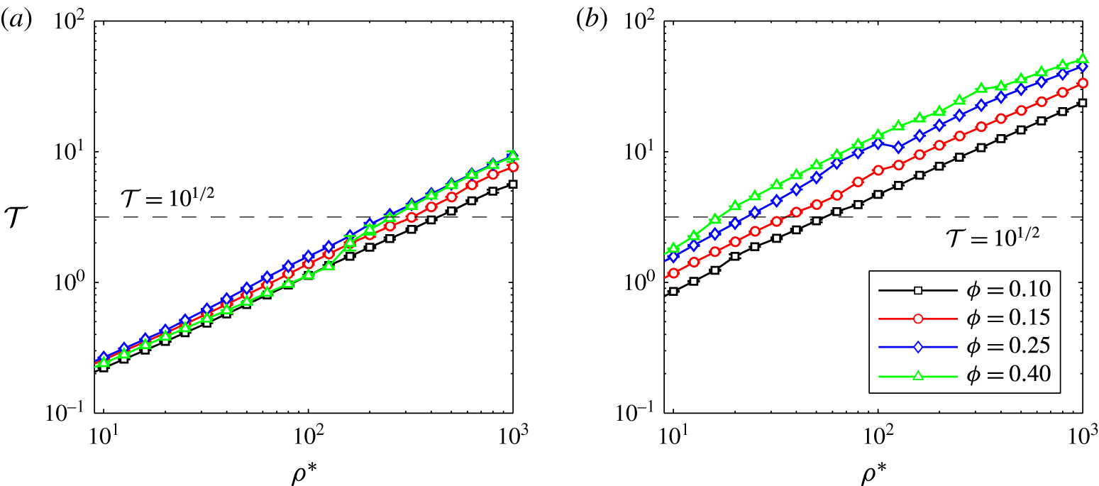
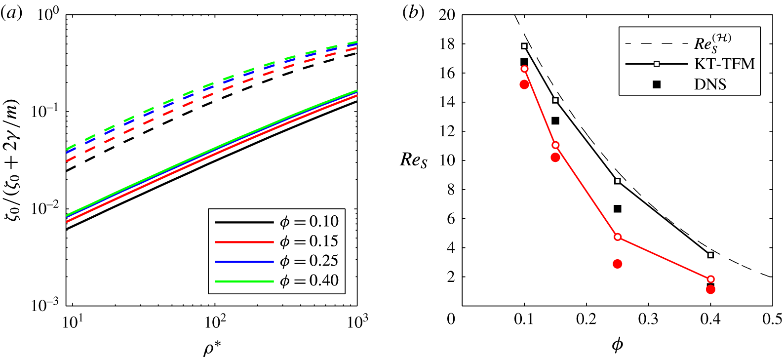
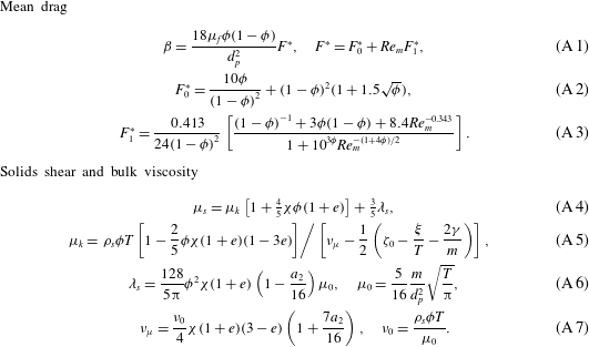
Figure 5 summarizes the calculation of
 ${\mathcal{T}}$
for the elastic conditions studied. The intersections of the
 ${\mathcal{T}}$
-curves with
 $10^{1/2}$
, i.e. the equality of (4.4), demarks a critical density ratio which is indicated by the vertical red lines in figures 6–9. As discussed below (§§ 4.2 and 4.3), the results indicate that this high-
 $St_{T}$
assumption (4.4) of the continuum theory is needed for accurate predictions.
Maximum normalized concentration difference in the KT-TFM simulations as a function of density ratio for
 $e=1$
and (a)
 $Ar=71$
and (b)
 $Ar=1432$
at mean concentrations of
 $\langle \unicode[STIX]{x1D719}\rangle =0.1$
(black), 0.15 (red), 0.25 (blue) and 0.40 (green). The thin dashed lines of similar colour show
 ${\mathcal{T}}$
in the homogeneous state.

4.2 Mean solids velocity
In this section we focus on mean solids velocity and make direct quantitative comparisons between the KT-TFM predictions and the DNS data. For the comparison, the continuum variable that is the solids velocity is Favre averaged. In the limit
 $\unicode[STIX]{x1D6E5}^{\ast }\rightarrow 0$
,
 $\unicode[STIX]{x1D719}$
becomes a phase indicator function and the Favre average becomes equivalent to a simple (discrete) particle average, consistent with the DNS results. Through a combination of volume, Favre and time averaging, equations (2.15)–(2.17), the space- and time-dependent data for an entire simulation can be reduced to a set of mean, scalar quantities for a given set of conditions (
 $Ar$
,
 $\unicode[STIX]{x1D70C}^{\ast }$
,
 $\langle \unicode[STIX]{x1D719}\rangle$
,
 $e$
). We present the mean sedimenting Reynolds number,
 $$\begin{eqnarray}Re_{S}=\frac{\unicode[STIX]{x1D70C}_{f}d_{p}}{\unicode[STIX]{x1D707}_{f}}|\overline{\langle \langle v_{s}\rangle \rangle }|,\end{eqnarray}$$
which measures the mean streamwise (vertical) velocity of the solids. Non-dimensionalization is required to compare the results of KT-TFM simulations performed in physical units with DNS simulations performed in lattice units. Here,
 $Re_{S}$
is preferred to
 $Re_{m}$
because the averaging is simpler; however, the two measurements are roughly similar. In fact, in the homogeneous state it can be shown that
 $Re_{S}^{({\mathcal{H}})}=Re_{m}^{({\mathcal{H}})}$
due to the specification
 $j_{y}^{({\mathcal{H}})}=0$
.
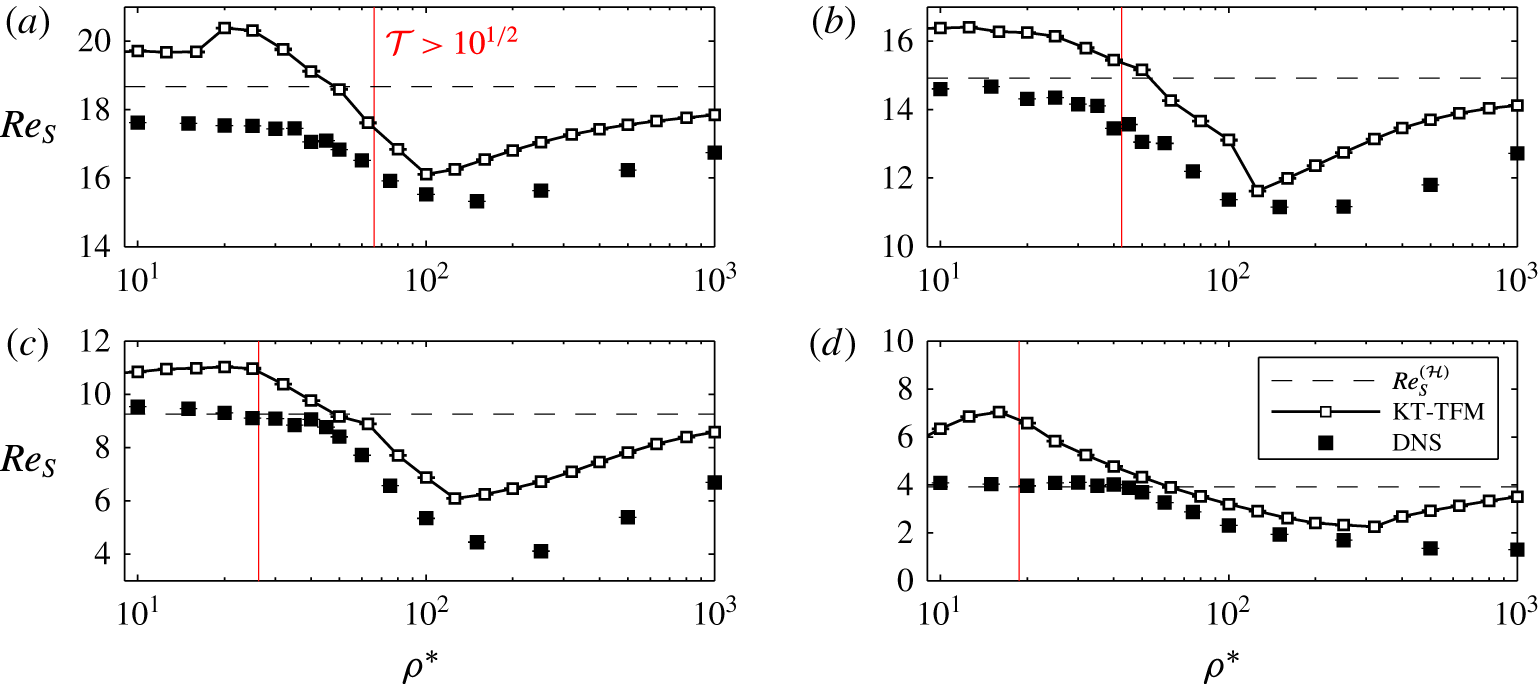
Figure 6 compares KT-TFM predictions of
 $Re_{S}$
to the DNS data as a function of
 $\unicode[STIX]{x1D70C}^{\ast }$
for
 $Ar=71$
,
 $e=1.0$
and the four mean concentrations:
 $\langle \unicode[STIX]{x1D719}\rangle =0.10$
, 0.15, 0.25 and 0.40. Each DNS data point represents an average of five replicate simulations with different initial conditions, although each simulation is run for a shorter time than the continuum simulations. The standard deviation of the five DNS replicates are shown as error bars in figure 6. In most cases, the error bars are too tight to extend above/below the data points representing the mean. The horizontal dashed lines show
 $Re_{S}^{({\mathcal{H}})}$
calculated from (2.12), which is independent of
 $\unicode[STIX]{x1D70C}^{\ast }$
for the drag law, equations (A 1)–(A 3), of Beetstra, van der Hoef & Kuipers (Reference Beetstra, van der Hoef and Kuipers2007) used here. The vertical red lines indicate the critical density ratio needed to uphold the high-
 $St_{T}$
(nearly Maxwellian) assumption of (4.4). The KT-TFM theory is expected to be valid to the right of the red line, i.e. at higher
 $\unicode[STIX]{x1D70C}^{\ast }$
. Generally, good agreement is observed in these regions, which appears to be a conservative estimate in some instances, especially at lower concentrations. Although the exact shape of the four KT-TFM
 $Re_{S}$
-curves in figure 6 are different, a similar trend is observed:
 $Re_{S}$
is largest at an intermediate density ratio (
 $\unicode[STIX]{x1D70C}^{\ast }\approx 100$
) and appears to decay at low and high density ratios. At lower density ratios,
 $Re_{S}$
decreases because the KT-TFM solution approaches a homogeneous state (
 $\unicode[STIX]{x0394}\unicode[STIX]{x1D719}_{max}\rightarrow 0$
in figure 1) which is most evident at higher concentrations as
 $Re_{S}$
coincides with
 $Re_{S}^{({\mathcal{H}})}$
over a range of
 $\unicode[STIX]{x1D70C}^{\ast }$
. The discrepancy between the DNS results and
 $Re_{S}^{({\mathcal{H}})}$
(determined from a DNS-based drag law) at low density ratio may be due to the specification of a fixed-bed-type drag law. Recently, Rubinstein et al. (Reference Rubinstein, Derksen and Sundaresan2016) postulated that a Wen & Yu (Reference Wen and Yu1966) type drag law is more appropriate for such low mean-flow Stokes number flows. Although the incorporation of such a mean-flow-Stokes-number-dependent drag law may also improve the KT-TFM predictions in this region, the most significant difference would be expected to occur outside of the intended range of validity, i.e. to the left of the red lines.
Comparison of KT-TFM predictions (thick lines) to DNS data (symbols) of the sedimenting Reynolds number for
 $Ar=71$
and (a)
 $\langle \unicode[STIX]{x1D719}\rangle =0.10$
, (b)
 $\langle \unicode[STIX]{x1D719}\rangle =0.15$
, (c)
 $\langle \unicode[STIX]{x1D719}\rangle =0.25$
and (d)
 $\langle \unicode[STIX]{x1D719}\rangle =0.40$
. Black dashed lines show homogeneous (stable) solutions,
 $Re_{S}^{({\mathcal{H}})}$
. Right-hand side of vertical red lines demarcates high-
 $St_{T}$
region of (4.4).

Conversely at large
 $\unicode[STIX]{x1D70C}^{\ast }$
, the suspension remains inhomogeneous (
 $\unicode[STIX]{x0394}\unicode[STIX]{x1D719}_{max}>0$
in figure 1) yet
 $Re_{S}$
decays to the point of
 $Re_{S}^{({\mathcal{H}})}$
and below, in some instances. A hindered sedimenting velocity, i.e.
 $Re_{S}<Re_{S}^{({\mathcal{H}})}$
, is a consequence of an increase in mean drag – a counterintuitive result since the clustering instability of gas–solid particle flow is most often associated with a mean drag reduction occasionally referred to as flow bypass, e.g. Agrawal et al. (Reference Agrawal, Loezos, Syamlal and Sundaresan2001), Li & Kwauk (Reference Li and Kwauk2001), Heynderickx et al. (Reference Heynderickx, Das, De Wilde and Marin2004), Beetstra, van der Hoef & Kuipers (Reference Beetstra, van der Hoef and Kuipers2006), Wang et al. (Reference Wang, Lu, Liu, Sheng, Xu and Gidaspow2011), Shah et al. (Reference Shah, Utikar, Tade, Evans and Pareek2013), Zhou et al. (Reference Zhou, Xiong, Wang, Wang, Ren and Ge2014) among others. Note that
 $Re_{S}<Re_{S}^{({\mathcal{H}})}$
at
 $\unicode[STIX]{x1D70C}^{\ast }\approx 1000$
is observed in the DNS data as well. The observed decay in
 $Re_{S}$
at high
 $\unicode[STIX]{x1D70C}^{\ast }$
is due to the change in flow structure discussed previously, namely the transition from the unsteady chaotic regime to the steady plug regime. For horizontal structure formed in the chaotic regime, the fluid has enough inertia to penetrate the plug and flow bypass is possible, although intermittent (see figure 2). In the steady (nonlinearly stable) plug regime, the plug structure is persistent and the fluid is forced to flow through the width-spanning, dense cluster (see figure 3). As the density ratio increases, the plug becomes more one-dimensional which causes more of the solids concentration to move from the funnel region into the horizontal plug region, further decreasing the sedimenting velocity. While the clustering structures observed here are a result of the small domain size, the accurate prediction of the counter-intuitive results displayed in figure 6 bodes well for the predictive capability of the GTSH KT-TFM, at least where it is expected to be valid (to the right of the vertical red line).
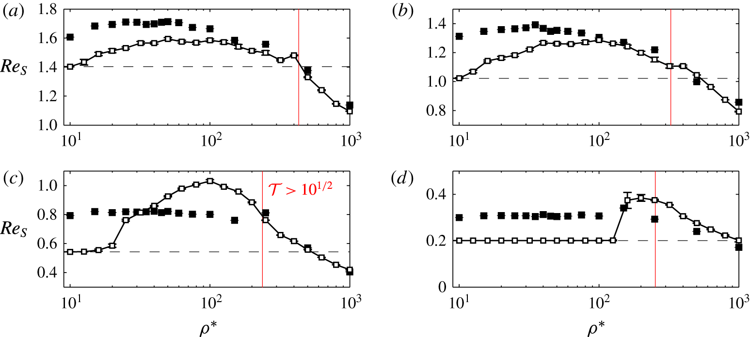
Comparison of KT-TFM predictions (thick lines) to DNS data (symbols) of the sedimenting Reynolds number for
 $Ar=1432$
and (a)
 $\langle \unicode[STIX]{x1D719}\rangle =0.10$
, (b)
 $\langle \unicode[STIX]{x1D719}\rangle =0.15$
, (c)
 $\langle \unicode[STIX]{x1D719}\rangle =0.25$
and (d)
 $\langle \unicode[STIX]{x1D719}\rangle =0.40$
. Black dashed lines show homogeneous (stable) solutions,
 $Re_{S}^{({\mathcal{H}})}$
. Right-hand side of vertical red lines demarcates high-
 $St_{T}$
region of (4.4).

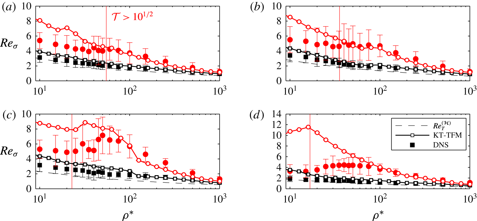
Figure 7 shows the same comparison as in figure 6 but at the higher
 $Ar=1432$
condition, which results in a wholesale increase of
 $Re_{S}$
by approximately one order of magnitude. As in figure 6, the red lines approximate where the high-
 $St_{T}$
condition (4.4) is valid, but are shifted to significantly lower density ratios compared to the
 $Ar=71$
case. Again, good agreement except for a slight over-prediction is generally seen where the theory is expected to be valid, and this agreement deteriorates to the left of the red line. The over-prediction of the DNS data by KT-TFM – even in the valid range – occurs at all concentrations, hinting that there may be a discrepancy between the mean drag law and the current set of DNS data. This discrepancy may be due, in part, to the increased uncertainty in the mean drag law at this higher Reynolds number, e.g. see comparisons in Tenneti, Garg & Subramaniam (Reference Tenneti, Garg and Subramaniam2011), Tang et al. (Reference Tang, Peters, Kuipers, Kriebitzsch and van der Hoef2015). Similar to the
 $Ar=71$
case, figure 7 shows that
 $Re_{S}$
decays with increasing
 $\unicode[STIX]{x1D70C}^{\ast }$
and a hindered mean sedimenting velocity,
 $Re_{S}<Re_{S}^{({\mathcal{H}})}$
, is observed in the KT-TFM predictions, consistent with the DNS data. However, two significant distinctions relative to the lower
 $Ar$
results (figure 6) can be seen: (i) the lowest density ratios are no longer small enough to observe the near-homogeneous state with the KT-TFM and (ii) the decay of
 $Re_{S}$
with
 $\unicode[STIX]{x1D70C}^{\ast }$
is not unbounded; at a given density ratio (in the vicinity of
 $\unicode[STIX]{x1D70C}^{\ast }\approx 200$
) the trend changes, rather abruptly in some instances, and
 $Re_{S}$
begins to increase. The latter is a new feature of higher
 $Ar$
and one that is captured remarkably well by the KT-TFM. The local minima in the sedimenting velocity curves of figure 7 coincide with the loss of the 2-D plug structure, i.e. transition in flow structure from that of figure 3 to that of figure 4. As the density ratio continues to increase, the peak concentration of the plug is reduced as the magnitude of the 1-D wave relaxes, leading to a reduction in the maximum drag experienced. Although the dilute regions are also less dilute, the strong nonlinearity in the concentration dependence of the drag law (A 1)–(A 3) causes an overall decrease in drag, causing the increase in
 $Re_{S}$
observed in figure 7. A few exploratory studies were carried out on a coarser grid to investigate the increasing
 $Re_{S}$
behaviour beyond
 $\unicode[STIX]{x1D70C}^{\ast }=1000$
. Up to
 $\unicode[STIX]{x1D70C}^{\ast }=100\,000$
,
 $Re_{S}$
does not cross the homogeneous solution again but asymptotes to it, i.e.
 $Re_{S}<Re_{S}^{({\mathcal{H}})}$
as
 $\unicode[STIX]{x1D70C}^{\ast }\rightarrow \infty$
.
4.3 Fluctuating solids velocity
In this section we move from mean to fluctuating statistics. Before jumping directly to a comparison with the DNS data, the KT-TFM variables will be reviewed, specifically how the continuum variables are defined from the probabilistic KT variables. The three variables used in the governing equations in table 1, concentration, mean velocity and granular temperature, are defined by
 $$\begin{eqnarray}\displaystyle & \displaystyle \unicode[STIX]{x1D719}={\mathcal{V}}_{p}\displaystyle \int f(\boldsymbol{x},\boldsymbol{v}_{p},t)\,\text{d}\boldsymbol{v}_{p}, & \displaystyle\end{eqnarray}$$
 $$\begin{eqnarray}\displaystyle & \displaystyle \boldsymbol{U}_{s}=\frac{{\mathcal{V}}_{p}}{\unicode[STIX]{x1D719}}\int \boldsymbol{v}_{p}f(\boldsymbol{x},\boldsymbol{v}_{p},t)\,\text{d}\boldsymbol{v}_{p}, & \displaystyle\end{eqnarray}$$
and
 $$\begin{eqnarray}T=\frac{1}{3}\frac{{\mathcal{V}}_{p}}{\unicode[STIX]{x1D719}}\int (\boldsymbol{v}_{p}-\boldsymbol{U}_{s})^{2}f(\boldsymbol{x},\boldsymbol{v}_{p},t)\,\text{d}\boldsymbol{v}_{p},\end{eqnarray}$$
respectively (Garzó et al.
Reference Garzó, Tenneti, Subramaniam and Hrenya2012). In (4.6)–(4.8),
 ${\mathcal{V}}_{p}$
is the particle volume,
 $\boldsymbol{v}_{p}=(u_{p},v_{p},w_{p})^{\text{T}}$
is the particle velocity and
 $f$
is the single-particle velocity distribution function. Similarly, the total (solids) kinetic energy can be defined by
 $$\begin{eqnarray}E_{s}=\frac{1}{2}\frac{{\mathcal{V}}_{p}}{\unicode[STIX]{x1D719}}\int \boldsymbol{v}_{p}^{2}f(\boldsymbol{x},\boldsymbol{v}_{p},t)\,\text{d}\boldsymbol{v}_{p}.\end{eqnarray}$$
The total kinetic energy is infrequently encountered in the literature because it is redundant, i.e. it can be equivalently determined by
 $$\begin{eqnarray}E_{s}={\textstyle \frac{1}{2}}(\boldsymbol{U}_{s}^{2}+3T).\end{eqnarray}$$
Although (4.10) could be directly compared with discrete particle data, it is more informative to introduce an approximation to decompose the kinetic energy into its directional components in order to study any anisotropy present in the system. By assuming that the (microscopic) fluctuating velocities are isotropic, i.e.
 $u_{p}u_{s}\approx v_{p}v_{s}\approx w_{p}w_{s}\approx T/3$
, equation (4.8) can be manipulated to give
 $$\begin{eqnarray}E_{s,x}={\textstyle \frac{1}{2}}(u_{s}^{2}+T),\quad E_{s,y}={\textstyle \frac{1}{2}}(v_{s}^{2}+T),\quad \text{and}\quad E_{s,z}={\textstyle \frac{1}{2}}(w_{s}^{2}+T).\end{eqnarray}$$
Now, considering again the analogy between a simple discrete particle average and a volume average with infinite resolution. Previously it was mentioned that the appropriate quantity to compare to the particle mean velocity (discrete particle, DNS) is the Favre-averaged velocity (continuum, KT-TFM). Likewise, the appropriate quantity to compare to the particle velocity variance is the difference between the Favre-averaged kinetic energy and the Favre-averaged velocity squared, a measure of the fluctuating kinetic energy. As before, the fluctuating kinetic energy is time averaged and non-dimensionalized into a Reynolds number:
 $$\begin{eqnarray}Re_{\unicode[STIX]{x1D70E},x}=\frac{\unicode[STIX]{x1D70C}_{f}d_{p}}{\unicode[STIX]{x1D707}_{f}}\overline{[\langle \langle u_{s}^{2}\rangle \rangle +\langle \langle T\rangle \rangle -\langle \langle u_{s}\rangle \rangle ^{2}]^{1/2}},\quad Re_{\unicode[STIX]{x1D70E},y}=\frac{\unicode[STIX]{x1D70C}_{f}d_{p}}{\unicode[STIX]{x1D707}_{f}}\overline{[\langle \langle v_{s}^{2}\rangle \rangle +\langle \langle T\rangle \rangle -\langle \langle v_{s}\rangle \rangle ^{2}]^{1/2}}.\end{eqnarray}$$
The total fluctuating kinetic energy is the sum of two contributions: (i) a modelled ‘microscopic’ component arising from the granular temperature,
 $\langle \langle T\rangle \rangle$
, and (ii) a resolved ‘macroscopic’ component arising from variations in the mean velocity,
 $\langle \langle u_{s}^{2}\rangle \rangle -\langle \langle u_{s}\rangle \rangle ^{2}$
. Moving forward, it is worthwhile to note that (4.12) is an approximate comparison due to the directional decomposition, although the assumption of isotropy only extends to the microscopic contribution.
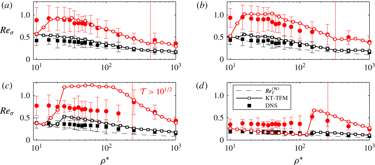
Comparison of KT-TFM predictions (thick lines) to DNS data (symbols) of the Reynolds number based on the standard deviation of the solids velocity in the
 $x$
- (black, squares) and
 $y$
-directions (red, circles) for
 $Ar=71$
and (a)
 $\langle \unicode[STIX]{x1D719}\rangle =0.10$
, (b)
 $\langle \unicode[STIX]{x1D719}\rangle =0.15$
, (c)
 $\langle \unicode[STIX]{x1D719}\rangle =0.25$
and (d)
 $\langle \unicode[STIX]{x1D719}\rangle =0.40$
. Black dashed lines show homogeneous (stable) solutions,
 $Re_{T}^{({\mathcal{H}})}$
. Right-hand side of vertical red lines demarcates high-
 $St_{T}$
region of (4.4).

Comparisons of
 $Re_{\unicode[STIX]{x1D70E}}$
between the DNS data and the KT-TFM simulations are provided in figures 8 and 9 for the elastic cases
 $Ar=71$
and 1432, respectively. Error bars of the DNS data again show the standard deviation of the five replicates, which are considerably larger here than in figures 6 and 7 since
 $Re_{\unicode[STIX]{x1D70E}}$
is based on second-order statistics (particle velocity variance). Both the streamwise,
 $Re_{\unicode[STIX]{x1D70E},y}$
(red circles), and transverse,
 $Re_{\unicode[STIX]{x1D70E},x}$
(black squares), directions are shown for comparison. In all cases, DNS and KT-TFM results are insensitive to the which transverse direction is considered, i.e.
 $Re_{\unicode[STIX]{x1D70E},x}\approx Re_{\unicode[STIX]{x1D70E},z}$
, and therefore only one is provided in figures 8 and 9 for clarity. The similarity of the statistics in the
 $x$
- and
 $z$
-directions is not surprising, given that the system is identical in both transverse directions. The homogeneous solution is also provided for comparison, which, unlike
 $Re_{S}$
, has a functional dependence on
 $\unicode[STIX]{x1D70C}^{\ast }$
. Since the homogeneous (stable) state is constant and uniform in space and time,
 $\langle \langle u_{s}^{2}\rangle \rangle =\langle \langle u_{s}\rangle \rangle ^{2}$
and
 $\langle \langle v_{s}^{2}\rangle \rangle =\langle \langle v_{s}\rangle \rangle ^{2}$
and, hence, (4.12) reduces to the thermal Reynolds number, i.e.
 $Re_{\unicode[STIX]{x1D70E}}^{({\mathcal{H}})}=Re_{T}^{({\mathcal{H}})}$
. As before, the vertical red lines represent the high-
 $St_{T}$
criterion of (4.4). Again, good agreement is generally observed where theory is expected to be valid and the agreement deteriorates moving to the left of the red line. Two notable exceptions are the comparisons at
 $Ar=71$
and
 $\langle \unicode[STIX]{x1D719}\rangle =0.10$
and 0.15 where good agreement is also observed to the left of the red line except at very low
 $\unicode[STIX]{x1D70C}^{\ast }$
where the KT-TFM becomes homogeneous; such agreement beyond the expected region of validity in these instances may be fortuitous. All cases show that the streamwise fluctuations (
 $y$
-direction) are significantly larger than the transverse fluctuations (
 $x$
- and
 $z$
-directions), which vary only slightly from
 $Re_{T}^{({\mathcal{H}})}$
, at least where good agreement with the DNS data is observed. The good agreement of the KT-TFM predictions of
 $Re_{\unicode[STIX]{x1D70E},y}$
and
 $Re_{\unicode[STIX]{x1D70E},x}$
with the DNS data supports the assumption of isotropic microscale fluctuations, i.e. the primary cause for the difference in magnitudes between
 $Re_{\unicode[STIX]{x1D70E},y}$
and
 $Re_{\unicode[STIX]{x1D70E},x}$
is due to fluctuating kinetic energy generated by macroscopic (resolved) variations in the mean flow rather than microscopic (modelled) granular temperature. Although these comparisons can only be considered approximate, the fluctuating kinetic energy is the greatest level of detail compared between DNS and highly resolved KT-TFM to date and the good agreement observed speaks to the accuracy of KT-TFM in predicting clustering.
Comparison of KT-TFM predictions (thick lines) to DNS data (symbols) of the Reynolds number based on the standard deviation of the solids velocity in the
 $x$
- (black, squares) and
 $y$
-directions (red, circles) for
 $Ar=1432$
and (a)
 $\langle \unicode[STIX]{x1D719}\rangle =0.10$
, (b)
 $\langle \unicode[STIX]{x1D719}\rangle =0.15$
, (c)
 $\langle \unicode[STIX]{x1D719}\rangle =0.25$
and (d)
 $\langle \unicode[STIX]{x1D719}\rangle =0.40$
. Black dashed lines show homogeneous (stable) solutions,
 $Re_{T}^{({\mathcal{H}})}$
. Right-hand side of vertical red lines demarcates high-
 $St_{T}$
region of (4.4).

Although attention here has been focused on the high-
 $St_{T}$
region, where the KT-TFM predictions are expected to be valid, one consistent trend in the KT-TFM data in the lower-
 $St_{T}$
region is worth noting. Except for where the KT-TFM is at or approaching the homogeneous condition, i.e.
 $Re_{S}\rightarrow Re_{S}^{({\mathcal{H}})}$
and
 $Re_{\unicode[STIX]{x1D70E}}\rightarrow Re_{T}^{({\mathcal{H}})}$
, there is a direct correlation between the over-prediction of
 $Re_{S}$
and
 $Re_{\unicode[STIX]{x1D70E}}$
. Although fluctuating kinetic energy is the sum of mean flow and granular temperature components, deviations in
 $T$
from
 $T^{({\mathcal{H}})}$
are predominantly due to viscous heating,
 $\unicode[STIX]{x1D748}_{s}\boldsymbol{ : }\unicode[STIX]{x1D735}\boldsymbol{U}_{s}$
in (2.5), which is an inherently inhomogeneous term (if the system is near the homogeneous condition,
 $U_{s}$
is uniform and there is no viscous heating). Therefore,
 $Re_{\unicode[STIX]{x1D70E}}$
and in particular its deviation from
 $Re_{T}^{({\mathcal{H}})}$
can serve as an indication of the degree of inhomogeneity in the system. Consequently, the correlation between the over-prediction of
 $Re_{\unicode[STIX]{x1D70E}}$
and
 $Re_{S}$
suggests that the KT-TFM is over-predicting the degree of segregation (inhomogeneity), or ‘over-clustering’, which is producing larger fluctuating energy levels via larger variations in mean flow and consequently leading to an increased mean velocity via enhanced flow bypass. The enhanced segregation of the KT-TFM has been previously observed by Desjardins, Fox & Villedieu (Reference Desjardins, Fox and Villedieu2008) in the context of preferential concentration in frozen fluid-phase turbulence. Furthermore, it has been suggested that over-segregation of KT-TFM predictions is not only limited to the dilute, low mean-flow Stokes number regions (Passalacqua et al.
Reference Passalacqua, Fox, Garg and Subramaniam2010). We conclude by noting that while the issue of over-segregation may contribute to disagreement between the KT-TFM predictions and the DNS data near the validity criteria (red line), good agreement is generally observed moving away from the estimated point of critical validity.
4.4 Regime boundary
As evidenced by three specific instances in § 3, the qualitative agreement between the KT-TFM and DNS is quite remarkable. Here, we attempt to compare the structure of the suspension in a more quantitative manner by calculating the transition between the chaotic and (2-D) plug regimes which was observed at both high and low
 $Ar$
numbers and all concentrations considered here. The transition will be characterized by a critical density ratio,
 $\unicode[STIX]{x1D70C}_{c}^{\ast }$
, for both KT-TFM and DNS.
As mentioned in § 3, the transition between the chaotic and plug regimes is gradual, which makes the identification of a single transition value, i.e.
 $\unicode[STIX]{x1D70C}_{c}^{\ast }$
, complicated. Figure 2 shows that plug-like structures form even in the chaotic region, at least temporarily. However, the two regimes may be distinguished by whether or not the fluid has enough inertia to break up the plugs. Therefore,
 $\unicode[STIX]{x1D70C}_{c}^{\ast }$
may be equivalently identified as the density ratio at which plugs persist (rather than simply exist).
In DNS, persistent plugs are identified using the structure factor. The structure factor is the Fourier transform of the particle pair distribution and can be calculated using
 $$\begin{eqnarray}S(\unicode[STIX]{x1D73F})=\frac{1}{N}\mathop{\sum }_{i}\mathop{\sum }_{j}\text{e}^{-\unicode[STIX]{x1D73F}\boldsymbol{\cdot }\boldsymbol{r}_{ij}\sqrt{-1}}.\end{eqnarray}$$
Here,
 $\boldsymbol{r}_{ij}$
is the vector from the centre of particle
 $i$
to particle
 $j$
, and
 $\unicode[STIX]{x1D73F}$
is the wave vector. Excess or deficit of
 $S(\unicode[STIX]{x1D73F})$
from its equilibrium value of unity is an indication that the spatial distribution of particles has a Fourier component in the direction of
 $\unicode[STIX]{x1D73F}$
with wavelength
 $2\unicode[STIX]{x03C0}|\unicode[STIX]{x1D73F}|^{-1}$
. In a periodic domain, the number of structures must be a positive integer. The first, second, and third structure factors along the direction of sedimentation are therefore given by
 $$\begin{eqnarray}S_{y}^{\{k\}}=\frac{1}{N}\mathop{\sum }_{i}\mathop{\sum }_{j}\text{e}^{-(2k\unicode[STIX]{x03C0}/L_{y}^{\ast })(y_{i}^{\ast }-y_{j}^{\ast })\sqrt{-1}},\end{eqnarray}$$
where
 $k=1$
, 2 and 3, respectively. Persistent plugs are identified by the first, second or third structure factors attaining a value greater than 25 for 50 % of the simulation time. Figure 10 shows the evolution of
 $S_{y}^{\{k\}}$
, obtained from a system with
 $Ar=1432$
,
 $\unicode[STIX]{x1D70C}^{\ast }=25$
,
 $\langle \unicode[STIX]{x1D719}\rangle =0.25$
and
 $e=1.0$
. At time A, the highest structure factor was approximately 8, and the system only showed a slight heterogeneity that cannot be clearly distinguished from statistical fluctuations. At time B, the second structure factor reached 17, and heterogeneity started to become noticeable. After time B, the heterogeneity continues to increase and at time C two horizontal clusters can be clearly identified when the second structure factor has a value of 36. As this simulation has strong clusters for more than 50 % of the time, it is identified as one with persistent plugs.
The graph on the far right shows the evolution of the first three structure factors in the
 $y$
-direction for a simulation with
 $Ar=1432$
,
 $\unicode[STIX]{x1D70C}^{\ast }=25$
,
 $\langle \unicode[STIX]{x1D719}\rangle =0.25$
and
 $e=1.0$
. In this case, the second structure factor (dotted line) increases significantly as the simulation progresses. Visualization of distributions of particle centres (left three graphs) at three different times (A, B and C) shows heterogeneities that grow with time, and specifically the two-cluster structure at time C.

The structure factor is calculated based on particle locations and is therefore not directly applicable to continuum (KT-TFM) results. A successful regime indicator was found by examining the temporal signatures, which provide a measure of the dynamics of the system rather than the spatial structure of the system. Namely, the 2-D and 1-D plug regimes manifest as travelling wave limit cycles which are cyclical and regular, while the chaotic regime is dynamic and irregular. The two types of system dynamics are differentiated with a type of auto-correlation. First, the near-homogeneous cases are removed by excluding cases with
 $\unicode[STIX]{x0394}\unicode[STIX]{x1D719}_{max}<0.5$
. With the remaining inhomogeneous cases, the solids concentration field is decomposed into
 $N_{xyz}=N_{x}\times N_{y}\times N_{z}$
time signals denoted
 $\unicode[STIX]{x1D719}_{ijk}(t^{\ast })=\unicode[STIX]{x1D719}(x^{\ast }=x_{i}^{\ast },y^{\ast }=y_{j}^{\ast },z^{\ast }=z_{k}^{\ast },t^{\ast })$
, where
 $x_{i}^{\ast }$
,
 $y_{j}^{\ast }$
and
 $z_{k}^{\ast }$
are the
 $N_{xyz}$
discrete grid locations. Only the time in the averaging window,
 $[t_{1}^{\ast },t_{2}^{\ast }]$
, is considered. In the middle of each
 $\unicode[STIX]{x1D719}_{ijk}(t^{\ast })$
string, a time unit sample of length
 $\unicode[STIX]{x1D6FF}t\ast =200$
and 50 for
 $Ar=71$
and 1432, respectively, is selected. The sample is cross-correlated with the entire
 $\unicode[STIX]{x1D719}_{ijk}(t^{\ast })$
signal and by moving the sample in time by
 $\pm n\unicode[STIX]{x1D6E5}_{t}^{\ast }$
, where
 $n$
is a positive integer, The procedure is terminated when the sample reaches the beginning and end of the full signal. The
 $N_{xyz}$
temporal cross-correlations are then averaged over all spatial locations. When the sample is compared with itself, i.e. the auto-correlation at
 $n=0$
, the averaged cross-correlation is unity. As the sample moved to the left or right (forward or backward in time) the averaged cross-correlation decays. If the signal is perfectly cyclic – indicative of an exact travelling wave limit cycle – the cross-correlation will increase to unity again at secondary peaks indicating an exact correlation in the signals. The averaged cross-correlation will remain near zero if the two signals show no correlation (similarity) whatsoever. A simulation is considered to be in a plug-flow regime if a secondary peak (i.e. outside of the auto-correlation window) of the averaged cross-correlation attains a value of
 $2/3$
. Conversely, a simulation is considered to be in the chaotic regime if no secondary peak attains a value of
 $1/3$
(i.e. all secondary peaks
 ${<}1/3$
). This treatment will yield a range of
 $\unicode[STIX]{x1D70C}_{c}^{\ast }$
rather than a single value, which is representative of the smooth transition between the chaotic and plug regimes that
 $\unicode[STIX]{x1D70C}_{c}^{\ast }$
is meant to represent. The two criteria signifying the transition region between chaotic and plug regimes are represented as upper and lower error bars centred about their geometric mean.
Comparison of continuum predictions (thick lines with small, open symbols) to DNS data (filled symbols) of the critical density ratio for the transition of dynamic to plug-flow patterns at
 $Ar=71$
(black squares) and
 $Ar=1432$
(blue circles). The KT-TFM points show the geometric mean of the criteria for chaotic and plug regimes which are indicated by the lower and upper error bars, respectively. Dashed red and green lines indicate high-
 $St_{T}$
criteria of (4.4) for
 $Ar=71$
and 1432, respectively.

A comparison of the chaotic-to-plug transition criteria determined from the DNS and KT-TFM simulations is provided in figure 11. Except at the highest concentration,
 $\langle \unicode[STIX]{x1D719}\rangle =0.40$
, the comparisons are very favourable. It should be pointed out that the seemingly good agreement for
 $\langle \unicode[STIX]{x1D719}\rangle =0.40$
at
 $Ar=71$
is apparently fortuitous as the error bar separates a single pair of simulations which, unlike all other cases, transition directly from homogeneous to plug, skipping the chaotic regime entirely. It should also be mentioned that most cases fall just below the required thermal Stokes number criterion which may be responsible for the discrepancy. However, the good agreement in figure 11 is further evidence that the qualitative similarities between KT-TFM and DNS extend beyond the three select cases observed previously in § 3.
4.5 Knudsen number analysis
Although it has been demonstrated that the breakdown of the high-
 $St_{T}$
condition can explain the poor agreement between KT-TFM predictions and the DNS data at low density ratios, it is worthwhile to analyse another assumption used in the derivation of the KT-TFM: the low Knudsen number assumption. Recall that this assumption stems from the Chapman–Enskog expansion about a small parameter, namely the Knudsen number defined as
 $Kn\equiv \ell /L$
, where
 $\ell$
is the mean free path defined previously in § 4.1 and
 $L$
is a macroscopic length scale characterizing the local gradient, i.e.
 $L$
is small for large gradients and vice versa. Accordingly, the low-
 $Kn$
assumption is also referred to as the ‘small gradient’ assumption. A priori, this assumption appears at odds with the presence of clustering instabilities, since a relatively large concentration gradient is present normal to the cluster interface. This question motivates the subsequent analysis.
Following a previous work (Mitrano et al.
Reference Mitrano, Zenk, Benyahia, Galvin, Dahl and Hrenya2014), we take
 $L$
to be the length at which a variable of interest changes by 20 %, or
 $L_{f}=0.2|f|/|\unicode[STIX]{x1D735}f|$
, where
 $f$
is a variable of interest. Here, we consider the solids concentration, the vertical component of solids velocity and the granular temperature, i.e.
 $f=\unicode[STIX]{x1D719}$
,
 $v_{s}$
and
 $T$
. Special care is taken with the solids velocity. In the current system, the
 $v_{s}$
is only defined relative to the frame of reference. Hence,
 $Kn_{v}$
should be normalized with the thermal speed,
 $c$
, in order to eliminate the possibility of calculating a large value
 $Kn$
simply due to
 $v_{s}$
becoming (locally) null (Garzó & Santos Reference Garzó and Santos2003). The three Knudsen numbers of interest are then:
 $$\begin{eqnarray}Kn_{\unicode[STIX]{x1D719}}=\frac{5}{6\sqrt{2}}\frac{|\unicode[STIX]{x1D735}^{\ast }\unicode[STIX]{x1D719}|}{\unicode[STIX]{x1D719}^{2}\unicode[STIX]{x1D712}},\quad Kn_{v}=\frac{5}{12}\frac{|\unicode[STIX]{x1D735}^{\ast }v_{s}|}{\unicode[STIX]{x1D719}\unicode[STIX]{x1D712}\sqrt{T}},\quad \text{and}\quad Kn_{T}=\frac{5}{6\sqrt{2}}\frac{|\unicode[STIX]{x1D735}^{\ast }T|}{\unicode[STIX]{x1D719}\unicode[STIX]{x1D712}T},\end{eqnarray}$$
where
 $\unicode[STIX]{x1D735}^{\ast }$
is the gradient operator non-dimensionalized by particle diameter.
Instantaneous Knudsen numbers in a KT-TFM simulation at
 $Ar=71$
,
 $\langle \unicode[STIX]{x1D719}\rangle =0.15$
, and
 $\unicode[STIX]{x1D70C}^{\ast }=100$
and
 $e=1.0$
. A slice in the
 $xy$
-plane shows contours of (a)
 $Kn_{\unicode[STIX]{x1D719}}$
, (b)
 $Kn_{v}$
and (c)
 $Kn_{T}$
. The cumulative distribution function of each is provided in (d) considering the entire domain.

A typical example of the three Knudsen numbers defined by (4.15) is shown in figure 12 at a particular instant in a fully developed, statistically steady state. The contour plots and the cumulative distribution functions (CDF) all use a logarithmic scale. It is observed that all three Knudsen numbers span several orders of magnitude from approximately
 $O(10^{-2})$
to
 $O(10^{2})$
. Hence, calculating a simple
 $Kn$
mean value would be misleading, tending to skew the results to very large
 $Kn$
values. To avoid such bias, the ‘reverse’ analysis is performed: rather than seeing if the mean values exceed a given criterion, we seek to find what percentage of the domain exceeds the specified criterion. Similar to (4.4),
 $Kn$
is assumed to be sufficiently small if it is less than a negative half order of magnitude, i.e.
 $Kn<10^{-1/2}$
. For example, at the time shown in figure 12 approximately 80 % of the domain is violating the small-
 $Kn_{\unicode[STIX]{x1D719}}$
assumption, almost 90 % of the domain is violating the small-
 $Kn_{T}$
assumption, and nearly the entire domain is violating the small-
 $Kn_{v}$
assumption.
Time-averaged values of the percentage of the KT-TFM simulation domain with
 $Kn\geqslant 10^{-1/2}$
for
 $Ar=71$
and
 $\langle \unicode[STIX]{x1D719}\rangle =$
(a) 0.10, (b) 0.15, (c) 0.25 and (d) 0.40.
 $Kn_{\unicode[STIX]{x1D719}}$
,
 $Kn_{v}$
and
 $Kn_{T}$
are indicated by black, red and blue lines with open square, circle and diamond symbols, respectively.

Time-averaged values of the percentage of the KT-TFM simulation domain with
 $Kn\geqslant 10^{-1/2}$
for
 $Ar=1432$
and
 $\langle \unicode[STIX]{x1D719}\rangle =$
(a) 0.10, (b) 0.15, (c) 0.25 and (d) 0.40.
 $Kn_{\unicode[STIX]{x1D719}}$
,
 $Kn_{v}$
and
 $Kn_{T}$
are indicated by black, red and blue lines with square, circle and diamond symbols, respectively.

The percentage of the domain that violates the small-
 $Kn$
assumption, i.e. fractional region where
 $Kn\geqslant 10^{-1/2}$
, is time averaged and presented in figures 13 and 14 for the elastic cases
 $Ar=71$
and 1432, respectively. Two trends are readily apparent: (i) large portions of the domain are violating the low-
 $Kn$
assumption for all three variables of interest at both
 $Ar$
conditions and all mean concentrations considered and (ii) the velocity Knudsen number is almost always the largest of the three. The latter appears to be a result of the concentration field being out of phase with the solids velocity gradient, unlike the concentration and temperature gradients. In other words, where the concentration field exhibits a local minima, the gradients of concentration and temperature are also small and the two effects tend to counteract each other. The velocity gradients, on the other, are not typically small near concentration minima producing larger
 $Kn_{v}$
relative to
 $Kn_{\unicode[STIX]{x1D719}}$
and
 $Kn_{T}$
. At low
 $\unicode[STIX]{x1D70C}^{\ast }$
for
 $Ar=71$
, where some of the largest discrepancy between the KT-TFM and DNS results was observed due to violation of the high-
 $St_{T}$
assumption, all three Knudsen numbers are very small due to the near-homogeneous condition of the KT-TFM simulations. Conversely, in some regions where good agreement with DNS data was noted (high-
 $St_{T}$
regions), wholesale violations of the small-
 $Kn$
assumption are observed. The results of this analysis indicate that the small-
 $Kn$
assumption is not the culprit for the breakdown in the agreement with the DNS data, unlike the high-
 $St_{T}$
assumption. It is worthwhile to note that a similar observation (significant violation of
 $Kn$
assumption despite good agreement) was also reported in a previous work for the onset of clustering in the granular HCS (Mitrano et al.
Reference Mitrano, Zenk, Benyahia, Galvin, Dahl and Hrenya2014) where clustering was caused by particle inelasticity alone. The ability of the KT-TFM to perform well outside of its intended
 $Kn$
-range of validity is reminiscent of molecular gases, i.e. Navier–Stokes, and is very fortunate as higher-order theories such as linear-Burnett, Burnett, super-Burnett, etc. are unwieldy, particularly for engineering applications of particulate flows. Alternatively, moments of the starting kinetic equation can be solved directly, though unlike the Chapman Enskog method, such numerical solutions do not result in analytical expressions for the constitutive relations; see, for example, Desjardins et al. (Reference Desjardins, Fox and Villedieu2008).
4.6 Effect of inelasticity
All of the results presented thus far have been elastic, i.e.
 $e=1$
. Inelastic simulations, both DNS and KT-TFM, were also carried out for all cases with
 $e=0.9$
. For the sake of brevity, the results are not presented here since inelasticity did not have a significant impact on the systems examined. While
 $e$
has a widespread effect on the KT-TFM governing equations, its impact on the dissipation of granular temperature through the zeroth-order cooling rate,
 $\unicode[STIX]{x1D701}_{0}$
, see (A 21), may be the most important due to the role of granular temperature dissipation as a clustering mechanism (Fullmer & Hrenya Reference Fullmer and Hrenya2017b
). The contribution of inelasticity to the total dissipation (inelastic collisions
 $+$
thermal drag) is quantified in figure 15 for the homogeneous state. It is seen that inelasticity plays a relatively minor role in the total dissipation for the lower
 $Ar=71$
case throughout the
 $\unicode[STIX]{x1D70C}^{\ast }$
range. Only at
 $Ar=1432$
and the highest density ratios does inelasticity contribute at a similar level to the total dissipation as the thermal drag – which is also the only region where noticeable differences with the elastic simulations were observed.
(a) Ratio of thermal drag to total granular temperature dissipation (inelastic collisions
 $+$
thermal drag) for
 $\langle \unicode[STIX]{x1D719}\rangle =0.10$
(black), 0.15 (red), 0.25 (blue) and 0.40 (green) and
 $Ar=71$
(lower, solid lines) and
 $Ar=1432$
(upper, dashed lines). (b) Sedimenting Reynolds number at
 $Ar=1432$
,
 $\unicode[STIX]{x1D70C}^{\ast }=1000$
and
 $e=1.0$
(black) or
 $e=0.9$
(red) from DNS (symbols) and KT-TFM (thick lines) simulations. Dashed line show homogeneous (stable) solution,
 $Re_{S}^{({\mathcal{H}})}$
.

Figure 15 also shows the effect of inelasticity on the sedimenting Reynolds number for the case most sensitive to
 $e$
, i.e.
 $Ar=1432$
and
 $\unicode[STIX]{x1D70C}^{\ast }=1000$
. The DNS data show a decrease in
 $Re_{S}$
for all concentrations – a trend that is matched in the KT-TFM predictions. Quantitatively, the inelastic KT-TFM predictions agree with the DNS data slightly more favourably than the elastic results. The decrease of
 $Re_{S}$
has come about by a change in structure that can be best understood when viewed in terms of the most important consequence of particle inelasticity: a source of clustering. In general, clustering in gas–solid flows is induced by either a difference in mean relative motion and/or the dissipation of granular temperature (Fullmer & Hrenya Reference Fullmer and Hrenya2017b
). Due to thermal drag (which leads to a dissipation of granular temperature), both sources of clustering are present in the elastic cases, so the inclusion of particle inelasticity does not change the stability pattern of the system appreciably. However, the inelastic cases always have more dissipation and are therefore more unstable than the elastic cases which has the effect of moving the flow pattern regime boundaries to lower density ratios. One can imagine that the
 $Re_{S}$
curves of figure 7 have been shifted to the left (but a non-uniform shift due to the diminishing impact of
 $\unicode[STIX]{x1D701}_{0}$
with decreasing
 $\unicode[STIX]{x1D70C}^{\ast }$
shown in figure 15
a). Therefore, while the flow structure for all cases presented in figure 15(b) are in the 1-D plug regime, the amplitude of the plug is still larger in the inelastic cases. In closing, it is worth noting that the minor impact of inelasticity observed here should not be extrapolated to highly inelastic conditions or, perhaps more importantly, to higher mean-flow Stokes number conditions (i.e. higher
 $Ar$
and/or
 $\unicode[STIX]{x1D70C}^{\ast }$
).
5 Concluding remarks
In this work, a fully periodic suspension of solid particles in a state of sedimentation (or fluidization) is studied with direct numerical simulation and a two-fluid (continuum) model derived from the kinetic theory approach (KT-TFM). The study considered two Archimedes numbers (which determines the system mean-flow Reynolds number),
 $Ar=71$
and 1432; four mean concentrations,
 $\langle \unicode[STIX]{x1D719}\rangle =0.10$
, 0.15, 0.25 and 0.40; a wide range of density ratios,
 $\unicode[STIX]{x1D70C}^{\ast }=10{-}1000$
; and two restitution coefficients
 $e=1.0$
and 0.9, although the focus was primarily on the elastic results. The novelty of such a study is not simply the KT-TFM results themselves, but a detailed comparison to data generated via DNS throughout an extensive phase space of conditions, producing a variety of instability patterns. KT-TFMs are widely used to simulate gas–solid flows and are especially relevant to the construction of, and in many cases the closure of, filtered TFMs that are applied to engineering and industrial applications. Though a large number of studies exist with KT-TFMs, previous assessments on their quantitative accuracy in the presence of clusters has been scarce.
Since the computational expense associated with DNS is considerable, the system size considered here is very small, no more than 35 particle diameters in the longest (vertical) dimension. Therefore, when clustering occurs it forms a significantly different structure than observed in large domains, e.g. (see Capecelatro et al.
Reference Capecelatro, Desjardins and Fox2015; Fullmer & Hrenya Reference Fullmer and Hrenya2016). A direct investigation of the flow patterns with instantaneous snapshots revealed three regimes of inhomogeneous (clustered) sedimentation: chaotic, 2-D plugs and 1-D plugs. All three regimes are also observed in the DNS data. The qualitative agreement of the flow structure between the KT-TFM and DNS is remarkable, particularly given the amount of behaviours observed and the violation of the small
 $Kn$
assumption.
Quantitative comparisons of the mean and fluctuating solids velocities show mixed results. The largest discrepancies generally appear at low density ratios while good agreement is observed at intermediate and high density ratios. By evaluating the key assumptions of the KT-TFM derivation, the significant discrepancy observed in the KT-TFM results was traced to the ratio of viscous-to-collisional time scales, equation (4.3), or equivalently the thermal Stokes number. In particular, an assumption of the KT-TFM that the single-particle velocity distribution function is nearly Maxwellian as a result of particle–particle collisions breaks down if the viscous relaxation time of the fluid approaches the mean time between successive collisions of the particles (i.e. low thermal Stokes numbers). A criterion was established (4.4) to approximate where the collision dominated assumption is upheld. By and large, it is shown that the poor and good agreement between the KT-TFM results and DNS data is observed in regions where this condition is violated or upheld, respectively. Moreover, a quantitative assessment of the observed flow regimes was undertaken by calculating a critical density ratio,
 $\unicode[STIX]{x1D70C}_{c}^{\ast }$
, demarcating the transition from chaotic to plug regimes. Comparisons of
 $\unicode[STIX]{x1D70C}_{c}^{\ast }$
are quite favourable, especially at the three lower mean concentrations.
Another important non-dimensional number associated with the underlying assumptions of the KT derivation, the Knudsen number,
 $Kn$
, was also studied. In the context of the Chapman–Enskog expansion,
 $Kn$
characterizes strength of spatial gradients relative to the microscopic length scale (particle mean free path). Unlike the time scale ratio, violation of the small-
 $Kn$
assumption did not show a strong correlation with the breakdown in the agreement of the KT-TFM predictions with the DNS data. In fact, large values of
 $Kn$
over a significant portion of the domain is observed where the KT-TFM predictions were quite good. Along with the previous work of Mitrano et al. (Reference Mitrano, Zenk, Benyahia, Galvin, Dahl and Hrenya2014), which studied granular flow in the HCS (i.e. only onset of clustering), this work adds to a growing body of work indicating that, like molecular fluids, Navier–Stokes-order theories may be applied outside of their intended range of Knudsen number validity. It is very fortunate for continuum modelling that the small-
 $Kn$
assumption may be relaxed, as extending the Navier–Stokes order theory considered here to higher order, e.g. Burnett order, quickly becomes intractable. The analysis of the non-dimensional numbers shows that some assumptions of the KT derivation may be relaxed, while others are rather strict. Furthermore, the insensitivity of the small-
 $Kn$
assumption suggests that perhaps even simpler models may be applied with minimal loss of accuracy. Future studies aimed at determining essential elements of the full Navier–Stokes-order theory for high-
 $St_{T}$
fluidization would be a welcome practical result for the further development of coarse-grained models (e.g. filtered or RANS KT-TFMs).
Unlike previous works which focused largely on qualitative comparisons, the present study quantitatively compares KT-TFM predictions directly to new DNS data of fully periodic gas–solid flows. In general, the assessment shows that a highly resolved KT-TFM is able to predict a domain-constrained clustering instability reasonably well at high Stokes numbers a welcome result for those using filtered TFMs derived from KT-TFMs which may have assumed this implicitly. Any realistic application, however, cannot be considered fully periodic. It is well known that in industrial and engineering applications, clustering is not spatially uniform, see e.g. Chew et al. (Reference Chew, Hays, Findlay, Knowlton, Karri, Cocco and Hrenya2012). Future studies assessing the predictive accuracy of KT-TFMs in wall-bounded fluidization should be performed.
Acknowledgements
The authors would like to thank V. Garzó, S. Subramaniam and S. Tenneti for insightful discussions on the GTSH theory and to S. Benyahia and J. E. Galvin for insightful discussions on the numerical implementation in MFiX. W.D.F. and C.M.H. would like to acknowledge funding from the National Science Foundation grant CBET-1236157. G.L. and X.Y. are grateful for funding from the National Science Foundation grant CBET-1236490. G.L. would also like to acknowledge funding from the National Science Foundation of China grant 51106039.
Supplementary movies
Supplementary movies are available at https://doi.org/10.1017/jfm.2017.295.
Appendix A
Momentum closure of the GTSH KT-TFM.
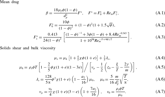
Thermal closure of the GTSH KT-TFM.
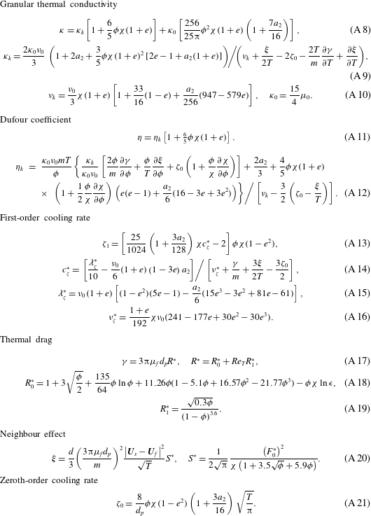
Ancillary definitions of the GTSH KT-TFM.
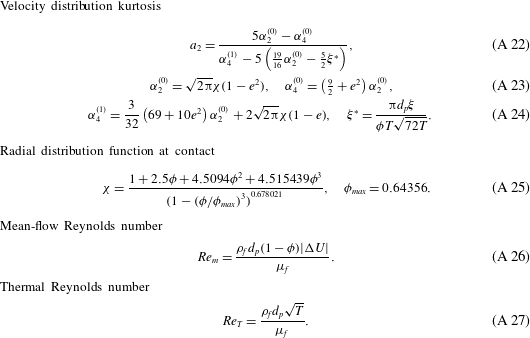
This appendix provides the remaining relations needed to fully specify the GTSH KT-TFM. For convenience, the additional closure relations have been split into solids-phase momentum terms in table 3, granular temperature terms in table 4 and other supporting definitions in table 5. Additionally, we highlight here a few minor differences between the model outlined in tables 1 and 3–5 and the original theory (Garzó et al.
Reference Garzó, Tenneti, Subramaniam and Hrenya2012). The DNS-based mean drag model of Beetstra et al. (Reference Beetstra, van der Hoef and Kuipers2007) is selected, equation (A 1) for the simulations herein as it is applicable to both low and intermediate mean-flow Reynolds numbers, equation (A 26), and was obtained from the same lattice Boltzmann code (SUSP3D) used in this study. It should be noted that
 $\unicode[STIX]{x1D6FD}$
represents only the steady drag component of the generalized interfacial momentum transfer force (Ishii & Hibiki Reference Ishii and Hibiki2006). Contributions from virtual (added) mass, lift, rotational, Basset, Faxèn, turbulent dispersion and wall forces, among others (Drew & Passman Reference Drew and Passman1999), have been neglected. Although the reduction of the generalized interfacial momentum transfer force to the steady drag force is common practice for gas–solid flows (Jackson Reference Jackson2000), this work does consider a wide range of conditions where this approximation may be questioned, particularly at low density ratios. Furthermore, even the definitions of the non-dimensional Stokes numbers would be affected by the inclusion of the virtual mass force, specifically by the inclusion of a fluid mass in the viscous relaxation time, equation (4.2). However, as such an inclusion results in at most a 3 % difference in the KT-TFM validity criteria used throughout this work, in which there is some degree of ambiguity to begin with see discussion around (4.3)–(4.4); accordingly, we feel that this assumption has minimal impact on the results reported herein. Further, we note that in general (2.3) should include a term related to the gas-phase stress tensor which has been neglected here. For flows with low density ratios this term may become more important. However, for the conditions considered herein, the homogeneous solids viscosity is strictly larger than the gas viscosity.
In the granular energy equation, (2.5), the thermal drag model of Wylie, Koch & Ladd (Reference Wylie, Koch and Ladd2003) is used, equation (A 17), which represents a first order in
 $Re_{T}$
extension to the model of Koch & Sangani (Reference Koch and Sangani1999), where
 $Re_{T}$
is the is the thermal Reynolds number defined by (A 27). The expression of (A 19) was re-fit to the original DNS data and enforced to have the proper limiting form
 $R_{1}^{\ast }(\unicode[STIX]{x1D719}\rightarrow 0)\rightarrow 0$
. This adjustment was found to be necessary to prevent the thermal conductivity, equation (A 8), from becoming negative in very dilute regions.
Two practical adjustments to the theory have been made to avoid ‘over-packing’, i.e. predicting solids concentrations above a physically realistic limit. First, the radial distribution function of Carnahan & Starling (Reference Carnahan and Starling1969) is replaced here with that of Ma & Ahmadi (Reference Ma and Ahmadi1988), equation (A 25). The two radial distribution functions are very similar at low to intermediate concentrations, though only the latter is applicable in the dense regime near the random close-packed limit,
 $\unicode[STIX]{x1D719}_{max}$
. Secondly, while the radial distribution function (at contact) of Ma & Ahmadi (Reference Ma and Ahmadi1988) correctly accounts for the singular behaviour in the maximum packing limit, equation (A 25) is insufficient on its own to strictly prevent
 $\unicode[STIX]{x1D719}\geqslant \unicode[STIX]{x1D719}_{max}$
. Theoretically, the solids pressure, equation (2.6), should prevent concentrations larger than the close-packed limit since it is proportional to the radial distribution function. In (numerical) practice though, it is possible that
 $\unicode[STIX]{x1D719}\geqslant \unicode[STIX]{x1D719}_{max}$
may occur during iteration (i.e. before convergence) causing (A 25) to become complex valued, leading to immediate code failure. Additionally, the governing equations become increasingly stiff as
 $\unicode[STIX]{x1D719}\rightarrow \unicode[STIX]{x1D719}_{max}$
. To avoid such numerical artefacts, two minor adjustments are employed: (i) the concentration used in the radial distribution function is limited at a value of
 $\hat{\unicode[STIX]{x1D719}}_{max}=1-\unicode[STIX]{x1D6FF}(1-\unicode[STIX]{x1D719}_{max})$
with
 $\unicode[STIX]{x1D6FF}=1.001$
and (ii) an artificial solids pressure, normally associated with frictional stress, is included,
 $$\begin{eqnarray}\hat{p}_{s}={\displaystyle \frac{\unicode[STIX]{x1D719}\unicode[STIX]{x1D70C}_{f}\unicode[STIX]{x1D708}_{f}^{2}}{d_{p}^{2}}}\times 3.7^{26}(\unicode[STIX]{x1D719}-\hat{\unicode[STIX]{x1D719}}_{max})^{10},\end{eqnarray}$$
to provide a ‘soft’ limit when the concentration exceeds
 $\hat{\unicode[STIX]{x1D719}}_{max}$
. Hyperbolic smoothing over a (concentration) width of approximately 0.04 is applied between the kinetic theory and artificial pressure regions (Xie, Battaglia & Pannala Reference Xie, Battaglia and Pannala2008). It is worth highlighting that no frictional viscosity is applied and (A 28) is used solely to limit the value of solids concentration near the close-packed limit.