1 Introduction
Understanding the origin of turbulence in accretion disks is a long-standing problem in astrophysics (Ji & Balbus Reference Ji and Balbus2013). The simplest model for the flow of gas in an accretion disk consists of an isothermal incompressible constant-density fluid rotating with a Keplerian angular velocity
 $\unicode[STIX]{x1D6FA}\propto r^{-3/2}$
, where
 $r$
is the distance to the accreting central object. Despite the hydrodynamic stability of such flows to small disturbances (Rayleigh Reference Rayleigh1917), the possibility of a nonlinear transition to turbulence via finite-amplitude disturbances is not precluded. However, this has not been demonstrated and so several mechanisms capable of destabilizing Keplerian flows have been proposed in the literature (see Turner et al.
Reference Turner, Fromang, Gammie, Klahr, Lesur, Wardle and Bai2014, for a recent review). Prominent amongst these is the magnetorotational instability (MRI, see Balbus & Hawley Reference Balbus and Hawley1998; Balbus Reference Balbus2003), which can drive vigorous turbulence and transport angular momentum at rates required for accretion to occur. However, the MRI operates in ionized disks only and so it does not apply to cool protostellar disks. There are many mechanisms that might give rise to turbulence in the absence of magnetic fields: baroclinic instabilities (Klahr & Bodenheimer Reference Klahr and Bodenheimer2003; Johnson & Gammie Reference Johnson and Gammie2006; Petersen, Julien & Stewart Reference Petersen, Julien and Stewart2007), instabilities driven by radial (Goldreich & Schubert Reference Goldreich and Schubert1967; Fricke Reference Fricke1968; Urpin & Brandenburg Reference Urpin and Brandenburg1998) or axial stratification (Shalybkov & Rüdiger Reference Shalybkov and Rüdiger2005; Dubrulle et al.
Reference Dubrulle, Marié, Normand, Richard, Hersant and Zahn2005b
; Marcus et al.
Reference Marcus, Pei, Jiang, Barranco, Hassanzadeh and Lecoanet2015), cross-flow instabilities (Kerswell Reference Kerswell2015), convective instabilities (Lin & Papaloizou Reference Lin and Papaloizou1980; Ryu & Goodman Reference Ryu and Goodman1992) or self-gravitation (Toomre Reference Toomre1964; Lin & Pringle Reference Lin and Pringle1987). Nevertheless, their applicability to accretion disks is still under investigation. Whereas there is an understanding of the underlying instability mechanisms, their nonlinear evolution and saturated state have still to be studied in realistic disk simulations with the proper radiation transport and analysing the effect of the boundary conditions.
In general, the lack of observational evidence and the computational limitations in simulating the extreme parameter values governing the dynamics of accretion disks makes them a particularly difficult object to study (see e.g. Miesch et al. Reference Miesch, Matthaeus, Brandenburg, Petrosyan, Pouquet, Cambon, Jenko, Uzdensky, Stone and Tobias2015). This has motivated the development of laboratory experiments capturing the essential physics at play. Quasi-Keplerian flows, for which the angular velocity decreases radially, whereas the angular momentum increases, can in principle be realized in laboratory experiments on fluids between two concentric rotating cylinders (Taylor–Couette flow). If the cylinders are assumed to be infinite in length the basic laminar flow is purely azimuthal
 $$\begin{eqnarray}v(r)=\frac{\unicode[STIX]{x1D6FA}_{o}r_{o}^{2}-\unicode[STIX]{x1D6FA}_{i}r_{i}^{2}}{r_{o}^{2}-r_{i}^{2}}r+\frac{(\unicode[STIX]{x1D6FA}_{i}-\unicode[STIX]{x1D6FA}_{o})(r_{i}r_{o})^{2}}{r_{o}^{2}-r_{i}^{2}}\frac{1}{r},\end{eqnarray}$$
where
 $\unicode[STIX]{x1D6FA}_{i}$
(
 $\unicode[STIX]{x1D6FA}_{o}$
) and
 $r_{i}$
(
 $r_{o}$
) are the angular velocity and radius of the inner (outer) cylinder. Provided that
 $\unicode[STIX]{x1D6FA}_{i}>\unicode[STIX]{x1D6FA}_{o}$
but
 $r_{i}^{2}\unicode[STIX]{x1D6FA}_{i}<r_{o}^{2}\unicode[STIX]{x1D6FA}_{o}$
then the basic Couette flow (1.1) is quasi-Keplerian. Despite the apparent simplicity of this model, laboratory realizations of quasi-Keplerian velocity profiles are fraught with difficulty. In practice, the viscous interaction between fluid and end plates confining the fluid in the axial direction results in secondary flows, also known as Ekman circulation (EC). EC can extend deep into the bulk flow and cause the azimuthal velocity to deviate significantly from the theoretical profile (1.1) as the rotation speeds increase (Richard & Zahn Reference Richard and Zahn1999; Hollerbach & Fournier Reference Hollerbach and Fournier2004).
Pioneering experiments on quasi-Keplerian flows were conducted by Ji et al. (Reference Ji, Burin, Schartman and Goodman2006), who used a short height-to-gap aspect ratio and end plates split into two independently rotating rings. Ji et al. (Reference Ji, Burin, Schartman and Goodman2006) carefully adjusted the rotation speed of the rings so as to minimize EC and measured Reynolds stresses in the bulk. They concluded that the bulk flow was laminar despite reaching Reynolds numbers of up to
 $10^{6}$
. These results were questioned by Paoletti & Lathrop (Reference Paoletti and Lathrop2011), who used a tall apparatus with end plates attached to the outer cylinder. Paoletti & Lathrop (Reference Paoletti and Lathrop2011) split the inner cylinder vertically into three sections and measured the torque on the central section so as to reduce the effect of the end plates in their measurements. However, Avila (Reference Avila2012) performed direct numerical simulations reproducing the precise geometry of Ji et al. (Reference Ji, Burin, Schartman and Goodman2006) and Paoletti & Lathrop (Reference Paoletti and Lathrop2011) and showed that in both set-ups strong EC renders the flows turbulent at Reynolds numbers as low as
 $10^{3}$
. Although his simulations were consistent with the turbulent flows observed by Paoletti & Lathrop (Reference Paoletti and Lathrop2011), as confirmed by subsequent experiments (Nordsiek et al.
Reference Nordsiek, Huisman, van der Veen, Sun, Lohse and Lathrop2015), they were in apparent contradiction with the laminar flows observed by Ji et al. (Reference Ji, Burin, Schartman and Goodman2006).
More recently, Edlund & Ji (Reference Edlund and Ji2014) attributed this discrepancy to the large gap in Reynolds numbers between simulations and experiments. They directly measured velocity profiles in a new experimental set-up and showed that if the end plates are rotated within a certain range of velocities, hereafter referred to as optimal boundary conditions, quasi-Keplerian Couette flow (1.1) is obtained and remains stable even when subject to strong disturbances.
We here perform direct numerical simulations of experimental quasi-Keplerian flows for Reynolds numbers up to 50 000. We show that as the Reynolds number increases, turbulence becomes progressively confined to thin boundary layers at the end plates. As a result, laminar quasi-Keplerian profiles are realized in the bulk of the experiment. We provide a detailed picture of the relaminarization process and the role of the boundary conditions for two distinct configurations studied by Edlund & Ji (Reference Edlund and Ji2015). Our results bridge the gap between experiments and previous simulations, and support the experimental conclusion that constant-density isothermal quasi-Keplerian Taylor–Couette flows are stable.
2 Specification of the problem and numerical methods
A fluid of kinematic viscosity
 $\unicode[STIX]{x1D708}$
is contained in the annular gap between two vertical concentric cylinders of length
 $h$
and radii
 $r_{i}$
and
 $r_{o}$
. The subindex
 $i$
(
 $o$
) denotes the inner (outer) cylinder and
 $d=r_{o}-r_{i}$
is the gap width. Differential rotation is generated by rotating the cylinders at independent angular velocities
 $\unicode[STIX]{x1D6FA}_{i}$
and
 $\unicode[STIX]{x1D6FA}_{o}$
. The shear Reynolds number,
 $R_{s}$
, and the rotation number,
 $R_{\unicode[STIX]{x1D6FA}}$
, were chosen as control parameters
 $$\begin{eqnarray}R_{s}=\frac{\tilde{S}d^{2}}{\unicode[STIX]{x1D708}},\quad R_{\unicode[STIX]{x1D6FA}}=\frac{2\tilde{\unicode[STIX]{x1D6FA}}}{\tilde{S}},\end{eqnarray}$$
where
 $\tilde{S}$
and
 $\tilde{\unicode[STIX]{x1D6FA}}$
are the shear and rotation speed of the basic Couette flow (1.1) evaluated at the mean geometric radius
 $\tilde{r}=\sqrt{r_{i}r_{o}}$
. The rotation number allows for a clear distinction between cyclonic (
 $R_{\unicode[STIX]{x1D6FA}}>0$
) and anticyclonic (
 $R_{\unicode[STIX]{x1D6FA}}<0$
) flows. It has been widely used to characterize different rotation regimes of the Taylor–Couette experiments and to compare results for different geometries (Dubrulle et al.
Reference Dubrulle, Dauchot, Daviaud, Longaretti, Richard and Zahn2005a
; Ravelet, Delfos & Westerweel Reference Ravelet, Delfos and Westerweel2010; Paoletti et al.
Reference Paoletti, van Gils, Dubrulle, Sun, Lohse and Lathrop2012).
In astrophysics
 $q=-(\text{d}\ln \unicode[STIX]{x1D6FA}/\text{d}\ln r)$
is used to characterize the rotation law. The flow is quasi-Keplerian if
 $R_{\unicode[STIX]{x1D6FA}}$
(
 $q$
) is chosen within the range
 $-\infty <R_{\unicode[STIX]{x1D6FA}}<-1$
(
 $0<q<2$
). In the simulations presented in this paper,
 $R_{\unicode[STIX]{x1D6FA}}=-1.038$
(
 $q=1.93$
) was chosen, corresponding to the experiments of Ji et al. (Reference Ji, Burin, Schartman and Goodman2006) and simulations of Avila (Reference Avila2012), and close to the value
 $q=1.8$
chosen by Edlund & Ji (Reference Edlund and Ji2014). Their apparatus is axially bounded by two horizontal plates which rotate differentially with respect to the cylinders. These end plates can be further split into several independently rotating rings whose angular velocities can be adjusted to best approximate (1.1). The geometry of their apparatus is fully specified by two dimensionless parameters: the radius ratio,
 $\unicode[STIX]{x1D702}=r_{i}/r_{o}=0.3478$
, and the length-to-gap aspect ratio,
 $\unicode[STIX]{x1D6E4}=h/d=2.1$
.
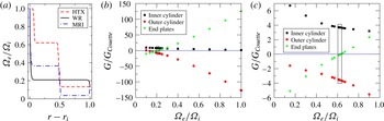
Different configurations of this apparatus differ from one another in the number of rings into which the end plates are split. Here, we study in detail two configurations, the so-called HTX and wide ring (WR), in which only one ring rotates differentially with respect to the cylinders. In the HTX configuration (dashed line in figure 1
a) the end plates are split into three rings. The inner and outer rings are attached to the cylinders, whereas the central ring rotates at an angular velocity
 $\unicode[STIX]{x1D6FA}_{e}$
intermediate to those of the cylinders. In the WR configuration (solid line in figure 1
a) there is a single ring that spans the entire annulus but also rotates independently. The dot-dashed line in figure 1(a) illustrates the boundary conditions of Ji et al. (Reference Ji, Burin, Schartman and Goodman2006), who designed their device to study the magnetorotational instability by using electrically conducting fluids and an imposed axial magnetic field. We will refer to this configuration as MRI.
(a) Rotation speed of the end plates (
 $\unicode[STIX]{x1D6FA}_{e}$
) normalized by the rotation speed of the inner cylinder (
 $\unicode[STIX]{x1D6FA}_{i}$
) in the WR, HTX and MRI configurations. (b) Torque (
 $G$
) on the cylinders and end plates in the WR configuration as a function of
 $\unicode[STIX]{x1D6FA}_{e}$
.
 $G$
is normalized by the torque of the Couette profile (1.1) (
 $G_{Couette}$
). The optimal rotation range is enclosed in a rectangular box. (c) Same as in (b) for the HTX configuration. In both (b,c) torques were computed at
 $R_{s}=644$
.

2.1 Numerical method
The Navier–Stokes equations have been solved in cylindrical coordinates using a second-order time-splitting method (Hughes & Randriamampianina Reference Hughes and Randriamampianina1998; Mercader, Batiste & Alonso Reference Mercader, Batiste and Alonso2010). The spatial discretization is via a Galerkin–Fourier expansion in
 $\unicode[STIX]{x1D703}$
and Chebyshev collocation in
 $r$
and
 $z$
. Hereafter the radial
 $u$
, azimuthal
 $v$
and axial
 $w$
velocities are normalized with respect to the characteristic velocity
 $\tilde{S}d$
used in the definition of the shear Reynolds number (2.1). The code used is a parallelized version of a spectral solver that has been widely tested (Avila et al.
Reference Avila, Grimes, Lopez and Marques2008; Lopez & Marques Reference Lopez and Marques2015; Lopez, Marques & Avila Reference Lopez, Marques and Avila2015). Details of the parallelization strategy can be found in Shi et al. (Reference Shi, Rampp, Hof and Avila2015).
In the WR and HTX configurations there are discontinuities in the angular velocity at the junctions where elements rotating at different speeds meet. For an accurate use of spectral techniques these discontinuities must be regularized (see Lopez & Shen Reference Lopez and Shen1998). In the WR configuration this is accomplished through the introduction of two exponential functions in the form
 $$\begin{eqnarray}\unicode[STIX]{x1D6FA}(r)=\unicode[STIX]{x1D6FA}_{e}+(\unicode[STIX]{x1D6FA}_{o}-\unicode[STIX]{x1D6FA}_{e})\text{e}^{-(r-r_{o})/\unicode[STIX]{x1D716}}+(\unicode[STIX]{x1D6FA}_{i}-\unicode[STIX]{x1D6FA}_{e})\text{e}^{(r-r_{i})/\unicode[STIX]{x1D716}},\end{eqnarray}$$
whereas in the HTX configuration two hyperbolic tangent functions are used
 $$\begin{eqnarray}\unicode[STIX]{x1D6FA}(r)=0.5(\unicode[STIX]{x1D6FA}_{i}+\unicode[STIX]{x1D6FA}_{o}+(\unicode[STIX]{x1D6FA}_{o}-\unicode[STIX]{x1D6FA}_{e})\,\tanh ((r-\hat{r_{o}})/\unicode[STIX]{x1D716})+(\unicode[STIX]{x1D6FA}_{e}-\unicode[STIX]{x1D6FA}_{i})\,\tanh ((r-\hat{r_{i}})/\unicode[STIX]{x1D716})),\end{eqnarray}$$
where
 $\hat{r_{o}}=r_{i}+0.48$
and
 $\hat{r_{i}}=r_{i}+0.071$
are the radial locations at which the central ring meets the outer and inner rings, respectively. In both cases
 $\unicode[STIX]{x1D716}=0.01$
was used.
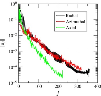
The numerical resolution was carefully chosen in order to meet several requirements. First, we checked that the total angular momentum flux through cylinders and end plates vanished in the statistically stationary regime. Second, we gradually increased the number of collocation points until converged values of the torque at the inner and outer cylinders were obtained. Finally, we checked the spectral convergence of the code using the infinity norm of the spectral coefficients of the computed solutions, defined as
 $\Vert a_{l}\Vert _{\infty }=\max _{n,m}\,|a_{l,n,m}|$
for the radial direction, and analogously for the axial and azimuthal directions. An example of spatial convergence is illustrated in figure 2, which shows
 $\Vert a_{j}\Vert _{\infty }$
, with
 $j=l,n,m$
, of the radial velocity
 $u$
for a solution corresponding to the HTX configuration at
 $R_{s}=25\,747$
. This solution was computed with
 $L=360$
and
 $N=221$
Chebyshev axial points in
 $r$
and
 $z$
, and
 $M=320$
Fourier modes in
 $\unicode[STIX]{x1D703}$
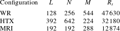
. In all simulations the trailing coefficients of the spectral expansion were at least four orders of magnitude smaller than the leading coefficients. Table 1 shows the spatial resolution corresponding to the largest
 $R_{s}$
simulated for each configuration. The reader is referred to Brauckmann & Eckhardt (Reference Brauckmann and Eckhardt2013) for a comprehensive analysis on the suitability of these convergence criteria for Taylor–Couette flows at large Reynolds numbers.
Convergence of the spectral coefficients of the radial velocity
 $u$
in the three spatial directions using the infinity norm. It corresponds to a simulation of the HTX configuration at
 $R_{s}=25\,747$
. This solution has been computed with
 $L=360$
Chebyshev radial points,
 $M=320$
Fourier modes and
 $N=221$
Chebyshev axial points.

Maximum spatial resolution and
 $R_{s}$
for each configuration.
 $L$
,
 $N$
and
 $M$
indicate the number of spectral modes in the radial, azimuthal and axial directions, respectively.

2.2 Optimal boundary conditions
Following Edlund & Ji (Reference Edlund and Ji2015), we here determine the optimal rotation speed of the end plates from a balance of the angular momentum fluxes (torque) through the boundaries of the apparatus. In particular, optimal rotation is identified when the torque at the end plates (
 $G_{e}$
) becomes zero, so that the torque on the cylinders has the same magnitude but opposite sign,
 $G_{i}=-G_{o}$
, as in the infinite-cylinder idealization. Figure 1(b,c) show the torque across the cylinders and end plates as a function of
 $\unicode[STIX]{x1D6FA}_{e}$
for solutions computed at
 $R_{s}=644$
in both configurations. In agreement with Edlund & Ji (Reference Edlund and Ji2015), in both cases there exists a narrow range of
 $\unicode[STIX]{x1D6FA}_{e}$
for which
 $G_{e}=0$
is approximately fulfilled (rectangular box in figure 1
b,c). For our simulations we chose
 $\unicode[STIX]{x1D6FA}_{e}=0.62\unicode[STIX]{x1D6FA}_{i}$
(HTX) and
 $\unicode[STIX]{x1D6FA}_{e}=0.21\unicode[STIX]{x1D6FA}_{i}$
(WR). Note that the torque in the WR configuration is substantially larger than in the HTX set-up. The reason for this will be discussed in § 3, along with the description of the secondary flows in both set-ups.
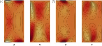
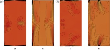
Meridional sections
 $(r,z)$
showing colour maps of the radial (left-hand panel) and axial (right-hand panel) velocities in the WR (a) and HTX (b) configurations. The solutions depicted correspond in both cases to laminar flow computed at
 $Re_{s}=644$
. In all figures shown in this paper, dark (light) regions indicate zones of positive (negative) velocities. There are
 $20$
contours equally distributed in
 $u\in [-0.08,0.06]$
,
 $w\in [-0.11,0.11]$
and
 $u\in [-0.02,0.08]$
,
 $w\in [-0.07,0.07]$
for the WR and HTX configurations, respectively.

3 Basic flow and transition to turbulence
3.1 Wide ring
Figure 3(a) shows that in the WR configuration the secondary EC cells extend over the entire annulus. Near the end plates, the flow is deflected radially towards the cylinders, leading to two Ekman vortices with opposite sense of circulation. The size and intensity of these vortices change with
 $\unicode[STIX]{x1D6FA}_{e}$
and it is only under optimal boundary conditions that these have nearly equal size and strength (
 $\max |u|=0.08$
). When the fluid reaches the cylinders it is transported from the end plates to the mid-plane over Stewartson boundary layers. As a result, two strong radial jets emerge from the cylinders and displace the flow towards mid-gap. The circulation cycle is then closed by two vertical cells that transport the fluid back to the end plates.
These large-scale secondary flows lead to linear instabilities that manifest themselves at the equatorial region (Avila et al.
Reference Avila, Grimes, Lopez and Marques2008; Avila Reference Avila2012), and cause a transition to turbulence at low values of
 $R_{s}$
. Figure 4(a) shows, through isosurfaces of the radial velocity
 $u$
, the location of the most unstable mode at the onset of instability. Note that the axisymmetric part of
 $u$
has been subtracted to facilitate visualization. The flow pattern emerging from this primary transition, which takes place at
 $R_{s}\approx 865$
, is a rotating wave with azimuthal wavenumber
 $m=2$
. As
 $R_{s}$
is further increased, the flow undergoes secondary instabilities, leading to either rotating waves with different
 $m$
or quasi-periodic states, and becomes eventually turbulent at
 $R_{s}\approx 3218$
. Figure 4(c) shows isosurfaces of
 $u$
for a turbulent state computed at
 $R_{s}=3862$
. Interestingly, the turbulence does not extend towards the end plates but remains concentrated around the mid-plane.
3.2 HTX
Figure 3(b) shows that in the HTX configuration the secondary EC is mainly confined to the vicinity of the end plates. Because of the split end plates, the radial flow along them is arranged in four alternating outward–inward vortices which direct the flow towards the junctions between the rings. The pair of vortices located at the outermost part of the end plates are significantly larger and more intense (
 $\max |u|=0.08$
) than those arising near the inner cylinder (
 $\max |u|=0.02$
). Significant axial transport of fluid towards the mid-plane occurs only in a narrow region around mid-gap. However, the flow does not reach the mid-plane, as it is recirculated towards the inner cylinder by a strong radial inflow that arises at an approximately intermediate distance between the end plates and the equatorial region. Finally, the flow is pushed back towards the end plates by axial velocities arising in the regions near the cylinders. A comparison with the WR configuration reveals that the substantial difference in torque shown in § 2.2 is caused by the influence of the Stewartson boundary layers that form at the cylinders in the WR configuration. These produce strong azimuthal velocity gradients near the cylinders, which result in a significant increase of the torque as compared with that in the HTX configuration.
The meridional circulation in the HTX configuration becomes unstable at
 $R_{s}\approx 727$
. The instability results in a rotating wave with
 $m=5$
localized at the end plates (see figure 4
b), and the flow becomes quickly chaotic as
 $R_{s}$
is increased (
 $R_{s}\approx 1287$
). Nevertheless, the turbulence remains primarily localized near the upper and lower third of the experiment (see figure 4
d), so that the zonal flow at the equatorial region is barely affected by the secondary flows and nearly matches a quasi-Keplerian velocity profile, see § 4.2.
(a,b) show isosurfaces of the radial velocity of the leading eigenmodes near the onset of instability. The axisymmetric component has been subtracted to facilitate visualization of the spatial structure of the unstable mode. (a) Equatorial rotating wave with
 $m=2$
computed at
 $R_{s}=772$
in the WR configuration. (b) Rotating wave with
 $m=5$
localized near the end plates for
 $R_{s}=901$
in the HTX configuration. (c,d) show isosurfaces of the radial velocity for turbulent states computed at
 $R_{s}=3862$
in the WR (c) and HTX (d) configurations. There are six isosurfaces equally distributed across
 $u\in [-0.13,0.12]$
and
 $u\in [-0.09,0.14]$
in the WR and HTX configurations, respectively.

4 Dynamics at high Reynolds numbers
As the rotation of the cylinders is increased the spatial arrangement of the secondary flows undergoes significant changes in both configurations, which alter the structure of the resulting turbulence. While this transition occurs smoothly with increasing
 $R_{s}$
, we here distinguish between low and high Reynolds numbers using
 $R_{s}\approx 10^{4}$
as an approximate threshold, beyond which the changes described in this section begin to become apparent.
Meridional sections
 $(r,z)$
showing colour maps of the mean radial (left-hand panel) and axial (right-hand panel) velocities in the WR (a) and HTX (b) configurations. The solutions depicted were computed at
 $R_{s}=19\,310$
in (a) and
 $R_{s}=22\,529$
in (b). There are
 $20$
contours equally distributed in
 $u\in [-0.16,0.08]$
,
 $w\in [-0.17,0.17]$
and
 $u\in [-0.07,0.10]$
,
 $w\in [-0.06,0.06]$
for the WR and HTX configurations, respectively.

4.1 Wide ring
Figure 5(a) shows the structure of the time-averaged secondary flow for the WR configuration at
 $R_{s}=19\,302$
. Here the radial jets that emanate from the cylinders at the equatorial region do not extend across the entire gap, but remain localized in regions closer to the cylinders. The gradual displacement of these jets towards the cylinders as
 $R_{s}$
increases is accompanied by the emergence of two pairs of radial flow cells on top and bottom of them. These radial cells recirculate the flow towards the cylinders, so that the vertical transport of fluid from the equator towards the end plates that closes the Ekman circulation cycle is also confined to the vicinity of the cylinders. As a result, the radial and axial velocities are nearly zero over the central region of the gap, and the flow becomes essentially azimuthal in the bulk, resulting in vanishing Reynolds stresses.
The turbulent dynamics of this system is confined to the region in which the radial equatorial jets penetrate into the bulk flow. Hence as
 $R_{s}$
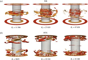
increases and the secondary flows occupy regions closer to the cylinders, significant turbulent fluctuations are only found in the vicinity of the cylinders. Figure 6(a) clearly illustrates the progressive localization of the turbulence near the cylinders as
 $R_{s}$
increases. Interestingly, turbulent structures occur mainly near the inner cylinder, which could be related to the large curvature of the apparatus (
 $\unicode[STIX]{x1D702}=r_{i}/r_{o}=0.3478$
).
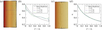
Figure 7(a) shows the mean azimuthal velocity
 $v$
for
 $R_{s}=47\,630$
. With the exception of the zones near the cylinders, where the flow is obviously affected by the turbulence, it is observed that
 $v$
is nearly independent of the axial coordinate. This is confirmed in figure 7(b), where
 $v(r)$
is shown at three different axial locations. Although these profiles collapse together, they differ substantially from the desired quasi-Keplerian velocity profile (1.1), shown as a (black) solid line in figure 7(b). Interestingly, despite vanishing fluctuations (and hence Reynolds stresses) in the bulk, the profile is far from ideal because of the effect of the global EC.
Evolution of the isosurfaces of the radial velocity
 $u$
with
 $R_{s}$
in both configurations. There are two isosurfaces corresponding to
 $u=\pm 0.04$
in both cases. Note that plots corresponding to the WR configuration are slightly tilted to better illustrate the gradual displacement of the turbulence towards the cylinders.

(a,c) show colour maps and contours illustrating the mean azimuthal velocity
 $v$
in the WR and HTX configurations, respectively, whereas radial profiles of
 $v$
computed at three different axial locations are shown in (b) WR and (d) HTX. In both cases the solution depicted corresponds to the maximum
 $R_{s}$
achieved in our simulations,
 $R_{s}=47\,630$
in (a,b), and
 $R_{s}=32\,180$
in (c,d). There are
 $40$
contours equally distributed across the full range of
 $v$
. The solid (black) line shows the quasi-Keplerian velocity profile (1.1) that would be achieved. The horizontal lines superimposed upon (a) indicate the axial locations at which the azimuthal velocity profiles have been computed.

4.2 HTX
Figure 5(b) shows the structure of the time-averaged secondary meridional flow for the HTX configuration at
 $R_{s}=22\,529$
. As
 $R_{s}$
increases both radial and axial velocities are progressively confined to the end plates, resulting in an increasingly larger region where the flow remains nearly purely azimuthal. There is a fraction of the secondary flow generated at the end plates that is transported to the equator over a boundary layer at the inner cylinder. The formation of this boundary layer leads to the emergence of two large-scale circulation cells, which are progressively confined to the inner cylinder as
 $R_{s}$
is increased. These cells are similar to but significantly weaker than those in the WR configuration. Turbulent fluctuations are also progressively confined to the end plates as
 $R_{s}$
increases (see figure 6
b). Some fluctuations caused by the large-scale recirculation flow may also occur in the vicinity of the inner cylinder. However, given their low intensity, it can be stated that the flow remains nearly laminar when sufficiently far from the end plates.
As seen in figure 7(c), the mean azimuthal velocity is only significantly affected by the secondary flows in the vicinity of the end plates. Hence, negligible differences were found when measuring radial profiles of the mean azimuthal velocity in the bulk at different axial locations (see figure 7
c). Despite large-scale secondary flows developing at the inner cylinder, unlike for the WR configuration, these are not sufficiently strong as to significantly modify the azimuthal velocity. As a result, the azimuthal velocity profiles in this configuration closely approximate the desired quasi-Keplerian Couette flow (1.1). It should be noted that Edlund & Ji (Reference Edlund and Ji2014) reported velocity profiles with small but noticeable deviations from (1.1) near the inner cylinder. Such deviations suggest that, while the turbulence at the inner cylinder does not affect the bulk flow in our simulations, its influence might not be entirely negligible in experiments at larger
 $R_{s}$
.
4.3 Dynamics of the MRI configuration
Avila (Reference Avila2012) performed direct numerical simulations of the MRI configuration of Ji et al. (Reference Ji, Burin, Schartman and Goodman2006) up to
 $R_{s}=6437$
, for which turbulence was found to fill the entire domain. Here we extend the range of Reynolds numbers by a factor of two. First of all, we note that the rotation speeds of the end-plate rings used by Ji et al. (Reference Ji, Burin, Schartman and Goodman2006) are not optimal, and result in large torque at the end plates. At low
 $R_{s}$
, the meridional circulation resembles that of the WR configuration (see figure 1 in Avila Reference Avila2012), with a strong radial jet located at the equatorial region. However, unlike the WR, the radial flow at the end plates is entirely inward, and so there is a single large-scale circulation cell in the upper and lower half of the experiment. As in the WR configuration the large-scale circulation cells and turbulent motions cluster here progressively near the inner cylinder (see figure 8
a,b), leaving a nearly azimuthal and laminar flow in the remaining part of the gap.
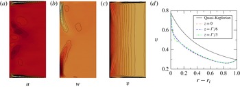
Figure 8(c,d) shows the time-averaged azimuthal velocity
 $v$
and radial profiles of
 $v$
at
 $R_{s}=12\,874$
, respectively. Here
 $v(r)$
is also nearly uniform in the axial direction, but differs from the theoretical Couette flow (1.1). Hence we conclude that although Ji et al. (Reference Ji, Burin, Schartman and Goodman2006) measured negligible Reynolds stresses in the bulk of their experiment, their flows were strongly turbulent in thin boundary layers at the cylinders. Interestingly, in the bulk the profiles are in fact quasi-Keplerian, yet substantially shifted with respect to Couette flow because of the sharp drop at the cylinder boundary layers. Similar velocity profiles for this configuration were reported in the numerical simulations of Obabko, Cattaneo & Fischer (Reference Obabko, Cattaneo and Fischer2008) and experiments of Schartman et al. (Reference Schartman, Ji, Burin and Goodman2012), who speculated that the deviation in the profiles near the inner cylinder might be caused by the existence of turbulent Stewartson boundary layers.
(a–c) show meridional sections
 $(r,z)$
illustrating the mean radial, axial and azimuthal velocities in the MRI configuration for a solution computed at
 $R_{s}=12\,874$
.
 $20$
contours equally distributed across
 $u\in [-0.15,0.03]$
,
 $w\in [-0.17,0.17]$
and
 $v\in [0.06,0.78]$
have been added. (d) Radial profiles of
 $v$
computed at the same axial locations as in figure 7.

5 Discussion and conclusions
We have performed direct numerical simulations of the flow in a Taylor–Couette device that Edlund & Ji (Reference Edlund and Ji2014) specifically designed to infer the hydrodynamic stability of constant-density Keplerian flows. A first interesting observation is that the occurrence of turbulence at low
 $R_{s}$
appears to be a robust feature of quasi-Keplerian Taylor–Couette flows. Nevertheless, turbulence manifests itself differently depending on axial boundary conditions. In the WR configuration, as well as in the HTX and MRI configurations if the boundary conditions are not optimal, as in Ji et al. (Reference Ji, Burin, Schartman and Goodman2006), the end plates drive a large-scale EC which gives rise to strongly turbulent boundary layers at the cylinders. In contrast, when the HTX configuration is operated under optimal boundary conditions, the EC and associated turbulence are localized near the end plates.
As
 $R_{s}$
increases, turbulence localizes to thin boundary layers, whereas the flow in the bulk becomes nearly azimuthal and axially uniform. The progressive relaminarization of the bulk flow observed in these configurations does not however imply that they are all adequate to infer the stability of astrophysical flows. As reported in Edlund & Ji (Reference Edlund and Ji2015), the azimuthal velocity profiles achieved in the WR configuration differ substantially from a quasi-Keplerian profile, even in their optimal regime of operation, whereas laminar Couette profiles can be realized in the HTX configuration with optimal boundary conditions. Leclercq et al. (Reference Leclercq, Partridge, Augier, Dalziel and Kerswell2016) showed that quasi-Keplerian profiles can also be achieved in experiments if stable stratification is added near the end plates. However, this method becomes impractical for the large Reynolds numbers investigated in the Princeton experiments.
It is remarkable that in spite of the nearly one order of magnitude gap in Reynolds numbers between our simulations and the experiments of Edlund & Ji (Reference Edlund and Ji2015), the azimuthal velocity profiles are indistinguishable. This suggests that, despite the turbulent boundary layers, the velocity profiles exhibit self-similar behaviour, in agreement with the observations (Edlund & Ji Reference Edlund and Ji2015). Taken together, these results show that isothermal constant-density quasi-Keplerian Taylor–Couette flows are stable at least up to
 $R_{s}=O(10^{6})$
. Noteworthy, for
 $\unicode[STIX]{x1D702}=0.3478$
and
 $Re=10^{6}$
the energy of disturbances imposed to the laminar flow can be transiently amplified up to a factor of
 $G=408$
(see (5.1) in Maretzke, Hof & Avila Reference Maretzke, Hof and Avila2014). Hence it seems that for quasi-Keplerian flows linear transient growth is a poor indicator of turbulence transition.
Our results highlight that experiments on astrophysical flows cannot rely on measuring velocity fluctuations alone, because vanishing Reynolds stresses do not imply quasi-Keplerian velocity profiles. Similarly, torque measurements are inadequate because they cannot be used to infer the level of turbulence in the bulk, which may be laminar despite highly turbulent boundary layers.
We remark that the experiments simulated here were performed with a constant-density fluid, whereas in accretion disks the gas is strongly stratified in the axial and radial directions. Hence the results shown here apply to barotropic gases only. For stratified quasi-Keplerian flows several instabilities have been reported. Examples are the strato-rotational instability (Molemaker, McWilliams & Yavneh Reference Molemaker, McWilliams and Yavneh2001; Le Bars & Le Gal Reference Le Bars and Le Gal2007), the radiative instability (Le Dizès & Riedinger Reference Le Dizès and Riedinger2010; Riedinger, Le Dizès & Meunier Reference Riedinger, Le Dizès and Meunier2011), the zombie vortex instability (Marcus et al. Reference Marcus, Pei, Jiang, Barranco, Hassanzadeh and Lecoanet2015; Lesur & Latter Reference Lesur and Latter2016), the vertical shear instability (Urpin & Brandenburg Reference Urpin and Brandenburg1998; Nelson, Gressel & Umurhan Reference Nelson, Gressel and Umurhan2013) and the subcritical global instability (Klahr & Bodenheimer Reference Klahr and Bodenheimer2003; Johnson & Gammie Reference Johnson and Gammie2006; Petersen et al. Reference Petersen, Julien and Stewart2007). The ability to realize quasi-Keplerian velocity profiles in experiments at large Reynolds numbers opens up avenues for new experimental investigations of some of these instabilities and their underlying mechanisms. Candidates are the vertical shear instability or subcritical global instability, which could be addressed with experiments on radially stratified Taylor–Couette flows including thermal relaxation, or the zombie vortex instability, which could be studied in a Taylor–Couette set-up subject to strong stable stratification in the vertical direction. Nevertheless, additional issues related to the interplay between end plates and stratification must first be addressed (Lopez et al. Reference Lopez, Marques and Avila2015).
Acknowledgements
This work was partially supported by the Spanish Government grant FIS2013-40880-P and BES-2010-04154. We are grateful to red Española de Supercomputación (RES) and the Regionales Rechenzentrum Erlangen (RRZE) for the computational resources provided.