What is being timed?

A TTE estimate first identifies the entity being timed, which might be a local population, a metapopulation a species or a clade, represented in a model by state variables such as abundance, occupancy or reproductive output. Loss of reproductive viability, functional extinction, ecological extinction, quasi-extinction and species extinction are related endpoints, but they do not answer the same question. A local population can be lost while the species persists elsewhere; a species can be functionally absent from an ecosystem before the last individual dies; a model can cross a quasi-extinction threshold while recovery remains possible.

The same interpretive choice applies to the start point, which in conservation settings might be model initialisation, first detection of decline, formal listing, onset of a threat or the implementation of a management decision. In historical accounts, the clock often begins with habitat transformation, overharvest, disease introduction or predator arrival, while the last robust evidence of persistence usually constrains the endpoint. In palaeobiology, it is typically constrained by stratigraphic intervals, fossil horizons, radiometric dates or inferred environmental change.

Nor is the endpoint a trivial stopping rule, even when the word “extinction” seems unambiguous. Strict biological extinction is the death of the last individual, but this event is almost never observed (Solow, Reference Solow1993). Conservation modelling can measure extinction at zero abundance, quasi-extinction below a decision threshold or loss of demographic viability (Brook et al., Reference Brook, O’Grady, Chapman, Burgman, Akçakaya and Frankham2000), whereas palaeontological analyses often estimate the unobserved end of a taxon’s true temporal range from sampled occurrences (Signor and Lipps, Reference Signor, Lipps, Silver and Schultz1982). The same word can therefore describe a forecast, an inferred extinction window, a waiting-time distribution or a realised taxon duration. A clear estimate states the entity, start point, endpoint, evidence stream and uncertainty structure before interpreting the interval.

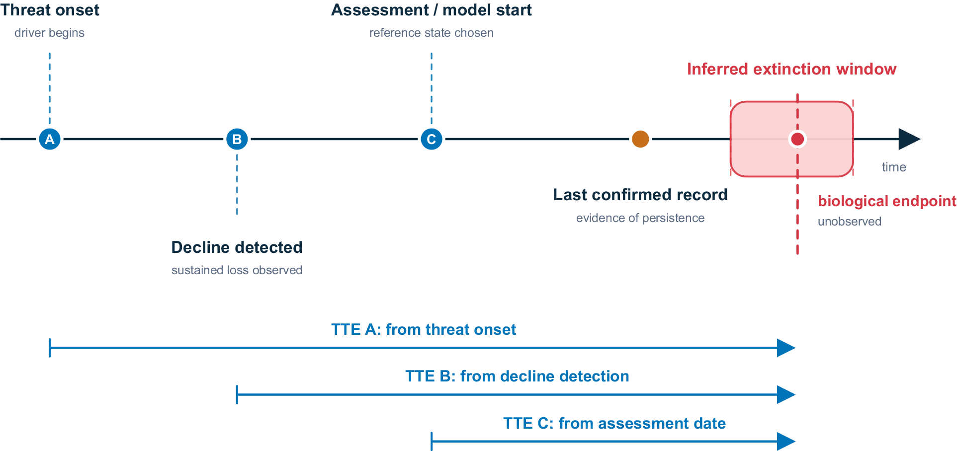
Because entity, start point and endpoint all do substantive work, neighbouring terms need to be kept distinct. Extinction risk, extinction debt, extinction lag, quasi-extinction, last appearance datum, inferred extinction, functional extinction and ecological extinction can all modify the clock, but each carries its own endpoint and evidence standard. TTE becomes comparable across cases only when those boundary conditions are made visible (Figure 1).

Figure 1.

One extinction, several clocks. Time to extinction is an elapsed interval only after the clock has been named. The same endpoint definition can yield different estimates depending on whether timing begins at the onset of a threat (TTE A), the first detection of sustained decline (TTE B), formal assessment or predictive-model initialisation (TTE C) or another explicit start point. The last confirmed record is evidence of persistence to that point in time. The true biological endpoint is often unobserved and is therefore better represented as an inferred extinction window (red box) than as a single known date. The relative positions of events are schematic rather than to scale; uncertainty is represented along the time axis.

Figure 1. Long description

A horizontal black arrow pointing right represents the progression of time. Along this axis, several key events are marked.

* Point A is labeled Threat onset driver begins. It is marked with a blue circle.

* Point B is labeled Decline detected sustained loss observed. It is marked with a blue circle.

* Point C is labeled Assessment forward slash model start reference state chosen. It is marked with a blue circle.

* A solid orange circle follows, labeled Last confirmed record evidence of persistence.

* A red shaded rectangle labeled Inferred extinction window surrounds a central red dot on a dashed vertical line. This point is labeled biological endpoint unobserved.

Below the main timeline, three blue horizontal arrows indicate the duration of different T T E measurements, all terminating at the biological endpoint.

* T T E A from threat onset begins at the vertical alignment of Point A.

* T T E B from decline detection begins at the vertical alignment of Point B.

* T T E C from assessment date begins at the vertical alignment of Point C.

Forward estimates in conservation biology

In prospective conservation work, TTE asks how long a population is expected to persist before crossing an extinction or quasi-extinction endpoint under specified demographic, threat, environmental and management assumptions. PVA is a standard applied framework for this problem (Boyce, Reference Boyce1992).

In stochastic projection, each replicate either first crosses an extinction or quasi-extinction endpoint at a particular time or remains uncrossed by the chosen time horizon. The probability of extinction (PE) or quasi-extinction (PQE) is the fraction of replicates crossed over that horizon, with a zero threshold for PE and a threshold above zero for PQE. TTE summaries describe when crossing occurs and how those crossing times are distributed. Minimum viable population analysis uses the related perspective of asking what population size is needed to keep PE acceptably low over a chosen time horizon (Shaffer, Reference Shaffer1981).

The distinction is important because, unlike TTE, PE and PQE are bounded cumulative summaries. If all replicates go extinct by a given horizon (PE = 1), these metrics cannot distinguish immediate collapse from slower failure. In one case, all replicates might be lost early because initial abundance is low; in another, replicates might decline chronically to extinction from high initial abundance. PE = 1 for both, but the timing and distribution of extinction are very different. Means, medians, quantiles, survival curves and the shape of the extinction-time distribution therefore add diagnostic information for comparing management scenarios, sensitivities and novel risks.

Because the output is conditional, the time scale cannot be separated from the assumptions. A forecast over 20 years and a forecast over 100 years might imply different management priorities even for the same population. Over finite horizons, some trajectories might not cross the endpoint, so mean TTE can be conditional (e.g., only relevant to extinct populations or replicates), right-censored, extrapolated or undefined. Likewise, a threshold chosen for regulatory action may be appropriate for triage while remaining different from biological extinction.

Extinction-time distributions also reflect model mechanisms, because demographic, genetic and environmental stochasticity, random catastrophes, density dependence, mating system, Allee effects, spatial structure and management interventions all alter the clock (Lande, Reference Lande1993; Sæther et al., Reference Sæther, Engen, Lande, Møller, Bensch, Hasselquist, Beier and Leisler2004; Melbourne and Hastings, Reference Melbourne and Hastings2008). Two populations with the same abundance can therefore have different expected persistence times if their variance structure, spatial structure or demographic architecture differs.

This makes TTE useful for decision support, especially when fixed-horizon PE (or PQE) is equal across alternatives or when comparisons among management scenarios are relative rather than absolute. A recent PVA for the Eastern Iberian Reed Bunting (Emberiza schoeniclus witherbyi), for example, evaluated extinction probabilities over multiple horizons and estimated mean extinction times under baseline and management scenarios, showing how intervention could delay or avert projected extinction (Alambiaga et al., Reference Alambiaga, Vera and Monrós2025). Such studies are most informative when they make assumptions, endpoints and uncertainty visible. PVA reporting protocols and modern appraisals stress that forecasts should be tied to model structure, input data, scenario realism and uncertainty (Pe’er et al., Reference Pe’er, Matsinos, Johst, Franz, Turlure, Radchuk, Malinowska, Curtis, Naujokaitis-Lewis, Wintle and Henle2013; Chaudhary and Oli, Reference Chaudhary and Oli2020).

Backward estimates in historical and palaeontological records

Historical and palaeontological studies often face the reverse problem: an extinction event has probably occurred, or almost certainly occurred in deep-time cases, but the timing is uncertain. The evidence is a sequence of sightings, specimens, dated remains, fossils, environmental DNA, search records or non-detections. The task is to infer an endpoint from an incomplete observation process.

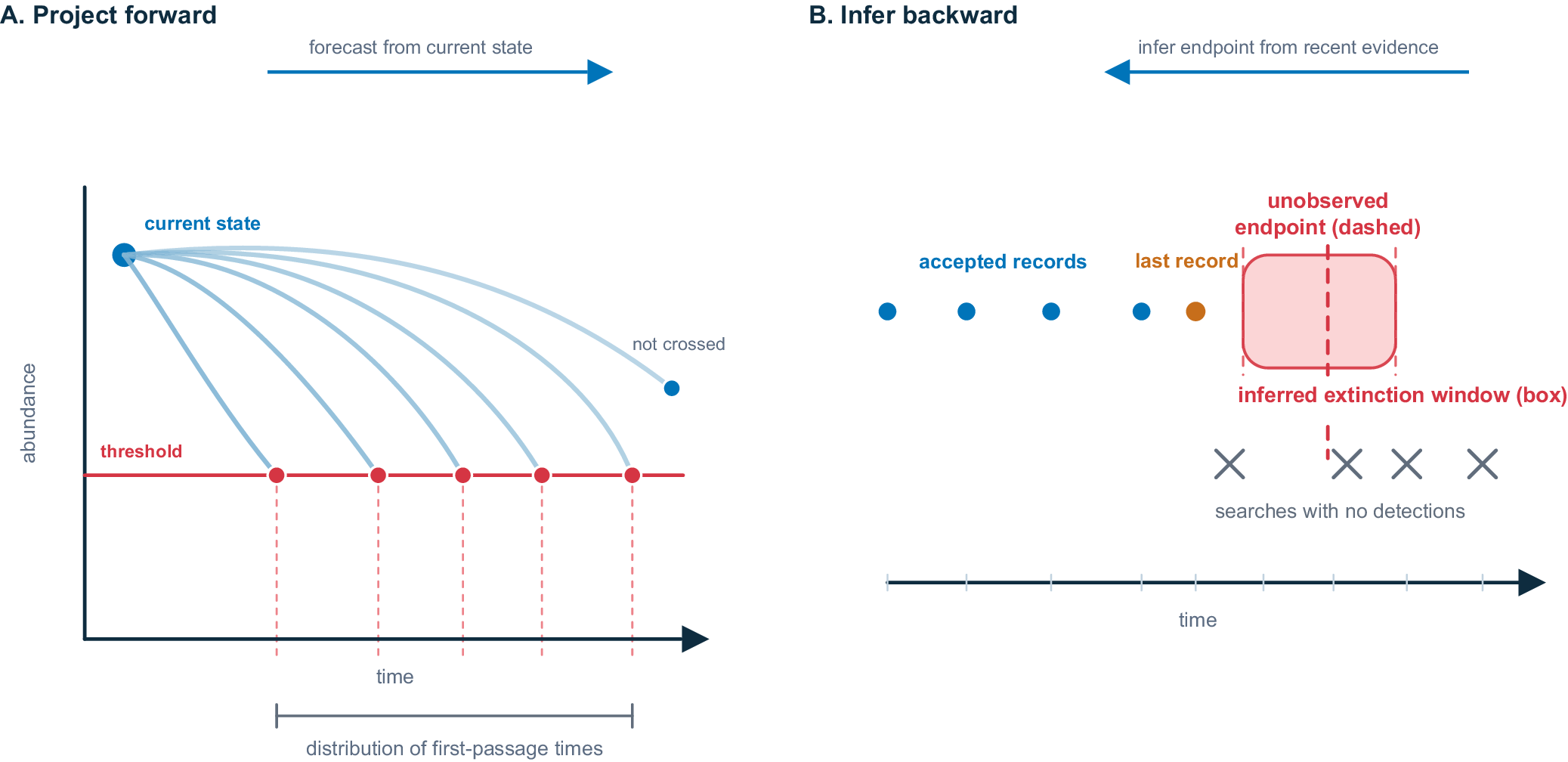
Retrospective studies typically estimate the endpoint first; the elapsed TTE then depends on the chosen starting point, such as first appearance, onset of decline, arrival of a threat or the beginning of the sampled interval (Figure 1). A last record confirms persistence at a particular time, but by itself does not locate the extinction event (Figure 2). Sighting-record methods treat this as an endpoint-estimation problem (Solow, Reference Solow1993). The Dodo (Raphus cucullatus) provides a useful illustrative example here because statistical treatment of sighting records placed the inferred extinction time later than the last accepted observation (Roberts and Solow, Reference Roberts and Solow2003). For recently extinct or possibly extant mammals, rediscovery patterns and detectability show why absence of recent records must be interpreted through search effort, range, conspicuousness and taxonomy (Fisher and Blomberg, Reference Fisher and Blomberg2011). In this setting, TTE includes uncertainty in both the biological process and the observation process.

Figure 2.

Two inferential directions for time to extinction. In prospective conservation analyses, time to extinction is commonly estimated by projecting population trajectories forward from an observed or modelled current state until they first cross an extinction or quasi-extinction threshold; the result is a distribution of first-passage times, rather than a deterministic countdown. In historical and palaeontological analyses, the direction of inference is reversed: accepted records, dated remains, fossils, environmental DNA, search effort and non-detections are used to infer an unobserved extinction window after the last confirmed evidence of persistence. In both cases, the estimate depends on the endpoint, evidence stream, observation process and uncertainty model.

Figure 2. Long description

Panel A, titled Project forward, shows a graph with abundance on the y-axis and time on the x-axis. A blue dot at the top-left represents the current state. Multiple light blue curved lines descend from this point. Most lines intersect a horizontal red line labeled threshold. Red dots mark these intersections, with vertical dashed lines dropping to the x-axis to form a distribution of first-passage times. One line remains above the threshold, labeled not crossed. A blue arrow above the graph points right, labeled forecast from current state.

Panel B, titled Infer backward, features a horizontal time axis. From left to right, a series of blue dots represents accepted records, followed by an orange dot labeled last record. To the right of the last record is a pink shaded rectangle labeled inferred extinction window box. Inside this box, a vertical red dashed line indicates the unobserved endpoint dashed. Below the timeline, a series of X marks represents searches with no detections. A blue arrow above the panel points left, labeled infer endpoint from recent evidence.

The same endpoint problem reappears over longer timescales in palaeontology, where fossil occurrences are samples from an incomplete temporal record and the youngest known fossil of a taxon usually predates its true extinction. This is the Signor–Lipps effect in general form: incomplete sampling makes observed last appearances biased proxies for true extinction times (Signor and Lipps, Reference Signor, Lipps, Silver and Schultz1982). Statistical methods for range endpoints estimate confidence or probability intervals around true first and last appearances, rather than assuming that observed appearances are exact boundaries (Strauss and Sadler, Reference Strauss and Sadler1989; Marshall, Reference Marshall2010). At broader palaeobiological scales, inferred first and last appearances are also assembled into taxon durations, survivorship curves and extinction hazards, but these summaries inherit the same sampling and taxonomic uncertainties (Alroy, Reference Alroy2008). The same logic applies when radiocarbon dates, archaeological occurrences or ancient environmental DNA signals extend or complicate inferred extinction windows. Debates over mammoth persistence show how new evidence streams can shift the apparent endpoint while also introducing their own preservation and contamination uncertainties (Wang et al., Reference Wang, Pedersen, Alsos, De Sanctis, Racimo, Prohaska, Coissac, Owens, Merkel, Fernandez-Guerra, Rouillard, Lammers, Alberti, Denoeud, Money, Ruter, McColl, Larsen, Cherezova, Edwards, Fedorov, Haile, Orlando, Vinner, Korneliussen, Beilman, Bjørk, Cao, Dockter, Esdale, Gusarova, Kjeldsen, Mangerud, Rasic, Skadhauge, Svendsen, Tikhonov, Wincker, Xing, Zhang, Froese, Rahbek, Bravo, Holden, Edwards, Durbin, Meltzer, Kjær, Möller and Willerslev2021; Miller and Simpson, Reference Miller and Simpson2022).

Direct sightings, dated bones, fossils, sedimentary DNA and structured non-detections differ in temporal resolution, geographic coverage and susceptibility to error. A robust extinction-time estimate therefore needs a model of how evidence is generated and preserved, as well as a model of population persistence.

The prospective and retrospective uses of TTE are linked by a common inferential structure (Figure 2). Conservation biology projects from an observed present towards a future endpoint. Historical extinction studies and palaeontology infer from observed remnants towards an unobserved past endpoint. Both require a distinction between biological extinction and the evidence by which extinction is forecast, inferred or declared.

Why the concept matters

By linking process to consequence, TTE gives biological meaning to rapid collapse and delayed loss. Short expected times can indicate rapid threat escalation, catastrophic mortality, strong demographic vulnerability, Allee effects or late detection. Long times can indicate extinction debt, demographic lag, chronic attrition, refuge persistence or slow failure of recruitment. These interpretations are most useful when estimates are comparable in scale, endpoint and evidence basis.

That interpretive value becomes practical when managers need to compare intervention windows, decide whether monitoring is likely to detect decline before irreversible loss, and communicate urgency without reducing extinction to a countdown. A mean TTE can be useful, but the mean alone can hide a wide, skewed, bimodal or right-censored distribution of possible outcomes (Ludwig, Reference Ludwig1996). Likewise, a last sighting can be a strong datum without being a biological endpoint. Uncertainty is therefore part of what the estimate communicates.

The main misuse is to compare different clocks as if they were the same estimate. A modelled time to quasi-extinction is not directly comparable with an inferred extinction time from historical sightings or a fossil last appearance unless the endpoint, evidence basis and observation process are explicit. TTE is therefore best viewed as an operational estimate of persistence or endpoint timing.

Whether used prospectively in PVA and conservation-scenario analysis or retrospectively in historical and palaeontological inference, the scientific content of TTE lies in the named clock and its uncertainty. Useful statements specify the entity, scale, start point, endpoint, evidence stream, observation process, model assumptions and uncertainty; that discipline is what allows estimates across fields to inform one another.