


1. Introduction
In game theory, the centerpiece of analysis is the notion of equilibrium. In a game in strategic form, an equilibrium is a strategy profile at which certain types of coalitions of agents (or players) do not have profitable deviations. The strongest notion that can be defined along this line is a super strong equilibrium: no coalition of agents benefits (in the Pareto sense) from jointly changing their strategies.
Note that in a game with n agents, there are as many as
 $2^{n}-1$
(non-empty) possible coalitions if any coalition is deemed viable. However, deeming every coalition viable and disqualifying strategy profiles as non-equilibrium may be misguided. First of all, in game theory, the super strong equilibrium is a rarity. Therefore, from a pure theory perspective, imposing restrictions on coalition formation may help obtain existence results.
Footnote 1
The best-known case is the notion of a Nash equilibrium, in which coalition formation is restricted to singletons. Nash (Reference Nash1951) showed that every finite game admits a Nash equilibrium if mixed strategies are allowed. There are also results in the literature showing the existence of a pure-strategy Nash equilibrium in different game forms (see, for instance, Baye et al. Reference Baye, Tian and Zhou1993; Reny Reference Reny1999; Rosenthal Reference Rosenthal1971).
In certain settings, there may also be practical reasons to believe that not every coalition is viable. For instance, coalition formation may be restricted by institutional or self-imposed constraints. In global affairs, it is not uncommon that a government feels compelled to act in unison with its allies, even if doing so comes at a great cost. For instance, it may be forced to uphold trade sanctions on a neighboring country, causing much harm to its economy. Or, a nation may refuse to engage in mutually beneficial relations with another nation due to historical enmities. In a biological setting, an animal may not engage in behavior that would help its fitness but at the expense of the fitness of its offsprings. Of course, it is always possible to model this type of scenarios without restrictions on coalition formation if the payoff functions are defined appropriately. The costs of going against allies, the displeasure from engaging with a historical rival, or the value assigned to the fitness of offsprings can be ingrained into the payoff functions. Nevertheless, it may often be easier to work with extraneously given restrictions on coalition formation rather than with complex payoff functions. Then, one may simply assume that a government cannot coordinate with its neighbor without the consent of its allies; two nations with historical enmities do not engage with one another; and an animal never engages in behavior detrimental to the fitness of its offsprings.
There is also the information argument in support of imposing restrictions on coalition formation. A deviation by a coalition requires that coalition members act in unison. Taking coordinated action is difficult; however, if coalition members are not familiar with one another. Or, everyone may be familiar with one another, and yet taking coordinated action may be too elusive a goal when there are too many agents involved.
The subject matter of our paper is restrictions on coalition formation. As mentioned briefly above, in a game, coalition formation may be restricted by various factors, such as size, information, or institutional constraints. A full consideration of what restrictions on coalition formation may be reasonable in different real-life scenarios is beyond our scope. In this paper, we focus on restrictions that are motivated by real-life social structures. Under our restrictions, the sets of viable coalitions have simple mathematical structures, and their cardinalities are O(n) or
 $O(n^{2})$
(n is the number of agents). On the basis of our restrictions, we define new equilibrium notions, and then we study how they relate to one another.
Adding social structures to games and then studying equilibria is a growing trend in recent literature. A driving force may be the ever-growing importance in our lives of social networking websites. The following equilibrium notion, introduced in an earlier study, is related to our study in particular Footnote 2 :
-
– Partition Equilibrium: In a partition equilibrium, the set of viable coalitions is a partition of the set of agents; see Figure 1A. This notion generalizes the notion of a Nash equilibrium, and it was introduced by Feldman and Tennenholtz (Reference Feldman and Tennenholtz2010).
Examples of partition and laminar coalition structures.

Along similar lines, we introduce in our paper three new notions of equilibrium, motivated by real-life social structures:
-
– Laminar Equilibrium: In a laminar equilibrium, the set of viable coalitions exhibits a laminar structure; see Figure 1B. The laminar equilibrium generalizes the notion of a partition equilibrium. Notice that this notion relates to hierarchical communities in real life. For instance, a military is divided into corps, legions, and brigades; a cabinet is divided into ministries, departments, and directorates; a university is divided into faculties and departments; and a company is divided into business units, divisions, and departments.
-
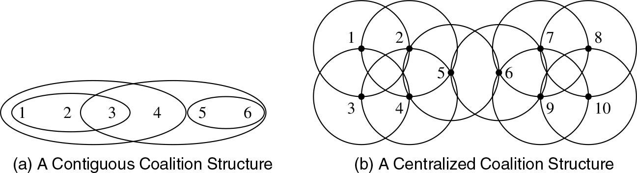
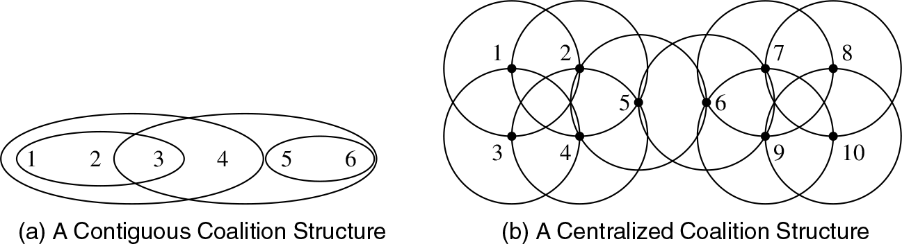
– Contiguous Equilibrium: In a contiguous equilibrium, it is assumed that agents are distributed on a line, and each viable coalition consists of some agents that are ordered on the line subsequently; see Figure 2A. Two examples that may give rise to coalition formation of this type are residents on a street who socialize via neighborhood, and electors on the left-right political spectrum who cooperate if their political views are close enough.
-
– Centralized Equilibrium: In a centralized equilibrium, it is assumed that agents are distributed on a plane, and each viable coalition corresponds to a circle on the plane: the agents that lie inside the circle are the coalition members, and one coalition member lies at the center of the circle; see Figure 2B. The agent at the circle’s center can be viewed as the coalition leader, who may call into action the agents in her neighborhood (other coalition members).
Examples of contiguous and centralized coalition structures.
Notice that, in the case of a partition equilibrium or a laminar equilibrium, the number of viable coalitions is O(n), and in the case of a contiguous equilibrium or a centralized equilibrium, the number of viable coalitions is
 $O(n^{2})$
.
Our first main result establishes a hierarchy between the above notions of equilibrium: In Theorem 1, we show that a set of viable coalitions is laminar if it is a partition, it is contiguous if it is laminar, and it is centralized if it is contiguous. Thus, our Theorem 1 shows that each equilibrium notion defined above generalizes the preceding ones. This means that in a specific game form, showing that a centralized equilibrium always exists implies that a contiguous equilibrium also always exists, and so on. Footnote 3
As an application venue for our equilibrium notions, we consider resource selection games (RSGs). Our choice of this class of games for our existence analysis is for several reasons: RSGs fall into the class of potential games, for which the existence of a Nash equilibrium is guaranteed (see Monderer and Shapley Reference Monderer and Shapley1996; Rosenthal Reference Rosenthal1971). As it turns out, however, an equilibrium may not exist if any coalition is deemed viable. Footnote 4 This renders RSGs a suitable ground for studying the existence of the above notions of equilibrium: They are more general than a Nash Equilibrium, and yet not as demanding as a super strong equilibrium. Also, RSGs are an important class of games, useful in modeling real-life scenarios in a wide range of areas, including economics, transportation, communication networks, and biology. Finally, the partition equilibrium notion has already been studied in two prior studies in the context of RSGs (see Anshelevich et al. Reference Anshelevich, Caskurlu and Hate2013; Feldman and Tennenholtz Reference Feldman and Tennenholtz2010), and therefore, by studying this class of games, we want to relate our findings to these earlier studies.
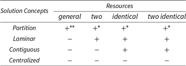
Our results in RSGs and their relation to the results in the literature are as follows: Feldman and Tennenholtz (Reference Feldman and Tennenholtz2010) showed that a partition equilibrium always exists in RSGs under the following restrictions: (i) if the size of a viable coalition is bounded by 2; or (ii) if there are only two resources; or (iii) if the resources are identical. Anshelevich et al. (Reference Anshelevich, Caskurlu and Hate2013) generalized this result by proving that a strategy profile that is both a partition equilibrium and a Nash equilibrium is guaranteed to exist in general RSGs. Footnote 5
Our findings are as follows:
-
– In Sections 3.2 and 3.4, we generalize the results in Feldman and Tennenholtz (Reference Feldman and Tennenholtz2010) ((ii) and (iii) above) to the notion of a laminar equilibrium. We prove that a laminar equilibrium always exists: (i) if there are only two resources (Theorem 5) Footnote 6 or (ii) if the resources are identical (Corollary 5).
-
– In Section 3.3, we show that an analogous generalization of the result in Anshelevich et al. (Reference Anshelevich, Caskurlu and Hate2013) is not possible: Via an intricate counterexample, we show that a laminar equilibrium may not exist in general RSGs (Theorem 6). Indeed, our counterexample shows that in general RSGs, there may not exist a strategy profile that is Pareto efficient, a partition equilibrium, and a Nash equilibrium (Corollary 3). It is striking that the existence result in Anshelevich et al. (Reference Anshelevich, Caskurlu and Hate2013) does not survive a minimal extension of their domain of viable set of coalitions (i.e., when the set of all agents is added to the viable set of coalitions).
-
– In Section 3.4, we prove that a contiguous equilibrium may not always exist in an RSG with two resources (Theorem 8). However, we show that a contiguous equilibrium always exists when resources are identical (Theorem 7).
-
– In Section 3.4, we show that a centralized equilibrium may not exist even in the very special setting in which there are two identical resources (Theorem 9). In the two-identical-resources setting, Feldman and Tennenholtz (Reference Feldman and Tennenholtz2010) showed that a super strong equilibrium may not exist. Since a super strong equilibrium is a refinement of a centralized equilibrium, our Theorem 9 strengthens their nonexistence result.
Table 1 summarizes these findings.
The existence and nonexistence results

* due to Feldman and Tennenholtz (Reference Feldman and Tennenholtz2010)
** due to Anshelevich et al. (Reference Anshelevich, Caskurlu and Hate2013)
All of our existence theorems are shown via constructive proofs. We believe that the social coalition structures that we introduce, and the equilibrium notions that we define on their basis, may find interesting applications in future game-theoretic studies. The rest of our paper is organized as follows: Section 2 introduces our equilibrium notions in the context of a strategic-form game, and then it studies how these notions are related. Section 3 introduces RSGs and presents our existence results.
2. The Equilibrium Notions
In this section, first, we introduce the strategic-form game, and then, we introduce our equilibrium notions.Let
 $\langle N,S,U\rangle$
be a strategic-form game where:
-
– N is a finite set of agents (or players);
-
–
 $S:(S_{j})_{j\in N}$
is the strategy space;
-
–
$U: S \rightarrow \mathbb{R}^{|N|}$
is the payoff function.


Agent j’s payoff at strategy profile
 $s\in S$
is denoted by
 $U_{j}(s)$
.
Footnote 7
A coalition c is a nonempty subset of agents. Let
 $\mathcal{P}(N)$
be the power set of N. Then, the domain of coalitions is
 $\mathcal{P}(N)-\{ \emptyset \}$
. Let
 $\mathcal{P}_{\geq1}(N)$
denote this domain.
A coalition structure C is a set of viable coalitions; i.e.,
 $C\subseteq \mathcal{P}_{ \geq1}(N)$
.
Let
 $S_{c}$
denote the restriction of the strategy space for coalition c. Let
 $s_{c}$
denote the restriction of the strategy profile s for coalition c. That is,
 $S_{c}=(S_{j})_{j\in c}$
and
 $s_{c}=(s_{j})_{j\in c}$
.
Note that the strategy space can be written as
 $(S_{c},S_{N\setminus c})$
. The space
 $S_{c}$
represents the domain of deviations for coalition c. At s, if coalition c takes deviation
 $\widetilde{s}_{c}\in S_{c}$
, the resulting strategy profile is
 $(\widetilde{s}_{c},s_{N\setminus c})\in(S_{c},S_{N\setminus c})$
. This is a profitable deviation for coalition c if for each
 $j\in c$
,
 $U_{j}(\widetilde{s}_{c},s_{N\setminus c})\geq U_{j}(s)$
, and for some
 $j\in c$
,
 $U_{j}(\widetilde{s}_{c},s_{N\setminus c})>U_{j}(s)$
. That is, the deviation makes coalition c better off in the Pareto sense.
A strategy profile s is called:
-
– c-stable if coalition c has no profitable deviation at s;
-
– C-stable if for coalition structure C, s is c-stable for each
$c\in C$
.

We are now ready to introduce our equilibrium notions. Let
 $\mathcal{P}_{=1}(N)=\{c\subset N|$
 $\left \vert c\right \vert =1\}$
. First, we define the well-known notions of super strong equilibrium and Nash equilibrium.
-
– Super-strong Equilibrium: A strategy profile is a super strong equilibrium if it is
$\mathcal{P}_{\geq1}(N)$
-stable. -
– Nash Equilibrium: A strategy profile is a Nash equilibrium if it is
$\mathcal{P}_{=1}(N)$
-stable.


Next, we introduce the partition equilibrium notion, which was introduced in the earlier literature.
-
– Partition Equilibrium: A coalition structure C is a partition if for each
$j\in N$
, there exists a unique coalition
$c\in C$
such that
$j\in c$
. Given a partition coalition structure C, a strategy profile is a partition equilibrium if it is C-stable.


Finally, we give three notions of equilibrium introduced first in our paper.
-
– Laminar Equilibrium: A coalition structure C is laminar if for any two coalitions
$c_{1},c_{2}\in C$
such that
$c_{1}\cap c_{2}\neq \emptyset$
, either
$c_{1}\subseteq c_{2}$
or
$c_{2}\subseteq c_{1}$
. Given a laminar coalition structure C, a strategy profile is a laminar equilibrium if it is C-stable. -
– Contiguous Equilibrium: A coalition structure C is contiguous if there exists a path
$P:j_{1}-j_{2}-\cdots-j_{\left \vert N\right \vert }$
(the vertices are agents) in accordance with C in the following sense: for each
$c\in C$
, the agents in c are subsequently ordered under P. Given a contiguous coalition structure C, a strategy profile is a contiguous equilibrium if it is C-stable. -
– Centralized Equilibrium: A coalition structure C is centralized if there exists a planar representation
$(\phi,\psi)$
, where
$\phi:N\rightarrow \mathbb{R}^{2}$
and
$\psi:C\rightarrow(N\times \mathbb{R}_{>0})$
, which is in accordance with C in the following sense: -
– For each
$c\in C$
, in the Cartesian space,
$\psi \left( c\right) $
corresponds to the following circle: the circle’s center is at point
$\phi(\psi_{1}(c))$
, and its radius is
$\psi_{2}(c)$
. -
– For an agent j,
$\phi(j)$
lies inside the circle corresponding to
$\psi \left( c\right) $
(the boundary included) if and only if
$j\in c$
.


In simpler terms: Agents lie on a plane, and a viable coalition consists of agents that lie inside a circle such that one coalition member lies at the center of the circle. Given a centralized coalition structure C, a strategy profile is a centralized equilibrium if it is C-stable.
In the rest of this section, we study the relationships between the above notions of equilibrium.
Let
 $\mathcal{C}^{sse}=\left \{ \mathcal{P}_{\geq1}(N)\right \} $
. Let
 $\mathcal{C}^{ne}=\{ \mathcal{P}_{=1}(N)\}$
. Also, let
 $\mathcal{C}^{pe},\mathcal{C}^{le},\mathcal{C}^{coe},\mathcal{C}^{cee}$
be, respectively, the domains of coalition structures that are partitions, laminar, contiguous, and centralized. Thus, a strategy profile that is C-stable is a super strong equilibrium if
 $C\in \mathcal{C}^{sse}$
; it is a Nash equilibrium if
 $C\in \mathcal{C}^{ne}$
; it is a partition equilibrium if
 $C\in \mathcal{C}^{pe}$
, and so on.
A super strong equilibrium is clearly a refinement of the above notions of equilibrium. We next show how the aforementioned notions of equilibrium are related to one another by Theorem 1.
Theorem 1. We have
 $\mathcal{C}^{ne}\subseteq \mathcal{C}^{pe}\subseteq \mathcal{C}^{le}\subseteq \mathcal{C}^{coe}\subseteq \mathcal{C}^{cee}$
. Also,
-
–
$\mathcal{C}^{ne}\subset \mathcal{C}^{pe}\subset \mathcal{C}^{le}$
for
$|N|\geq 2$
, -
–
$\mathcal{C}^{le}\subset \mathcal{C}^{coe}$
for
$|N|\geq 3$
, -
–
$\mathcal{C}^{coe}\subset \mathcal{C}^{cee}$
for
$|N|\geq 4$
, -
– for each
$C\in \mathcal{C}^{ne}\cup \mathcal{C}^{pe}\cup \mathcal{C}^{le}\cup \mathcal{C}^{coe}\cup \mathcal{C}^{cee}$
,
$C\subseteq \mathcal{P}_{\geq1}(N)$
, -
–
$\mathcal{P}_{\geq1}(N)\notin \mathcal{C}^{ne}\cup \mathcal{C}^{pe}\cup \mathcal{C}^{le}\cup \mathcal{C}^{coe}\cup \mathcal{C}^{cee}$
for
$|N|\geq 3$
.


That is, centralized equilibrium is a generalization of contiguous equilibrium, contiguous equilibrium is a generalization of laminar equilibrium, laminar equilibrium is a generalization of partition equilibrium, and partition equilibrium is a generalization of Nash equilibrium. Super strong equilibrium is a refinement of all these equilibrium notions. The generalizations and the refinement are nontrivial for
 $|N|\geq 4$
.
Proof. We prove the theorem in six parts.
(1) We show that
 $\mathcal{C}^{ne}\subseteq\mathcal{C}^{pe}\subseteq\mathcal{C}^{le}\subseteq\mathcal{C}^{coe}$
.
The fact that
 $\mathcal{C}^{ne}\subseteq \mathcal{C}^{pe} \subseteq \mathcal{C}^{le}$
is by definitions and trivial. Thus, we will only show that
 $\mathcal{C}^{le}\subseteq\mathcal{C}^{coe}$
by using strong induction on the size of the set N.
The base case is when
 $|N|=1$
. The validity of the statement for the base case is obvious. Thus, we move to the inductive step: Suppose that the relation
 $\mathcal{C}^{le}\subseteq\mathcal{C}^{coe}$
holds when
 $|N|\leq s$
, where
 $s\geq1$
. We need to show that the relation
 $\mathcal{C}^{le}\subseteq\mathcal{C}^{coe}$
holds when
 $|N|=s+1$
. Hence, suppose that
 $|N|=s+1$
.
Consider an arbitrary
 $C\in\mathcal{C}^{le}$
. We will show that
 $C\in\mathcal{C}^{coe}$
by finding a path P such that P is in accordance with coalition structure C.
If
 $C=\emptyset$
, then any path is in accordance with coalition structure C. Thus, suppose that
 $C\neq\emptyset$
.
Note that for any path, the members of coalition N are subsequently ordered. Thus, if P is in accordance with coalition structure
 $C \setminus \{N\}$
, then P is also in accordance with coalition structure C. Thus, we will assume wlog that
 $N\notin C$
.
Since
 $C\neq\emptyset$
and
 $N\notin C$
, there exists
 $c\in C$
such that
 $c\subset N$
and for each
 $\widetilde{c}\in C$
,
 $c\not \subset \widetilde{c}$
. Let
 $C^{1}=\{\widetilde{c}\in C|\widetilde{c}\subseteq c\}$
and
 $C^{2}=C\setminus C^{1}$
. Note that
 $|c|\leq s$
,
 $|N\setminus c|\leq s$
, and the coalition structures
 $C^{1}$
and
 $C^{2}$
are laminar. Then, by our inductive hypothesis: There exist paths
 $P^{1}$
and
 $P^{2}$
, whose sets of vertices are c and
 $N\setminus c$
(in order), such that
 $P^{1}$
is in accordance with
 $C^{1}$
and
 $P^{2}$
is in accordance with
 $C^{2}$
. Now, consider the path
 $P:P^{1}-P^{2}$
(i.e., the agents in c are ordered at the beginning as in
 $P^{1}$
, and then, the agents in
 $N\setminus c$
are ordered at the end as in
 $P^{2}$
). It is clear that P is in accordance with C. Thus,
 $C\in\mathcal{C}^{coe}$
. Therefore,
 $\mathcal{C}^{le}\subseteq\mathcal{C}^{coe}$
.
(2) We now show that
 $\mathcal{C}^{coe}\subseteq \mathcal{C}^{cee}$
.
Let
 $C\in\mathcal{C}^{coe}$
. We need to show that
 $C\in\mathcal{C}^{cee}$
. Let P be a path in accordance with coalition structure C. Wlog, let
 $P=1-2-\cdots-n$
. To ease exposition, we will denote a coalition
 $c\in C$
by
 $[j^{\prime},j]$
where
 $j^{\prime}$
and j are, in order, the smallest-index and the largest-index agents in c.
To ease reading the remainder of the proof, we first give an outline of our proof idea. Given C, we will construct from it a list L such that its elements are
 $\ast$
’s and the agents in N. For instance, for
 $N=\{1,2,3,4,5\}$
and
 $C=\{\{1\},\{1,2\},\{2,3\},\{3,4,5\},\{4,5\}\}$
, the list obtained will be as follows:
 $L=(1,2,*,3,*,*,4,5,*,*,*,*)$
. Then, from L, we construct a centralized coalition structure as follows: In the Cartesian space, we successively place the elements of L on a line at unit intervals. The circle that corresponds to the coalition
 $[j^{\prime},j]$
is as follows: Agent j lies at its center. Its radius is
 $1/2$
if
 $j^{\prime}=j$
. And its radius is equal to the distance between the points
 $j^{\prime}$
and j if
 $j^{\prime} \neq j$
. The following figure illustrates the centralized coalition structure obtained from the list
 $L=(1,2,*,3,*,*,4,5,*,*,*,*)$
.

Note that the illustrated centralized coalition structure corresponds to the coalition structure
 $C=\{\{1\},\{1,2\},\{2,3\},\{3,4,5\},\{4,5\}\}$
, as required.
We construct L from
 $C\in\mathcal{C}^{cee}$
as follows: We begin with the empty ordered list
 $L=()$
. Then, we expand L by inserting the list
 $\ast$
’s and agents using the following algorithm:
For
 $j = 1 \ldots n$
:
-
(1). Redefine L by inserting j at the end.
-
(2). If there are no coalitions in C of the form
$[j^{\prime},j]$
where
$j^{\prime}\neq j$
, proceed with the next iteration. -
(3). Otherwise, among coalitions of the form
$[j^{\prime},j]$
where
$j^{\prime}\neq j$
, let the smallest value that
$j^{\prime}$
takes be
$j^{\ast}$
. -
(4). Let r be the number of elements (
$\ast$
’s and agents) that come after
$j^{\ast}$
up to j (including j). -
(5). Redefine L by inserting r consecutive
$\ast$
’s at the end, and then proceed with the next iteration.


After L is constructed, we construct from it a centralized coalition as explained above. Notice that the desired result follows if we can show that for each coalition in C of the form
 $[j^{\prime},j]$
where
 $j^{\prime}\neq j$
, in the list L, there are at least as many consecutive
 $\ast$
’s that succeed j as the number of elements that succeed
 $j^{\prime}$
up to agent j (including j). But for coalition
 $[j^{\ast},j]$
, where
 $j^{\ast}$
is as defined in the algorithm, the statement holds by the construction of the algorithm. But given that the statement holds for coalition
 $[j^{\ast},j]$
, it is clear that the statement also holds for
 $[j^{\prime},j]$
where
 $j^{\ast}<j^{\prime}$
, because
 $j^{\prime}$
is even closer in the list to j than
 $j^{\ast}$
. Therefore,
 $\mathcal{C}^{coe}\subseteq \mathcal{C}^{cee}$
.
(3) We now show that
 $\mathcal{C}^{ne}\subset\mathcal{C}^{pe}\subset\mathcal{C}^{le}$
for
 $|N|\geq 2$
.
For
 $|N|\geq2$
, observe that:
-
(i)
$\left\{ \left\{ 1,2\right\} \right\} \notin\mathcal{C}^{ne}$
but
$\left\{ \left\{ 1,2\right\} \right\} \in\mathcal{C}^{pe}$
; -
(ii)
$\{\{1\},\{1,2\}\}\notin\mathcal{C}^{pe}$
but
$\{\{1\},\{1,2\}\}\in\mathcal{C}^{le}$
.


Therefore,
 $\mathcal{C}^{ne}\subset\mathcal{C}^{pe}\subset\mathcal{C}^{le}$
for
 $|N|\geq2$
.
(4) We now show that
 $\mathcal{C}^{le}\subset\mathcal{C}^{coe}$
for
 $|N|\geq 3$
.
For
 $|N|\geq3$
, observe that:
 $\{\{1,2\},\{2,3\}\}\notin\mathcal{C}^{le}$
. Note that the path
 $P:1-2-3$
is in accordance with this coalition structure. Thus,
 $\{\{1,2\},\{2,3\}\}\in\mathcal{C}^{coe}$
. Therefore,
 $\mathcal{C}^{le}\subset\mathcal{C}^{coe}$
for
 $|N|\geq3$
.
(5) We now show that
 $\mathcal{C}^{coe}\subset\mathcal{C}^{cee}$
for
 $|N|\geq 4$
.
Let
 $|N|\geq4$
. Let
 $C=\{\{1,2,3\},\{2,3,4\},\{3,4,1\},\{4,1,2\}\}$
. To see that
 $C\in\mathcal{C}^{cee}$
, consider the following planar representation: Agents 1,2,3,4 lie at the four corners of a unit square. Each agent lies at the center of a circle with radius 1. It is easy to verify that this planar representation is in accordance with coalition structure C. Therefore,
 $C\in\mathcal{C}^{cee}$
.
Suppose that
 $C\in\mathcal{C}^{coe}$
. Let P be a path in accordance with coalition structure C. Since
 $\{1,2,3\}\in C$
and
 $\{2,3,4\}\in C$
, it must be that under P, the agents 1,2,3,4 are ordered next to one another. By symmetry of C w.r.t. agents, we can assume wlog that
 $P=\cdots-1-2-3-4-\cdots$
. But then, under P, the agents in
 $\{3,4,1\}\in C$
are not subsequently ordered, a contradiction. Thus,
 $C\notin\mathcal{C}^{coe}$
. Therefore,
 $\mathcal{C}^{coe}\subset\mathcal{C}^{cee}$
for
 $|N|\geq4$
.
(6) We now show the statements pertaining to
 $\mathcal{P}_{\geq1}(N)$
.
Notice that for each
 $C\in\mathcal{C}^{ne}\cup\mathcal{C}^{pe}\cup\mathcal{C}^{le}\cup\mathcal{C}^{coe}\cup\mathcal{C}^{cee}$
,
 $C\subseteq\mathcal{P}_{\geq1}(N)$
. This is because, by definition, any coalition structure C is a subset of
 $\mathcal{P}_{\geq1}(N)$
.
We complete the proof by showing that
 $\mathcal{P}_{\geq1}(N)\notin\mathcal{C}^{ne}\cup\mathcal{C}^{pe}\cup\mathcal{C}^{le}\cup\mathcal{C}^{coe}\cup\mathcal{C}^{cee}$
for
 $|N|\geq 3$
. Indeed, due to our results above, we only need to show that
 $\mathcal{P}_{\geq1}(N)\notin \mathcal{C}^{cee}$
for
 $|N|\geq 3$
.
Suppose that
 $\mathcal{P}_{\geq1}(N)\in\mathcal{C}^{cee}$
for
 $|N|\geq 3$
. Then, there exists a planar representation
 $\left( \phi,\psi\right) $
in accordance with
 $\mathcal{P}_{\geq1}(N)$
. Under
 $\left( \phi,\psi\right) $
, consider the circles corresponding to coalitions
 $\{1,2\},\{2,3\},\{1,3\}$
. It must be that either a distinct agent lies at each of these three circles’ centers or there is an agent that lies at the center of at least two circles. For this latter case, wlog suppose that agent 1 lies at the center of the circles corresponding to coalitions
 $\{1,2\}$
and
 $\{1,3\}$
. Wlog, let
 $\psi_{2}(\{1,2\})\geq\psi_{2}(\{1,3\})$
. But then agent 3 lies inside the circle corresponding to coalition
 $\{1,2\}$
, a contradiction. Thus, a distinct agent lies at the center of each of these three circles.
Wlog, let agents 1,2,3 lie at the centers of the circles corresponding to coalitions
 $\{1,2\},\{2,3\},\{3,1\}$
, respectively. For coalition
 $\{1,2\}$
, since 3 lies outside of the circle corresponding to this coalition, we must have
 $\psi_{2}(\{3,1\})>\psi_{2}(\{1,2\})$
. Using similar arguments for coalitions coalitions
 $\{2,3\}$
and
 $\{3,1\}$
, we find that
 $\psi_{2}(\{1,2\})>\psi_{2}(\{2,3\})$
and
 $\psi_{2}(\{2,3\})>\psi_{2}(\{3,1\})$
. But then we get
 $\psi_{2}(\{3,1\})>\psi_{2}(\{1,2\})>\psi_{2}(\{2,3\})>\psi_{2}(\{3,1\})$
, a contradiction. Therefore,
 $C\not \in \mathcal{C}^{cee}$
.
This completes our proof. 
3. An Application: Resource Selection Games
In this section, as an application, we study our notions of equilibrium in the context of resource selection games (RSGs). RSGs are an important class of games, useful in modeling real-life scenarios in a wide range of areas including economics, transportation, communication networks, and biology. In RSGs, an equilibrium may not exist if any coalition is deemed viable. Therefore, this class of games is a suitable domain to study our equilibrium notions. We divide this section into four parts: In Section 3.1, we introduce RSGs and present results in the literature related to our analysis. In Section 3.2, we prove the existence of laminar equilibrium in two-resource RSGs. In Section 3.3, we prove that a laminar equilibrium may not exist in general RSGs. In Section 3.4, we present our existence and nonexistence results for contiguous and centralized equilibrium notions.
3.1 The model and the related results
A resource selection game (RSG) is a triplet
 $\langle N,M,f\rangle$
where
-
–
$N:\{1, 2, \ldots, n\}$
is the set of agents, -
–
$M:\{1, 2, \ldots, m\}$
is the set of resources, -
–
$f:(f_{i})_{i = 1}^{m}$
is the profile of strictly monotonic increasing cost functions such that
$f_{i}(0) = 0$
for all
$i \in \{1,2,\ldots, m\}$
.


When q agents use resource i, each incurs a cost equal to
 $f_{i}(q)$
. Each agent tries to minimize the cost it incurs. In the rest of the paper, we fix the game
 $\langle N,M,f\rangle$
.
An allocation is a sequence
 $a:(a_{i})_{i=1}^{m}$
such that:
-
– for each
$i\in M$
, we have
$a_{i}\subseteq N$
; -
– for every
$i, i ^{\prime}\in M$
such that
$i\neq i^{\prime}$
, we have
$a_{i} \cap a_{i^{\prime}} = \emptyset$
; -
– and we have
$\bigcup \limits_{i\in M} a_{i} = N$
.


Above,
 $a_{i}$
denotes the set of agents that are assigned to resource i at allocation a. Thus, at a, each agent in
 $a_{i}$
incurs a cost equal to
 $f_{i}(|a_{i}|)$
. Let
 $\mathcal{A}$
be the domain of allocations.
The maxcost of an allocation a is the maximum cost incurred by an agent at a. That is, the maxcost of allocation a equals
 $max_{i\in M}$
 $f_{i}(|a_{i}|)$
.
The minmaxcost of the RSG, to be denoted by
 $\alpha$
, is the maxcost of the allocation whose maxcost is smallest. That is,
 $\alpha=\min_{a\in \mathcal{A}}$
 $\{\max_{i\in M}$
 $f_{i}(|a_{i}|)\}$
.
Let
 $q_i=\max\{q| q\in \mathbb{Z}_{\geq 0}, f_i(q)\leq \alpha \}$
. We refer to
 $q_{i}$
as resource i’s quota. That is, a resource’s quota is the maximum number of agents that can be assigned to it without making its cost exceed
 $\alpha$
. We distinguish between resources that can and that cannot attain the minmaxcost
 $\alpha$
. A resource i is a:
-
– Type 1 resource if
$f_{i}(q_{i}) = \alpha$
, -
– Type 2 resource if
$f_{i}(q_{i}) < \alpha$
.


Let
 $T_{1}$
and
 $T_{2}$
denote, respectively, the sets of type 1 and type 2 resources. Since the minmaxcost of the game is
 $\alpha$
, we have
 $T_{1}\neq \emptyset$
. Also, for
 $i\in T_{1}$
, let
 $\beta_{i}=f_{i}(q_{i}-1)$
. We refer to
 $\beta_{i}$
as resource i’s beta value. Note that for a type 1 resource i, its beta value is its cost when the number of agents assigned to it is one less than its quota.
Note that an RSG is a noncooperative game in the strategic form, although its formulation here is different from the formulation of a strategic-form game in Section 2. Here, agents’ payoffs are negative (i.e., they incur costs rather than receive payoffs), and an agent’s strategy space is the set M (i.e., each agent selects one of the resources).
In this context, we continue to use the terminology in Section 2 in regard to coalitions and coalition structures. In other words, i.e., c,C,
 $\mathcal{P}_{=1}(N)$
,
 $\mathcal{P}_{\geq1}(N)$
,
 $\mathcal{C}^{sse}$
,
 $\mathcal{C}^{ne}$
,
 $\mathcal{C}^{le}$
,
 $\mathcal{C}^{coe}$
,
 $\mathcal{C}^{cee}$
are as described in Section 2. We also use the terminology in Section 2 regarding the stability and equilibrium notions, but with one exception: Note that in an RSG, an allocation fully specifies the strategies of agents. Therefore, in this context, we speak of an “allocation” as a substitute for a strategy profile. Hence, in this context, rather than a strategy profile, we speak of an allocation being c-stable or C-stable; or as being a laminar equilibrium or a contiguous equilibrium.
Also, in this context, we represent a deviation by a coalition c as a sequence
 $(c_{i})_{i=1}^{m}$
such that: (i)
 $c_{1}\cup c_{2}\cup \cdots \cup c_{m}=c$
; and (ii) for each
 $i,i^{\prime}\in M$
and
 $i\neq i^{\prime}$
,
 $c_{i}\cap c_{i^{\prime}}=\emptyset$
. That is, a deviation is an agreement by coalition members on which resources that they will use:
 $c_{i}$
is the set of coalition members who agree to use resource i. We use
 $a\circ(c_{i})_{i=1}^{m}$
to denote the allocation that results when coalition c takes deviation
 $(c_{i})_{i=1}^{m}$
at allocation a: i.e., after the deviation the set of agents that are assigned to resource i is
 $(a_{i}\setminus c)\cup c_{i}$
. Also, note that a deviation is a profitable deviation if at the resulting allocation, each coalition member becomes weakly better off (i.e., the cost that it incurs does not increase) and at least one of them becomes better off (i.e., the cost that it incurs decreases).
The notion of a super strong equilibrium is very appealing since it precludes profitable deviations by any coalition of agents. However, in most game forms, a super strong equilibrium is not guaranteed to exist. This is also true for RSGs; see Example 1 below.
Example 1. due to Feldman and Tennenholtz Reference Feldman and Tennenholtz2010. Consider the RSG where
 $N=\{1,2,3\}$
,
 $M=\{1,2\}$
, and
 $f_{i}(q_{i})=q_{i}$
for
 $i=1,2$
. In this RSG, there exists no super strong equilibrium. To see this, note that: At an allocation where all agents are assigned to the same resource, an agent that deviates to the other resource becomes better off. In all other allocations, two agents are assigned to one of the resources, and one agent is assigned to the other resource. Wlog, let agents 1 and 2 be assigned to resource 1 and agent 3 be assigned to resource 2. But now the coalition
 $c=\{1,2\}$
has a profitable deviation: When agent 1 deviates to resource 2, agent 1 becomes weakly better off and agent 2 becomes better off.
 $\Diamond$
RSGs are a subclass of congestion games introduced by Rosenthal (Reference Rosenthal1971). Rosenthal (Reference Rosenthal1971) showed that in congestion games, the existence of a (pure strategy) Nash equilibria is guaranteed. For the subclass of RSGs, Anshelevich et al. (Reference Anshelevich, Caskurlu and Hate2013) gave a characterization of the Nash Equilibria. We present their result below. Footnote 8
Theorem 2. due to Anshelevich al. 2013. In an RSG, there always exists a Nash equilibrium allocation. An allocation a is a Nash equilibrium if and only if:
-
– for each
$i\in T_{2}$
,
$\left \vert a_{i}\right \vert =q_{i}$
; -
– for each
$i\in T_{1}$
,
$\left \vert a_{i}\right \vert \in \left \{q_{i}-1,q_{i}\right \} $
; -
– for some
$i\in T_{1}$
,
$\left \vert a_{i}\right \vert =q_{i}$
.


Let allocation a be a Nash equilibrium. We need to designate the set of type 1 resources that are not assigned at a up to their quotas: Let
 $L(a)=\{i\in T_{1}\ |\ |a_{i}|=q_{i}-1\}$
. Also, let
 $H(a)=M\setminus L(a)$
. We refer to the resources in L(a) and in H(a) as low and high resources at a, respectively. The corollary below immediately follows from the above theorem and it will be useful later on.
Corollary 1. Let allocation a be a Nash equilibrium. Then,
 $|L(a)|=\sum_{i\in M}q_{i}-n$
and
 $|H(a)|=m-|L(a)|$
. Therefore, the numbers of low and high resources are the same at every Nash equilibrium allocation.
Our first set of results resolves an open question in the literature. In their paper, Anshelevich et al. (Reference Anshelevich, Caskurlu and Hate2013) showed that in an RSG, for any given partition coalition structure, there exists a partition equilibrium. They also conjectured that the following more general claim holds: For any given laminar coalition structure, there exists a laminar equilibrium. In Section 3.2, we prove their conjecture in the special setting when there are only two resources (Theorem 5). In Section 3.4, we show that their conjecture also holds when resources are identical (Corollary 5). Alas, in Section 3.3, we show that in the general setting, their conjecture does not hold (Theorem 6).
Below, for reference, we present the main result in Anshelevich et al. (Reference Anshelevich, Caskurlu and Hate2013).
Theorem 3. due to Anshelevich al. 2013. In an RSG, for any given partition coalition structure
 $C\in C^{pe}$
, there exists a Nash equilibrium allocation which is C-stable. That is, in an RSG, there always exists a partition equilibrium (which is also Nash equilibrium).
3.2 Laminar equilibrium exists in two-resource RSGs
This section is devoted to showing that laminar equilibrium always exists in two-resource RSGs. The proof is fairly involved. Therefore, to ease reading, we first give an outline of how we will proceed.
First, in Lemma 2, in a two-resource RSG, we give necessary and sufficient conditions for a Nash equilibrium allocation to be c-stable for some coalition c. Therefore, given Lemma 2, we prove the desired result by showing that for any laminar coalition structure C, there exists a Nash equilibrium allocation a such that for each
 $c \in C$
, a satisfies the conditions given in Lemma 2.
As it turns out, the desired allocation has a “balanced” configuration: First, since the allocation is a Nash equilibrium, by Theorem 2, each resource is assigned up to its quota or one less than its quota. But we show that the desired allocation also satisfies the following two properties: For each
 $c \in C$
, the members of coalition c are distributed to as many resources as possible. And given that this first property is satisfied, the sum of the resource congestion costs is made as small as possible. These two properties form the essence of what we call the “
 $\gamma \beta$
-domination relation.” Thus, to find the desired allocation, we find a Nash equilibrium allocation that is maximal according to the
 $\gamma \beta$
-domination relation. In showing our result, we benefit from our so-called “two-color theorem of laminarity.” This theorem helps us show that if a Nash equilibrium allocation is not C-stable, then it cannot be maximal according to the
 $\gamma \beta$
-domination relation.
Therefore, we will proceed as follows: Below, we present Lemma 2. Then, we present Theorem 4, which presents our two-color theorem of laminarity. We then introduce our “
 $\gamma \beta$
-domination relation.” Finally, we present our existence result in Theorem 5, which we prove by using our
 $\gamma \beta$
-domination relation and the results given in Lemma 2 and Theorem 4.
Lemma 2. In a two-resource RSG, suppose that
 $T_{1}=\left \{ 1,2\right \} $
and
 $T_{2}=\emptyset$
. Let allocation a be a Nash equilibrium such that for resources i and
 $i^{\prime}$
,
 $\left \vert a_{i}\right \vert =q_{i}$
and
 $\left \vert a_{i^{\prime}}\right \vert =q_{i^{\prime}}-1$
. Then, for
 $c\in \mathcal{P}_{\geq1}(N)$
, a is c-stable if and only if the conditions C1, C2, and C3 below are satisfied:
-
C1. if
$\left \vert a_{i^{\prime}}\cap c\right \vert =0$
, then
$\left \vert a_{i}\cap c\right \vert \leq1$
; -
C2. if
$\beta_{i}=\beta_{i^{\prime}}$
and
$\left \vert a_{i^{\prime}}\cap c\right \vert >0$
, then
$\left \vert a_{i}\cap c\right \vert\leq \left \vert a_{i^{\prime}}\cap c\right \vert +1$
; -
C3. if
$\beta_{i}<\beta_{i^{\prime}}$
and
$\left \vert a_{i^{\prime}}\cap c\right \vert >0$
, then
$\left \vert a_{i}\cap c\right \vert\leq \left \vert a_{i^{\prime}}\cap c\right \vert $
.


Proof. Let
 $T_{1}=\left \{ 1,2\right \} $
and
 $T_{2}=\emptyset$
. Let a be a Nash equilibrium such that
 $\left \vert a_{i}\right \vert =q_{i}$
and
 $\left \vert a_{i^{\prime}}\right \vert =q_{i^{\prime}}-1$
. We prove the two parts of the biconditional statement separately.
(only if)
By way of contradiction, suppose that a is c-stable but one of the lemma conditions is not satisfied.
If C1 is not satisfied, then
 $a_{i^{\prime}}\cap c=\emptyset$
and
 $\left \vert a_{i}\cap c\right \vert \geq2$
. Consider an agent
 $j\in a_{i}\cap c$
. But then, when an agent in
 $a_{i}\cap c$
deviates from resource i to
 $i^{\prime}$
, the member (or members) of coalition c that remains at resource i becomes better off. Also, note that the coalition member that deviates to resource
 $i^{\prime}$
becomes equally well-off. But then this is a profitable deviation, a contradiction. Therefore, if a a is c-stable, condition C1 is satisfied.
If C2 is not satisfied, then
 $\beta_{i}=\beta_{i^{\prime}}$
,
 $\left \vert a_{i^{\prime}}\cap c\right \vert >0$
, and
 $\left \vert a_{i}\cap c\right \vert \geq \left \vert a_{i^{\prime}}\cap c\right \vert +2$
. Let
 $\left \vert a_{i^{\prime}}\cap c\right \vert =k$
and
 $\left \vert a_{i}\cap c\right \vert =k+2+s$
, where
 $k>0$
and
 $s\geq0$
. Let
 $\widetilde{c}\subset a_{i}\cap c$
be such that
 $\left \vert \widetilde{c}\right \vert =k+1$
. Consider the deviation
 $\left( c_{1},c_{2}\right) $
such that
 $c_{i^{\prime}}=\widetilde{c}$
and
 $c_{i}=c\setminus \widetilde{c}$
. Note that the deviation makes better off the coalition members in the set
 $(a_{i}\cap c)\setminus \widetilde{c}$
, which is non-empty. Also, note that the deviation did not change the incurred costs of other members of coalition c. Thus,
 $\left(c_{1},c_{2}\right)$
is a profitable deviation by coalition c at a. Therefore, if a is c-stable, condition C2 is satisfied.
If C3 is not satisfied, then
 $\beta_{i}<\beta_{i^{\prime}}$
,
 $\left \vert a_{i^{\prime}}\cap c\right \vert >0$
, and
 $\left \vert a_{i}\cap c\right \vert>\left \vert a_{i^{\prime}}\cap c\right \vert $
. Let
 $\left \vert a_{i^{\prime}}\cap c\right \vert =k$
and
 $\left \vert a_{i}\cap c\right \vert =k+1+s$
, where
 $k>0$
and
 $s\geq0$
. Let
 $\widetilde{c}\subseteq a_{i}\cap c$
be such that
 $\left \vert \widetilde{c}\right \vert =k+1$
. Consider the deviation
 $\left(c_{1},c_{2}\right) $
such that
 $c_{i^{\prime}}=\widetilde{c}$
and
 $c_{i}=c\setminus \widetilde{c}$
. It is clear that
 $\left( c_{1},c_{2}\right) $
is a profitable deviation by coalition c at a, a contradiction. Therefore, if a is c-stable, C3 is satisfied.
Therefore, if a is c-stable, then the conditions given in the lemma are all satisfied.
(if)
By way of contradiction, suppose that for allocation a, the conditions C1, C2, C3 are satisfied but a is not c-stable. Then, there exists a profitable deviation
 $\left( c_{1},c_{2}\right) $
at allocation a. Let
 $a^{\prime}=a\circ \left( c_{1},c_{2}\right) $
.
Suppose that for some resource
 $i^{\prime \prime}\in \left \{ i,i^{\prime}\right \} $
,
 $\left \vert a_{i^{\prime \prime}}^{\prime}\right \vert>q_{i^{\prime \prime}}$
. Then,
 $\left \vert a_{i^{\prime \prime}}^{\prime}\right \vert >\left \vert a_{i^{\prime \prime}}\right \vert $
. Since
 $\left \vert a_{i^{\prime \prime}}^{\prime}\right \vert =\left \vert a_{i^{\prime \prime}}\right \vert -\left \vert a_{i^{\prime \prime}}\cap c\right \vert +\left \vert c_{i^{\prime \prime}}\right \vert $
, we must have
 $\left \vert c_{i^{\prime\prime}}\right \vert >\left \vert a_{i^{\prime \prime}}\cap c\right \vert $
. Then,
 $c_{i^{\prime \prime}}\neq \emptyset$
. Let
 $j\in c_{i^{\prime \prime}}$
. Since
 $\left \vert a_{i^{\prime \prime}}^{\prime}\right \vert >q_{i}$
, the cost that j incurs at
 $a^{\prime}$
is greater than the game’s minmaxcost,
 $\alpha$
. But at a, the cost that j incurs is less than or equal to the game’s minmaxcost (because a is a Nash equilibrium; see Theorem 2). This contradicts that
 $\left( c_{1},c_{2}\right) $
is a profitable deviation at a. Thus, it must be that for each resource
 $i^{\prime \prime}\in \left \{ i,i^{\prime}\right \} $
,
 $a_{i^{\prime \prime}}^{\prime}\leq q_{i^{\prime \prime}}$
.
Note that
 $\left \vert N\right \vert =\left \vert a_{i}\right \vert +\left \vert a_{i^{\prime}}\right \vert =q_{i}+q_{i^{\prime}}-1$
. Then, the fact that for each resource
 $i^{\prime \prime}\in \left \{ i,i^{\prime}\right \} $
,
 $a_{i^{\prime \prime}}^{\prime}\leq q_{i^{\prime \prime}}$
, implies that either
 $\left \vert a_{i}^{\prime}\right \vert =q_{i}$
and
 $\left \vert a_{i^{\prime}}^{\prime}\right \vert =q_{i^{\prime}}-1$
, or
 $\left \vert a_{i}^{\prime}\right \vert =q_{i}-1$
and
 $\left \vert a_{i^{\prime}}^{\prime}\right \vert=q_{i^{\prime}}$
.
Suppose that
 $\left \vert a_{i}^{\prime}\right \vert =q_{i}$
and
 $\left \vert a_{i^{\prime}}^{\prime}\right \vert =q_{i^{\prime}}-1$
. Then, it is clear that the sum of the costs incurred by members of coalition c is the same at allocations a and
 $a^{\prime}$
. But then, if at
 $a^{\prime}$
an agent in c is better off (compared to at a), it must be that at
 $a^{\prime}$
another agent in c is worse off. But then
 $\left( c_{1},c_{2}\right) $
cannot be a profitable deviation at a, a contradiction. Therefore, we must have
 $\left \vert a_{i}^{\prime}\right \vert =q_{i}-1$
and
 $\left \vert a_{i^{\prime}}^{\prime}\right \vert =q_{i^{\prime}}$
.
If
 $a_{i^{\prime}}\cap c=\emptyset$
, then by C1 we get
 $\left \vert a_{i}\cap c\right \vert \leq1$
. Since c is nonempty, we get
 $\left \vert a_{i}\cap c\right \vert =1$
and
 $\left \vert c\right \vert =1$
. But then
 $\left(c_{1},c_{2}\right) $
is a profitable deviation by a single-agent coalition, contradicting that a is a Nash equilibrium. Therefore, we obtain that
 $a_{i^{\prime}}\cap c\neq \emptyset$
. Let
 $\left \vert a_{i^{\prime}}\cap c\right \vert =k$
where
 $k>0$
.
Suppose that
 $\beta_{i}>\beta_{i^{\prime}}$
. Consider an agent
 $j\in a_{i^{\prime}}\cap c$
. Note that the cost that j incurs at a is
 $\beta_{i^{\prime}}$
, and the cost that j incurs at
 $a^{\prime}$
is either
 $\beta_{i}$
or
 $\alpha$
. Either way, j is worse off at allocation
 $a^{\prime}$
, contradicting that
 $\left( c_{1},c_{2}\right) $
is a profitable deviation at a. Therefore,
 $\beta_{i}\leq \beta_{i^{\prime}}$
.
Suppose that
 $\beta_{i}=\beta_{i^{\prime}}$
. Then, by C2, we find that
 $\left \vert a_{i}\cap c\right \vert =s$
where
 $s\leq k+1$
. Since
 $\left \vert a_{i}^{\prime}\right \vert =q_{i}-1$
,
 $\left \vert a_{i}\right \vert =q_{i}$
, and
 $\left \vert a_{i}^{\prime}\right \vert =\left \vert a_{i}\right \vert -\left \vert a_{i}\cap c\right \vert +\left \vert a_{i}^{\prime}\cap c\right \vert $
, we obtain that
 $\left \vert a_{i}^{\prime}\cap c\right \vert =\left \vert a_{i}\cap c\right \vert -1$
. Then,
 $\left \vert a_{i}^{\prime}\cap c\right \vert =s-1$
. At a, the agents in
 $a_{i^{\prime}}\cap c$
incur a cost equal to
 $\beta_{i^{\prime}}$
, which is less that the game’s minmaxcost
 $\alpha$
. Hence, at
 $a^{\prime}$
, they cannot be assigned to resource
 $i^{\prime}$
(where the cost incurred is
 $\alpha$
). Therefore,
 $a_{i^{\prime}}\cap c\subseteq a_{i}^{\prime}\cap c$
. Then,
 $\left \vert a_{i}^{\prime}\cap c\right \vert \geq \left \vert a_{i^{\prime}}\cap c\right \vert $
. Therefore,
 $s-1\geq k$
. Since we also know that
 $s\leq k+1$
, we obtain that
 $s=k+1$
. Then
 $a_{i^{\prime}}\cap c=a_{i}^{\prime}\cap c$
. This means that at
 $a^{\prime} $
, agents in
 $a_{i^{\prime}}\cap c$
are assigned to resource i and incur a cost equal to
 $\beta_{i}$
, and agents in
 $a_{i}\cap c$
are assigned to resource
 $i^{\prime}$
and incur a cost equal to
 $\alpha$
. But then, all agents are equally well off at
 $a^{\prime}$
and a, contradicting that
 $\left( c_{1},c_{2}\right) $
is a profitable deviation at a. Therefore,
 $\beta_{i}\neq \beta_{i^{\prime}}$
.
Suppose that
 $\beta_{i}<\beta_{i^{\prime}}$
. Then, by C3, we find that
 $\left \vert a_{i}\cap c\right \vert =s$
where
 $s\leq k$
. Since
 $\left \vert a_{i}^{\prime}\right \vert =q_{i}-1$
,
 $\left \vert a_{i}\right \vert =q_{i}$
, and
 $\left \vert a_{i}^{\prime}\right \vert =\left \vert a_{i}\right \vert -\left \vert a_{i}\cap c\right \vert +\left \vert a_{i}^{\prime}\cap c\right \vert $
, we obtain that
 $\left \vert a_{i}^{\prime}\cap c\right \vert =\left \vert a_{i}\cap c\right \vert -1$
. Then,
 $\left \vert a_{i}^{\prime}\cap c\right \vert =s-1$
. Note that at a, the agents in
 $a_{i^{\prime}}\cap c$
incur a cost equal to
 $\beta_{i^{\prime}}<\alpha$
, and hence, at
 $a^{\prime}$
, they cannot be assigned to resource
 $i^{\prime}$
(where the cost incurred is
 $\alpha$
). Therefore,
 $a_{i^{\prime}}\cap c\subseteq a_{i}^{\prime}\cap c$
. Then,
 $\left \vert a_{i}^{\prime}\cap c\right \vert \geq \left \vert a_{i^{\prime}}\cap c\right \vert$
. Therefore,
 $s-1\geq k$
. But this contradicts with the fact that
 $s\leq k$
. Therefore,
 $\beta_{i}<\beta_{i^{\prime}}$
cannot be true.
Since our supposition that
 $\left( c_{1},c_{2}\right) $
is a profitable deviation at a always leads to a contradiction, we find that when the conditions C1, C2, C3 are satisfied, the allocation a is c-stable.
This concludes our proof.
We present below our “the two-color theorem of laminarity”. We use it in showing Theorem 5 but we believe it may also be of independent interest in discrete mathematics. In simple terms, it states that for any laminar coalition structure C, given a subset
 $N^{\prime}\subseteq N$
,
 $N^{\prime}$
can be partitioned into two almost-equal-size subsets (i.e., into subsets
 $N_{B}^{\prime}$
and
 $N_{W}^{\prime}=N^{\prime}\setminus N_{B}^{\prime}$
where
 $\left \vert \left \vert N_{B}^{\prime}\right \vert -\left \vert N_{W}^{\prime}\right \vert \right \vert \leq1$
) such that for each
 $c\in C$
, the partition divides also the members of coalition c into two almost-equal-size subsets (i.e.,
 $\left \vert \left \vert N_{B}^{\prime}\cap c\right \vert -\left \vert N_{W}^{\prime}\cap c\right \vert \right \vert \leq1$
). (The agents in
 $N_{B}^{\prime}$
and
 $N_{W}^{\prime}$
are referred to as “black” and “white” agents, respectively, and hence is the naming of our theorem.)
Theorem 4.
(the two-color theorem of laminarity) Let
 $N^{\prime}\subseteq N$
,
 $\left \vert N^{\prime}\right \vert \geq1$
. Let
 $k\geq1$
be such that
 $\left \vert N^{\prime}\right \vert =2k-1$
or
 $\left \vert N^{\prime}\right \vert =2k$
. Then, for any laminar coalition structure C, the set
 $N^{\prime}$
can be partitioned into the subsets
 $N_{B}^{\prime}$
and
 $N_{W}^{\prime}=N^{\prime}\setminus N_{B}^{\prime}$
such that:
 $\left \vert N_{B}^{\prime }\right \vert =k$
, and for each
 $c\in C$
,
 $\left \vert \left \vert N_{B}^{\prime }\cap c\right \vert -\left \vert N_{W}^{\prime}\cap c\right \vert \right \vert \leq1$
.
Proof. We first equip ourselves with some new terms and tools. Suppose that C is such that
 $N\in C$
and
 $\mathcal{P}_{=1}(N)\subseteq C$
. For
 $c,c^{\prime}\in C$
, we say that “c is a child of
 $c^{\prime}$
” and “
 $c^{\prime}$
is the mother of c,” if
 $c\subset c^{\prime}$
and there does not exist
 $c^{\prime \prime}\in C$
such that
 $c\subset c^{\prime \prime}\subset c^{\prime}$
.
Let
 $C=C^{1}\cup C^{2}\cup \cdots \cup C^{t}$
where the sets
 $C^{1},C^{2},\cdots,C^{t}$
be defined as follows:
 \begin{gather*}C^{1}=\left \{ c\in C\left \vert c\text{ is not a child of any coalition}c^{\prime}\in C\right. \right \} \text{,}\\\text{and for }2\leq s\leq t\text{,}\\C^{s}=\left \{ c\in C\left \vert c\text{ is a child of some coalition}c^{\prime}\in C^{s-1}\right. \right \} \text{.}\end{gather*}
For
 $c\in C$
, let
 $\#(c)$
be the number of children of c. For
 $\#(c)>0$
, we label the children of c as
 $c_{1},c_{2},\cdots,c_{\#(c)}$
. To make our labeling precise, we use the following rule: among coalitions
 $c_{1},c_{2},\cdots,c_{\#(c)}$
,
 $c_{1}$
is the one that includes the smallest-index agent; among coalitions
 $c_{2},\cdots,c_{\#(c)}$
,
 $c_{2}$
is the one that includes the smallest-index agent; and so on. Note that, since
 $\mathcal{P}_{=1}(N)\subseteq C$
,
 $c=c_{1}\cup c_{2}\cup \cdots \cup c_{\#(c)} $
. We are now ready to proceed with our proof.
Note that our assumption that
 $N\in C$
and
 $\mathcal{P}_{=1}(N)\subseteq C$
is innocuous: If this does not hold, we can redefine the set C as follows:
 $C:C\cup \left \{ N\right \} \cup \mathcal{P}_{=1}(N)$
. Then, when we identify the sets
 $N_{B}^{\prime}$
and
 $N_{W}^{\prime}$
as stipulated in the theorem statement, the stipulations are clearly also satisfied for our initial C.
We prove the theorem using mathematical induction on s as follows:
Base case: There exist
 $N_{B}^{1}\subseteq N^{\prime}$
and
 $N_{W}^{1}=N^{\prime}\setminus N_{B}^{1}$
such that
 $\left \vert N_{B}^{1}\right \vert =k$
, and for each
 $c\in C^{1}$
,
 $\left \vert \left \vert N_{B}^{1}\cap c\right \vert -\left \vert N_{W}^{1}\cap c\right \vert \right \vert\leq1$
.
Inductive Step:
-
(inductive hypothesis) For
$s\in \left \{ 1,2,3,\cdots,t-1\right \} $
, let
$N_{B}^{s}\subseteq N^{\prime}$
and
$N_{W}^{s}=N^{\prime}\setminus N_{B}^{s}$
be such that
$\left \vert N_{B}^{s}\right \vert =k$
, and for each
$c\in C^{1}\cup C^{2}\cup \cdots \cup C^{s}$
,
$\left \vert\left \vert N_{B}^{s}\cap c\right \vert -\left \vert N_{W}^{s}\cap c\right \vert\right \vert \leq1$
. -
(inductive conclusion) Then, there exist
$N_{B}^{s+1}\subseteq N^{\prime}$
and
$N_{W}^{s+1}=N^{\prime}\setminus N_{B}^{s+1}$
such that
$\left \vert N_{B}^{s+1}\right \vert =k$
, and for each
$c\in C^{1}\cup C^{2}\cup \cdots \cup C^{s+1}$
,
$\left \vert \left \vert N_{B}^{s+1}\cap c\right \vert-\left \vert N_{W}^{s+1}\cap c\right \vert \right \vert \leq1$
.


Note that when the proof by mathematical induction is done, the sets
 $N_{B}^{\prime}=N_{B}^{t}$
and
 $N_{W}^{\prime}=N_{W}^{t}$
satisfy the requirements in the theorem.
The base case is trivial: Since
 $N\in C$
,
 $C^{1}=\{N\}$
. Then, any two sets
 $N_{B}^{1}\subseteq N^{\prime}$
and
 $N_{W}^{1}=N^{\prime}\setminus N_{B}^{1}$
, where
 $\left \vert N_{B}^{1}\right \vert =k$
, will be as required.
We now show the inductive step: Suppose the inductive hypothesis is true. Let
 $N_{B}^{s+1}=N_{B}^{s}$
and
 $N_{W}^{s+1}=N_{W}^{s}$
. If for each
 $c\in C^{s+1}$
,
 $\left \vert \left \vert N_{B}^{s+1}\cap c\right \vert -\left \vert N_{W}^{s+1}\cap c\right \vert \right \vert \leq1$
, we are done. Thus, suppose that for some
 $c\in C^{s+1}$
,
 $\left \vert \left \vert N_{B}^{s+1}\cap c\right \vert -\left \vert N_{W}^{s+1}\cap c\right \vert \right \vert \geq2$
. Wlog, let
 $\left \vert N_{B}^{s+1}\cap c\right \vert -\left \vert N_{W}^{s+1}\cap c\right \vert \geq2$
. (The arguments are similar if
 $\left \vert N_{W}^{s+1}\cap c\right \vert -\left \vert N_{B}^{s+1}\cap c\right \vert \geq2$
.) Let
 $c^{\ast}\in C^{s} $
be the mother of c. By the inductive hypothesis,
 \begin{equation*}-1\leq \left \vert N_{B}^{s+1}\cap c^{\ast}\right \vert -\left \vert N_{W}^{s+1}\cap c^{\ast}\right \vert ={\textstyle \sum \limits_{l=1}^{\#(c^{\ast})}}\left( \left \vert N_{B}^{s+1}\cap c_{l}^{\ast}\right \vert -\left \vert N_{W}^{s+1}\cap c_{l}^{\ast}\right \vert \right) \leq1\text{.}\end{equation*}
Since c is a child of
 $c^{\ast}$
and
 $\left \vert N_{B}^{s+1}\cap c\right \vert -\left \vert N_{W}^{s+1}\cap c\right \vert \geq2$
, the above inequality implies that there exists
 $l\in \left \{ 1,\cdots,\#(c^{\ast})\right \} $
such that
 \begin{equation*}\left \vert N_{B}^{s+1}\cap c_{l}^{\ast}\right \vert -\left \vert N_{W}^{s+1}\cap c_{l}^{\ast}\right \vert \leq-1\text{.}\end{equation*}
Thus,
 $\left \vert N_{W}^{s+1}\cap c_{l}^{\ast}\right \vert \geq \left \vert N_{B}^{s+1}\cap c_{l}^{\ast}\right \vert +1\geq1$
. Let
 $j^{W}\in N_{W}^{s+1}\cap c_{l}^{\ast}$
.
From above, we also know that
 $\left \vert N_{B}^{s+1}\cap c\right \vert \geq \left \vert N_{W}^{s+1}\cap c\right \vert +2\geq2$
. Let
 $j^{B}\in N_{B}^{s+1}\cap c$
.
We now redefine the sets
 $N_{B}^{s+1}$
and
 $N_{W}^{s+1}$
as follows:
 \begin{equation*}N_{B}^{s+1}:N_{B}^{s+1}\setminus \left \{ j^{B}\right \} \cup \left \{j^{W}\right \} \text{ and }N_{W}^{s+1}:N_{W}^{s+1}\setminus \left \{j^{W}\right \} \cup \left \{ j^{B}\right \} \text{.}\end{equation*}
Note that:
-
– for
$c_{l}^{\ast}$
, after
$N_{B}^{s+1}$
and
$N_{W}^{s+1}$
are redefined, the value
$\left \vert \left \vert N_{B}^{s+1}\cap c_{l}^{\ast}\right \vert-\left \vert N_{W}^{s+1}\cap c_{l}^{\ast}\right \vert \right \vert $
becomes smaller or the same as before; -
– for c, after
$N_{B}^{s+1}$
and
$N_{W}^{s+1}$
are redefined, the value
$\left \vert \left \vert N_{B}^{s+1}\cap c\right \vert -\left \vert N_{W}^{s+1}\cap c\right \vert \right \vert $
becomes smaller; -
– for
$\widetilde{c}\in C^{1}\cup C^{2}\cup \cdots \cup C^{s+1}\setminus \left \{ c,c_{l}^{\ast}\right \} $
, after
$N_{B}^{s+1} $
and
$N_{W}^{s+1}$
are redefined, the value
$\left \vert \left \vert N_{B}^{s+1}\cap \widetilde{c}\right \vert -\left \vert N_{W}^{s+1}\cap \widetilde{c}\right \vert \right \vert $
remains unchanged.


Obviously, the above process can be iterated, and the sets
 $N_{B}^{s+1}$
and
 $N_{W}^{s+1}$
can be redefined until the inductive conclusion is satisfied. This concludes our proof.
We introduce next our
 $\gamma \beta$
-dominance relation:
For an allocation a, its
 $\gamma$
-value w.r.t. a coalition structure C, which we denote by
 $\gamma(a,C)$
, is defined as follows:
 \begin{align*}\gamma(a,C) & ={\textstyle \sum_{i\in M}}\{{\textstyle \sum \limits_{c\in C}}1(c,a_{i})\}\text{, where}\\1(c,a_{i}) & :\left \{\begin{array}[c]{l}1,\text{ if }c\cap a_{i}\neq \emptyset \\0,\text{ otherwise}\end{array}\right.\end{align*}
Loosely speaking, the
 $\gamma$
-value of allocation a is a cumulative measure of how “widely” coalitions are spread to resources at allocation a.
The
 $\beta$
-value of an allocation a, to be denoted by
 $\beta(a)$
, is defined as follows:
 \begin{equation*}\beta(a)={\textstyle \sum \limits_{i\in M}}f_{i}(\left \vert a_{i}\right \vert )\text{.}\end{equation*}
That is, the
 $\beta$
-value of allocation a is the sum of the costs at resources at allocation a.
We say that allocation
 $a^{\prime}$
 $\gamma \beta$
-dominates allocation a w.r.t. C if
 $\gamma(a^{\prime},C)>\gamma(a,C)$
or if
 $\gamma(a^{\prime},C)=\gamma(a,C)$
and
 $\beta(a^{\prime})<\beta(a)$
.
Let
 $A\subseteq \mathcal{A}$
be a subset of allocations. Clearly, there exists
 $a\in A$
such that, for each
 $a^{\prime}\in A\setminus \left \{ a\right \}$
, either a
 $\gamma \beta$
-dominates
 $a^{\prime}$
w.r.t. C, or a and
 $a^{\prime}$
cannot be compared according to the
 $\gamma \beta$
-domination relation w.r.t. C. We refer to such an allocation a as a “maximal element in A according to the
 $\gamma \beta$
-domination relation w.r.t. C.” Note that there may be more than one maximal elements in A.
We are now ready to present the main result of this section.
Theorem 5. In a two-resource RSG, for any laminar coalition structure
 $C \in \mathcal{C}^{le}$
, there exists a C-stable allocation. That is, laminar equilibrium always exists in RSGs with two resources.
Proof. We show the existence of a C-stable allocation separately for the following three cases:
-
– Case 1:
$T_{2}\neq \emptyset$
. -
– Case 2:
$T_{1}=\left \{ 1,2\right \} $
and
$\beta_{1}=\beta_{2}$
. -
– Case 3:
$T_{1}=\left \{ 1,2\right \} $
and
$\beta_{1}\neq \beta_{2}$
.


Let allocation a be a Nash equilibrium. (Its existence is by Theorem 2.)
Case 1:
 $T_{2}\neq \emptyset$
.
By Theorem 2,
 $\left \vert T_{1}\right \vert =\left \vert T_{2}\right \vert=1$
, and
 $\left \vert a_{1}\right \vert =q_{1}$
,
 $\left \vert a_{2}\right \vert=q_{2}$
. But then it is trivial to see that a is a super strong equilibrium, and hence it is C-stable.
Case 2:
 $T_{1}=\left \{ 1,2\right \} $
and
 $\beta_{1}=\beta_{2}$
.
By Theorem 2, either
 $\left \vert a_{1}\right \vert =q_{1}-1$
and
 $\left \vert a_{2}\right \vert =q_{2}$
, or
 $\left \vert a_{1}\right \vert =q_{1}$
and
 $\left \vert a_{2}\right \vert =q_{2}-1$
. Thus,
 $\left \vert N\right \vert=q_{1}+q_{2}-1$
.
Let
 $k\geq1$
be such that
 $\left \vert N\right \vert =2k-1$
or
 $\left \vert N\right \vert =2k$
. Wlog, let
 $q_{1}\leq q_{2}$
. Then,
 $q_{1}\leq k\leq q_{2} $
.
By Theorem 4, there exist
 $N_{B}^{\prime}\subseteq N$
and
 $N_{W}^{\prime}=N\setminus N_{B}^{\prime}$
such that
 $\left \vert N_{B}^{\prime}\right \vert =k$
and for each
 $c\in C$
,
 $\left \vert N_{B}^{\prime}\cap c\right \vert \leq \left \vert N_{W}^{\prime}\cap c\right \vert +1$
.
Let
 $\widetilde{N}_{B}\subseteq N_{B}^{\prime}$
be such that
 $\left \vert\widetilde{N}_{B}\right \vert =q_{1}$
. Let
 $\widetilde{N}_{W}=N\setminus\widetilde{N}_{B}$
. Note that
 $\left \vert \widetilde{N}_{W}\right \vert=q_{2}-1$
. Since
 $\widetilde{N}_{B}\subseteq N_{B}^{\prime} $
and
 $N_{W}^{\prime}\subseteq \widetilde{N}_{W}$
, we obtain that for each
 $c\in C$
,
 $\left \vert \widetilde{N}_{B}\cap c\right \vert \leq \left \vert \widetilde{N}_{W}\cap c\right \vert +1$
. Therefore, for allocation
 $a^{\prime}$
such that
 $a_{1}^{\prime}=\widetilde{N}_{B}$
and
 $a_{2}^{\prime}=\widetilde{N}_{W}$
, the conditions C1 and C2 in Lemma 2 are satisfied, while the condition C3 is not applicable. (To ease comparison with lemma conditions, note that i and
 $i^{\prime}$
in the lemma statement are 1 and 2 in here, in order.) Therefore, by Lemma 2,
 $a^{\prime}$
is C-stable.
Case 3:
 $T_{1}=\left \{ 1,2\right \} $
and
 $\beta_{1}\neq \beta_{2}$
.
If a is C-stable, we are done. If not, we proceed as follows: We show the existence of an allocation
 $a^{\prime}$
such that
 $a^{\prime}$
is a Nash equilibrium and
 $a^{\prime}$
 $\gamma \beta$
-dominates a w.r.t. C. This proves that a C-stable allocation exists because: If
 $a^{\prime}$
turns out to be C-stable, we are done. Otherwise, we can iterate the same arguments: We can find an allocation
 $a^{\prime \prime}$
such that
 $a^{\prime \prime}$
is a Nash equilibrium and
 $a^{\prime \prime}$
 $\gamma \beta$
-dominates
 $a^{\prime}$
w.r.t. C, and so on. Since there exists a
 $\gamma \beta$
-maximal allocation in A w.r.t. C, our iterations must eventually yield a C-stable allocation.
Therefore, suppose that a is not C-stable. Let
 $i,i^{\prime}\in \left \{1,2\right \} $
be such that
 $\left \vert a_{i}\right \vert =q_{i}$
and
 $\left \vert a_{i^{\prime}}\right \vert =q_{i^{\prime}}-1$
.
By Lemma 2, there exists
 $c\in C$
such that one of the conditions C1, C2, C3 in Lemma 2 is not satisfied. Since
 $\beta_{1}\neq \beta_{2}$
, C2 is not applicable. Thus, either C1 or C3 is not satisfied.
Suppose that C1 is not satisfied. Then, there exists
 $c\in C$
such that
 $\left \vert a_{i^{\prime}}\cap c\right \vert =0$
and
 $\left \vert a_{i}\cap c\right \vert \geq2$
. Let
 $j,j^{\prime}\in a_{i}\cap c$
,
 $j\neq j^{\prime}$
. Let allocation
 $a^{\prime}$
be such that
 $a_{i}^{\prime}=a_{i}\setminus \left \{ j^{\prime}\right \} $
and
 $a_{i^{\prime}}^{\prime}=a_{i^{\prime}}\cup \left \{ j^{\prime}\right \} $
; hence,
 $j\in a_{i}^{\prime}\cap c$
,
 $j^{\prime}\in a_{i^{\prime}}^{\prime}\cap c$
, and
 $1\left( c,a_{i}^{\prime}\right) =1\left( c,a_{i^{\prime}}^{\prime}\right)=1$
. By Theorem 2,
 $a^{\prime}$
is a Nash equilibrium. Also, note that
 $\gamma \left( a^{\prime},C\right) >\gamma \left( a,C\right) $
because:
-
– For each
$c^{\prime}\in C$
such that
$c^{\prime}\cap c=\emptyset$
,(Because agents in
\begin{equation*}1\left( c^{\prime},a_{i}\right) +1\left( c^{\prime},a_{i^{\prime}}\right)=1\left( c^{\prime},a_{i}^{\prime}\right) +1\left( c^{\prime},a_{i^{\prime}}^{\prime}\right) \text{.}\end{equation*}
$N\setminus c$
are allocated to resources in exactly the same way at allocations a and
$a^{\prime}$
.)
-
– For each
$c^{\prime}\in C$
such that
$c\subset c^{\prime}$
,(Because
\begin{equation*}1\left( c^{\prime},a_{i}^{\prime}\right) +1\left( c^{\prime},a_{i^{\prime}}^{\prime}\right) \geq1\left( c^{\prime},a_{i}\right) +1\left( c^{\prime},a_{i^{\prime}}\right).\end{equation*}
$1\left( c,a_{i}^{\prime}\right) +1\left( c,a_{i^{\prime}}^{\prime}\right) =2$
and hence
$1\left( c^{\prime},a_{i}^{\prime}\right)+1\left( c^{\prime},a_{i^{\prime}}^{\prime}\right) =2$
.)
-
– For c,
(Because
\begin{equation*}1\left( c,a_{i}^{\prime}\right) +1\left( c,a_{i^{\prime}}^{\prime}\right)>1\left( c,a_{i}\right) +1\left( c,a_{i^{\prime}}\right) \text{.}\end{equation*}
$1\left( c,a_{i}^{\prime}\right) +1\left( c,a_{i^{\prime}}^{\prime}\right) =2$
and
$1\left( c,a_{i}\right) +$
$1\left(c,a_{i^{\prime}}\right) =1$
.)
-
– For each
$c^{\prime}\in C$
such that
$c^{\prime}\subset c$
,(Because
\begin{equation*}1\left( c^{\prime},a_{i}^{\prime}\right) +1\left( c^{\prime},a_{i^{\prime}}^{\prime}\right) \geq1\left( c^{\prime},a_{i}\right) +1\left( c^{\prime},a_{i^{\prime}}\right) \text{.}\end{equation*}
$1\left( c,a_{i}\right) +1\left( c,a_{i^{\prime}}\right) =1$
, and hence,
$1\left( c^{\prime},a_{i}\right) +1\left( c^{\prime},a_{i^{\prime}}\right) =1$
.)


Thus, as required, allocation
 $a^{\prime}$
is a Nash equilibrium and
 $a^{\prime}$
 $\gamma \beta$
-dominates a w.r.t. C.
Suppose that C3 is not satisfied. Thus,
 $\beta_{i}<\beta_{i^{\prime}}$
, and there exists
 $c\in C$
such that
 $\left \vert a_{i}\cap c\right \vert >\left \vert a_{i^{\prime}}\cap c\right \vert >0$
. Let k be such that
 $\left \vert a_{i^{\prime}}\cap c\right \vert =k-1$
. Note that
 $\left \vert a_{i}\cap c\right \vert \geq k\geq2$
.
For each
 $j\in a_{i^{\prime}}\cap c$
, we define agent
 $\widetilde{j}$
as follows: Let
 $\widetilde{c}\in C$
be such that
 $j\in \widetilde{c}\subseteq c$
,
 $a_{i}\cap \widetilde{c}\neq \emptyset$
, and there does not exist
 $\overline{c}\in C$
such that
 $j\in \overline{c}\subset \widetilde{c}$
and
 $a_{i}\cap\overline{c}\neq \emptyset$
. We pick
 $\widetilde{j}$
from inside the set
 $a_{i}\cap \widetilde{c}$
. (For precision, we may pick the smallest-index agent.)
Let
 $S_{i} =\left \{\widetilde{j}\left \vert j \in a_{i^{ \prime }} \cap c\right .\right \}$
. Note that, since
 $\left \vert a_{i^{\prime}}\cap c\right \vert =k-1$
,
 $\left \vert S_{i}\right \vert \leq k-1$
. Let
 $\overline{S}_{i}$
be such that
 $S_{i}\subset \overline{S}_{i}\subseteq \left( a_{i}\cap c\right) $
and
 $\left \vert \overline{S}_{i}\right \vert =k$
. Let
 $\overline{S}_{i,i^{\prime}}=\overline{S}_{i}\cup \left( a_{i^{\prime}}\cap c\right) $
. Note that:
-
–
$\left \vert \overline{S}_{i,i^{\prime}}\right \vert =2k-1\geq3$
, and -
– for each
$c^{\prime}\in C$
such that
$c^{\prime}\subseteq c$
and
$1(c^{\prime},a_{i})+1(c^{\prime},a_{i^{\prime}})=2$
,
$\left \vert \overline{S}_{i,i^{\prime}}\cap c^{\prime}\right \vert \geq2$
. (This is because of how we defined
$\widetilde{j}$
and
$\widetilde{c}$
above: for
$j\in a_{i^{\prime}}\cap c$
, agent
$\widetilde{j}$
is selected from inside the set
$a_{i}\cap \widetilde{c}$
where
$\widetilde{c}\subseteq c^{\prime}$
; thus,
$\widetilde{j}\neq j$
and
$j,\widetilde{j}\in \overline{S}_{i,i^{\prime}}\cap c^{\prime}$
.)


 (This is because of how we defined


We now apply Theorem 4 by setting
 $N^{\prime}=\overline{S}_{i,i^{\prime}}$
: There exist
 $N_{B}^{\prime}\subseteq\overline{S}_{i,i^{\prime}}$
and
 $N_{W}^{\prime}=\overline{S}_{i,i^{\prime}}\setminus \overline{S}_{i,i^{\prime}}$
such that
 $\left \vert N_{B}^{\prime}\right \vert =k$
and for each
 $\widetilde{c}\in C$
,
 $\left \vert\left \vert N_{B}^{\prime}\cap \widetilde{c}\right \vert -\left \vert N_{W}^{\prime}\cap \widetilde{c}\right \vert \right \vert \leq1$
. Let
 $a^{\prime}$
be the allocation such that
 $a_{i}^{\prime}=\left( a_{i}\setminus c\right) \cup N_{W}^{\prime}$
and
 $a_{i^{\prime}}^{\prime}=\left(a_{i}\setminus c\right) \cup N_{B}^{\prime}$
. Clearly, at
 $a^{\prime}$
, we have
 $\left \vert a_{i}^{\prime}\right \vert =q_{i}-1$
and
 $\left \vert a_{i^{\prime}}^{\prime}\right \vert =q_{i^{\prime}}$
. Hence, by Theorem 2,
 $a^{\prime}$
is a Nash equilibrium. Note that
 $\gamma \left( a^{\prime},C\right) \geq \gamma \left( a,C\right) $
because:
-
– For each
$c^{\prime}\in C$
such that
$c^{\prime}\cap c=\emptyset$
,(Note that agents in
\begin{equation*}1\left( c^{\prime},a_{i}\right) +1\left( c^{\prime},a_{i^{\prime}}\right)=1\left( c^{\prime},a_{i}^{\prime}\right) +1\left( c^{\prime},a_{i^{\prime}}^{\prime}\right) \text{.}\end{equation*}
$N\setminus c$
are allocated to resources in exactly the same way at allocations a and
$a^{\prime}$
.)
-
– For each
$c^{\prime}\in C$
such that
$c\subseteq c^{\prime}$
,(Note that
\begin{equation*}1\left( c^{\prime},a_{i}^{\prime}\right) +1\left( c^{\prime},a_{i^{\prime}}^{\prime}\right) \geq1\left( c^{\prime},a_{i}\right) +1\left( c^{\prime},a_{i^{\prime}}\right) \text{.}\end{equation*}
$\overline{S}_{i,i^{\prime}}\subseteq c$
and
$\left \vert \overline{S}_{i,i^{\prime}}\right \vert \geq3$
. Hence, via our application of Theorem 4, we obtain that
$1\left( c^{\prime},a_{i}^{\prime}\right) =1\left( c^{\prime},a_{i^{\prime}}^{\prime}\right)=1$
.)
-
– For each
$c^{\prime}\in C$
such that
$c^{\prime}\subset c$
and
$\left \vert c^{\prime}\right \vert =1$
,(This is trivial: At any allocation, a single agent is assigned to exactly one resource.)
\begin{equation*}1\left( c^{\prime},a_{i}^{\prime}\right) +1\left( c^{\prime},a_{i^{\prime}}^{\prime}\right) =1\left( c^{\prime},a_{i}\right) +1\left( c^{\prime},a_{i^{\prime}}\right) =1\text{.}\end{equation*}
-
– For each
$c^{\prime}\in C$
such that
$c^{\prime}\subset c$
and
$\left \vert c^{\prime}\right \vert \geq2$
,(Note that: If
\begin{equation*}1\left( c^{\prime},a_{i}^{\prime}\right) +1\left( c^{\prime},a_{i^{\prime}}^{\prime}\right) \geq1\left( c^{\prime},a_{i}\right) +1\left( c^{\prime},a_{i^{\prime}}\right) \text{.}\end{equation*}
$c^{\prime}\subseteq \left( a_{i}\cap c\right) $
or
$c^{\prime}\subseteq \left( a_{i^{\prime}}\cap c\right) $
, we get
$1\left( c^{\prime},a_{i}\right) +1\left( c^{\prime},a_{i^{\prime}}\right) =1$
, and the desired result follows trivially. If
$1(c^{\prime},a_{i})+1(c^{\prime},a_{i^{\prime}})=2$
, then
$\left \vert \overline{S}_{i,i^{\prime}}\cap c^{\prime}\right \vert\geq2$
. (See the bullet argument above indicated with ♣.) Hence, by our choices of
$N_{B}^{\prime}$
and
$N_{W}^{\prime}$
(via Theorem 4), we find that
$1\left( c^{\prime},a_{i}\right)= 1\left( c^{\prime},a_{i^{\prime}}\right)=1$
.)


Note that
 $\beta(a^{\prime})=\alpha +\beta_{i}$
,
 $\beta(a)= \alpha +\beta_{i^{\prime}}$
, and since
 $\beta_{i}<\beta_{i^{\prime}}$
, we get
 $\beta(a^{\prime})<\beta(a)$
. Since
 $\gamma \left( a^{\prime},C\right) \geq \gamma \left( a,C\right) $
and
 $\beta(a^{\prime})<\beta(a)$
, we obtain that
 $a^{\prime} $
 $\gamma \beta$
-dominates a w.r.t. C. Thus, as required, allocation
 $a^{\prime}$
is a Nash equilibrium and
 $a^{\prime}$
 $\gamma \beta$
-dominates a w.r.t. C.
This concludes our proof.
3.3 Laminar equilibriummay not exist in general RSGs
This section is devoted to showing that a laminar equilibrium does not necessarily exist in RSGs (Theorem 6). The example that we use to show this result is an intricate one, consisting of a large number of agents and resources. We present it below.
Example 2. Consider an RSG as follows:
-
There are
$n=14,052$
agents and
$m=2001$
resources. -
Every resource is of type 1.
-
The set of resources can be written as
$M=M_{x}\cup M_{y}\cup M_{z}$
such that:-
–
$M_{x}=\{x\}$
and
$q_{x}=53$
. -
–
$M_{y}=\{y_{1},y_{2},\ldots,y_{1000}\}$
, each resource in
$M_{y}$
has the same cost function, and for
$y\in M_{y}$
,
$q_{y}=8$
. -
–
$M_{z}=\{z_{1},z_{2},\ldots,z_{1000}\}$
, each resource in
$M_{z}$
has the same cost function, and for
$z\in M_{z}$
,
$q_{z}=7$
. -
– For
$y\in M_{y}$
and
$z\in M_{z}$
,
$\beta_{x}>\beta_{y}>\beta_{z}>$
$f_{x}\left( q_{x}-2\right)$
.
$\diamond$
-


Theorem 6. In an RSG, for
 $C\in\mathcal{C}^{le}$
, it may be that no allocation is C-stable. That is, in RSGs, a laminar equilibrium is not guaranteed to exist.
Proof. In Example 2, consider the following coalition structure:
 $C=\left\{ c_{1},\ldots,c_{6}\right\} \cup\mathcal{P}_{=1}(N)\cup\{N\}$
where the sets
 $c_{1},\ldots,c_{6}$
are disjoint and each has a cardinality of
 $14,052/6=2342$
.
Note that C is laminar. We prove the theorem by showing that no C-stable allocation exists in Example 2. By way of contradiction, suppose that in Example 2, there exists an allocation a that is C-stable.
Note that by Corollary 1:
 $|L(a)|=1001$
(
 $=53+8\times1000+7\times1000-14,052$
). And
 $|H(a)|=2001-1001=1000$
. Since
 $\mathcal{P}_{=1}(N)\subset C$
, a is a Nash equilibrium. Therefore, using Corollary 1, at allocation a there are 1001 low resources and 1000 high resources.
We divide the proof into six parts:
(1) We show that
 $x\in L\left( a\right) $
.
By way of contradiction, suppose that
 $x\in H\left( a\right) $
. Then, in
 $M_{y}\cup M_{z}$
, there are 1001 resources that are low. Let
 $i,i^{\prime}$
be two of them (
 $i\neq i^{\prime}$
). Consider the agents
 $a_{i}\cup a_{i^{\prime}}$
. Note that
 $\left\vert a_{i}\cup a_{i^{\prime}}\right\vert=q_{i}+q_{i^{\prime}}-2\leq14$
. Let
 $N_{1}\cup N_{2}\subset a_{x}$
be such that
 $N_{1}$
and
 $N_{2}$
are disjoint,
 $\left\vert N_{1}\right\vert =q_{i}$
, and
 $\left\vert N_{2}\right\vert =q_{i^{\prime}}$
. We define allocation
 $a^{\prime}$
from a as follows.
-
– Remove the agents in
$N_{1}\cup N_{2}\cup a_{i}\cup a_{i^{\prime}}$
from their assigned resources. -
– Assign agents in
$N_{1}$
to resource i, agents in
$N_{2}$
to resource
$i^{\prime}$
, agents in
$a_{i}\cup a_{i^{\prime}}$
to resource x.


(The assignments of remaining agents are the same as before.)
At allocation
 $a^{\prime}$
, the agents assigned to resource x are now better off (since x is now assigned
 $q_{x}-2$
agents). All other agents are equally well-off at the two allocations. But then a is not N-stable, a contradiction. Thus,
 $x\in L\left( a\right) $
.
(2) We show that
 $\left\vert H\left( a\right) \cap M_{y}\right\vert\leq7$
. (Hence,
 $\left\vert H\left( a\right) \cap M_{z}\right\vert \geq993$
.)
By (1), we know that
 $x\in L\left( a\right) $
. Then, at a, in
 $M_{y}\cup M_{z}$
there are 1000 high resources and 1000 low resources. By way of contradiction, suppose that
 $\left\vert H\left( a\right) \cap M_{y}\right\vert \geq8$
. This implies that
 $\left\vert L\left( a\right) \cap M_{z}\right\vert \geq8$
. We define allocation
 $a^{\prime}$
from a as follows. We pick 7 high resources in
 $M_{y}$
: Wlog, let
 $y_{1},\cdots,y_{7}\in H\left( a\right) \cap M_{y}$
. We pick 8 low resources in
 $M_{z}$
: Wlog, let
 $z_{1},\cdots,z_{8}\in L\left( a\right) \cap M_{z}$
. We pick 49 agents assigned to x at a: Let
 $N_{x}\subset a_{x}$
be such that
 $\left\vert N_{x}\right\vert =49$
. Then:
-
– Remove the agents in
$N_{x}\cup a_{y_{1}}\cup\cdots\cup a_{y_{7}}\cup a_{z_{1}}\cup\cdots\cup a_{z_{8}}$
from their assigned resources. -
– Assign the 49 agents in
$N_{x}$
to resources
$y_{1},\cdots,y_{7}$
such that each resource is assigned 7 agents. -
– Assign the 56 agents in
$a_{y_{1}}\cup\cdots\cup a_{y_{7}}$
to resources
$z_{1},\cdots,z_{8}$
such that each resource is assigned 7 agents. -
– Assign the 48 agents in
$a_{z_{1}}\cup\cdots\cup a_{z_{8}}$
to resource x. (The assignments of remaining agents are the same as before.)


At allocation
 $a^{\prime}$
, the agents assigned to resource x are now better off (since x is now assigned
 $q_{x}-2$
agents). The agents assigned to resources
 $y_{1},\cdots,y_{7}$
are also better off (because they are now assigned to low resources for which the beta value is smaller). The agents assigned to resources
 $z_{1},\cdots,z_{8}$
are equally well-off (because they are assigned to high resources at both a and
 $a^{\prime}$
). The agents assigned to remaining resources are equally well-off. But then a is not N-stable, a contradiction. Thus,
 $\left\vert H\left( a\right) \cap M_{y}\right\vert \leq7$
. Hence, we also have
 $\left\vert H\left( a\right)\cap M_{z}\right\vert \geq993$
.
(3) We show that there exists
 $c\in\left\{ c_{1},\ldots,c_{6}\right\} $
such that there are at least 1159 agents in c that are assigned to resources in
 $H\left( a\right) \cap M_{z}$
at allocation a.
Above, by (2), at a there are at least 993 high resources in
 $M_{z}$
. Since each of them is assigned 7 agents, at a the number of agents assigned to high resources in
 $M_{z}$
is at least
 $993\times7=6951$
. But then by the generalized pigeonhole principle, there is a coalition
 $c\in\left\{c_{1},\ldots,c_{6}\right\} $
such that at a the number of agents in c that are assigned to high resources in
 $M_{z}$
is at least
 $\left\lceil\frac{6951}{6}\right\rceil =1159$
.
(4) Let
 $c\in\left\{ c_{1},\ldots,c_{6}\right\} $
be as described in (3). We show that there exists
 $z\in H\left( a\right) \cap M_{z}$
such that there are at least two agents in c that are assigned to z at allocation a.
Note that at a, the number of high resources in
 $M_{z}$
is at most 1000 (because
 $\left\vert M_{z}\right\vert =1000$
). By (3), we also know that there are at least 1159 agents in c that are assigned to high resources in
 $M_{z}$
at allocation a. But then, by the pigeonhole principle, there exists
 $z\in H\left( a\right) \cap M_{z}$
such that there are at least two agents in c that are assigned to z at allocation a.
(5) Let
 $c\in\left\{ c_{1},\ldots,c_{6}\right\} $
be as described in (3). We show that for each resource
 $y\in L\left( a\right)\cap\left( M_{x}\cup M_{y}\right) $
, there are at least two agents in c that are assigned to y at allocation a.
By (4) there exists
 $z\in H\left( a\right) \cap M_{z}$
such that there are at least two agents in c that are assigned to z at allocation a. Thus, let
 $j,j^{\prime}\in c$
be such that
 $j\neq j^{\prime}$
and at a the agents j and
 $j^{\prime}$
are assigned to resource z.
By way of contradiction, suppose that there exists
 $y\in L\left( a\right)\cap\left( M_{x}\cup M_{y}\right) $
such that
 $\left\vert c\cap a_{y}\right\vert \leq1$
.
Suppose that
 $\left\vert c\cap a_{y}\right\vert =0$
. We define allocation
 $a^{\prime}$
from a as follows: Agent j is removed from resource z and then assigned to resource y. It is clear that at
 $a^{\prime}$
, coalition c is better off. But then a is not C-stable, a contradiction. Thus,
 $\left\vert c\cap a_{y}\right\vert \neq0$
.
Suppose that
 $\left\vert c\cap a_{y}\right\vert =1$
. Let
 $\widetilde{j}$
be the agent in
 $c\cap a_{y}$
. We define allocation
 $a^{\prime}$
from a as follows: Agents j and
 $j^{\prime}$
are removed from resource z and then assigned to resource y, and agent
 $\widetilde{j}$
is removed from resource y and then assigned to resource z. Note that at
 $a^{\prime}$
, the agents j and
 $j^{\prime}$
are equally well-off (they are still assigned to high resources), and the agents in c that are assigned to z (
 $\widetilde{j}$
and perhaps some other agents) are better off (because z is now a low resource, and the beta value for z is smaller than the beta value for y). The remaining agents in c are equally well-off. But then a is not C-stable, a contradiction. Thus,
 $\left\vert c\cap a_{y}\right\vert \neq1$
. Therefore,
 $\left\vert c\cap a_{y}\right\vert \geq2$
.
(6) We conclude the proof as follows: Let c be as described in (3). By (1) and (2), there are at least 994 resources in
 $L(a)\cap\left( M_{x}\cup M_{y}\right) $
. By (5), the number of agents in coalition c that are assigned to resources in
 $L(a)\cap\left( M_{x}\cup M_{y}\right) $
is at least
 $2\times994=1988$
at allocation a. By (3), there are at least 1159 agents in c which are assigned to resources in
 $H\left( a\right) \cap M_{z}$
at allocation a. But then we get
 $\left\vert c\right\vert \geq1988+1159=3147$
. This contradicts the fact that
 $\left\vert c\right\vert =2342$
.
Corollary 3. In an RSG, there may not exist an allocation that is Pareto efficient, a partition equilibrium, and a Nash equilibrium.
Proof. In proving Theorem 6, we worked with the coalition structure
 $C=\left\{ c_{1},\ldots,c_{6}\right\} \cup\mathcal{P}_{=1}(N)\cup\{N\}$
. Here, the part
 $\left\{ c_{1},\ldots,c_{6}\right\}$
is a partition of the set of agents. The part
 $\mathcal{P}_{=1}(N)$
is the set of singleton coalitions. And the part
 $\{N\}$
is the grand coalition. In showing Theorem 6, we showed that in Example 6, there exists no C-stable allocation. Therefore, in this specific example, there exists no allocation that is Pareto efficient, a partition equilibrium, and a Nash equilibrium.
In light of our findings in Section 2, Theorem 6 also has the following corollary:
Corollary 4. In an RSG, the existence of a contiguous equilibrium, or of a centralized equilibrium, is not guaranteed.
Feldman and Tennenholtz (Reference Feldman and Tennenholtz2010) showed that in RSGs, a super strong equilibrium is not guaranteed to exist. Above, we considered less restrictive notions of equilibrium. Alas, as shown in Theorem 6, an existence result cannot be obtained even for our less-restrictive equilibrium notions. Feldman and Tennenholtz (Reference Feldman and Tennenholtz2010) showed their negative result in an RSG where there are only two identical resources. A natural question is then whether or not existence results can be obtained for our less restrictive notions of equilibrium: (i) when resources are identical and/or (ii) when the number of resources is two. We elaborate on this question in the rest of the paper.
3.4 The existence results for contiguous and centralized equilibrium notions
In this section, we present several existence and non-existence results for contiguous and centralized equilibrium notions. First, we prove that a contiguous equilibrium exists when resources are identical (Theorem 7), but it may not exist when there are two non-identical resources (Theorem 8). Then, we prove that a centralized equilibrium may not exist even for the two-identical-resources case (Theorem 9).
Theorem 7. In an identical-resource RSG, for any given contiguous coalition structure
 $C\in\mathcal{C}^{coe}$
, there exists a C-stable allocation. That is, in an RSG with identical resources, there always exists a contiguous equilibrium.
Proof. We proceed in two parts: First, in the identical-resources setting, we find a sufficient condition for a Nash equilibrium allocation to be c-stable. Then, using this condition, for
 $C\in\mathcal{C}^{coe}$
, we construct a Nash equilibrium allocation that is C-stable. Our construction is a simple one, and it helps us find a Nash equilibrium allocation that is C-stable in linear time.
(1) Let a be a Nash equilibrium allocation. Let c be some coalition of agents. We show that a is c-stable if for every pair of resources
 $i\in H(a)$
and
 $i^{\prime}\in L(a)$
,
 $|a_{i}\cap c|\leq|a_{i^{\prime}}\cap c|+1$
.
By way of contradiction, suppose that c satisfies the above condition and yet
 $(c_{i})_{i=1}^{m}$
is a profitable deviation at a. Let
 $\overline{a}=a\circ(c_{i})_{i=1}^{m}$
.
Since resources are identical, their quotas and beta values are the same. Let their quotas be q and their beta values be
 $\beta$
.
Suppose that for resource i,
 $\left\vert \overline{a}_{i}\right\vert >q$
. Then, it is clear that
 $c_{i}\neq\emptyset$
. Let
 $j\in c_{i}$
. Then, agent j is clearly worse off at
 $\overline{a}$
than at a. This contradicts that
 $(c_{i})_{i=1}^{m}$
is a profitable deviation at a. Thus, for each resource i, we have
 $\left\vert \overline{a}_{i}\right\vert \leqq_{i}$
. This implies that at
 $\overline{a}$
, there are at least as many high resources as at a.
Consider a resource, say x, that was low at a and that becomes high at
 $\overline{a}$
. Recall that for every pair of resources
 $i\in H(a)$
and
 $i^{\prime}\in L(a)$
,
 $|a_{i}\cap c|\leq|a_{i^{\prime}}\cap c|+1$
. This implies that at
 $\overline{a}$
, the number of coalition members assigned to resource x is bigger than or equal to the number of coalition members assigned to any high resource at a. But the above facts imply that: (1) The allocations a and
 $\overline{a}$
are both Nash equilibrium allocations. (2) Under both allocations, the number of coalition members incurring the minmaxcost is the same. Similarly, under both allocations, the number of coalition members incurring the cost
 $\beta$
is the same.
But then, the total cost incurred by coalition members is the same at allocations a and
 $\overline{a}$
. This contradicts that
 $(c_{i})_{i=1}^{m}$
is a profitable deviation at a, proving the desired conclusion.
(2) We show that for each
 $C\in\mathcal{C}^{coe}$
, there exists an allocation a such that a is a Nash equilibrium and the condition in (1) is satisfied for every
 $c\in C$
.
Let
 $C\in\mathcal{C}^{coe}$
. Let P be a path in accordance with coalition structure C. Wlog, let
 $P = 1-2-\cdots-n$
. To show (2), we will show that for C, there exists an allocation a that satisfies the condition in (1) for every
 $c\in C$
. We will construct this allocation with the following algorithm:

The above algorithm takes agents from the path order, and it places them to resources one by one. And when it reaches the last resource, it rolls over to the first resource and continues. And so forth. Notice that agents in a coalition (subsequently ordered in P) are placed to resources subsequently. Therefore, when the algorithm places a coalition member to a high resource, before it placies another coalition member to it, it places one coalition member to every other resource. Therefore, at the allocation a induced by the above algorithm, for each coalition
 $c\in C$
, the condition in (1) is satisfied.
This completes our proof.
In light of our findings in Section 2, Theorem 7 also has the following corollary:
Corollary 5. In an identical-resource RSG, for any given laminar coalition structure
 $C\in\mathcal{C}^{le}$
, there exists a C-stable allocation. That is, in an RSG with identical resources, there always exists a laminar equilibrium.
Theorem 8. In an RSG with two resources, for
 $C\in\mathcal{C}^{coe}$
, it may be that no allocation is C-stable. That is, in an RSG a contiguous equilibrium is not guaranteed to exist even when the number of resources is restricted to 2.
Proof. Consider an RSG where:
-
–
$N=\{1,\ldots,6\}$
and
$M=\{1,2\}$
. -
–
$f_{1}$
is such that
$f_{1}(1)=1,f_{1}(2)=2,f_{1}(3)=4$
. -
–
$f_{2}$
is such that
$f_{2}(1)=1,f_{2}(2)=2,f_{2}(3)=3,f_{2}(4)=4$
.


Let
 $C=\mathcal{P}_{=}(N)\cup\left\{ c_{1},c_{2},c_{3},c_{4},c_{5}\right\} $
be such that the coalitions are as illustrated below.

It is clear from the figure that
 $C\in\mathcal{C}^{coe}$
. In this game, we will show that no allocation is C-stable. By way of contradiction, suppose that there exists a C-stable allocation a.
Since
 $\mathcal{P}_{=1}(N)\subset C$
, a is a Nash equilibrium. Using Theorem 2, we obtain that there are two possibilities:
 $\left\vert a_{1}\right\vert =3$
and
 $\left\vert a_{2}\right\vert =3$
, or
 $\left\vert a_{1}\right\vert =2$
and
 $\left\vert a_{2}\right\vert =4$
. Note that at a, it must be that at most one agent in
 $c_{1}$
is assigned to the high resource. Otherwise, at a coalition
 $c_{1}$
has a profitable deviation: If one agent in the coalition deviates to the other resource, the other resource now becomes high. Thus, the well-being of the deviating agent remains the same (it is still assigned to a high resource) while the other agent (now assigned to a low resource) becomes better off. The same argument applies for coalitions
 $c_{2}$
and
 $c_{3}$
.
Note that if resource 2 is high at a (i.e.,
 $\left\vert a_{2}\right\vert=4$
), it must be that
 $c_{1}\subset a_{2}$
or
 $c_{2}\subset a_{2}$
or
 $c_{3}\subset a_{2}$
. We showed that this cannot be true. Therefore, at a resource 1 is high and resource 2 is low (i.e.,
 $\left\vert a_{1}\right\vert =3$
and
 $\left\vert a_{2}\right\vert =3$
).
Since resource 1 is high, we cannot have
 $c_{1}\subset a_{1}$
or
 $c_{2}\subset a_{1}$
or
 $c_{3}\subset a_{1}$
. But then, since
 $\left\vert a_{1}\right\vert =3$
, it must be that
 $\left\vert a_{1}\cap c_{1}\right\vert=\left\vert a_{1}\cap c_{2}\right\vert =\left\vert a_{1}\cap c_{3}\right\vert=1$
. Consider coalition
 $c_{2}$
. If
 $3\in a_{1}$
, we obtain that
 $c_{4}$
is such that
 $\left\vert a_{1}\cap c_{4}\right\vert =2$
and
 $\left\vert a_{2}\cap c_{4}\right\vert =1$
. If
 $4\in a_{1}$
, we obtain that
 $c_{5}$
is such that
 $\left\vert a_{1}\cap c_{5}\right\vert =2$
and
 $\left\vert a_{2}\cap c_{5}\right\vert =1$
. Wlog, suppose that the former case is true. But then, at a, consider the following deviation for
 $c_{4}$
: Each agent in
 $c_{4}$
deviates to the other resource. The deviation makes resource 1 low and resource 2 high. Note that at the induced allocation, the agents that deviated to resource 2 are equally well-off (they are still assigned to a high resource), and the agent that deviated to resource 1 is better off (because it is now assigned to a low resource for which the beta value is smaller). But then this is a profitable deviation, a contradiction.
Theorem 9. In an RSG with two identical resources, for
 $C\in\mathcal{C}^{cee}$
, it may be that no allocation is C-stable. That is, in an RSG, a centralized equilibrium is not guaranteed to exist even under the restriction that there are two identical resources.
Proof. Consider an RSG where
 $N=\{1,\ldots,5\}$
,
 $M=\{1,2\}$
, and the two resources are identical. Let
 $C=\mathcal{P}_{=1}(N)\cup\{\{1,2\},\{3,4\},\{5,4\},\{1,2,3,5\},\{5,2,3,4\}\}$
. Consider the planar representation illustrated below. In the figure, arrows indicate the circles: An arrow’s tail indicates the circle’s center. And its length is the radius of the circle. (To keep the figure simple, coalitions of size 1 are not indicated.) This planar representation is in accordance with coalition structure C, i.e.,
 $C\in\mathcal{C}^{cee}$
.

In this game, we will show that no allocation is C-stable. By way of contradiction, suppose that there exists an allocation a such that a is C-stable.
Since
 $\mathcal{P}_{=1}(N)\subset C$
, a is a Nash equilibrium. Using Theorem 2, we obtain that at a, one resource is assigned two agents, and the other one is assigned three agents. Wlog, let
 $\left\vert a_{1}\right\vert =2$
and
 $\left\vert a_{2}\right\vert =3$
.
Suppose that
 $1\in a_{1}$
. Then, in
 $\{5,2,3,4\}$
there is one agent assigned to resource 1 and there are three agents assigned to resource 2. But then at a the coalition
 $\{5,2,3,4\}$
has a profitable deviation: Wlog, let
 $a_{1}=\left\{ 1,2\right\} $
and
 $a_{2}=\{3,4,5\}$
. At a, if agent 2 deviates to resource 2 and agents 3,4 deviate to resource 1, agent 5 becomes better off and the well-beings of the remaining agents in coalition
 $\{5,2,3,4\}$
do not change. This contradicts that a is C-stable. Thus,
 $1\in a_{2}$
. Now suppose that
 $4\in a_{1}$
. But then, the preceding arguments can be repeated for coalition
 $\{1,2,3,5\}$
, leading to a contradiction. Thus,
 $4\in a_{2}$
. Therefore,
 $a_{2}$
is
 $\{1,2,4\}$
or
 $\{1,3,4\}$
or
 $\{1,4,5\}$
. But then, we obtain that for coalitions
 $\left\{ 1,2\right\} $
or
 $\left\{3,4\right\} $
or
 $\left\{ 5,4\right\} $
, at least one of them is a subset of
 $a_{2}$
. But then at a, this coalition has a profitable deviation: If one agent in the coalition deviates to resource 1, this agent’s well-being remains the same while the other agent in the coalition becomes better off. This contradicts that a is C-stable. Therefore, a is not C-stable.
Financial Support
This work is supported by The Scientific and Technological Research Council of Turkey (TÜBİTAK) (grant number 118E126).
Conflicts of Interest
The authors declare none.