


I. INTRODUCTION
Although wireless power transfer (WPT) has been researched for more than a century [Reference Brown1], replacing a power-feeding wire with a wireless connection remains a challenging task. WPT using magnetic resonant coupling was proposed in 2007 [Reference Kurs, Karalis, Moffatt, Joannopoulos, Fisher and Soljačić2, Reference Karalis, Joannopoulos and Soljačić3]. Since then, it has been attracting considerable attention owing to its high efficiency in mid-range power transmission. It is considered to be a key technology for realizing wireless power supply to moving objects such as electric vehicles [Reference Fisher, Farley, Gao, Bai and Tse4], electric home appliances [Reference Kim, Son, Kim and Park5], mobile devices [Reference Kang, Nguyen and Jung6], and biomedical devices [Reference RamRakhyani, Mirabbasi and Chiao7]. To realize these applications, many researchers have been focusing on resonator designs for higher efficiency [Reference Wei, Kawahara, Kobayashi and Asami8, Reference Jonah, Merwaday, Georgakopoulos and Tentzeris9], design methods of highly efficient WPT systems [Reference Awai and Ishizaki10], power source designs [Reference Florian, Mastri, Paganelli, Masotti and Costanzo11, Reference de Rooij12], rectifier designs [Reference Lu and Ki13], human exposure [Reference Mizuno, Miyakoshi and Shinohara14], and maximum efficiency point tracking using a receiver-side DC–DC converter [Reference Moriwaki, Imura and Hori15, Reference Ishihara16].
It is challenging to realize high-efficiency and stable WPT because of changes in the transmitter and receiver topologies and load. Such changes affect not only the transfer efficiency, but also the output voltage and transferred power. In terms of the stable operation of devices that obtain electric power via WPT, regulation of the output voltage or transferred power is a critical technology for achieving stable power supply. Regulation of the transferred power is often performed by changing the operating frequency and input power [Reference Kim, Kim, Choi and Kim17]. However, this method requires feedback from the receiver side to the transmitter side over wireless communication channels. Thus, transferred power regulation suffers from disconnection and delay of the channel, which result in unstable transferred power. In a system with a receiver-side DC–DC converter for maximum efficiency point tracking, input voltage control allows transferred power adjustment [Reference Ishihara16]. This method is effective for realizing stable power transfer, but it also depends on the feedback via wireless channels. A sudden change in the receiver's position or load resistance disrupts the transferred power. Gunji et al. realized stable output voltage using an active rectifier [Reference Gunji, Imura and Fujimoto18]. By stopping rectification when the output voltage is likely to exceed its desired value, the output voltage can be stabilized. This method does not require wireless communication for output regulation, because such regulation can be realized only on the receiver side. However, the behavior of the active rectifier modulates the currents in resonators. In terms of legal restrictions and electromagnetic compatibility, it is desirable to avoid modulated waveforms.
On the other hand, using a switching voltage regulator is an alternative and convenient approach that can realize stable output voltage without the requirement of feedback from the power receiver to the transmitter, as considered in [Reference Li, Li, Wang, Chen and Yang19]. Moreover, it does not modulate waveforms. However, the present study shows that a receiver-side switching voltage regulator degrades the transfer efficiency of WPT; the efficiency is <50% in a system with a class-D inverter and series-resonant transmitter and receiver, which is a common configuration. Such efficiency degradation is mainly due to a stable operating point of the switching voltage regulator, as discussed in Section II. The input resistance value of the switching voltage regulator at a stable operating point cannot avoid being much larger than the optimum resistance value for maximizing transfer efficiency, even with the use of conventional efficiency maximization. In other words, operating points where the transfer efficiency is higher than 50% have been found to be unstable.
To overcome the problem mentioned above, the present paper formulates a stability condition and derives its sufficient condition. Accordingly, it is proposed that an output filter be inserted into the class-D inverter. A K-impedance inverter inserted as the output filter can extend the range of allowable input resistance values of the switching voltage regulator to include the optimum value. Furthermore, it is shown that efficiency maximization based on the input voltage is effective for a system with a receiver-side switching voltage regulator. However, conventional maximum efficiency point tracking by directly controlling the duty ratio is not applicable because the duty ratio is determined to regulate the output voltage, not to maximize the efficiency. The proposed system design and efficiency maximization method are beneficial to wireless power supply systems of electrical devices that require constant input voltage. Hence, a typical application is supplying power wirelessly to devices that are currently powered by an AC adapter or a USB cable, such as home appliances, mobile phones, and micro-controller boards. We have already presented an overview of the system design with a K-impedance inverter and efficiency maximization based on the input voltage, for a WPT system with a switching voltage regulator [Reference Narusue, Kawahara and Asami20]. However, losses in the rectifier and voltage regulator were not considered in the previous study. The present paper describes a more specific formulation of the stability condition by considering such losses and presents the results of experiments conducted at an operating frequency of 6.78 MHz.
The remainder of this paper is organized as follows. Section II shows that a receiver-side switching voltage regulator prevents high-efficiency WPT owing to its input resistance value at a stable operating point, and the fundamental determination mechanism of the input resistance value is described. Section III formulates the stability condition of operating points on the basis of a lossy equivalent circuit, derives its sufficient condition, and shows that a K-impedance inverter can extend the range of allowable input resistance values to include the optimum value. Section IV explains the principle of efficiency maximization based on input voltage adjustment. Section V presents the results of some simulations and experiments. Finally, Section VI concludes the paper.
II. ANALYSIS OF A STABLE OPERATING POINT
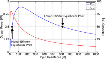
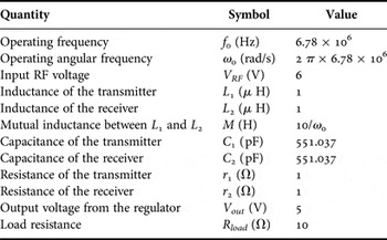
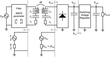
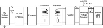
In this section, the problem caused by a receiver-side switching voltage regulator is clarified. The problem is related to a stable operating point. Figure 1 shows an analytical model with a receiver-side switching voltage regulator. First, the determination mechanism of its input resistance value R sr is discussed. Here, the operating frequency f 0 is 6.78 MHz, and both the transmitting resonator and the receiving resonator have the same resonant frequency, i.e.
 $$\omega _0 = \displaystyle{1 \over {\sqrt {L_{\rm 1}C_{\rm 1}}}} = \displaystyle{1 \over {\sqrt {L_{\rm 2}C_{\rm 2}}}}, $$
where ω
0 is the operating angular frequency of 2πf
0. For example, let us consider the input resistance value R
sr
with the parameters listed in Table 1. Figure 2 shows the output power P
rcv
from the rectifier and transfer efficiency η
wpt
as a function of the input resistance value R
sr
of the switching voltage regulator, where P
rcv
is defined as V
rec
I
rec
, P
in
is the output power from an radiofrequency (RF) power source V
RF
, P
load
is the power consumption of the load (calculated as
 $V_{out}^2 /R_{load}$
), and η
wpt
is defined as P
load
/P
in
. In the fundamental analysis described in this section, the rectifier and switching voltage regulator are assumed to be ideal, whereas the analysis described in Section III takes their losses into account. The rectifier was modeled as an ideal full-bridge rectifier. Therefore, it is assumed that
 $$R_{rec} = \displaystyle{8 \over {\pi ^2}}R_{sr}$$
and that the operation of the rectifier is lossless. The input power P sr (=V rec I sr ) to the switching voltage regulator is calculated using the power efficiency η sr of the switching voltage regulator as
 $$P_{sr} = \displaystyle{{V_{out}^2} \over {\eta _{sr}R_{load}}}.$$
General block diagram of a wireless power transfer system with a receiver-side switching voltage regulator.

Output power P rcv from the rectifier and transfer efficiency η wpt as a function of the input resistance value R sr of the switching voltage regulator.

Parameters used in the analysis and simulation.

In this section, the loss in the switching voltage regulator is ignored and η sr is assumed to be 1. At a stable operating point, the output power from the rectifier must be equal to the input power to the switching voltage regulator, i.e.,
 $$P_{rcv} = P_{sr}$$
must be satisfied. Note that (4) represents an equilibrium condition. Because P sr is 52/10 = 2.5 [W], there are two equilibrium points, and their input resistance value R sr that satisfies (4) is approximately 25.3 or 613.8 Ω according to Fig. 2. The efficiency with R sr of 25.3 Ω is much higher than that with R sr of 613.8 Ω.
The stability of each equilibrium point was investigated. At a stable operating point, even if the output voltage V rec changes from the equilibrium voltage V blnc to V blnc + ΔV, V rec (=V blnc + ΔV) must return to V blnc . Hence, when V rec increases from the equilibrium voltage V blnc to V blnc + ΔV, P rcv − P sr must be less than zero so that V rec returns to the equilibrium voltage V blnc , i.e.,
 $$\displaystyle{{d(P_{rcv} - P_{sr})} \over {dV_{rec}}} \lt 0.$$
If d(P rcv − P sr )/dV rec is positive, V rec cannot remain at the equilibrium voltage V blnc . When V rec increases from V blnc to V blnc + ΔV, V rec increases further as d(P rcv − P sr )/dV rec > 0. In the same way, when V rec decreases from V blnc to V blnc − ΔV, V rec decreases further. This implies that an equilibrium point with d(P rcv − P sr )/dV rec > 0 is an unstable equilibrium point. Hence, (5) represents the stability condition. Here, we wish to point out that (5) is true even in the case of losses in the rectifier and switching voltage regulator, because the derivation of (5) does not assume lossless operation.
Based on the assumption that the rectifier and switching voltage regulator are ideal, let us judge the stability of each equilibrium point. Equation (5) can be represented using R sr instead of V rec as
 $$\displaystyle{{d(P_{rcv} - P_{sr})} \over {dR_{sr}}} \lt 0,$$
because dR sr /dV rec is positive with a constant η sr . Since P sr is 2.5 W regardless of V rec , dP sr /dR sr = 0. Further, (6) can be simplified into
 $$\displaystyle{{dP_{rcv}} \over {dR_{sr}}} \lt 0.$$
According to Fig. 2, the equilibrium point with R sr of 613.8 Ω satisfies (7), whereas the other equilibrium point with R sr of 25.3 Ω does not. Thus, the actual value of R sr is 613.8 Ω.
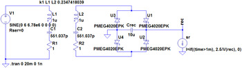
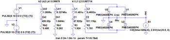
To verify the analysis presented above, we conducted a circuit simulation. Figure 3 shows the circuit simulation setup using LTspice. The components used in the simulation were the same as those used in the analysis except for the rectifier and the switching voltage regulator. The rectifier was modeled as a full-bridge rectifier using four Schottky diodes (PMEG4020EPK) and a smoothing capacitor of 10 μ F. Because the input power to the switching voltage regulator is 2.5 W regardless of V rec , the switching voltage regulator and the load resistance of 10 Ω can be modeled as a component that consumes 2.5 W regardless of V rec . In the simulation on LTspice, the switching voltage regulator and load were modeled as a behavioral current source of 2.5/V rec A. Its power consumption was V rec × 2.5/V rec = 2.5 W. Further, the behavioral current source was activated 1 ms after the initiation of the simulation, so that it could store sufficient energy before starting itself up.
Simulation setup in LTspice.

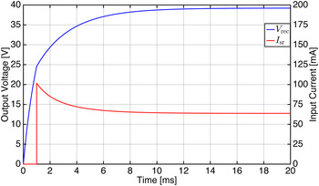
Figure 4 shows the simulated V rec and the input current I sr to the switching voltage regulator, which was simulated as the input current to the behavioral current source. The voltage V rec and input current I sr converged to approximately 39.22 V and 63.8 mA, respectively. Hence, the simulated input resistance value R sr at the stable operating point was approximately 39.22/0.638 ~ 615 Ω, which was close to 613.8 Ω. Thus, the simulation result supports the analysis.
Simulated output voltage V rec from the rectifier and input current I sr to the switching voltage regulator.

The input resistance value R sr of the switching voltage regulator is determined on the basis of (4) and (7). Depending on the input power P sr to the switching voltage regulator, the input resistance values R sr of the equilibrium points also change. However, according to (7) and Fig. 2, the input resistance value R sr cannot be less than the resistance value R sr(mpp) that maximizes the output power P rcv from the rectifier because dP rcv /dR sr is positive when R sr is less than R sr(mpp). Because the output power P rcv is maximized when R rec is equal to
 $$R_{rec{\rm (}mpp{\rm )}} = \displaystyle{{{(\omega M)}^2} \over {r_1}} + r_2,$$
the resistance value R sr(mpp) is calculated as
 $$R_{sr{\rm (}mpp{\rm )}} = \displaystyle{{\pi ^2} \over 8}\left( {\displaystyle{{{(\omega M)}^2} \over {r_1}} + r_2} \right){\rm \sim} 124.6$$
using (2). On the other hand, the resistance value R sr(mep) that maximizes the transfer efficiency η wpt is calculated as
 $$R_{sr{\rm (}mep{\rm )}} = \displaystyle{{\pi ^2} \over 8}r_2\sqrt {1 + \displaystyle{{{(\omega M)}^2} \over {r_1r_2}}} {\rm \sim} 12.4$$
on the basis of (2) and [Reference Awai and Ishizaki10]. With the parameters listed in Table 1, R sr(mpp) is much larger than R sr(mep). Hence, WPT at the maximum efficiency point is impossible. In general, R sr(mpp) is larger than R sr(mep) unless (ωM)2 is equal to 0 because
 $$R_{sr{\rm (}mpp{\rm )}}^2 - R_{sr{\rm (}mep{\rm )}}^2 = \displaystyle{{\pi ^4} \over {64}}\left( {\displaystyle{{{(\omega M)}^4} \over {r_1^2}} + \displaystyle{{r_2{(\omega M)}^2} \over {r_1}}} \right).$$
Thus, the maximum efficiency point, where R sr is R sr(mep), is beyond the stable operating range. Within the stable operating range, the input resistance value of the switching voltage regulator is larger than R sr(mpp), and the transfer efficiency η wpt decreases monotonically as the input resistance value R sr increases according to Fig. 2. Hence, the transfer efficiency η wpt at the stable operating point is less than
 $$\eta _{wpt} \lt \displaystyle{{R_{rec(mpp)}} \over {R_{rec(mpp)} + r_2}} \times \displaystyle{{{{{(\omega M)}^2} / {R_{rec(mpp)} + r_2}}} \over {({{{(\omega M)}^2} / {R_{rec(mpp)} + r_2}}) + r_1}}$$
 $${\hskip-4pt}= \displaystyle{{({(\omega M)}^2/r_1) + r_2} \over {({(\omega M)}^2/r_1) + 2r_2}} \times \displaystyle{{({(\omega M)}^2/({(\omega M)}^2/r_1) + 2r_2)} \over {({(\omega M)}^2/({(\omega M)}^2/r_1) + 2r_2) + r_1}}$$
 $$= \displaystyle{{{(\omega M)}^2/r_1r_2} \over {2(({(\omega M)}^2/r_1r_2) + 2)}}$$
 $$= \displaystyle{{Q_1Q_2} \over {2(Q_1Q_2 + 2)}},$$
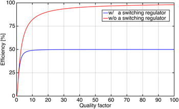
where Q 1 and Q 2 are quality factors defined as ωM/r 1 and ωM/r 2, respectively. Even if Q 1 and Q 2 are high, the maximum efficiency at the stable operating point with a switching voltage regulator is <50% according to (15). With the parameters listed in Table 1, the theoretical and simulated values of η wpt are only 16.2 and 17.7%, respectively. On the other hand, the transfer efficiency at the maximum efficiency point without the receiver-side switching voltage regulator is known to be
 $$\eta _{wpt} = \displaystyle{{Q_1Q_2} \over {{\left( {1 + \sqrt {1 + Q_1Q_2}} \right)}^2}}$$
according to [Reference Awai and Ishizaki10]. The theoretical maximum efficiency with the parameters listed in Table 1 is 81.9%. Figure 5 shows the theoretical maximum efficiencies with and without a receiver-side switching voltage regulator as a function of a quality factor Q = Q 1 = Q 2. As the quality factor increases, the theoretical maximum efficiency without a switching regulator approaches 100%. However, the maximum efficiency with a switching regulator cannot exceed 50%.
Comparison between the theoretical efficiencies with and without a receiver-side switching voltage regulator. Each efficiency is plotted as a function of a quality factor Q = Q 1 = Q 2.

To realize high-efficiency WPT, the input resistance value R sr(mep) should be in the stable operating range. If R sr(mpp) is less than R sr(mep), then R sr(mep) is in the stable operating range. The next section describes a system design using a K-impedance inverter to decrease R sr(mpp).
III. STABILIZATION OF THE MAXIMUM EFFICIENCY POINT
This section discusses the stability condition that takes into account the losses in the rectifier and switching voltage regulator. In addition, it describes a system design using a K-impedance inverter to realize stable operation at the maximum efficiency point. Figure 6 shows an analytical model with an output filter inserted between the RF power source and the transmitting resonator. By inserting an appropriate output filter, we aim to stabilize the input resistance value of R sr(mep), which does not change if there is a slight loss in the output filter.
System configuration with an output filter connected to the output of a power source.

The stability of the input resistance value R sr is determined by (5) even in the case of losses in the rectifier and switching voltage regulator, because the derivation of (5) is not based on the lossless conditions of the rectifier and regulator. However, it is difficult to design the output filter directly from (5). For designing a suitable output filter, it is necessary to represent (5) by using the ABCD-matrix of the output filter and variables in the equivalent circuit shown in Fig. 6.
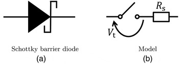
In the analysis, the rectifier was assumed to be a full-bridge rectifier with four Schottky barrier diodes. It is known that a full-bridge rectifier can be precisely analyzed by modeling each Schottky barrier diode as an ideal switch with a voltage drop V
t
equal to the barrier height of the diode and a series resistance R
s
, as shown in Fig. 7 [Reference Ito21]. Assuming a sinusoidal current input of I to the full-bridge rectifier, the input voltage
 $V_{rec\_in}$
to the rectifier is represented as
 $$V_{rec\_in} = \displaystyle{4 \over \pi} (V_{rec} + 2V_t)\displaystyle{I \over {\left \vert I \right \vert}} + 2R_sI.$$
Modeling of a Schottky barrier diode using an ideal switch with the voltage drop V t equal to its barrier height and a series resistance R s .

By applying Kirchhoff's voltage law (KVL), we get
 $$V_{eq} = I(R_{eq} + jX_{eq}) + \displaystyle{4 \over \pi} (V_{rec} + 2V_t)\displaystyle{I \over {\left \vert I \right \vert}} + 2R_sI,$$
where V eq and R eq + jX eq are the equivalent voltage and impedance of Thévenin's equivalent circuit, respectively. Calculating the square of the absolute value of each side gives
 $$\left( {R_{sum}^2 + X_{eq}^2} \right)\left \vert I \right \vert ^2 + 2V_{sum}R_{sum}\left \vert I \right \vert + \left( {V_{sum}^2 - {\left \vert {V_{eq}} \right \vert} ^2} \right) = 0,$$
where V sum and R sum are defined as 4(V rec + 2V t )/π and R eq + 2R s , respectively. Hence, | I| can be solved as
 $$\left \vert I \right \vert = \displaystyle{{ - V_{sum}R_{sum} + \sqrt {{\left \vert {V_{eq}} \right \vert} ^2R_{sum}^2 - \left( {V_{sum}^2 - {\left \vert {V_{eq}} \right \vert} ^2} \right)X_{eq}^2}} \over {R_{sum}^2 + X_{eq}^2}}. $$
The output current I rec from the rectifier is calculated as 2|I|/π, and it is a DC current. Because the output power from the rectifier is calculated as
 $$P_{rcv} = \displaystyle{2 \over \pi} \left \vert I \right \vert V_{rec},$$
dP rcv /dV rec is calculated as follows:
 $$\displaystyle{{dP_{rcv}} \over {dV_{rec}}} = \displaystyle{2 \over \pi} \left \vert I \right \vert - \displaystyle{8 \over {\pi ^2}}V_{rec}\displaystyle{{R_{sum} + V_{sum}X_{eq}^2 /\alpha} \over {R_{sum}^2 + X_{eq}^2}}, $$
where α is given by
 $\sqrt {{\left\vert {V_{eq}} \right\vert}^2R_{sum}^2 - \left( {V_{sum}^2 - {\left\vert {V_{eq}} \right\vert}^2} \right)X_{eq}^2} $
. Hence, (5) is represented as
 $$\displaystyle{2 \over \pi} \left \vert I \right \vert - \displaystyle{8 \over {\pi ^2}}V_{rec}\displaystyle{{R_{sum} + V_{sum}X_{eq}^2 /\alpha} \over {R_{sum}^2 + X_{eq}^2}} - \displaystyle{{dP_{sr}} \over {dV_{rec}}} \lt 0.$$
Here, we consider the stability condition of the equilibrium point where (4) is satisfied. From (4), (20), and (21),
 $$\left \vert I \right \vert = \displaystyle{{ - V_{sum}R_{sum} + \alpha} \over {R_{sum}^2 + X_{eq}^2}} = \displaystyle{{\pi P_{sr}} \over {2V_{rec}}}$$
holds. Further, (23) is transformed into
 $$\eqalign{& \displaystyle{{P_{sr}} \over {V_{rec}}} - \displaystyle{8 \over {\pi ^2}}V_{rec} \cr & \quad \displaystyle{{R_{sum} + \left( {{{V_{sum}X_{eq}^2} / {V_{sum}R_{sum} + \left( {R_{sum}^2 + X_{eq}^2} \right)(\pi P_{sr}/2V_{rec})}}} \right)} \over {R_{sum}^2 + X_{eq}^2}} \cr & \qquad \lt \displaystyle{{dP_{sr}} \over {dV_{rec}}}.}$$
Finally, (25) is simplified into
 $$- \displaystyle{8 \over {\pi ^2}}\left( {\displaystyle{{1 + \beta R_{sum}} \over {R_{sum} + \beta \left( {R_{sum}^2 + X_{eq}^2} \right)}}} \right) \lt \displaystyle{{dI_{sr}} \over {dV_{rec}}},$$
where β is defined as πP sr /(2V sum V rec ). In the last transformation,
 $$\displaystyle{{dI_{sr}} \over {dV_{rec}}} = \displaystyle{d \over {dV_{rec}}}\left( {\displaystyle{{P_{sr}} \over {V_{rec}}}} \right) = \displaystyle{1 \over {V_{rec}}}\displaystyle{{dP_{sr}} \over {dV_{rec}}} - \displaystyle{{P_{sr}} \over {V_{rec}^2}} $$
was applied. By measuring all the variables in (26) around the maximum efficiency point, it is possible to judge whether the maximum efficiency point is stable. However, a system design using (26) is not straightforward.
To realize an easier system design, we propose the use of the sufficient condition of (26) instead of (26) itself. By ignoring
 $$\displaystyle{{\left( {V_{sum}X_{eq}^2} \right)} \over {\left( {V_{sum}R_{sum} + \left( {R_{sum}^2 + X_{eq}^2} \right)(\pi P_{sr}/2V_{rec})} \right) \ge 0}}$$
in (25),
 $$- \displaystyle{8 \over {\pi ^2}}\left( {\displaystyle{{R_{sum}} \over {R_{sum}^2 + X_{eq}^2}}} \right) \lt \displaystyle{{dI_{sr}} \over {dV_{rec}}}$$
is derived as a sufficient condition. Using this inequality is beneficial because the switching voltage regulator can be independently evaluated. The right-hand side does not include the variables of the filter, resonators, or rectifier. Moreover, the left-hand side does not include the variables of the switching voltage regulator. The left-hand side of (28) decreases as |X eq | and R sum approaches 0 and |X eq |, respectively. Because R sum is positive owing to R s , the left-hand side of (28) is minimized when |X eq | is 0 and R sum is minimized. The output filter should be designed to realize sufficiently small values of R sum and |X eq | in order to satisfy (28) in the operating range including the maximum efficiency point. We wish to point out that (28) is equivalent to (26) when |X eq | is 0, because
 $$\displaystyle{{\left( {V_{sum}X_{eq}^2} \right)} \over {\left( {V_{sum}R_{sum} + \left( {R_{sum}^2 + X_{eq}^2} \right)(\pi P_{sr}/2V_{rec})} \right)}}$$
is also 0 when |X eq | is 0. Hence, the sufficient condition (28) approaches the original inequality (26) as |X eq | decreases.
In this paper, we propose the use of a K-impedance inverter as an effective filter. Because R sum and X eq are calculated as
 $$R_{sum} = Re\left( {\displaystyle{{{(\omega M)}^2} \over {(B/A) + r_1}}} \right) + r_2 + 2R_s,$$
 $$X_{eq} = Im\left( {\displaystyle{{{(\omega M)}^2} \over {(B/A) + r_1}}} \right)$$
by using the ABCD-matrix of the output filter and the parasitic resistance values in the resonators shown in Fig. 6, an output filter with sufficiently large |B/A| is necessary.
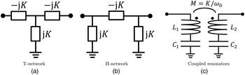
As an output filter with an extremely large |B/A|, a K-impedance inverter is one solution. A K-impedance inverter can be realized by a T-network, a Π-network, or coupled resonators, as shown in Fig. 8. Its function is to convert the impedance of Z into K 2/Z. It has been used to analyze or design the coupling between resonators in WPT [Reference Awai and Ishizaki10, Reference Dionigi and Mongiardo22, Reference Ean, Chuan, Imura and Hori23]. The ABCD-matrix of a K-impedance inverter is represented as
 $$F = \left[ {\matrix{ 0 & { - jK} \cr {\displaystyle{1 \over {jK}}} & 0 \cr}} \right].$$
Examples of circuit configurations of a K-impedance inverter. (a) T-network, (b) Π-network, (c) Coupled resonators whose resonant frequencies are equal to the operating frequency f
0 (
 $f_0 = 1/(2\pi \sqrt {L_1C_1} ) = 1/(2\pi \sqrt {L_2C_2} $
).

Hence, |B/A| is infinity. When |B/A| is infinity, R sum = r 2 + 2R s and X eq = 0. Then, (28) can be converted into
 $$- \displaystyle{8 \over {\pi ^2\left( {r_2 + 2R_s} \right)}} \lt \displaystyle{{dI_{sr}} \over {dV_{rec}}}.$$
Note that (32) represents the limitation of the proposed method. The proposed method is not effective for combinations of devices that do not satisfy (32).
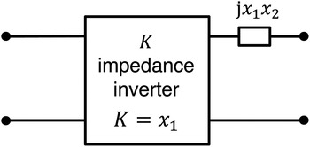
Besides the K-impedance inverter, there are other filters with large |B/A|. However, the advantaged of the K-impedance inverter is that it does not affect the power factor. When the impedance seen from the input of the transmitter is purely resistive, the input impedance of the K-impedance inverter is also purely resistive. On the other hand, there is an alternative way to design an output filter that consists only of reactance elements to minimize the loss in the filter. Because A of the ABCD-matrix should be 0 to realize large |B/A|, the ABCD-matrix of the filter with only reactance elements can be represented as
 $$F = \left[ {\matrix{ 0 & { - jx_1} \cr {\displaystyle{1 \over {jx_1}}} & {x_2} \cr}} \right],$$
where x 1 and x 2 are real numbers. For example, the output filter with the ABCD-matrix of (33) can be realized using a K-impedance inverter with K = x 1 and a lumped reactance element with an impedance of j x 1 x 2, as shown in Fig. 9.
Realization of (33) with a K-impedance inverter of K = x 1 and a lumped reactance element with its impedance of j x 1 x 2.

To verify the effectiveness of the K-impedance inverter, we conducted a circuit simulation. The components were the same as those presented in Section II except for the insertion of a K-impedance inverter with K = 10. The K-impedance inverter was modeled using a T-network circuit including two series inductors of 234.7 nH and a shunt capacitor of 2.347 nF. The simulated V
rec
, I
sr
, and η
wpt
were 2.586 V, 967 mA, and 52.2%, respectively. The R
sr
value of the operating point was just
 $2.586/0.967{\rm \sim} 2.67{\kern 1pt} \,\Omega $
, which was smaller than R
sr(mep). Thus, the maximum efficiency point was in a stable operation range. However, to maximize the transfer efficiency, R
sr
should be adjusted to R
sr(mep). The next section describes an efficiency maximization method based on input voltage control.
IV. MAXIMIZING EFFICIENCY BY INPUT VOLTAGE ADJUSTMENT
Recently, a maximum efficiency point tracking method using a receiver-side DC–DC converter has been studied extensively. A switching voltage regulator is a type of DC–DC converter, but it is impossible to control its duty ratio to maximize efficiency because the duty ratio is controlled to regulate the output voltage. However, the duty ratio depends on the ratio of V
out
and V
rec
. Moreover, V
rec
depends on the input voltage V
RF
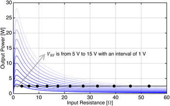
. Here, maximum efficiency point tracking is realized by controlling the duty ratio indirectly via input voltage control. Figure 10 shows the theoretical output power P
rcv
from the rectifier when the input voltage V
RF
varies from 5 to 15 V. As the input voltage V
RF
increases, the input resistance value of the stable operating point denoted by a black circle also increases. Figure 11 shows the simulated R
sr
and transfer efficiency η
wpt
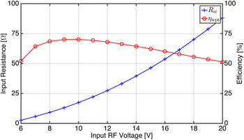
with a K-impedance inverter of a T-network circuit including two inductors of 234.7 nH and a capacitor of 2.347 nF. As the input voltage value V
RF
increases, the input resistance R
sr
also increases in the simulation. Depending on the change in R
sr
, the transfer efficiency η
wpt
has one peak. When the input voltage V
RF
is around 10 V, the transfer efficiency is maximized (70.1%) and R
sr
is 17.4 Ω. These results validate the proposed efficiency maximization based on input voltage control with the switching voltage regulator. By monitoring the output power from the RF power source (P
in
) while changing its voltage value V
RF
, the input voltage value V
RF(opt) that minimizes the output power P
in
can be obtained. Further, V
RF(opt) is the optimum input voltage value of the RF power source V
RF
because the power consumption of the load is
 $V_{out}^2 /R_{load}$
, which is a constant. The simulated optimum R
sr
of 17.4 Ω is larger than the theoretical R
sr(mep), which is 12.4 Ω. The difference is attributed to the losses in the rectifier. In general, the power conversion efficiency of the rectifier increases with V
rec
. Thus, higher R
sr
enhances the efficiency of the rectifier. The proposed efficiency maximization is effective in enhancing the efficiency of both the coupled resonators and the rectifier. We note that the maximum efficiency realized by the proposed method is slightly lower than that realized by conventional DC–DC converter-based methods because the K-impedance inverter has a small loss. However, as described in Section V, the efficiency of the K-impedance inverter is virtually negligible. In the experiments described in Section V, the efficiency is more than 97.5%.
Output power P rcv as a function of the input resistance value R sr in a system with a K-impedance inverter of K = 10 when the input voltage value V RF is from 5 to 15 V.

Simulated transfer efficiency η wpt and output voltage V rec as a function of the input voltage value with a K-impedance inverter of K = 10.

V. MEASUREMENTS AND SIMULATIONS
To confirm the validity of the proposed methods, we implemented a WPT system with a K-impedance inverter and conducted experiments at an operating frequency of 6.78 MHz. In addition, circuit simulations using LTspice were conducted with the measured parameters of the fabricated devices, and the results were compared with measurement results.
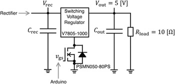
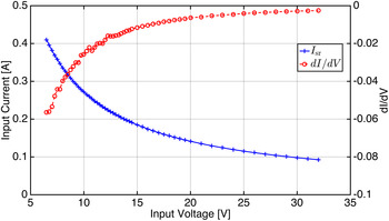
In the measurements and simulations, the output voltage of the switching voltage regulator was 5 V and the load resistance was 10 Ω, assuming power supply to USB 1.x and 2.0 devices in a desktop environment. The voltage rating of USB 1.x and 2.0 devices is 5 V, while their power limitation is 2.5 W. Further, 10 Ω is the load resistance required to consume 2.5 W. As the switching voltage regulator and load of 10 Ω, V7805-1000 (CUI Inc.) and LN-300A-G7 (KEISOKU GIKEN) were used, respectively. In this study, the off-the-shelf switching voltage regulator V7805-1000 was utilized. We believe that an off-the-shelf switching voltage regulator is useful because it facilitates the design and fabrication of power-receiving devices. According to the data sheet of V7805-1000, its input voltage ranges from 6.5 to 32 V, the maximum output current is 1 A, and the power conversion efficiency ranges from 88 to 93%. An n-channel MOSFET (PSMN050-80PS) was inserted as shown in Fig. 12 to activate V7805-1000 after storing sufficient energy in C rec to activate it. The drain–gate voltage v ds was controlled using Arduino MEGA. Further, the V–I characteristics of the switching voltage regulator were measured using a power analyzer (Hioki E.E. Corp. PW6001) and a DC power supply (TDK-Lambda Z60-7) in a constant voltage mode, as shown in Fig. 13. Based on the measured values, the range of the input resistance value was calculated as around 12–100 Ω. In addition, dI sr /dV rec , which is the right-hand side of (28), was calculated numerically, as shown in Fig. 13; its minimum value is approximately −0.0565. Hence, if the left-hand side of (28) is less than −0.0565, any input voltage from 6.5 to 32 V is in the stable operating range.
Connection between V7805–1000 and the load of 10 Ω. An MOSFET is inserted for enabling or disabling the switching voltage regulator.

Measured input current to V7805–1000 and the right-hand side of (29) as a function of the input voltage value.

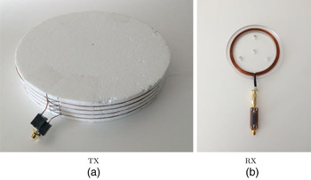
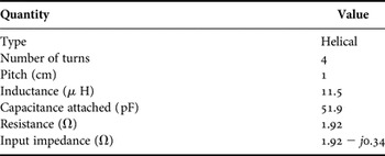
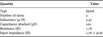
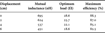
Figure 14 shows the fabricated transmitting resonator and receiving resonator. Both consist of copper wire having a diameter of 1 mm. As the capacitors, polypropylene film capacitors of the KEMET R73 or R74 series were used. The transmitting resonator was a helical coil around a polystyrene foam core, having 4 turns, a diameter of 30 cm, and a pitch of 1 cm; it was connected in series with a capacitor of 62.2 pF. Further, its input impedance was 1.92 − j0.34 Ω. The receiving resonator was a spiral coil around an acrylic plate, having five turns and an inner diameter of 10 cm; it was connected in series with a capacitor of 100 pF. Further, its input impedance was 1.78 + j0.67 Ω. The parameters of the resonators are listed in Tables 2 and 3. In the measurements, the vertical displacement of the receiving resonator was 0, 2, 4, and 6 cm from the top of the transmitting resonator. By using the measured mutual inductances and the parasitic resistance of each resonator, we calculated the optimum input resistance value R rec of the rectifier on the basis of [Reference Awai and Ishizaki10]. The measured mutual inductance, optimum input resistance value R rec , and theoretical maximum efficiency with each vertical displacement are listed in Table 4. From the optimum value of R rec , the optimum input resistance value R sr of the switching regulator was calculated as 23.2, 20.8, 17.9, and 15.1 Ω by using (2). All these values are in the range of the input resistance value of V7805-1000.
Fabricated resonators: (a) transmitter and (b) receiver.

Parameters of the fabricated transmitting resonator.

Parameters of the fabricated receiving resonator.

Mutual inductances, optimum resistances, and theoretical maximum efficiencies.

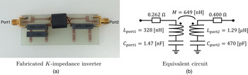
To stabilize the maximum efficiency point, a K-impedance inverter was fabricated. In this measurement, the K-impedance inverter was fabricated using coupled resonators as shown in Fig. 8(c). The optimum resistance value for minimizing the loss in the K-impedance inverter using coupled resonators can be calculated in the same way as that for WPT because their configurations are the same. Figure 15(a) shows the K-impedance inverter fabricated using a ferrite core (EPCOS B62152A1X1). Fig. 15(b) shows the equivalent circuit and measured parameters. Because the input impedance Z in seen from the input of the transmitting resonator when R rec is optimum can be calculated as
 $$\eqalign{Z_{in} & = r_1 + \displaystyle{{{(\omega M)}^2} \over {r_2 + R_{rec(mep)}}} \cr & = r_1 + \displaystyle{{{(\omega M)}^2} \over {r_2 + r_2\sqrt {1 + ({(\omega M)}^2/r_1r_2)}}},}$$
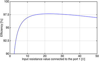
the theoretical values of Z in with vertical displacements of 0, 2, 4, and 6 cm are 30.8, 27.7, 23.9, and 20.1 Ω, respectively. It is important to design a highly efficient K-impedance inverter with an input impedance of 20.1–30.8 Ω. Their average value is approximately 25.6 Ω. We adjusted the number of turns of each inductor such that the input resistance value for minimizing the loss in the K-impedance inverter would be close to 25.6 Ω. As a result, the number of turns of the inductor connected to port 1 was one and the number of turns of the other inductor was two. When the RF power source was connected to port 1 of the K-impedance inverter, the optimum impedance connected to port 2 was calculated as 34.2 Ω. On the other hand, when port 2 was connected to the power source, the optimum impedance of port 1 was 22.4 Ω. Hence, port 2 was connected to the RF power source and port 1 was connected to the transmitter. Figure 16 shows the efficiency of the fabricated K-impedance inverter when a resistive load is connected to its port 1. The efficiency was calculated using the measured parameters of the fabricated K-impedance inverter and defined as the power consumption of the resistance connected to port 1 divided by the input power from port 2. From 15 to 33.5 Ω, the efficiency was >97.5%. Hence, the loss in the K-impedance inverter has an insignificant effect on the overall efficiency of the implemented wireless power system. When the range of input impedances is too wide to be covered by a single K-impedance inverter, connecting several K-impedance inverters via switches and activating only one of them is an effective approach. It is noted that a K-impedance inverter should be fabricated with heat sinks when the transferred power is sufficiently high to cause heating of the K-impedance inverter.
Fabricated K-impedance inverter and its equivalent circuit.

Efficiency of the fabricated K-impedance inverter as a function of the input resistance value connected to its port 1.

As the RF power source, a class-D zero voltage switching full-bridge inverter (EPC9065) was used. We used a DC voltage sources (TDK-Lambda Z60-7 and TEXIO PA18-3B) in a constant voltage mode as the main power source and logic supply to EPC9065. A full-bridge rectifier was implemented using PMEG4020EPK diodes, a ceramic capacitor of 10 μ F, and an aluminum electrolytic capacitor of 470 μ F. We measured the equivalent impedance R eq + jX eq by using a vector network analyzer (Rohde & Schwarz ZVL3). During the measurements, port 1 of the K-impedance inverter was connected to the transmitting resonator and port 2 was a short circuit because the output impedance of a class-D inverter can be approximated as 0 Ω [Reference Ishida, Yamaguchi, Ishizaki and Awai24, Reference Awai25]. Table 5 lists the measured values of R eq + jX eq . According to the data sheet of PMEG4020EPK, V t and R s were approximated as 0.395 V and 95 m Ω. Therefore, the left-hand side of (28) can be calculated as −0.307, −0.339, −0.371, and −0.400 with vertical displacements of 0, 2, 4, and 6 cm, respectively. The maximum value of the left-hand side of (28) was −0.307; hence, the value of the left-hand side was always less than the minimum value of the right-hand side of (28) at any vertical displacement. Thus, the overall input voltage of the switching voltage regulator is in the stable operating range, as is the maximum efficiency point.
Measured value of R eq + jX eq with vertical displacements.

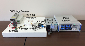
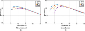
Figure 17 shows the measurement setup, and the block diagram of the measurement setup is shown in Fig. 18. Figure 19 shows the simulation setup. In the simulations, an RF power source was modeled using two square-wave voltage sources having a duty ratio of 50%. The switching regulator was also modeled as a behavioral current source of 2.5/0.9 W, assuming that the power conversion efficiency of the switching voltage regulator was 90%. Figure 20(a) shows the measured efficiency η meas . The measured efficiency η meas was defined as the power consumption P out of the load of 10 Ω divided by the input power P in from a constant DC voltage source. Hence, η meas includes the efficiencies of the DC–RF inverter, K-impedance inverter, coupled resonators, rectifier, and switching voltage regulator. The minimum input voltage V in , which is defined in Fig. 18, with each vertical displacement was the value when V rec reached 6.5 V. Figure 20(b) shows the simulated efficiency η sim , which was defined as 2.5 W divided by the total output power from two square-wave voltage sources. The input voltage V in was varied from 1 to 30 V at intervals of 1 V. The simulated efficiency was shown with the input voltage V in that realized a power supply of 2.5 W. Both the simulation results and the measurement results showed that the efficiency curve as a function of the input voltage V in with each vertical displacement has one peak and the peak efficiency is >50%, although the theoretical maximum efficiency without a suitable output filter does not reach 50%. Thus, the maximum efficiency point is successfully stabilized by the K-impedance inverter, and the transfer efficiency can be maximized by applying input voltage adjustment. Moreover, the fabricated WPT system could realize stable operation even when V rec is equal to 6.5 V. Hence, the entire range of the input voltage to the switching regulator was stabilized. The proposed methods were thus validated by both measurements and simulations. There are voltage gaps of about 2 V between the input voltage values (V in ) to maximize the efficiency in the simulations and measurements, which are attributed to errors caused by modeling of the diodes, rectifier, RF power source, and switching voltage regulator in the simulations. The rectifier may cause errors owing to the parasitic resistance, capacitance, and inductance in the printed circuit board as well as individual differences in the Schottky barrier diodes employed in the rectifier. Two square-wave voltage sources were used to model the full-bridge class-D inverter; hence, the losses in the field effect transistors (FETs) and the effect of dead time were not considered in the simulations. The efficiency of the switching voltage regulator was assumed to be 90% in the simulations; however, the actual value varies between 88 and 93% depending on the input voltage to the regulator.
Experimental setup.

Block diagram of experimental setup.

Simulation setup for the verification of measurement results.

Measured efficiency η meas and simulated efficiency η sim as a function of the input voltage V in to a class-D inverter when the vertical displacement of the receiver is 0, 2, 4, and 6 cm.

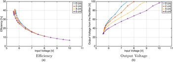
We also tried to transmit power without the K-impedance inverter, but it was impossible within the recommended current limitations of EPC9065 and the operation range of the input voltage of V7805-1000. This is because when R sr is larger than R sr(mpp), the input impedance seen from the input of the transmitting resonator is less than 2r 1 in a system without the K-impedance inverter, and a larger value of R sr requires a larger output voltage V rec to consume 2.5 W. Instead, we simulated the transfer efficiency without a K-impedance inverter. Figure 21(a) shows the simulated transfer efficiency as a function of the input voltage of the RF power source. The full-bridge rectifier was originally modeled with Schottky diodes (PMEG4020EPK); however, we used PMEG10020ELR in this simulation, because it was found that the output voltage V rec exceeded 40 V in most of the simulation conditions, as shown in Fig. 21(b). The input voltage was varied at intervals of 0.01 V to find the minimum input voltage for realizing a power supply of 2.5 W. As the input voltage decreases to the minimum input voltage, the efficiency increases monotonically, but it does not reach 50%. This result supports the theoretical analysis and confirms the effectiveness of the K-impedance inverter.
Simulated efficiency η sim and output voltage V rec from the rectifier without the K-impedance inverter as a function of the input voltage V in to a class-D inverter.

VI. CONCLUSION
Instead of controlling the frequency or input voltage, using a switching regulator in the receiver side of a WPT system is one of the solutions to realize stable output voltage. However, this paper showed that the receiver-side switching voltage regulator drastically degrades the WPT efficiency because of its input resistance value at a stable operating point. Specifically, the input resistance value at a stable operating point is higher than the optimum resistance value in a WPT system with a class-D inverter and series-resonant transmitter and receiver. To maximize the transfer efficiency, we derived the input resistance value of the switching voltage regulator at a stable operating point, and we proposed a system design with a K-impedance inverter. The system with the receiver-side switching voltage regulator and the K-impedance inverter as an output filter in the RF power source achieved the optimum input voltage for maximizing the transfer efficiency. Simulations and measurements showed the effectiveness of the proposed methods. The proposed method is beneficial for wirelessly powering electric devices that require a constant operating voltage, such as home appliances, mobile phones, and micro-controller boards.
ACKNOWLEDGEMENTS
This work was supported by ERATO (Exploratory Research for Advanced Technology) of JST Strategic Basic Research Programs and a grant-in-aid for JSPS Fellows (26.7147).
 Yoshiaki Narusue received the B.E. and M.E. degrees in Information and Communication Engineering from the Graduate School of Information Science and Technology, The University of Tokyo, Tokyo, Japan, in 2012 and 2014, respectively. Currently, he is pursuing the Ph.D. degree in the same department. He received the second-best student paper award at the IEEE Radio and Wireless Symposium in 2013. His research interests mainly include wireless power transfer using magnetic resonant coupling and energy harvesting from microwaves. Mr. Narusue is a student member of the IEEE, IEICE, and IPSJ.
 Yoshihiro Kawahara received the B.E., M.E., and Ph.D. degrees in Information and Communication Engineering from The University of Tokyo, Tokyo, Japan, in 2000, 2002, and 2005, respectively. Currently, he is an Associate Professor with the Department of Information and Communication Engineering, The University of Tokyo, Tokyo, Japan. He joined the faculty in 2005. From 2011 to 2013, he was a Visiting Scholar with the Georgia Institute of Technology, Atlanta, GA, USA. Further, he was a Visiting Assistant Professor with the Massachusetts Institute of Technology, Cambridge, MA, USA, in 2013. His research interests lie in the areas of computer networks and ubiquitous and mobile computing. He is currently interested in developing energetically autonomous information communication devices. Dr. Kawahara is a member of the IEICE and IPSJ. He also is a committee member of IEEE MTT TC-24 (RFID Technologies).
 Tohru Asami received the B.E. and M.E. degrees in Electrical Engineering from Kyoto University, Kyoto, Japan, in 1974 and 1976, respectively, and the Ph.D. degree in information and communication engineering from The University of Tokyo, Tokyo, in 2005. In 1976, he joined KDD (KDDI), Tokyo, Japan. Since then, he has been working in several research areas such as UNIX-based data communication systems and network management systems. After serving as the CEO of KDDI R&D Laboratories, Inc., he joined the University of Tokyo in 2006 as a Professor with the Department of Information and Communication Engineering, Graduate School of Information Science and Technology. Professor Asami was a Vice Chairman on the Board of Directors of the Information and Systems Society at the Institute of Electronics, Information and Communication Engineers, Japan (IEICE-ISS), from 2003 to 2005.