2.1. Telematics variables

A trip is defined as the period from engine start to engine switch off. During a trip, we receive records from three independent sensors: GPS, instrumental panel, and three-axis accelerometer.

2.2. Telematics data cleaning

Telematics car driving data have a large size and are deemed big data. Data cleaning for such big data is very challenging since the same procedure needs to be applied to all the trips of all cars. Thus, the data cleaning should be adequately flexible for this aim. An investigation using several visual tools implies that we need to consider two data cleaning issues. First, there are missing values in GPS coordinates (x,y), GPS speed $v^{(gps)}$ , GPS heading $\psi^{(gps)}$ , and instrument panel speed $v^{(vss)}$ . These missing values need to be interpolated, respectively. Second, there are frequent calibration issues with the accelerometer variables $a^{(acc)},a'^{(acc)}$ . It is difficult to remove the calibration bias since the timing and severity of such a bias are rather random. Consequently, it is better to consider other variables to describe the acceleration in two directions.

2.2.1. Data imputation

Data imputation is essential if time series of telematics variables are analyzed. On the contrary, if only summary statistics of telematics variables are employed (e.g., mean of speed or standard deviation of acceleration), the interpolation of missing values is not necessary according to the law of large numbers.

In this paper, missing values of GPS coordinates (x,y), GPS speed $v^{(gps)}$ , GPS heading $\psi^{(gps)}$ , and instrument panel speed $v^{(vss)}$ are linearly interpolated, respectively. Note that missing values at boundaries of trips cannot be interpolated, and such missing values are therefore truncated. The imputation of GPS heading $\psi^{(gps)}$ around 0 or 360 degree is challenging and may leads to biased GPS heading imputation. However, such biased imputation should have little effects on angle change due to the useness of sine and arc-sine functions; see Equation (2). Nevertheless, the proportion of missing values in our data set is very small. Thus, we reply on our data quality with high confidence. Please see Figures 1–4 in the supplementary material for details.

Figure 1:

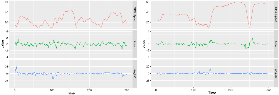
Two sample trips.

Figure 2:

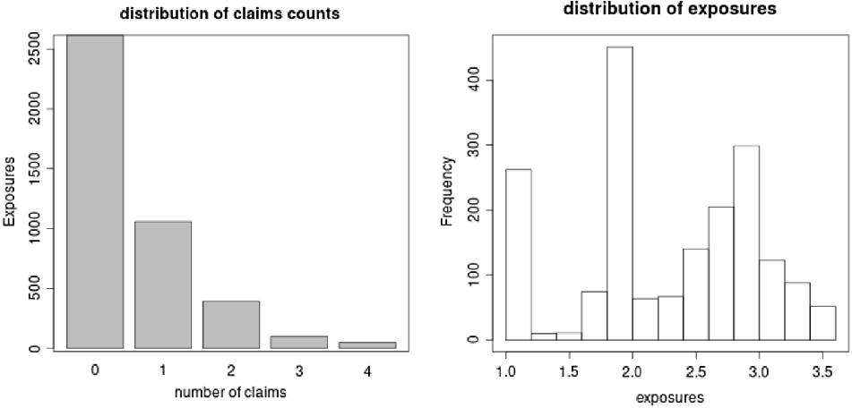
The distributions of claims number and exposures.

Figure 3:

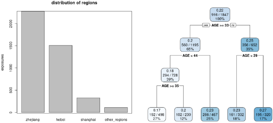
The distribution of exposures across four regions. The marginal Poisson tree with driver’s age covariate.

Figure 4:

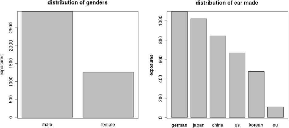
The distribution of exposures across genders. The distribution of exposure across car made countries.

2.2.2. Derived acceleration and angle change

Since the quality of accelerometer variables is relatively questionable, alternative measures are derived to measure the acceleration and direction changes. We derive longitudinal acceleration rates $a^{(gps)}, a^{(vss)}, a^{(xy)}$ from GPS speed $v^{(gps)}$ , instrument panel speed $v^{(vss)}$ , and GPS coordinates (x,y), respectively,

(1) \begin{equation} \begin{aligned} a^{(gps)}_t&=v^{(gps)}_{t}-v^{(gps)}_{t-1} \\[3pt] a^{(vss)}_t&=v^{(vss)}_{t}-v^{(vss)}_{t-1} \\[3pt] a^{(xy)}_t&=v^{(xy)}_{t}-v^{(xy)}_{t-1} \end{aligned},\end{equation}

where

\begin{equation*}v^{(xy)}_t=\sqrt{(x_t-x_{t-1})^2+(y_t-y_{t-1})^2}.\end{equation*}

We replace lateral acceleration $a'^{(acc)}$ by angle changes of heading directions $\Delta^{(gps)},\Delta^{(xy)}$ , which are derived from GPS heading $\psi^{(gps)}$ and GPS coordinates (x,y), respectively,

(2) \begin{equation} \begin{aligned} \Delta^{(gps)}_t&=\arcsin\left( \sin\left(\psi^{(gps)}_{t}-\psi^{(gps)}_{t-1}\right)\right) \\[4pt] \Delta^{(xy)}_t&=\arcsin\left(\sin\left(\psi^{(xy)}_{t}-\psi^{(xy)}_{t-1}\right)\right), \end{aligned}\end{equation}

where

\begin{align*}\psi^{(xy)}_t =\, & \mathbb{1}_{(-\infty,0)}\left(\arctan2\left(\frac{x_t-x_{t-1}}{y_t-y_{t-1}}\right)\right)\times2\pi\\[4pt]& +\arctan2\left(\frac{x_t-x_{t-1}}{y_t-y_{t-1}}\right)\in[0,2\pi].\end{align*}

Note that a positive value of $\Delta$ indicates a right turn whereas a negative one suggests a left turn. The jump between 0 and 360 is not an issue since we take sine values.

2.3. Time series of individual trips

A trip may contain several standing still phases $\{t: v_t=0 ,a_t=0, \Delta_t=0\}$ . Those phases should be removed since they are irrelevant to driving behavior. Also, it is worth noting that GPS variables tend to be more unreliable with a slow driving speed (e.g., when parking). Thus, by focusing on a meaningful and usual speed interval [10,60] km/h, we can make more sensible comparison among drivers. It is worth pointing out that one may consider several speed intervals, for example, [10,60], (60,90], (90,120] km/h, and study partial trips on those speed intervals, respectively. We refrain from attempting this approach since our portfolio is small, and many drivers in downtown have very few trips with speed above 60 km/h in our data set.

We first extract partial trips in [8, 62] km/h and set the acceleration and angle change in the shifting parts $[8,10] \cup [60,62]$ km/h to 0. Further, we truncate speed in the shifting parts $[8,10] \cup [60,62]$ km/h to 10 and 60 km/h, respectively. The first $\tau=5\times60$ s of such concatenated trips are then saved for each trip. If a trip did not spend more than 5 min in speed interval [8,62] km/h, it would be discarded in the analysis.

We extract at most 500 preprocessed trips for each driver. Therefore, for each driver $i=1,\ldots,n$ , we have $c_i\in (0,500]$ individual trips. For driver i, we stack its trips into a $c_i\times300\times3$ array $\textbf{z}_i=(z_{i,1},\ldots,z_{i,c_i})'$ , where each trip $z_{i,j}\in[10,60]^{300}\times[-4,4]^{300}\times[-45^{\circ},45^{\circ}]^{300}$ . Note that the unbolded notation $z_j$ refers to a trip j without considering which driver it belongs to. Two sample trips are plotted in Figure 1, which shows that speeding, braking, and direction changes are always associated with low speed. Note that in Section 4.3, it is demonstrated that stable results can be obtained based on those 500 trips.

Remarks. One may choose the middle stage of a trip to improve data reliability. However, it is difficult to define such a stage. On one hand, for instance, if the middle 5 min were selected, it would be unfair for trips with varying durations. On the other hand, if the first several minutes (e.g., 10 min) were discarded and the next 5 min were selected, it would be not appropriate for short trips (e.g., shorter than 15 min). Therefore, by extracting and focusing on the first 5 min, we fairly compare driving behavior in the early stage of a trip. In addition, we have specified particular speed interval and truncate acceleration and angle change. A particular speed interval makes the comparison among drivers more sensible, and the truncation eliminates leverage effects of outliers. We only focus on the first 5 min of a trip rather than a longer period or the whole trip for two reasons. First, a 1D CNN will be employed to fit the trips which only allows for inputs of the same length. Second, by choosing this short period of trips, we can largely reduce the computational time with limited resource. Admittedly, by using cloud computing and other learning algorithms, one may directly work on the complete trips to further improve the accuracy. This remains for future works.

3.1. General setting of claims frequency modeling

We assume that claims number $N_i$ follows a Poisson distribution with mean of $e_i\lambda(\textbf{x}_i)$

\begin{equation*}N_i \overset{ind}{\sim} \text{Poi} (e_i\lambda(\textbf{x}_i)),\end{equation*}

where $e_i$ is the exposure, and $\lambda(\textbf{x}_i)$ is the claims frequency per driver per year given the risk factors $\textbf{x}_i\in \mathcal{X}$ . The function $\lambda$ is a mapping from risk factors to claims frequency:

\begin{equation*}\lambda: \mathcal{X} \rightarrow \mathbb{R}_+, \textbf{x}\mapsto \lambda(\textbf{x}).\end{equation*}

We first establish the base line generalized linear model (GLM) with $\lambda$ as a log-linear function in this section. Then in Section 4, we improve it by introducing telematics covariates to expand the covariate space $\mathcal{X}$ .

We will compare models in terms of out-of-sample prediction performances. Stratified split (w.r.t. number of claims) is used to partition the data into train $\mathcal{D}_{\text{train}}$ , validation $\mathcal{D}_{\text{validation}}$ , and test data $\mathcal{D}_{\text{test}}$ with a proportion of ( $0.6:0.2:0.2$ ). We denote the corresponding index sets by $\mathcal{I}_{\text{train}}, \mathcal{I}_{\text{validation}}$ , and $\mathcal{I}_{\text{test}}$ , respectively. The exposures, claims counts, and claims frequencies of each data set are listed in Table 1. The index of learning data $\mathcal{D}_{\text{learn}}=\mathcal{D}_{\text{train}}\cup\mathcal{D}_{\text{validation}}$ is denoted by $\mathcal{I}_{\text{learn}}=\mathcal{I}_{\text{train}}\cup\mathcal{I}_{\text{validation}}$ .

Table 1

Data partitions.

It is natural to use the Poisson deviance loss to compare different models. The out-of-sample Poisson deviance loss on the data $\mathcal{D}_{\text{test}}$ is defined as

(3) \begin{equation} \mathcal{L}(\hat{\lambda},\mathcal{D}_{\text{test}})=\frac{2}{|\mathcal{D}_{\text{test}}|}\sum_{i \in \mathcal{I}_{\text{test}}}\left(e_i\hat{\lambda}(\textbf{x}_i) - N_i -N_i \ln e_i\hat{\lambda}(\textbf{x}_i) + N_i\ln N_i \right),\end{equation}

where the estimated mapping $\hat{\lambda}$ contains estimated parameters using the learning data $\mathcal{D}_{\text{learn}}$ .

3.2. Preprocessing classical actuarial risk factors

The available actuarial risk factors are regions, driver’s age, driver’s gender, car brand, car’s age, seat count, car’s price, and average daily distance. For categorical variables, we merge levels containing few exposures. For continuous variables, we investigate their marginal effect on claims frequency and discretize them when necessary. Note that the last covariate average daily distance is obtained from the original telematics data rather than the preprocessed $c_i$ trips defined in Section 2.3. Strictly speaking, this variable is not a classical actuarial risk factor. We include this variable together with other classical actuarial risk factors, since the distance exposure has been studied intensively in actuarial literature and widely used in the usage-based insurance.

Regions. There are three main regions, Hebei Province, Zhejiang Province, and Shanghai City, which have accounted for 97.67% of total cars. Hence, we merge the remaining regions as one, denoted by “other regions”. The distribution of exposures across those four regions is shown in Figure 3. Note that one may create a continuous variable of population density in each region. This variable should be related to claims frequency, since it is a proxy of traffic density.

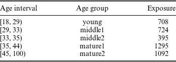
Driver’s age. It is widely acknowledged that driver’s age has a nonlinear relationship with claims frequency. Thus, we discretize driver’s age into five groups according to a marginal Poisson regression tree as shown in Figure 3. The cutoff values of age are 29, 33, 35, and 44. We list driver’s age group and their exposures in Table 2.

Table 2

Driver’s age groups.

Gender. Male drivers are almost twice the size of female drivers as shown in Figure 4.

Car brands. There are 66 different car brands. Due to the small sample sizes of individual car brands, we create a new categorical variable of car made country with 6 levels: Germany, Japan, China, US, Korea, and Europe (excluding Germany). Figure 4 displays the distribution of exposures across car made countries.

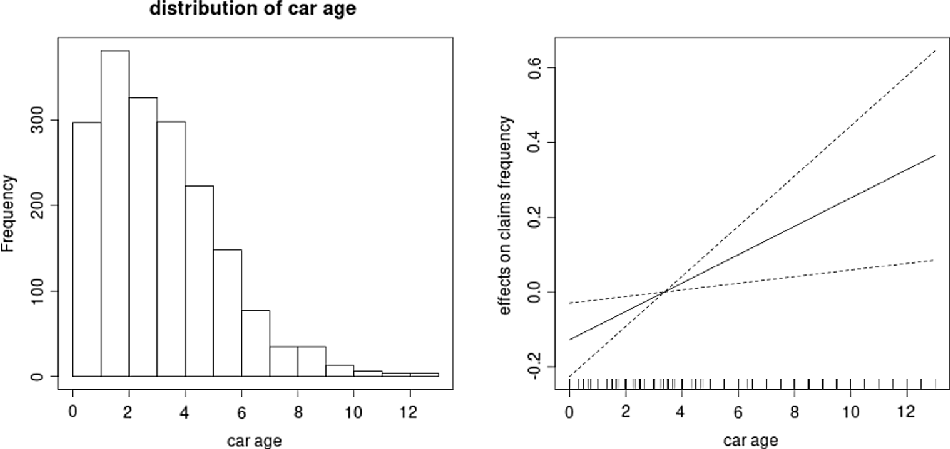
Car’s age. The distribution of car’s age is plotted in Figure 5. A marginal generalized additive model (GAM) for claims frequency indicates that car’s age is related to claims frequency in a log-linear fashion (due to the logarithm link function) as shown in Figure 5. Thus, discretization is not needed for this variable.

Figure 5:

Histogram of car’s age. The effect of car’s age on claims frequency (from a marginal GAM).

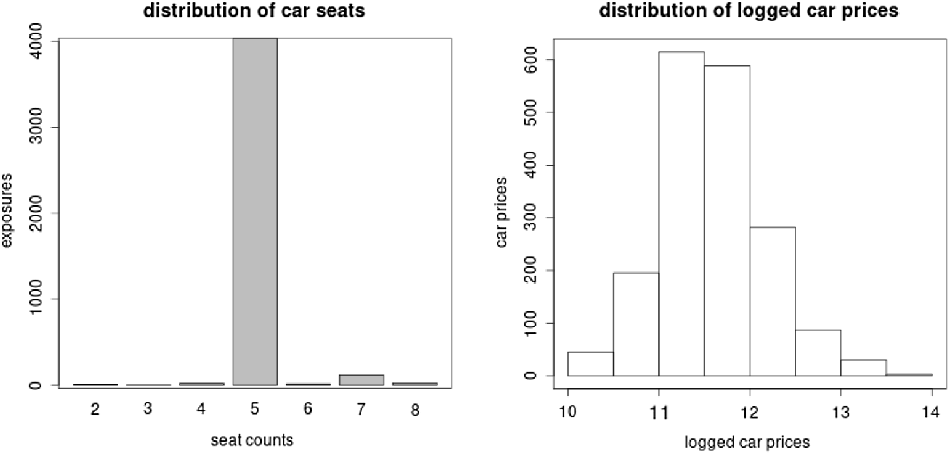
Seat count. Around 95.67% cars have 5 seats as shown in Figure 6. Hence, this variable is not quite useful for claims frequency prediction.

Figure 6:

The distribution of exposure across seat count. Histogram of logged car’s price.

Car’s price. The distribution of car’s price in logarithm is shown in Figure 6. A preliminary analysis (using marginal tree, GAM, and GLM) demonstrates that this variable does not have a close relationship with claims frequency. This may be due to the relative small size $n=1847$ of our portfolio.

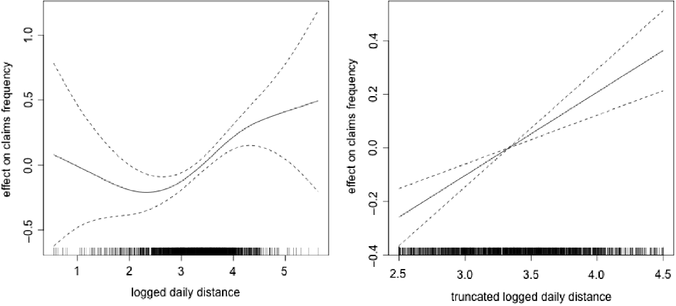
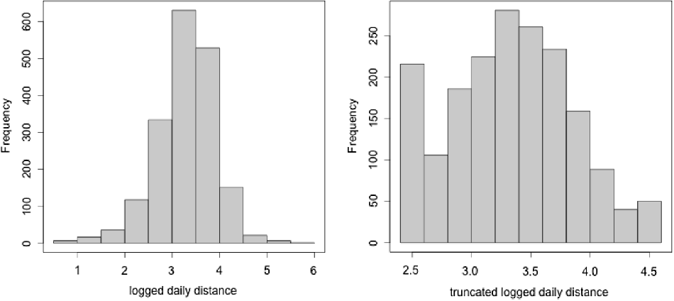
Average daily distance. We fit a marginal GAM to investigate nonlinear effect of average daily distance on claims frequency. The left plot in Figure 7 suggests that the logged daily distance are mainly distributed between 2.5 and 4.5. Thus, we truncate the logged daily distance at 2.5 and 4.5, and re-fit a marginal GAM with truncated values. The right plot in Figure 7 indicates that the truncated logged daily distance is related to claims frequency in a log-linear fashion (due to the logarithm link function). We will then use the truncated and logged average daily distance in GLM. Figure 8 compares the distributions of original and truncated variables.

Figure 7:

The effects of logged daily distance on claims frequency (from two marginal GAMs).

Figure 8:

The distributions of logged daily distance without and with truncation at 2.5 and 4.5.

In summary, we have 4 categorical covariates: regions, driver’s age groups, gender, and car made countries and 2 continuous covariates: car’s age and (truncated and logged) average daily distance. Seat count, and car’s price will not be used in the following analysis.

3.3. Poisson generalized linear models for claims frequency

We begin with the classical generalized linear model (GLM), which assumes the following log-linear mapping:

(4) \begin{equation} \begin{aligned} \ln \lambda^{\text{(GLM)}}(\textbf{x})=&\beta_0+\alpha_{\text{region}}+\gamma_{\text{age_group}}+\zeta_{\text{female}}+ \delta_{\text{car_made}}\\[5pt]& + \beta_1\text{car_age}+\beta_2\text{trun_logged_distance}, \end{aligned}\end{equation}

where the Zhejiang Province, mature age 1, female, and Germany made car set as reference levels. The coefficients are estimated using the learning data $\mathcal{D}_{\text{learn}}$ . We then perform a step-wise variable selection according to the Akaike information criterion (AIC). The final model is selected as follows:

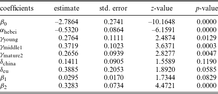
(5) \begin{equation} \begin{aligned} \ln \lambda^{\text{(GLM)}}(\textbf{x})=&\beta_0+\alpha_{\text{hebei}}+\gamma_{\text{young}}+\gamma_{\text{middle1}}+\gamma_{\text{mature2}}+\delta_{\text{china}}+\delta_{\text{eu}}\\[5pt]& + \beta_1\text{car_age}+\beta_2\text{trun_logged_distance}. \end{aligned}\end{equation}

Hence, we have merged Shanghai Province and other regions with Zhejiang Province, middle age 2 with mature age 1, and car made in Japan, Korea, and US with Germany. Also, we have removed gender from the full model (4). The estimated coefficients are listed in Table 3. Therefore, drivers in Hebei Province have a lower claims frequency than those in Zhejiang Province, and drivers aged 18 to 32 and older than 45 have a higher claims frequency than those aged 33 to 44. Claims frequencies are not significantly different among different car made countries. Furthermore, claims frequency is increasing log-linearly with both car’s age and average daily driving distance.

Table 3

The estimated coefficients in the GLM (5).

The out-of-sample Poisson deviance loss (3) for model (5) is $1.0306$ , compared with $1.1003$ for a homogeneous model

(6) \begin{equation} \ln\lambda^{\text{(Homo)}}(\textbf{x})=\beta_0.\end{equation}

Hence, with classical actuarial risk factors insurers can better understand risk heterogeneity of the portfolio and divide it into several homogeneous risk groups.

Remarks. We have also fitted a generalized boosted regression model and a XGBoost. It turns out that the out-of-sample Poisson deviance loss is not improved by those two boosting methods. Please refer to Sections 3.3.1 and 3.3.2 of Gao et al. (Reference Gao, Wang and Wüthrich2021) for more details. Thus, the GLM (5) has sufficiently captured the prediction power of those risk factors. It may be attributed to the appropriateness of our preprocessing of covariates and the nonexistence of significant interaction effects. On the other hand, our data only contain $n=1847$ cars with 4215 years exposure, so we may not discover potential nonlinear effects and interaction effects based on such a small portfolio. In addition, one may consider a zero-inflated Poisson (ZIP) model to address the excess of zero claims. This has been outlined in Section 6 as directions for future works.

4.1. Selection of archetypal drivers

Ideally, reasonable risk scores of individual trips should improve our claims frequency predictions. More specifically, reasonable risk scores should explain some variations in residuals of the GLM (5). This motivates how we select archetypal drivers and label their trips. We calculate the deviance residuals of the Poisson GLM (5) as follows:

\begin{align*}r_i =\, & \text{sign}\left(N_i-e_i\hat{\lambda}^{\text{(GLM)}}(\textbf{x}_i)\right)\\[5pt]& \times \sqrt{2e_i\hat{\lambda}^{\text{(GLM)}}(\textbf{x}_i)-2N_i-2N_i \ln \left(e_i\hat{\lambda}^{\text{(GLM)}}\right)+2N_i\ln N_i}.\end{align*}

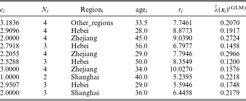
We select 10 drivers with the largest deviance residuals in the learning data $\mathcal{D}_{\text{learn}}$ as archetypal risky drivers and label their 5000 trips as potentially risky trips (coded as $R_{i,j}=1$ ). For those archetypal risky drivers, their exposure, number of claims, region, age, deviance residuals, and estimated claims frequency in GLM (5) are listed in Table 4. They have made at least 2 claims in total, but the average estimated claims frequency is only $20.06\%$ from GLM (5). We anticipate that those drivers may have a risky driving behavior not coded in age, region, or other classical risk factors.

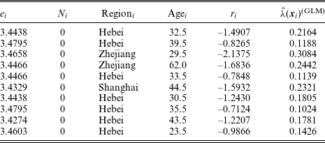
We then select 10 drivers with no claim and the largest exposure in the learning data $\mathcal{D}_{\text{learn}}$ as archetypal safe drivers and label their 5000 trips as potentially safe trips (coded as $R_{i,j}=0$ ). For those archetypal safe drivers, their exposure, number of claims, region, age, deviance residuals, and estimated claims frequency in GLM (5) are listed in Table 5. The average estimated claims frequency is $18.37\%$ . We denote the index set of the archetypal drivers by $\mathcal{I}_{\text{sel}}$ .

Table 4

10 archetypal risky drivers.

Table 5

10 archetypal safe drivers.

Remarks. We do not select drivers with the smallest residuals. The reason is that the corresponding drivers to this criterion will be those with high estimated claims frequency but no claims. Such drivers can be potentially risky drivers, since even the true claims frequency is high, the chance of making no claim is also high. Our attempts show that if we chose those drivers with the smallest residuals, we would not calibrate a useful 1D CNN for the goal of improving the GLM.

4.2. A one-dimensional convolutional neural network

We add two more telematics variables, squared acceleration rates $a^2$ and squared angle changes $\Delta^2$ , to time series of individual trips. Those second moments measure the variation in acceleration and angle change, which are related to one’s driving style. From the perspective of the universality approximation theorem (Hornik et al. Reference Hornik, Stinchcombe and White1989), although including those variables may not be necessary, doing so may improve the model fitting on relatively small samples. We normalize telematics variables $v, a, \Delta, a^2$ and $\Delta^2$ using the min-max normalization, that is, $z_{i,j}\in[-1,1]^{300\times 5}$ for $i\in\mathcal{I}_{\text{sel}}, j=1,\ldots, 500.$ Note that all archetypal drivers have 500 trips. We have labeled the trips of 10 archetypal risky drivers as $R_{i,j}=1$ and those of archetypal safe drivers as $R_{i,j}=0$ . We split all trips $(R_{i,j},z_{i,j})_{i\in\mathcal{I}_{\text{sel}},j=1:500}$ into training data $(R_{i,j},z_{i,j})_{i\in\mathcal{I}_{\text{sel}}},$ $j=1:300$ , validation data $(R_{i,j},z_{i,j})_{i\in\mathcal{I}_{\text{sel}},j=301:400}$ , and test data $(R_{i,j},z_{i,j})_{i\in\mathcal{I}_{\text{sel}}},$ $j=401:500$ .

With R interface to keras and tensorflow, we construct a 1D CNN to classify the trips of selected archetypal drivers:

(7) \begin{equation} \phi: [-1,1]^{300\times5}\rightarrow (0,1), z\mapsto\phi(z).\end{equation}

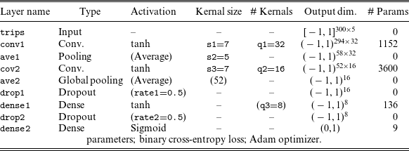
Using the keras code shown in Listing 1 of the supplementary material with q1=32, q2=16, q3=8, s1=7, s2=5, s3=7, rate1=0.5, rate2=0.5, we specify the feed-forward structure for a 1D CNN as shown in Table 6.

A 1D convolution layer cov1 extracts q1=32 features from a sliding window of s1=7 s. A average pooling layer ave1 calculates average of each feature for every s2=5 s without overlapping. Another 1D convolution layer cov2 further extracts q2=16 features from a sliding window of s3=7 s. A global average pooling layer ave2 calculates average of each feature along the entire time series. Two dropout layers drop1 and drop2 are inserted before two densely connected layers dense1 and dense2, respectively, to reduce overfitting. The first densely connected layer dense1 explores interactions among q2=16 features. The second densely connected (output) layer dense2 explores interactions among q3=8 features, which returns an output neuron in (0,1) via a sigmoid activation function, defined as risk score of trip z. If an output neuron $\phi(z)$ is closer to 1, then the corresponding trip z receives a higher risk score.

Table 6

The specification of 1D CNN.

The 1D CNN in Table 6 contains 4897 trainable parameters (network weights) $\theta$ . The loss function is selected as binary cross-entropy loss. The Adam optimizer is used to perform gradient decent, which leads to a local minimum of the binary cross-entropy loss w.r.t. network weights $\theta$ on training data $\textbf{T}_{\text{train}}=(R_{i,j},z_{i,j})_{i\in\mathcal{I}_{\text{sel}},j=1:300}$ :

\begin{align*}\mathcal{L}_{\text{CNN}}({\phi},\textbf{T}_{\text{train}}) = & -\frac{1}{300\times|\mathcal{I}_{\text{sel}}|}\sum_{i\in\mathcal{I}_{\text{sel}}}\sum_{j=1}^{300}R_{i,j}\log\phi(z_{i,j};\theta)\\[5pt]& +(1-R_{i,j})\log(1-\phi(z_{i,j};\theta)),\end{align*}

which is equivalent to the log-likelihood related to Bernoulli distribution.

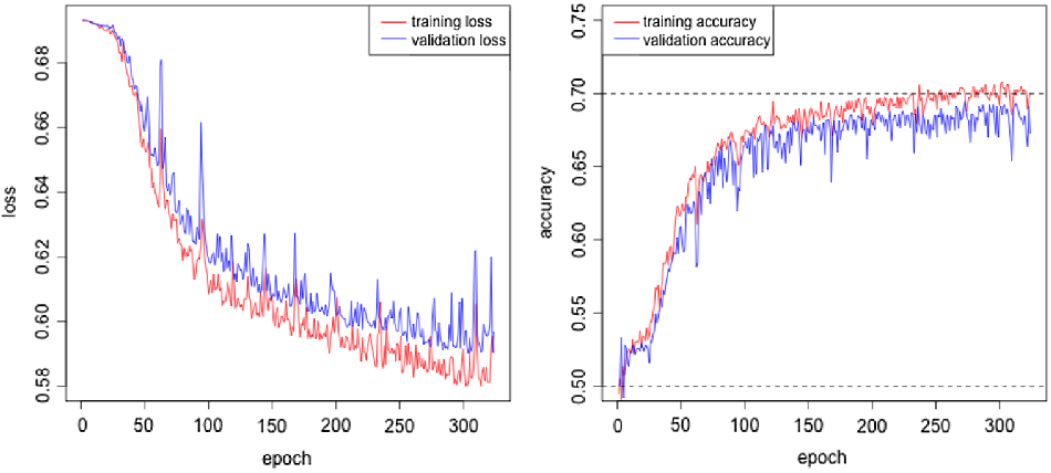
Using the keras code shown in Listing 2 of the supplementary material, we calibrate network weights $\theta$ for at most 1000 epoches. In each epoch, the gradient descent algorithm updates network weights for around $6000/512$ times. And in each update, 512 randomly selected training samples are used to calculate the gradient. This procedure is called stochastic gradient decent method, and the training loss on all training samples does not necessarily reduce after an epoch; see the non-monotonous trend in Figure 9. We stop calibration if the validation loss on $\textbf{T}_{\text{validation}}=(R_{i,j},z_{i,j})_{i\in\mathcal{I}_{\text{sel}},j=301:400}$ does not improve in a sequence of 20 consecutive epoches. The network weights $\hat{\theta}$ resulting in the lowest validation loss are then saved for the rest of modeling. The calibration shown in Figure 9 indicates that overfitting starts after 300 epoches, and the final validation accuracy is around 70%. Note that the hyperparameters of q1, q2, q3, s1, s2, s3 and dropout rates have been tuned by monitoring validation loss.

Figure 9:

Calibration of the 1D CNN in Table 6.

The calibrated 1D CNN $\hat{\phi}=\phi(\cdot;\hat{\theta})$ is employed to test trips $(R_{i,j}, z_{i,j})_{i\in\mathcal{I}_{\text{sel}},j=401:500}$ . The test accuracy is around 70%, which is much better than a random guess. We compare the distribution of test risk scores $\hat{\phi}(z_{i,j})$ for potentially risky trips with $R_{i,j}=1$ with that for potentially safe trips with $R_{i,k}=0$ in Figure 10. The test potentially risky trips tend to have higher risk scores than those of safe ones.

Figure 10:

Distributions of risk scores for test trips $(z_{i,j})_{i\in\mathcal{I}_{\text{sel}},j=401:500}$ .

Remarks. From our preliminary analyses, we found that the hyperbolic tangent activation is better than the relu activation function, and the average pooling is better than the max pooling for this particular classification task. Including squared acceleration rates and squared angle changes can improve prediction accuracy of 1D CNN. Moreover, one may choose the entire 500 trips of 6/2/2 archetypal risky drivers and 6/2/2 archetypal safe drivers as training/validation/test data, that is, splitting w.r.t. drivers rather than trips. However, according to our attempts, the neural network calibration is very sensitive to the partition, that is, the validation error cannot be reduced for some partitions. The reason may be that some archetypal safe drivers could still have many risky trips and vice versa.

4.3. Credibility average risk scores

The calibrated 1D CNN $\hat{\phi}$ is now employed to evaluate risk scores of $c_i$ individual trips for each driver i. We calculate average risk scores for each driver i:

(8) \begin{equation} \bar{\phi}_i=\frac{1}{c_i}\sum_{j=1}^{c_i}\hat{\phi}(z_{i,j}).\end{equation}

We consider robustness of average risk scores. Given a driver i, suppose that individual trips scores $\hat{\phi}(z_{i,j})$ identically and independently follow a distribution with expectation $\mu_i$ and standard deviation $\sigma_i$ . To fully credit an average risk score, it needs to be close to $\mu_i$ sufficiently with a high probability. In other words, the minimal number of trips is determined such that the following inequality holds:

(9) \begin{equation} \Pr(\mu_i-r\mu_i\le\bar{\phi}_i\le\mu_i+r\mu_i)\ge 1-\alpha.\end{equation}

This implies that average risk score has at least $(1-\alpha)$ chance lying in a short interval $[\mu_i-r\mu_i, \mu_i+r\mu_i]$ around $\mu_i$ . As detailed in the supplementary material, the minimal number of required trips is derived as

(10) \begin{equation} c^{(f)}_i(\alpha,r)=\left(\frac{\Phi^{-1}(1-\alpha/2)}{r}\right)^2\left(\frac{\sigma_i}{\mu_i}\right)^2,\end{equation}

where $\Phi^{-1}$ is the inverse of standard normal distribution function. Equation (10) is then employed as the standard of full credibility for an average risk score $\bar{\phi}_i$ . If the number of individual trips does not meet this standard, we can use the credibility average risk score instead

\begin{equation*}\tilde{\phi}_i=Z_i\bar{\phi}_i+(1-Z_i)\mu,\end{equation*}

where

\begin{equation*}Z_i=\min\left(1,\sqrt{\frac{c_i}{c_i^{(f)}}}\right),\end{equation*}

is partial credibility, and $\mu$ is the overall expectation of individual trip risk score. We select $\alpha=10\%, r=10\%$ and estimate parameters by the corresponding sample statistics:

(11) \begin{equation} \begin{aligned} \hat{\mu}_i&=\bar{\phi}_i\\[3pt] \hat{\sigma}_i&=\frac{1}{c_i-1}\sqrt{\sum_{j=1}^{c_i}\left(\hat{\phi}(z_{i,j})-\bar{\phi}_i\right)^2}\\[3pt] \hat{\mu}&=\frac{\sum_{i=1}^n c_i\bar{\phi}_i}{\sum_{i=1}^n c_i}. \end{aligned}\end{equation}

The histograms of partial credibilities and credibility average risk scores are displayed in Figure 11. Around 200 drivers meet the standard of full credibility for average risk score, and most drivers have partial credibility larger than $0.8$ . Thus, for most drivers, the credibility average risk scores are mainly determined by their own driving trips.

Figure 11:

Histograms of partial credibilities and credibility average risk scores.

5.1. Claims frequency modeling with credibility average risk scores

We improve the GLM (5) with credibility average risk score in another GLM as follows:

(12) \begin{equation} \ln \lambda(\textbf{x})= \ln \hat{\lambda}^{\text{(GLM)}}(\textbf{x})+ \ln {\lambda}^{\text{(TEL)}}(\textbf{x}),\end{equation}

where $\hat{\lambda}^{\text{(GLM)}}(\textbf{x})$ is the estimated claims frequency in GLM (5) and being treated as an offset term, and the (logged) telematics modification factor is

\begin{equation*}\ln {\lambda}^{\text{(TEL)}}(\textbf{x})= \beta_3+\beta_4\tilde{\phi}.\end{equation*}

Note that we have expanded the covariate space $\mathcal{X}$ to include the credibility average risk score. In actuarial practices, $\hat{\lambda}^{\text{(GLM)}}$ is corresponding to a pure premium charged at the inception of a policy, and ${\lambda}^{\text{(TEL)}}$ is a posterior telematics modification factor based on driving experience during the policy. Similar to design of bonus-malus system, premiums of policy renewals can be based on the telematics modification factor.

It turns out that the out-of-sample Poisson deviance loss for GLM (12) is $1.0286$ , improved over $1.0306$ for the GLM (5). The estimated telematics modification factor is

\begin{equation*}\hat{\lambda}^{\text{(TEL)}}=\exp(\hat{\beta}_3+\hat{\beta}_4\tilde{\phi})=\exp(-0.8859+1.7795\times\tilde{\phi}).\end{equation*}

Credibility average risk scores for all drivers are in $(0.1763,0.6810)$ , so the telematics modification factors fall in $(0.5643,1.3855)$ , which is quite reasonable. We plot the histogram of telematics modification factors for all drivers in Figure 12, which implies that most drivers have a telematics modification factor between $0.8$ and $1.2$ .

Figure 12:

Histogram of telematics modification factors for all drivers. Comparison of credibility average risk scores for all drivers obtained from 1D CNN and logistic regression.

Remarks. One may consider to calibrate a Poisson 1D CNN on all drivers’ trips with claims counts as response variable. However, such a calibration fails using either individual trips or jointed trips. One may consider to add credibility average risk score to GLM (5) and estimate all coefficients simultaneously, which actually leads to a similar result as that of GLM (12).

5.2. Competing methods

In this subsection, we first discuss one alternative to 1D CNN, then compare the proposed method with two alternative methods. All those alternative models need the input of manually engineered features of telematics variables.

5.2.2. Two alternative models to (12)

We consider two alternative models to (12), both of which use the manually engineered features $\textbf{s}_{i,j}$ as discussed in Section 5.2.1.

Alternative 1: Averaged telematics summary statistics. We calculate the average of summary statistics $\textbf{s}_{i,j}$ over all trips j for each driver i:

\begin{equation*}\textbf{u}_{i}=\frac{1}{c_i}\sum_{j=1}^{c_i}\textbf{s}_{i,j}.\end{equation*}

Those averaged telematics summary statistics $\textbf{u}_i\in{\mathbb R}^{35}$ are then used as covariates in the Poisson GLM for claims frequency prediction:

(13) \begin{equation} \ln \lambda(\textbf{x})= \ln \hat{\lambda}^{\text{(GLM)}}(\textbf{x})+ \ln {\lambda}^{\text{(ALT1)}}(\textbf{u}) =\ln \hat{\lambda}^{\text{(GLM)}}(\textbf{x})+ \langle\beta^{(u)},\textbf{u}\rangle,\end{equation}

where $\beta^{(u)}\in{\mathbb R}^{36}$ includes an intercept. We then conduct a step-wise variable selection based on the AIC. The test Poisson deviance loss is $1.0379$ which is even worse than that of the GLM (5) with classical actuarial risk factors.

Alternative 2: Risk scoring with a logistic regression. This alternative method follows the same procedure as our proposed method, but replaces the 1D CNN by a logistic regression as discussed in Section 5.2.1. We have the following alternative model:

(14) \begin{align} \ln \lambda(\textbf{x})=\ln \hat{\lambda}^{\text{(GLM)}}(\textbf{x})+ \ln {\lambda}^{\text{(ALT2)}}(\textbf{s})= \ln \hat{\lambda}^{\text{(GLM)}}(\textbf{x})+ \beta_3+\beta_4\tilde{\phi}^{\text{(ALT2)}}(\textbf{s}),\nonumber\\\end{align}

where $\tilde{\phi}^{\text{(ALT2)}}(\textbf{s})$ is the credibility average risk score by the logistic regression $\hat{\phi}^{\text{(ALT2)}}(\textbf{s})$ based on individual trips summary statistics $\textbf{s}$ . This alternative method also uses 35 manually engineered features $\textbf{s}_{i,j}$ , whereas our proposed method uses automatically engineered features by the neural network. The test Poisson deviance loss is $1.0287$ for this alternative model, which is close to that of our proposed method ( $1.0286$ ). Figure 12 compares credibility average risk scores for all drivers from the logistic regression and the 1D CNN with a correlation of $0.9153$ , which implies that both models return similar risk scores, that is, $\hat{\phi}^{\text{(ALT2)}}(\textbf{s}_{i,j})\approx\hat{\phi}(z_{i,j})$ .

5.3. Sensitivity analysis

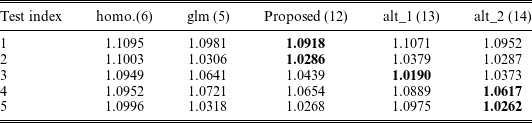
Since our portfolio size is relatively small, we conduct a sensitivity analysis to test the robustness of our results. Similar to cross-validation, we repeat the above analysis 5 times and evaluate test Poisson deviance loss on 5 mutually exclusive test data for the homogeneous model (6), the GLM with classical actuarial risk factors (5), our proposed model (12), and two alternative models (13) and (14), respectively. The results are shown in Table 7. Note that the above analysis corresponds to test index 2.

Table 7

Test Poisson deviance loss for different data partitions.

We conclude that the second alternative model (14) performs as well as our proposed method, and the first alternative model (13) is the least robust. Despite its simple specification and calibration, the second alternative model (14) relies on manually engineered features, which require thorough considerations. In contrast, our proposed method learns the representations automatically from time series of individual trips, and thus needs less manual intervention.