1 Introduction
Control of turbulent flow for drag reduction has the potential to yield significant economic and environmental benefits. Motivated by these potential benefits, many passive and active control techniques have been proposed in the previous literature. Techniques to reduce pressure drag (e.g. via shape optimization, active separation control) have been employed widely in practical applications. However, control schemes that reduce turbulent skin friction have seen much more limited implementation in real-world systems. As a result, the development of effective and practicable control schemes for skin friction reduction continues to be an important research problem.
It is commonly accepted that, for wall-bounded turbulent flows, the coherent structures associated with the energetic near-wall cycle play an important role in generating skin friction, at least at low-to-moderate Reynolds numbers. These near-wall coherent structures have been studied extensively since they were first observed in turbulent boundary layer experiments by Kline et al. (Reference Kline, Reynolds, Schraub and Rundstadler1967) and later reproduced in direct numerical simulation (DNS) by Kim, Moin, & Moser (Reference Kim, Moin and Moser1987). As reviewed by Robinson (Reference Robinson1991), the near-wall cycle comprises alternating high- and low-speed regions (‘streaks’) that are aligned in the streamwise direction and generated by the action of the quasi-streamwise vortices (QSVs). Further, it has been demonstrated that these coherent structures are maintained autonomously via a regeneration process that is independent of the outer region of the turbulent flow (Hamilton, Kim & Waleffe Reference Hamilton, Kim and Waleffe1995; Waleffe Reference Waleffe1997). Specifically, QSVs create streaks through interaction with the mean shear,
 $\text{d}U/\text{d}y$
. These streaks give rise to a spatially dependent velocity profile that is unstable, leading to a breakdown into streamwise-varying disturbances. A nonlinear mechanism involving these disturbances sustains the QSVs. Kim & Lim (Reference Kim and Lim2000) numerically investigated the relative effect of the nonlinear term and the linear interaction between the QSVs and the mean shear. This investigation showed that the linear interaction is essential for near-wall turbulence to be self-sustaining (i.e. turbulence decays if the mean shear is artificially set to zero), though the nonlinear term plays an important role in giving rise to the specific structures observed. Based on the studies outlined above, it has been hypothesized that effective interruption of this self-sustaining near-wall process could yield substantial turbulent skin friction reduction.
1.1 Feedback control for friction drag reduction
Many passive and active control methods have been proposed for turbulent skin friction reduction. Passive control techniques include the use of riblets, which are surface-mounted longitudinal microgrooves (Walsh Reference Walsh1983), and the addition of drag-reducing agents such as high-molecular-mass polymers or surfactants (e.g. White & Mungal Reference White and Mungal2008). Active control techniques can be further classified into predetermined (or open-loop) control and feedback flow control schemes. Representative examples of open-loop control that have been studied extensively include the use of spanwise wall oscillations (Jung, Mangiavacchi & Akhavan Reference Jung, Mangiavacchi and Akhavan1992), streamwise standing or travelling waves of spanwise wall forcing (Quadrio, Ricco & Viotti Reference Quadrio, Ricco and Viotti2009; Viotti, Quadrio & Luchini Reference Viotti, Quadrio and Luchini2009), as well as travelling waves of blowing and suction (Min et al. Reference Min, Kang, Speyer and Kim2006; Mamori, Iwamoto & Murata Reference Mamori, Iwamoto and Murata2014) or wall deformation (Hoepffner & Fukagata Reference Hœpffner and Fukagata2009; Nakanishi, Mamori & Fukagata Reference Nakanishi, Mamori and Fukagata2012).
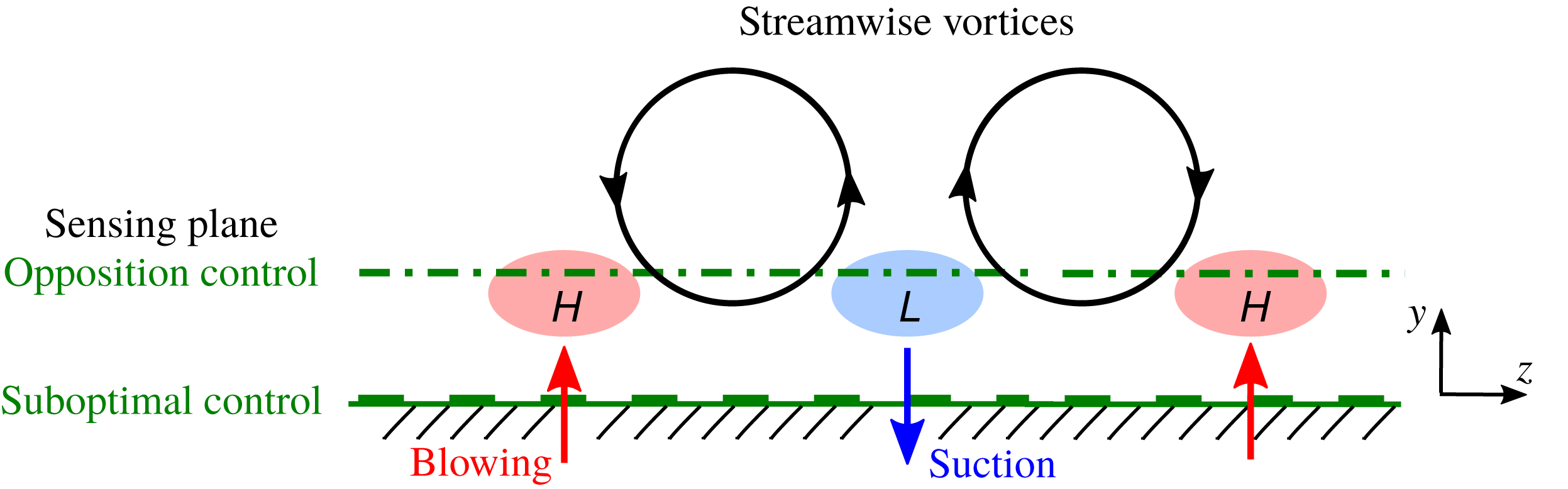
As for active feedback control, one widely studied scheme is opposition control, proposed by Choi, Moin & Kim (Reference Choi, Moin and Kim1994). As shown in figure 1, this technique aims to suppress QSVs by applying blowing and suction at the wall that opposes the wall-normal velocity detected by a sensor at some specified distance above the wall. This creates a virtual wall that hinders the wall-normal transport of streamwise momentum and interrupts the formation of streaks. In their DNS of channel flow at friction Reynolds number
 $Re_{\unicode[STIX]{x1D70F}}=u_{\unicode[STIX]{x1D70F}}\unicode[STIX]{x1D6FF}/\unicode[STIX]{x1D708}=180$
(for uncontrolled flow), Choi et al. (Reference Choi, Moin and Kim1994) demonstrated that
 $25\,\%$
drag reduction can be attained when the detection plane is set at
 $y^{+}\approx 10$
. Following standard notation,
 $u_{\unicode[STIX]{x1D70F}}$
is the friction velocity,
 $\unicode[STIX]{x1D6FF}$
is the channel half-width,
 $\unicode[STIX]{x1D708}$
is the kinematic viscosity, and a superscript
 $^{+}$
denotes normalization with respect to
 $u_{\unicode[STIX]{x1D70F}}$
and
 $\unicode[STIX]{x1D708}$
. The effects of opposition control have been examined further in many subsequent studies: Iwamoto, Suzuki & Kasagi (Reference Iwamoto, Suzuki and Kasagi2002) showed that control performance degrades with increasing Reynolds number; Chung & Talha (Reference Chung and Talha2011) evaluated the combined effect of sensor location and actuation amplitude (i.e. magnitude of blowing and suction) on control performance; Deng et al. (Reference Deng, Xu, Huang and Cui2014) further tested the effect of actuation amplitude; Lee (Reference Lee2015) studied control performance with discrete sensing; and more recently, Deng, Huang & Xu (Reference Deng, Huang and Xu2016) re-examined control performance degradation by pursuing DNS at higher friction Reynolds number,
 $Re_{\unicode[STIX]{x1D70F}}=1000$
.
Although conceptually simple, opposition control is impracticable because it requires velocity information above the wall. To overcome this issue, Lee, Kim & Choi (Reference Lee, Kim and Choi1998) proposed suboptimal control which only relies on information measurable at the wall (figure 1). Specifically, the control laws derived theoretically by Lee et al. (Reference Lee, Kim and Choi1998) require either the wall pressure, the spanwise wall shear stress, or the streamwise wall shear stress. Based on assessment in DNS, Lee et al. (Reference Lee, Kim and Choi1998) reported a 16–22 % reduction in skin friction when information about the wall pressure or the spanwise wall shear stress was used for the feedback control scheme, and a small drag increase when the streamwise wall shear stress information was used for control. These results are unfortunate since, for practical implementation, measurements of streamwise wall shear stress are often more reliable and easier to obtain. Following Lee et al. (Reference Lee, Kim and Choi1998), Choi & Sung (Reference Choi and Sung2002) investigated the influence of actuation amplitude and time scale on suboptimal control performance. Fukagata & Kasagi (Reference Fukagata and Kasagi2004) modified the proposed suboptimal control laws by considering a cost function related to the Reynolds shear stress. These modified laws led to drag reduction in turbulent pipe flow using only streamwise wall shear stress information.
The effectiveness of feedback control schemes has been evaluated to a certain extent via wind-tunnel experiments using arrays of miniature wall shear stress sensors and actuators (e.g. Rebbeck & Choi Reference Rebbeck and Choi2001, Reference Rebbeck and Choi2006; Yoshino, Suzuki & Kasagi Reference Yoshino, Suzuki and Kasagi2008; Kasagi, Suzuki, & Fukagata Reference Kasagi, Suzuki and Fukagata2009). However, most previous studies in this realm have relied on DNS. Accurate DNS can be expensive computationally, particularly as Reynolds number increases. For instance, Kolmogorov scaling suggests that the number of grid points must increase as Reynolds number to the power of
 $9/4$
(e.g. Kajishima & Taira Reference Kajishima and Taira2017). As a result, DNS remains prohibitively expensive for parametric studies at high Reynolds number, e.g. for trial-and-error evaluation of new control schemes. Therefore, there is significant scope for model-based design of feedback flow control for turbulent skin friction reduction.
Schematic of opposition control and suboptimal control.

1.2 Resolvent analysis
Models based on resolvent analysis (McKeon & Sharma Reference McKeon and Sharma2010) have demonstrated an ability to generate predictions consistent with structural and statistical features of wall-bounded turbulent flows (e.g. Moarref et al. Reference Moarref, Sharma, Tropp and McKeon2013; Sharma & McKeon Reference Sharma and McKeon2013). In addition, as illustrated by Luhar, Sharma & McKeon (Reference Luhar, Sharma and McKeon2014) and Nakashima, Fukagata & Luhar (Reference Nakashima, Fukagata and Luhar2017), resolvent analysis also has the potential to serve as a powerful tool that can predict the effects of active feedback control at low computational cost.
The resolvent formulation interprets the Fourier-transformed Navier–Stokes equations as a forcing–response system with nonlinear feedback. The turbulent velocity is considered as an output generated via the action of a linear transfer function (the resolvent operator) on the nonlinear terms. In other words, for every wavenumber–frequency combination, the linear resolvent operator maps the nonlinear forcing to the velocity field. A singular-value decomposition (SVD) of the discretized resolvent operator predicts regions of high energy amplification across spectral space (i.e. wavenumber–frequency combinations with high singular values) and identifies the form, or structure, of the velocity fields that are most amplified at each wavenumber–frequency combination. The high-gain velocity structures identified through this procedure are termed ‘resolvent modes’.
High-gain resolvent modes at specific wavenumber–frequency combinations have been shown to serve as useful surrogates for dynamically important flow features (McKeon & Sharma Reference McKeon and Sharma2010; Sharma & McKeon Reference Sharma and McKeon2013). As a result, this analysis enables an evaluation of control on coherent structures such as the near-wall (NW) cycle discussed above, as well as the very-large-scale motions (VLSMs) or superstructures that have been observed at high Reynolds numbers. Previous studies have employed resolvent analysis to evaluate the effects of opposition control (Luhar et al. Reference Luhar, Sharma and McKeon2014) and compliant walls (Luhar, Sharma & McKeon Reference Luhar, Sharma and Mckeon2015, Reference Luhar, Sharma and Mckeon2016), showing that relatively simple models are able to reproduce trends observed in DNS and large-eddy simulation (LES) with minimal computation. For a more comprehensive discussion of the resolvent formulation and related modelling efforts, the reader is referred to McKeon (Reference McKeon2017).
Recently, Nakashima et al. (Reference Nakashima, Fukagata and Luhar2017) pursued resolvent analysis to elucidate the physical mechanisms leading to drag reduction for the suboptimal control method proposed by Lee et al. (Reference Lee, Kim and Choi1998). In addition to examining the effects of control on individual resolvent modes resembling the NW cycle and VLSMs, Nakashima et al. (Reference Nakashima, Fukagata and Luhar2017) also considered the effects of control across spectral space. Resolvent-based predictions suggested that suboptimal control performance is mixed across spectral space when the fluctuating streamwise wall shear stress is used as the control input. In particular, it was shown that suboptimal control suppresses spatio-temporal modes with long streamwise wavelengths (i.e. singular values are reduced) but further amplifies modes with shorter streamwise wavelengths. Based on this observation, it was hypothesized that control performance may be improved if control is applied selectively over the spectral region in which singular values decrease, or if a new control law is designed such that resolvent modes are suppressed across all of spectral space.
Although resolvent analysis provides this valuable insight into the effect of control on linear amplification mechanisms, it is unable to predict the effect of control on nonlinear interaction between individual wavenumber–frequency combinations. Therefore, the effects of any control laws proposed using resolvent analysis must ultimately be assessed via DNS or experiments.
1.3 Outline
A central objective of the present study is to assess the performance of suboptimal control for selective wavelengths by means of DNS. In addition, we propose new control laws that require only streamwise wall shear stress information using resolvent analysis, and evaluate their effects via DNS. The remainder of this paper is organized as follows. The theory behind suboptimal control and the numerical methods are described in § 2. DNS results for suboptimal control for selective wavelengths are shown in § 3.1. Resolvent analysis is used to develop new control laws in § 3.2. Evaluation of these new control laws via DNS is carried out in § 3.3. A dynamical interpretation of the newly developed control laws, based on conditional sampling of the controlled velocity fields, is provided in §§ 4.1 and 4.2. Conclusions are presented in § 5.
2 Theory and numerical methods
The base case being considered is an incompressible, fully developed turbulent channel flow, for which the governing Navier–Stokes equations and continuity constraint can be expressed as
 $$\begin{eqnarray}\displaystyle & \displaystyle \frac{\unicode[STIX]{x2202}u_{i}}{\unicode[STIX]{x2202}x_{i}}=0, & \displaystyle\end{eqnarray}$$
 $$\begin{eqnarray}\displaystyle & \displaystyle \frac{\unicode[STIX]{x2202}u_{i}}{\unicode[STIX]{x2202}t}=-\frac{\unicode[STIX]{x2202}u_{j}u_{i}}{\unicode[STIX]{x2202}x_{j}}-\frac{\unicode[STIX]{x2202}p}{\unicode[STIX]{x2202}x_{i}}+\frac{1}{Re_{\unicode[STIX]{x1D70F}}}\frac{\unicode[STIX]{x2202}^{2}u_{i}}{\unicode[STIX]{x2202}x_{j}\unicode[STIX]{x2202}x_{j}}. & \displaystyle\end{eqnarray}$$
Here
 $x_{1}$
,
 $x_{2}$
and
 $x_{3}$
denote the streamwise, wall-normal and spanwise directions, respectively,
 $u_{i}$
are the corresponding velocity components,
 $t$
is the time and
 $p$
is the pressure. All variables are made dimensionless using the density
 $\unicode[STIX]{x1D70C}$
, the friction velocity
 $u_{\unicode[STIX]{x1D70F}}$
, and the channel half-width
 $\unicode[STIX]{x1D6FF}$
. As before, the friction Reynolds number is
 $Re_{\unicode[STIX]{x1D70F}}=u_{\unicode[STIX]{x1D70F}}\unicode[STIX]{x1D6FF}/\unicode[STIX]{x1D708}$
, in which
 $\unicode[STIX]{x1D708}$
denotes the kinematic viscosity. Hereafter, a superscript
 $^{+}$
denotes inner normalization based on
 $u_{\unicode[STIX]{x1D70F}}$
for the uncontrolled flow and
 $\unicode[STIX]{x1D708}$
. For the uncontrolled case, the no-slip boundary condition applies. For suboptimal control, the boundary conditions are modified to account for the effect of blowing and suction, i.e. there is a non-zero wall-normal velocity at the wall.
2.1 Suboptimal control
Based on observations that opposition control (Choi et al. Reference Choi, Moin and Kim1994) induces spanwise flow below QSVs from high-pressure regions to low-pressure regions, marked as H and L, respectively, in figure 1, Lee et al. (Reference Lee, Kim and Choi1998) considered the following cost function, which aims to increase spanwise wall shear stress:
 $$\begin{eqnarray}\displaystyle J(\unicode[STIX]{x1D719})=\frac{l}{2A\unicode[STIX]{x0394}t}\int _{S}\int _{t}^{t+\unicode[STIX]{x0394}t}\unicode[STIX]{x1D719}^{2}\,\text{d}t\,\text{d}S-\frac{1}{2A\unicode[STIX]{x0394}t}\int _{S}\int _{t}^{t+\unicode[STIX]{x0394}t}\left(\frac{\unicode[STIX]{x2202}w}{\unicode[STIX]{x2202}y}\right)_{w}^{2}\,\text{d}t\,\text{d}S. & & \displaystyle\end{eqnarray}$$
In the expression above,
 $\unicode[STIX]{x1D719}$
represents the wall-normal velocity at the wall (i.e. the control input),
 $A$
is the area of the wall, and
 $l$
is the relative energetic cost of control. Based on a minimization of (2.3), the suboptimal control law was derived in Fourier space as
 $$\begin{eqnarray}\displaystyle \text{(case SP)}:\qquad \hat{\unicode[STIX]{x1D719}}=\unicode[STIX]{x1D6FC}\frac{\text{i}k_{z}}{K}\left(\widehat{\frac{\unicode[STIX]{x2202}w}{\unicode[STIX]{x2202}y}}\right)_{w}. & & \displaystyle\end{eqnarray}$$
Here, the hat
 $\hat{(\cdot )}$
denotes a specific Fourier component,
 $\unicode[STIX]{x1D6FC}$
is a scalar coefficient representing blowing-and-suction magnitude, and
 $K=\sqrt{k_{x}^{2}+k_{z}^{2}}$
in which
 $k_{x}$
and
 $k_{z}$
are the streamwise wavenumber and spanwise wavenumber, respectively. Hereafter, the control law expressed in (2.4), which requires measurements of the spanwise wall shear stress, is termed case SP. Lee et al. (Reference Lee, Kim and Choi1998) attained a 22 % drag reduction using this law in their channel flow DNS at
 $Re_{\unicode[STIX]{x1D70F}}=110$
.
Lee et al. (Reference Lee, Kim and Choi1998) also proposed another control law, for which the cost function was defined as
 $$\begin{eqnarray}\displaystyle J(\unicode[STIX]{x1D719})=\frac{l}{2A\unicode[STIX]{x0394}t}\int _{S}\int _{t}^{t+\unicode[STIX]{x0394}t}\unicode[STIX]{x1D719}^{2}\,\text{d}t\,\text{d}S+\frac{1}{2A\unicode[STIX]{x0394}t}\int _{S}\int _{t}^{t+\unicode[STIX]{x0394}t}\left(\frac{\unicode[STIX]{x2202}u}{\unicode[STIX]{x2202}y}\right)_{w}^{2}\,\text{d}t\,\text{d}S. & & \displaystyle\end{eqnarray}$$
This cost function was designed to generate a reduction in the streamwise wall shear stress, which is directly related to turbulent skin friction. A minimization of (2.5) led to the following control law:
 $$\begin{eqnarray}\displaystyle \text{(case ST)}:\qquad \hat{\unicode[STIX]{x1D719}}=-\unicode[STIX]{x1D6FC}\frac{\text{i}k_{x}}{K}\left(\widehat{\frac{\unicode[STIX]{x2202}u}{\unicode[STIX]{x2202}y}}\right)_{w}. & & \displaystyle\end{eqnarray}$$
This law, which relies on measurement of the streamwise wall shear stress, is referred to as case ST. DNS results presented in Lee et al. (Reference Lee, Kim and Choi1998), however, indicated that this control law leads to an increase in drag.
In this study, we first assess the effect of the control laws described by (2.4) and (2.6) for limited regions in spectral space, identified based on predictions from resolvent analysis. Numerically, control is implemented via the following procedure. First, based on (2.4) and (2.6), we determine the control input for all (
 $k_{x},k_{z}$
) combinations. Then, the input is introduced only for the wavenumber combinations corresponding to the spectral region of interest; for the remaining wavenumber combinations, the inputs are set at zero. In the numerical simulations described below, the amplitude parameter
 $\unicode[STIX]{x1D6FC}$
is set such that the root-mean-square (r.m.s.) value of the blowing-and-suction velocity,
 $\unicode[STIX]{x1D719}$
, equals the r.m.s. value of the wall-normal velocity at
 $y^{+}\approx 10$
for the uncontrolled case, similar to Lee et al. (Reference Lee, Kim and Choi1998).
2.2 Direct numerical simulations
We use the DNS code originally developed by Fukagata, Kasagi & Koumoutsakos (Reference Fukagata, Kasagi and Koumoutsakos2006). A second-order-accurate finite difference scheme is used for spatial discretization of (2.1) and (2.2), and time integration is carried out using a third-order-accurate Runge–Kutta/Crank–Nicolson scheme. The friction Reynolds number of the uncontrolled flow is set at
 $Re_{\unicode[STIX]{x1D70F}}=180$
. All the controlled simulations are conducted under a constant flow rate condition. The bulk mean velocity
 $U_{b}$
is maintained constant at the value obtained in the uncontrolled case. The drag reduction rate is defined as
 $$\begin{eqnarray}\displaystyle R_{D}=1-\frac{\overline{(-\text{d}p/\text{d}x)_{c}}}{\,\overline{(-\text{d}p/\text{d}x)_{0}}\,}, & & \displaystyle\end{eqnarray}$$
where subscripts
 $0$
and
 $c$
represent the uncontrolled case and controlled case, respectively.
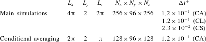
Computational conditions (domain size, grid resolution and time step) for each case are summarized in table 1. To ensure numerical stability, a different time step was employed depending on whether control was applied across all wavelengths (CA), or selectively for large scales (CL) or small scales (CS). The threshold wavelength used to distinguish between small and large scales was
 $\unicode[STIX]{x1D706}_{x}^{+}\approx 140$
. This threshold was identified via resolvent analysis, and is discussed further in § 3.1 below.
Table 1 also shows the domain size and number of grid points used for the conditional averaging discussed in § 4.1. The streamwise and spanwise extents of the computational domain were halved for this purpose, but the grid resolution was maintained constant. For verification, additional simulations with higher spatio-temporal resolution were also carried out. The number of grid points was increased to
 $N_{x}\times N_{y}\times N_{z}=512\times 96\times 256$
and
 $256\times 96\times 512$
, while
 $\unicode[STIX]{x0394}t$
was halved relative to the values shown in table 1. These additional simulations yielded very similar results. The differences in
 $R_{D}$
were found to be less than
 $1\,\%$
with the increased resolution.
Computational conditions for the DNS.

2.3 Resolvent analysis
To evaluate and design control laws, we employ an extension of the resolvent analysis formalism proposed by McKeon & Sharma (Reference McKeon and Sharma2010). The formulation is outlined briefly below. The numerical implementation employed here is identical to that described in Nakashima et al. (Reference Nakashima, Fukagata and Luhar2017).
Given the spatial homogeneity and statistical stationarity expected in turbulent channel flow, the analysis begins with a Fourier transform of the velocity and pressure fields in the streamwise and spanwise directions, and in time,
 $$\begin{eqnarray}\displaystyle \left[\begin{array}{@{}c@{}}\boldsymbol{u}(x,y,z,t)\\ p(x,y,z,t)\end{array}\right]=\iiint _{-\infty }^{\infty }\left[\begin{array}{@{}c@{}}\boldsymbol{u}_{\boldsymbol{k}}(y)\\ p_{\boldsymbol{k}}(y)\end{array}\right]\text{e}^{\text{i}(k_{x}x+k_{z}z-\unicode[STIX]{x1D714}t)}\,\text{d}k_{x}\,\text{d}k_{z}\,\text{d}\unicode[STIX]{x1D714}, & & \displaystyle\end{eqnarray}$$
in which
 $\unicode[STIX]{x1D714}$
represents temporal (angular) frequency. Each wavenumber–frequency combination
 $\boldsymbol{k}=(k_{x},k_{z},\unicode[STIX]{x1D714})$
represents a travelling-wave flow structure with streamwise wavelength
 $\unicode[STIX]{x1D706}_{x}=2\unicode[STIX]{x03C0}/k_{x}$
, spanwise wavelength
 $\unicode[STIX]{x1D706}_{z}=2\unicode[STIX]{x03C0}/k_{z}$
, and propagation speed
 $c=\unicode[STIX]{x1D714}/k_{x}$
. Note that these travelling waves are oblique in nature, with the spanwise propagation direction depending on the sign of
 $k_{z}$
relative to
 $k_{x}$
.
For a given wavenumber–frequency combination, the wall-normal variation in the velocity and pressure fields is identified via a gain-based decomposition of the Navier–Stokes equations. Under the Fourier transform, the governing equations, (2.1) and (2.2), can be expressed as
 $$\begin{eqnarray}\unicode[STIX]{x1D735}_{\boldsymbol{k}}\boldsymbol{\cdot }\boldsymbol{u}_{\boldsymbol{k}}=0\end{eqnarray}$$
and
 $$\begin{eqnarray}(-\text{i}\unicode[STIX]{x1D714}+\text{i}k_{x}U)\boldsymbol{u}_{\boldsymbol{k}}+\frac{\unicode[STIX]{x2202}U}{\unicode[STIX]{x2202}y}v_{\boldsymbol{k}}\boldsymbol{e}_{\boldsymbol{x}}+\unicode[STIX]{x1D735}p_{\boldsymbol{k}}-\frac{1}{Re_{\unicode[STIX]{x1D70F}}}\unicode[STIX]{x1D6FB}_{\boldsymbol{k}}^{2}\boldsymbol{u}_{\boldsymbol{ k}}=\boldsymbol{f}_{\boldsymbol{k}},\end{eqnarray}$$
where
 $\unicode[STIX]{x1D735}_{\boldsymbol{k}}=[\text{i}k_{x}~\unicode[STIX]{x2202}/\unicode[STIX]{x2202}y~\text{i}k_{z}]^{\text{T}}$
and
 $\unicode[STIX]{x1D735}_{\boldsymbol{k}}^{\text{T}}$
denote the gradient and divergence operators, respectively, and
 $\boldsymbol{f}_{\boldsymbol{k}}=(-\boldsymbol{u}\boldsymbol{\cdot }\unicode[STIX]{x1D735}\boldsymbol{u})_{\boldsymbol{k}}$
represents the Fourier-transformed nonlinear term. These equations are rearranged as follows:
 $$\begin{eqnarray}\displaystyle \left[\begin{array}{@{}c@{}}\boldsymbol{u}_{\boldsymbol{k}}\\ p_{\boldsymbol{k}}\end{array}\right] & = & \displaystyle \left(-\text{i}\unicode[STIX]{x1D714}\left[\begin{array}{@{}cc@{}}\unicode[STIX]{x1D644} & \\ & 0\end{array}\right]-\left[\begin{array}{@{}cc@{}}\boldsymbol{L}_{\boldsymbol{k}} & -\unicode[STIX]{x1D735}_{\boldsymbol{k}}\\ \unicode[STIX]{x1D735}_{\boldsymbol{k}}^{\text{T}} & 0\end{array}\right]\right)^{-1}\left[\begin{array}{@{}c@{}}\unicode[STIX]{x1D644}\\ 0\end{array}\right]\boldsymbol{f}_{\boldsymbol{k}}\end{eqnarray}$$
 $$\begin{eqnarray}\displaystyle & = & \displaystyle \boldsymbol{H}_{\boldsymbol{k}}\,\boldsymbol{f}_{\boldsymbol{k}},\end{eqnarray}$$
where the linear operator
 $\boldsymbol{L}_{\boldsymbol{k}}$
is defined as
 $$\begin{eqnarray}\displaystyle \boldsymbol{L}_{\boldsymbol{k}}=\left[\begin{array}{@{}ccc@{}}-\text{i}k_{x}U+Re_{\unicode[STIX]{x1D70F}}^{-1}\unicode[STIX]{x1D6FB}_{\boldsymbol{k}}^{2} & -(\unicode[STIX]{x2202}U/\unicode[STIX]{x2202}y) & 0\\ 0 & -\text{i}k_{x}U+Re_{\unicode[STIX]{x1D70F}}^{-1}\unicode[STIX]{x1D6FB}_{\boldsymbol{k}}^{2} & 0\\ 0 & 0 & -\text{i}k_{x}U+Re_{\unicode[STIX]{x1D70F}}^{-1}\unicode[STIX]{x1D6FB}_{\boldsymbol{k}}^{2}\end{array}\right] & & \displaystyle\end{eqnarray}$$
and
 $$\begin{eqnarray}\unicode[STIX]{x1D6FB}_{\boldsymbol{k}}^{2}=-k_{x}^{2}-(\unicode[STIX]{x2202}^{2}/\unicode[STIX]{x2202}y^{2})-k_{z}^{2}\end{eqnarray}$$
represents the Fourier-transformed Laplacian operator.
In essence, with the formulation shown above, the velocity and pressure fields
 $[\boldsymbol{u}_{\boldsymbol{k}}~p_{\boldsymbol{k}}]^{\text{T}}$
are expressed as a response of the linearized Navier–Stokes system to the nonlinear forcing term
 $\boldsymbol{f}_{\boldsymbol{k}}$
. For every wavenumber–frequency combination, the linear resolvent operator
 $\boldsymbol{H}_{\boldsymbol{k}}$
maps this nonlinear forcing to the velocity field. The analysis proceeds with an SVD of
 $\boldsymbol{H}_{\boldsymbol{k}}$
,
 $$\begin{eqnarray}\boldsymbol{H}_{\boldsymbol{k}}=\mathop{\sum }_{m}\boldsymbol{u}_{\boldsymbol{k},m}\unicode[STIX]{x1D70E}_{\boldsymbol{k},m}\,{\boldsymbol{f}_{\boldsymbol{k},m}}^{\ast },\end{eqnarray}$$
which yields a set of orthonormal forcing modes,
 $\boldsymbol{f}_{\boldsymbol{k},m}$
, and response modes,
 $\boldsymbol{u}_{\boldsymbol{k},m}$
, that are ordered based on the forcing–response gain,
 $\unicode[STIX]{x1D70E}_{\boldsymbol{k},m}$
, under an
 $L^{2}$
energy norm. The superscript
 $^{\ast }$
denotes the complex conjugate. Previous studies have shown that the resolvent operator is low-rank at wavenumber–frequency combinations that are energetic in wall-bounded turbulent flows. In other words, the lead singular value is much larger than subsequent singular values. As a result, reasonable models for flow statistics, structure and control can be generated under a rank-one approximation (McKeon & Sharma Reference McKeon and Sharma2010; Moarref et al.
Reference Moarref, Sharma, Tropp and McKeon2013; Sharma & McKeon Reference Sharma and McKeon2013; Luhar et al.
Reference Luhar, Sharma and McKeon2014), i.e. by considering the gain (
 $\unicode[STIX]{x1D70E}_{\boldsymbol{k},1}$
) and structure (
 $\boldsymbol{u}_{\boldsymbol{k},1}$
) of just the first singular modes across spectral space. Based on these prior observations and following Nakashima et al. (Reference Nakashima, Fukagata and Luhar2017), we also employ a rank-one approximation to analyse the effect of suboptimal control. Hereafter, the additional subscript
 $1$
is dropped, with the understanding that
 $\unicode[STIX]{x1D70E}_{\boldsymbol{k}}=\unicode[STIX]{x1D70E}_{\boldsymbol{k},1}$
.
The effect of suboptimal control is introduced in the analysis procedure described above by changing the boundary conditions to (2.4) or (2.6) prior to computing the resolvent operator. This change in boundary conditions relative to the uncontrolled case alters the gain and structure of the rank-one resolvent modes obtained under the SVD. We evaluate the efficacy of control by considering the squared ratio of controlled to uncontrolled (NC) singular value,
 $(\unicode[STIX]{x1D70E}_{\boldsymbol{k}c}/\unicode[STIX]{x1D70E}_{\boldsymbol{k}0})^{2}$
. If the ratio is less than unity (i.e.
 $1-(\unicode[STIX]{x1D70E}_{\boldsymbol{k}c}/\unicode[STIX]{x1D70E}_{\boldsymbol{k}0})^{2}>0$
), we assume the mode is suppressed under control, which results in lower drag. If the ratio is greater than unity, we assume the mode is further amplified, which contributes to an increase in drag.
Note that this singular-value-based assessment of control essentially assumes unit forcing at each wavenumber–frequency combination, such that the energy associated with each mode is simply
 $\unicode[STIX]{x1D70E}_{\boldsymbol{k}}^{2}$
(Luhar et al.
Reference Luhar, Sharma and McKeon2014). In other words, this analysis only considers the effect of control on the linear forcing–response amplification mechanism for each mode. Of course, control can also modify nonlinear interactions between different modes, which could alter the distribution of the forcing across spectral space. These nonlinear effects are neglected in the procedure described above, and so evaluation of control for the full nonlinear system via DNS is an essential component of the present study. Of course, there could be other ways to assess the control effect. For instance, prior resolvent-based analysis (Luhar et al.
Reference Luhar, Sharma and McKeon2014, Reference Luhar, Sharma and Mckeon2015; Nakashima et al.
Reference Nakashima, Fukagata and Luhar2017) adopted an indicator based on the Reynolds shear stress contribution (Fukagata, Iwamoto & Kasagi Reference Fukagata, Iwamoto and Kasagi2002), i.e.
 $R_{\boldsymbol{k}}=\int _{-1}^{1}\unicode[STIX]{x1D70E}_{\boldsymbol{k}}^{2}Re(u_{\boldsymbol{k}}^{\ast }v_{\boldsymbol{k}})(+y)\,\text{d}y$
, and Nakashima, Luhar & Fukagata (Reference Nakashima, Luhar and Fukagata2019) simply used
 $\unicode[STIX]{x1D70E}_{\boldsymbol{k}c}/\unicode[STIX]{x1D70E}_{\boldsymbol{k}0}$
. However, Nakashima et al. (Reference Nakashima, Fukagata and Luhar2017) show that the indicator based on the singular-value ratio and
 $R_{\boldsymbol{k}}$
give essentially similar results.
It is also worth noting that the coefficient
 $\unicode[STIX]{x1D6FC}$
in (2.4) and (2.6) is implemented in different ways in DNS and resolvent analysis. As discussed in § 2.1, in the DNS
 $\unicode[STIX]{x1D6FC}$
is set to ensure that
 $\unicode[STIX]{x1D719}_{rms}$
equals
 $v_{rms}$
for the uncontrolled case at
 $y^{+}\approx 10$
, i.e.
 $\unicode[STIX]{x1D719}_{rms}^{+}=v_{rms,0}^{+}(y^{+}\approx 10)=0.25$
. In contrast, in resolvent analysis
 $\unicode[STIX]{x1D6FC}$
is considered a design parameter and must be determined a priori. Of course, for a fair comparison between DNS and resolvent-based predictions, the value of
 $\unicode[STIX]{x1D6FC}$
must be maintained constant between the two cases.
3 Results
3.1 Case SP and case ST
First, we determine whether performance for suboptimal control can be maintained, or improved, via the use of a spatial wavenumber filter. In other words, we evaluate performance with control applied only over the spectral region where resolvent analysis predicts favourable effects. To generate resolvent-based predictions, we first need to identify appropriate values for the blowing-and-suction parameter
 $\unicode[STIX]{x1D6FC}$
.
Nakashima et al. (Reference Nakashima, Fukagata and Luhar2017) estimated the value of
 $\unicode[STIX]{x1D6FC}$
using two different approaches for case SP, although both methods assumed the NW cycle to be the dominant flow feature. First, based on known r.m.s. values of the fluctuating spanwise wall shear stress and the magnitude of blowing and suction obtained in previous DNS, this parameter was estimated from (2.4) in inner normalized form as
 $$\begin{eqnarray}\unicode[STIX]{x1D6FC}^{+}\approx \frac{K}{k_{z}}\frac{\unicode[STIX]{x1D719}_{rms}^{+}}{(\unicode[STIX]{x2202}w_{rms}/\unicode[STIX]{x2202}y)_{w}^{+}}\approx \frac{\unicode[STIX]{x1D719}_{rms}^{+}}{(\unicode[STIX]{x2202}w_{rms}/\unicode[STIX]{x2202}y)_{w}^{+}}.\end{eqnarray}$$
The expression above assumes that
 $K=\sqrt{k_{x}^{2}+k_{z}^{2}}\approx k_{z}$
, which is reasonable since the NW cycle comprises structures that are approximately one order of magnitude longer in the streamwise direction compared to the spanwise direction. Second, Nakashima et al. (Reference Nakashima, Fukagata and Luhar2017) estimated
 $\unicode[STIX]{x1D6FC}^{+}$
by requiring that
 $\unicode[STIX]{x1D719}_{\boldsymbol{k}}$
be approximately equal to
 $v_{\boldsymbol{k}}(y^{+}\approx 10)$
for resolvent modes resembling the NW cycle. More specifically, they considered the wavenumber–frequency combination corresponding to
 $(\unicode[STIX]{x1D706}_{x}^{+},\unicode[STIX]{x1D706}_{z}^{+},c^{+})\approx (10^{3},10^{2},10)$
as being representative of the NW cycle since the energetic contribution associated with these structures is known to be concentrated around
 $(\unicode[STIX]{x1D706}_{x}^{+},\unicode[STIX]{x1D706}_{z}^{+})\approx (10^{3},10^{2})$
in spectral space and near the wall-normal location
 $y^{+}\approx 15$
. This assumption is also consistent with prior studies (e.g. McKeon & Sharma Reference McKeon and Sharma2010; McKeon, Jacobi & Sharma Reference McKeon, Jacobi and Sharma2013; Sharma & McKeon Reference Sharma and McKeon2013; Luhar et al.
Reference Luhar, Sharma and Mckeon2015). Both methods led to
 $\unicode[STIX]{x1D6FC}^{+}\approx 0.5$
for case SP. Since
 $K/k_{x}\sim O(10)$
for the NW cycle, an estimate similar to that shown in (3.1) obtained using (2.6) suggests that
 $\unicode[STIX]{x1D6FC}^{+}$
is one order of magnitude larger for suboptimal control based on the streamwise wall shear stress, with
 $\unicode[STIX]{x1D6FC}^{+}\approx 10$
for case ST.
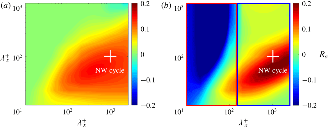
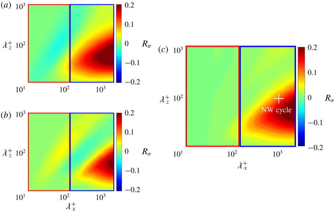
Figure 2 shows resolvent-based predictions for case SP and case ST with
 $\unicode[STIX]{x1D6FC}^{+}=0.5$
and
 $\unicode[STIX]{x1D6FC}^{+}=10$
, respectively. Both panels show the normalized change in squared singular values relative to the uncontrolled case. We consider this measure, which represents the predicted change in energy amplification, to be a surrogate for drag reduction. For each wavenumber combination
 $(k_{x},k_{z})$
, the ratio of squared singular values is integrated over the range of wave speeds
 $0\leqslant c\leqslant 1$
, where
 $c$
is normalized by the centreline velocity (Nakashima et al.
Reference Nakashima, Fukagata and Luhar2017). In other words, the predicted ‘drag reduction’ rate across wavenumber space is defined as
 $$\begin{eqnarray}R_{\unicode[STIX]{x1D70E}}(k_{x},k_{z})=1-\frac{\displaystyle \int _{0}^{1}\unicode[STIX]{x1D70E}_{\boldsymbol{k}c}^{2}(k_{x},k_{z},c)\,\text{d}c}{\displaystyle \int _{0}^{1}\unicode[STIX]{x1D70E}_{\boldsymbol{k}0}^{2}(k_{x},k_{z},c)\,\text{d}c}.\end{eqnarray}$$
The cross markers in figure 2 represent length scales that characterize the NW cycle,
 $\unicode[STIX]{x1D706}_{x}^{+}\approx 10^{3}$
and
 $\unicode[STIX]{x1D706}_{z}^{+}\approx 10^{2}$
. Note that the maximum wavelengths shown in this figure correspond to the DNS domain size,
 $\unicode[STIX]{x1D706}_{x}^{+}\leqslant 4\unicode[STIX]{x03C0}\unicode[STIX]{x1D6FF}^{+}$
and
 $\unicode[STIX]{x1D706}_{z}^{+}\leqslant 2\unicode[STIX]{x03C0}\unicode[STIX]{x1D6FF}^{+}$
.
As shown in figure 2(a), resolvent analysis predicts mode suppression (i.e.
 $1-(\unicode[STIX]{x1D70E}_{\boldsymbol{k}c}/\unicode[STIX]{x1D70E}_{\boldsymbol{k}0})^{2}>0$
) for case SP over a wide region of spectral space. Singular values are nearly unchanged in regions where drag reduction is not expected. Based on this prediction, we hypothesize that a spatial wavenumber filter is unlikely to yield a substantial difference in performance. DNS for case SP with control over all streamwise wavelengths yielded approximately 15 % drag reduction in the present study, which is a little smaller than the value reported by Lee et al. (Reference Lee, Kim and Choi1998). This is probably due to the slight increase in Reynolds number. According to Iwamoto et al. (Reference Iwamoto, Suzuki and Kasagi2002), suboptimal control becomes less effective in reducing the skin friction when the friction Reynolds number increases. For instance, drag reduction decreases from 20 % at
 $Re_{\unicode[STIX]{x1D70F}}=110$
to 15 % at
 $Re_{\unicode[STIX]{x1D70F}}=150$
. Since Lee et al. (Reference Lee, Kim and Choi1998) obtained
 ${>}20\,\%$
drag reduction at
 $Re_{\unicode[STIX]{x1D70F}}=110$
, the slightly lower value obtained here at
 $Re_{\unicode[STIX]{x1D70F}}=180$
is consistent with prior results.
Resolvent-based predictions for singular-value suppression at
 $Re_{\unicode[STIX]{x1D70F}}=180$
for (a) case SP (
 $\unicode[STIX]{x1D6FC}^{+}=0.5$
) and (b) case ST (
 $\unicode[STIX]{x1D6FC}^{+}=10$
).

Figure 2(b) shows resolvent-based predictions for case ST. Unlike case SP, for this case, the effects of control vary significantly across spectral space. For modes with streamwise length scales larger than
 $\unicode[STIX]{x1D706}_{x}^{+}\approx 200$
, the singular-value ratio is suppressed by 10–20 %. For shorter modes with streamwise length scales smaller than
 $\unicode[STIX]{x1D706}_{x}^{+}\approx 200$
, the singular-value ratio increases substantially.
In the original simulations, Lee et al. (Reference Lee, Kim and Choi1998) reported that case ST leads to an increase in drag. The model predictions shown in figure 2(b) suggest that drag reduction may be attained if a spatial wavenumber is employed such that control is implemented only over the long-wavelength region. Based on these predictions, we pursued three separate DNS cases, with: (i) control applied only for structures with long streamwise wavelengths,
 $\unicode[STIX]{x1D706}_{x}^{+}\geqslant 140$
, for which resolvent analysis predicts mode suppression, i.e. the region enclosed by the blue box in figure 2(b); (ii) control applied only for short streamwise wavelengths,
 $\unicode[STIX]{x1D706}_{x}^{+}<140$
, for which resolvent analysis predicts further amplification, i.e. the region enclosed by the red box in figure 2(b); and (iii) with control applied over all scales, which corresponds to the baseline case ST studied previously. Hereafter, these three cases are termed ST-CL, ST-CS and ST-CA, respectively. Note that in the present study, the term ‘large scales’ is used to denote the NW cycle, not the much larger structures that emerge at higher Reynolds numbers and are multiple outer units in length (e.g. the so-called large-scale and very-large-scale motions (see Smits, McKeon & Marusic Reference Smits, McKeon and Marusic2011)).
Drag reduction rates
 $R_{D}$
(%) obtained in DNS.

Interestingly, none of these three cases showed a substantial change in drag. As summarized in table 2, DNS for case ST-CL only shows a small amount of drag reduction (
 $R_{D}=1.2\,\%$
) while case ST-CS leads to no perceptible change in drag (
 $R_{D}=0.06\,\%$
). To evaluate why these DNS results contradict resolvent-based predictions, we revisit the blowing-and-suction parameter,
 $\unicode[STIX]{x1D6FC}^{+}$
, imposed in our DNS. As noted earlier, the value
 $\unicode[STIX]{x1D6FC}^{+}=10$
was estimated from previous DNS results based on the assumption that the NW cycle is the dominant flow feature close to the wall. Specifically, equation (2.6) was rearranged to yield
 $$\begin{eqnarray}\unicode[STIX]{x1D6FC}^{+}\approx \frac{K}{k_{x}}\frac{\unicode[STIX]{x1D719}_{rms}^{+}}{(\unicode[STIX]{x2202}u_{rms}/\unicode[STIX]{x2202}y)_{w}^{+}}\approx 10\frac{\unicode[STIX]{x1D719}_{rms}^{+}}{(\unicode[STIX]{x2202}u_{rms}/\unicode[STIX]{x2202}y)_{w}^{+}},\end{eqnarray}$$
under the assumption that
 $K/k_{x}\approx k_{z}/k_{x}=10$
. For case ST-CA, the magnitudes of streamwise wall shear stress and control input were
 $(\unicode[STIX]{x2202}u/\unicode[STIX]{x2202}y)_{w}^{+}\approx 0.4$
and
 $\unicode[STIX]{x1D719}_{rms}^{+}=0.25$
, respectively, in the DNS conducted here. Thus, if the NW cycle is the dominant contributor in the expression above and
 $K/k_{x}\approx 10$
, the a priori estimate
 $\unicode[STIX]{x1D6FC}^{+}\sim O(10)$
is reasonable. Indeed, Nakashima et al. (Reference Nakashima, Fukagata and Luhar2017) showed similar arguments to be valid for suboptimal control based on the spanwise wall shear stress (case SP).
To estimate the true value of
 $\unicode[STIX]{x1D6FC}^{+}$
imposed in the present DNS for case ST-CA, based on the condition that
 $\unicode[STIX]{x1D719}_{rms}=v_{rms,0}(y^{+}\approx 10)$
, we follow the following procedure. First, we compute the ‘unscaled’ value for the blowing-and-suction magnitude in Fourier space, as
 $$\begin{eqnarray}\hat{\unicode[STIX]{x1D719}}_{\unicode[STIX]{x1D6FC}}=-\frac{\text{i}k_{x}}{K}\left(\widehat{\frac{\unicode[STIX]{x2202}u}{\unicode[STIX]{x2202}y}}\right)_{w}.\end{eqnarray}$$
Next, this unscaled value for the actuation is inverse-Fourier-transformed and its r.m.s. value,
 $\unicode[STIX]{x1D719}_{\unicode[STIX]{x1D6FC},rms}$
, is computed in physical space. Finally, the effective value for
 $\unicode[STIX]{x1D6FC}$
is estimated from the ratio
 $$\begin{eqnarray}\unicode[STIX]{x1D6FC}\approx \frac{v_{rms,0}(y^{+}\approx 10)}{\unicode[STIX]{x1D719}_{\unicode[STIX]{x1D6FC},rms}}.\end{eqnarray}$$
Estimates based on this procedure suggest a range,
 $\unicode[STIX]{x1D6FC}^{+}\in [0.2,1.0]$
, that is much smaller than the assumed value,
 $\unicode[STIX]{x1D6FC}^{+}=10$
. This indicates that the assumption
 $K/k_{x}\approx 10$
in (3.3) is inaccurate, and that the NW cycle is not the sole dominant flow feature when it comes to estimating the fluctuating streamwise wall shear stress in turbulent channel flow.
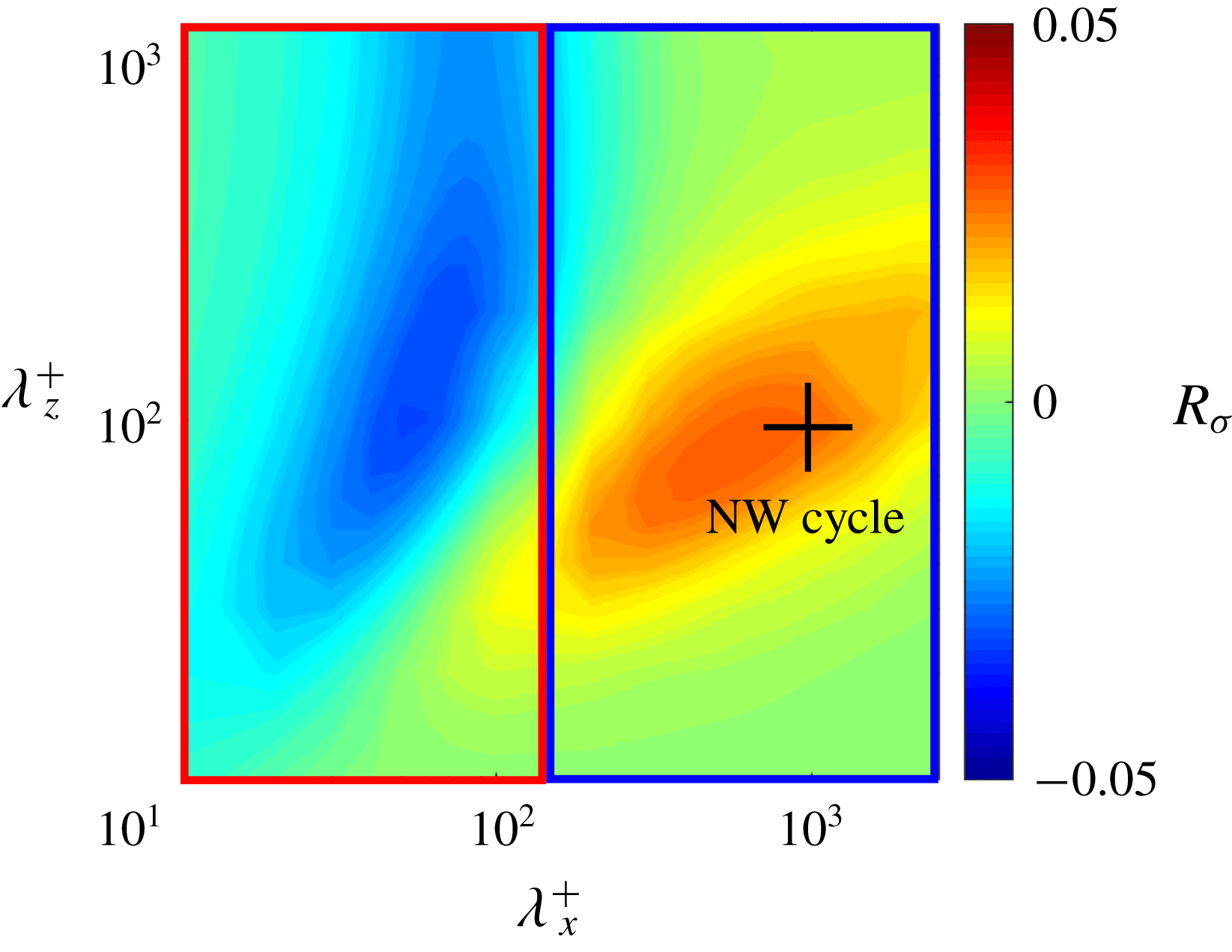
Resolvent-based predictions for singular-value suppression at
 $Re_{\unicode[STIX]{x1D70F}}=180$
for case ST with
 $\unicode[STIX]{x1D6FC}^{+}=0.5$
.

For completeness, figure 3 shows resolvent-based predictions for mode amplification across spectral space under case ST with the modified blowing-and-suction parameter,
 $\unicode[STIX]{x1D6FC}^{+}=0.5$
. Compared to the predictions shown in figure 2(b) for
 $\unicode[STIX]{x1D6FC}^{+}=10$
, the predicted changes in mode amplification are much smaller. For instance, the suppression predicted for modes with length scales corresponding to the NW cycle is
 $R_{\unicode[STIX]{x1D70E}}\approx 0.03$
for
 $\unicode[STIX]{x1D6FC}^{+}=0.5$
, which is a factor of five lower than the suppression predicted for
 $\unicode[STIX]{x1D6FC}^{+}=10$
. This suggests that case ST-CL does not lead to substantial drag reduction in DNS due to the relatively weak blowing-and-suction magnitude. Similarly, the lack of substantial mode amplification for
 $\unicode[STIX]{x1D706}_{x}^{+}<140$
at
 $\unicode[STIX]{x1D6FC}^{+}=0.5$
also explains why case ST-CS does not lead to a significant increase in drag.
The above discussion suggests that increasing the actuation amplitude for case ST-CL could result in drag reduction, albeit with increased actuation cost. However, additional DNS for case ST-CL with
 $\unicode[STIX]{x1D719}_{rms}^{+}=0.5$
or
 $1$
(two or four times the original actuation strength) did not yield substantial increases in drag reduction. Nevertheless, even with this increased actuation, values for the blowing-and-suction parameter were still well below the
 $\unicode[STIX]{x1D6FC}^{+}\approx 10$
estimate used to generate the predictions shown in figure 2(b).
In sum, suboptimal control for case ST does not lead to observable changes in the present DNS due to the relatively low value of
 $\unicode[STIX]{x1D6FC}$
; resolvent analysis only predicts marginal changes in mode amplification for
 $\unicode[STIX]{x1D6FC}^{+}=0.5$
. In other words, the failure of case ST at reducing drag in the present DNS is caused not just by the detrimental effect on small scales (as hypothesized by Nakashima et al. (Reference Nakashima, Fukagata and Luhar2017)), but also due to the very low actuation amplitude. Note that we also estimated
 $\unicode[STIX]{x1D6FC}$
for case SP using the procedure described above and again obtained
 $\unicode[STIX]{x1D6FC}^{+}\sim O(0.1)$
. Thus, it appears that
 $\unicode[STIX]{x1D6FC}^{+}\sim O(0.1)$
is a robust estimate for suboptimal control in which
 $\unicode[STIX]{x1D719}_{rms}=v_{rms,0}(y^{+}\approx 10)$
. In the following section, we propose new control laws based on the insights gained here, assuming
 $\unicode[STIX]{x1D6FC}^{+}=0.5$
for the purposes of resolvent analysis.
3.2 Proposal of new control laws
The DNS results and resolvent-based predictions presented in the previous section suggest the following key insights for suboptimal control based on the streamwise wall shear stress. First, resolvent analysis predicts that control performance is mixed in spectral space. Structures with large streamwise length scales (low
 $k_{x}$
) are suppressed by control while shorter structures may be further amplified. Second, with the scaling factor
 $\unicode[STIX]{x1D6FC}(k_{x}/K)$
in (2.6) and the requirement that
 $\unicode[STIX]{x1D719}_{rms}=v_{rms,0}(y^{+}\approx 10)$
, the magnitude of blowing and suction is too weak for control to have a substantial effect on the energetic NW cycle.
Based on these observations, we propose new feedback control laws. Specifically, we retain the reliance on streamwise wall shear stress measurements (this is desirable from a practical viewpoint), but change the scaling factor in (2.6) from
 $\unicode[STIX]{x1D6FC}(k_{x}/K)$
to
 $\unicode[STIX]{x1D6FC}(k_{z}/K)$
. This effectively increases blowing and suction for longer structures with low streamwise wavenumber such as the NW cycle, and decreases the actuation for shorter structures that are predicted to be further amplified under control per figure 2(b). Actually, replacing
 $k_{x}$
with
 $k_{z}$
in the case ST control law leads to a 50–100 % suppression in the actuation amplitude for the spectral region with
 $\unicode[STIX]{x1D706}_{x}^{+}<140$
and a roughly 100 % increase in actuation amplitude for the larger scales. Two candidate control laws are
 $$\begin{eqnarray}\displaystyle \text{(case STz)}:\qquad \hat{\unicode[STIX]{x1D719}}=-\unicode[STIX]{x1D6FC}\frac{\text{i}k_{z}}{K}\left(\widehat{\frac{\unicode[STIX]{x2202}u}{\unicode[STIX]{x2202}y}}\right)_{w} & & \displaystyle\end{eqnarray}$$
and
 $$\begin{eqnarray}\displaystyle \text{(case STrz)}:\qquad \hat{\unicode[STIX]{x1D719}}=+\unicode[STIX]{x1D6FC}\frac{\text{i}k_{z}}{K}\left(\widehat{\frac{\unicode[STIX]{x2202}u}{\unicode[STIX]{x2202}y}}\right)_{w}. & & \displaystyle\end{eqnarray}$$
Since multiplication by
 $k_{z}$
in Fourier space denotes a differentiation in the spanwise direction, these new control laws may also be interpreted as modified versions of the discrete formulation identified by Morimoto et al. (Reference Morimoto, Iwamoto, Suzuki and Kasagi2002) using a genetic algorithm,
 $$\begin{eqnarray}\unicode[STIX]{x1D719}=\unicode[STIX]{x1D6FC}\left[\left.\frac{\unicode[STIX]{x2202}u}{\unicode[STIX]{x2202}y}\right|_{w}(x^{+},z^{+}+20)-\left.\frac{\unicode[STIX]{x2202}u}{\unicode[STIX]{x2202}y}\right|_{w}(x^{+},z^{+}-20)\right].\end{eqnarray}$$
Note that, unlike cases SP and ST, the newly proposed laws introduce a spanwise asymmetry depending on the sign of
 $k_{z}$
. Specifically, the actuation changes for modes with
 $k_{z}<0$
relative to that for modes with
 $k_{z}>0$
. Further, case STz has the same control effect on modes with
 $k_{z}>0$
as case STrz does on modes with
 $k_{z}<0$
, and vice versa. These spanwise asymmetries in the new control laws are confirmed by the resolvent-based predictions shown in figure 4. Figures 4(a) and 4(b) show predicted singular-value ratios for modes with
 $k_{z}>0$
for case STz and case STrz, respectively. It has also been confirmed that, for modes with
 $k_{z}<0$
, the predictions are reversed, i.e. figure 4(a) corresponds to case STrz, while figure 4(b) corresponds to case STz. Of course, if contributions from both oblique modes,
 $k_{z}>0$
and
 $k_{z}<0$
, are combined, resolvent analysis predicts identical control effects for cases STz and STrz. Predicted mode suppression for this scenario is shown in figure 4(c).
Resolvent-based predictions for singular-value suppression at
 $\unicode[STIX]{x1D6FC}^{+}=0.5$
for: (a) case STz (
 $k_{z}>0$
); (b) case STrz (
 $k_{z}>0$
); and (c) case STz and case STrz when both
 $k_{z}>0$
and
 $k_{z}<0$
are considered.

Importantly, figure 4(c) shows that both case STz and case STrz overcome the drawbacks associated with case ST. Namely, singular values are suppressed substantially in the spectral region corresponding to the NW cycle at
 $\unicode[STIX]{x1D6FC}^{+}=0.5$
, with
 $R_{\unicode[STIX]{x1D70E}}\approx 0.1$
. Further, in contrast to the predictions shown in figure 2(b), there are very limited detrimental effects on modes with short streamwise length scales.
3.3 Evaluation of new control laws
To test these predictions, we conducted DNS with the new control laws with, and without, spatial filtering. The observed performance for both cases STz and STrz was consistent with predictions made using resolvent analysis. Approximately 10 % drag reduction was obtained without the spatial filtering (CA) and for the case in which control was limited to large streamwise wavelengths (CL). Almost no effect was observed when control was limited to short streamwise wavelengths (CS). Moreover, there were no statistically significant differences between case STz and case STrz. Table 2 provides a summary of the total drag reduction observed in DNS for all the control laws (ST, STz, STrz) and spatial filters (CA, CL, CS) considered here.
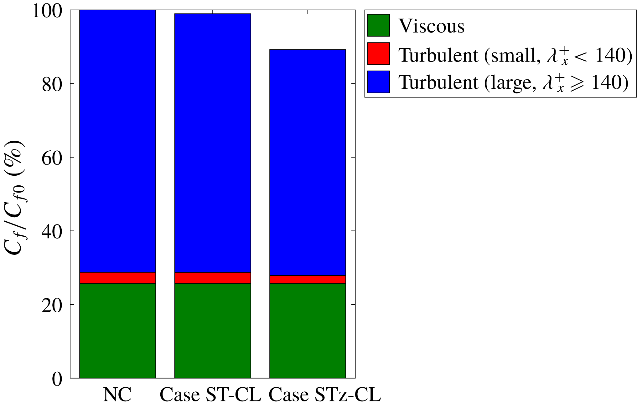
To further evaluate the efficacy of the new control laws, the large- and small-scale contributions to total skin friction were quantified using the Fukagata–Iwamoto–Kasagi (FIK) identity (Fukagata et al. Reference Fukagata, Iwamoto and Kasagi2002):
 $$\begin{eqnarray}\displaystyle C_{f}=\frac{12}{Re_{b}}+12\int _{0}^{1}2(1-y)(-\overline{u^{\prime }v^{\prime }})\,\text{d}y. & & \displaystyle\end{eqnarray}$$
Here, all variables are made dimensionless using the channel half-width,
 $\unicode[STIX]{x1D6FF}$
, and twice the bulk mean velocity,
 $2U_{b}$
. The second term in (3.9), which represents the turbulent contribution to the skin friction coefficient, was decomposed into two components in a manner similar to Fukagata, Kobayashi & Kasagi (Reference Fukagata, Kobayashi and Kasagi2010): the large-scale contribution from structures with
 $\unicode[STIX]{x1D706}_{x}^{+}\geqslant 140$
, and the small-scale contribution from structures with
 $\unicode[STIX]{x1D706}_{x}^{+}<140$
. This decomposition shows that, in case STz-CL, the large-scale contribution to the total skin friction decreases from 71 % for the uncontrolled case to 61 % (figure 5), which constitutes the majority of the 11 % total drag reduction obtained under cases STz-CA and STz-CL (table 2). Together, these results confirm that the suppression of large-scale structures with
 $\unicode[STIX]{x1D706}_{x}^{+}\geqslant 140$
is central to the drag reduction obtained under cases STz and STrz, which is consistent with resolvent-based predictions.
Contribution to friction drag for the uncontrolled case, case ST-CL and case STz-CL.

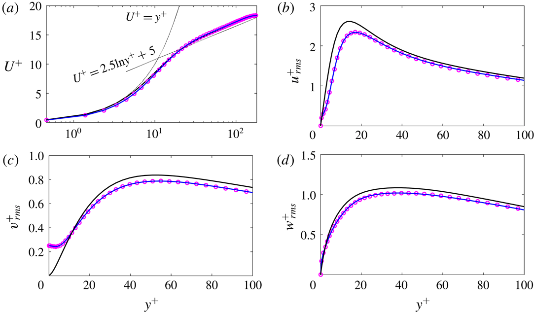
Results obtained in DNS. (a) The mean velocity profile. Profiles for the (b) r.m.s. fluctuating streamwise velocity
 $u_{rms}^{+}$
, (c) wall-normal velocity
 $v_{rms}^{+}$
, and (d) spanwise velocity
 $w_{rms}^{+}$
. Black line, uncontrolled case; blue line, case STz-CL; magenta circles, case STz-CA.

Figure 6(a–d) shows the profiles of mean streamwise velocity and r.m.s. fluctuating velocities obtained in DNS. For the uncontrolled case, all the profiles (black lines) are consistent with known features of wall-bounded turbulent flows. The mean velocity profile shows a linear increase in the viscous sublayer and the presence of a logarithmic region further from the wall. The r.m.s. velocity profiles show good agreement with previous spectral DNS results (Moser, Kim & Mansour Reference Moser, Kim and Mansour1999). For the controlled cases, it is clear that cases STz-CA (magenta circles) and STz-CL (blue lines) show nearly identical profiles for these mean turbulence statistics. This essentially means that the new control laws produce the same effect with and without the low-pass spatial filter.
The viscous normalization employed in figure 6 corresponds to the friction velocity for the uncontrolled case. With this in mind, the slight decrease in near-wall
 $U^{+}$
observed for the controlled cases in figure 6(a) is consistent with a reduction in skin friction, i.e. the decrease in near-wall
 $U$
represents a decrease in the wall shear stress
 $\unicode[STIX]{x1D70F}_{w}=\unicode[STIX]{x1D707}\,\text{d}U/\text{d}y$
. In addition, as shown in figure 6(b–d), the r.m.s. values of all velocity components decrease across the channel, which is consistent with a decrease in turbulence intensity. For instance, the peak value of
 $u_{rms}$
decreases by approximately 10 % for both case STz-CA and case STz-CL. These observations are consistent with previously reported DNS results for effective controls (e.g. Deng et al.
Reference Deng, Huang and Xu2016).
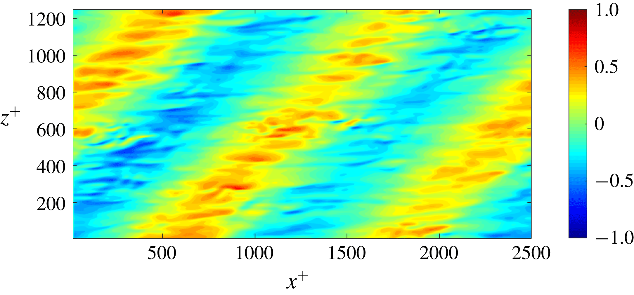
Distribution of the instantaneous control input,
 $\unicode[STIX]{x1D719}^{+}$
, for case STz-CA at
 $t^{+}\approx 900$
after control begins.

Figure 7 shows the instantaneous spatial distribution of blowing and suction,
 $\unicode[STIX]{x1D719}^{+}$
, for case STz-CA at
 $t^{+}\approx 900$
after control commences. The spatial distribution of
 $\unicode[STIX]{x1D719}^{+}$
shows a distinct domain-scale periodic pattern (i.e. with
 $\unicode[STIX]{x1D706}_{x}=L_{x}/2$
and
 $\unicode[STIX]{x1D706}_{z}=L_{z}$
) with alternating regions of blowing (
 $\unicode[STIX]{x1D719}^{+}>0$
) and suction (
 $\unicode[STIX]{x1D719}^{+}<0$
) that are tilted in the streamwise–spanwise plane. Similar patterned control inputs have also been reported in other feedback control schemes (Koumoutsakos Reference Koumoutsakos1999; Hasegawa & Kasagi Reference Hasegawa and Kasagi2011), though these previous simulations did not yield oblique structures.
Additional tests indicate that the oblique structures observed here are most likely a numerical artifact arising from the limited size of the computational domain. Specifically, when the computational domain is reduced by a factor of two, the size of the oblique structures is also halved. Moreover, these structures do not appear to play an important role in terms of drag reduction. Statistically, the control effect does not change if the amplitude coefficient for the wavenumber combination corresponding to
 $(\unicode[STIX]{x1D706}_{x},\unicode[STIX]{x1D706}_{z})=(L_{x}/2,L_{z})$
is artificially set to zero. In any case, the phase speed associated with these patterned inputs is too high (
 $c^{+}\simeq 800$
) to allow for dynamic interaction with the turbulent structures arising in the flow. Although the emergence of these oblique periodic patterns needs to be investigated further, the tests described above indicate that the structures seen in figure 7 do not contribute substantially to drag reduction. An alternative drag reduction mechanism for cases STz and STrz is proposed in § 4.
Instantaneous distribution of the streamwise velocity fluctuations,
 ${u^{\prime }}^{+}$
, in the
 $x$
–
 $z$
plane at
 $t^{+}\approx 900$
after control commences: (a,c,e) uncontrolled case; (b,d,f) case STz-CA; (a,b)
 $y^{+}\approx 3$
; (c,d)
 $y^{+}\approx 5$
; (e,f)
 $y^{+}\approx 15$
.

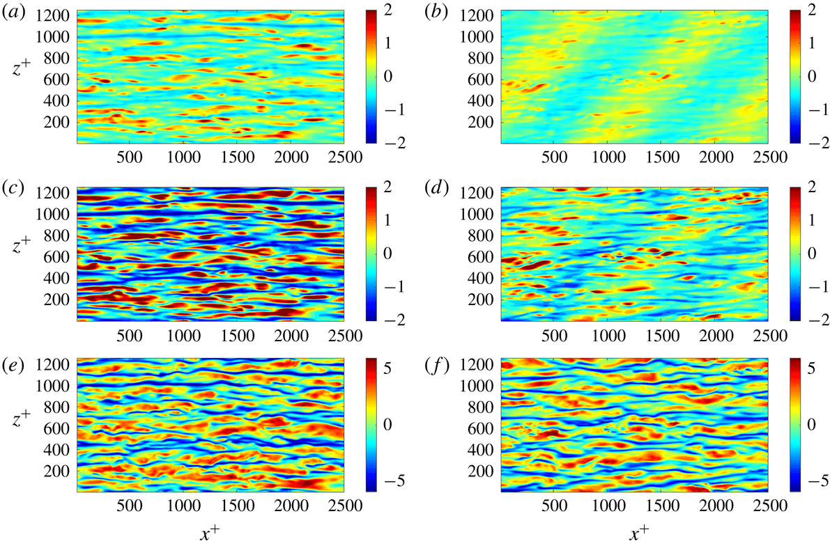
Figure 8 shows that the present control input suppresses the formation of streamwise velocity streaks in the near-wall region. As is typical for the NW cycle, the uncontrolled case shows the presence of elongated high- and low-speed streaks aligned in the streamwise direction (figure 8
a,c,e). For case STz, figure 8(b,d) shows that these streaks are damped substantially at
 $y^{+}\approx 3$
and
 $y^{+}\approx 5$
. A qualitative comparison between the uncontrolled and controlled cases in figure 8 also suggests that, in the presence of control, the near-wall streaks show an oblique bias. Specifically, there appear to be more streaks inclined in the positive
 $z$
-direction (from bottom-left to top-right in these panels) compared to the negative
 $z$
-direction.
To test for this non-equivalence between modes with
 $k_{z}>0$
and
 $k_{z}<0$
under case STz, we computed two-dimensional (2D) Fourier transforms for the snapshots shown in figure 8(b,d,f). Fourier transforms for these snapshots confirm that, for
 $k_{x}>0$
, streamwise velocity fluctuations with
 $k_{z}<0$
are more energetic than fluctuations with
 $k_{z}>0$
, i.e. streaks inclined in the positive
 $z$
-direction are suppressed less under control (data not shown here). Note that this observation is consistent with the asymmetric control effect predicted by resolvent analysis for NW-type modes (see figure 4
a,b). Singular values associated with the NW modes are reduced from
 $\unicode[STIX]{x1D70E}_{\boldsymbol{k}0}(k_{z}>0)=\unicode[STIX]{x1D70E}_{\boldsymbol{k}0}(k_{z}<0)=3.6$
for the uncontrolled case to
 $\unicode[STIX]{x1D70E}_{\boldsymbol{k}c}(k_{z}>0)=2.8$
and
 $\unicode[STIX]{x1D70E}_{\boldsymbol{k}c}(k_{z}<0)=3.2$
for case STz. In other words, control leads to greater suppression for modes with
 $k_{z}>0$
. The physical mechanism creating this asymmetry in control efficacy for modes with
 $k_{z}<0$
and
 $k_{z}>0$
is discussed in § 4.2.
Premultiplied 2D co-spectra at
 $y^{+}=5$
: (a–c)
 $E_{uu}$
; (d–f)
 $E_{vv}$
; and (g–i)
 $E_{ww}$
. Cases: (a,d,g) uncontrolled case; (b,e,h) case ST-CA; and (c,f,i) case STz-CA.

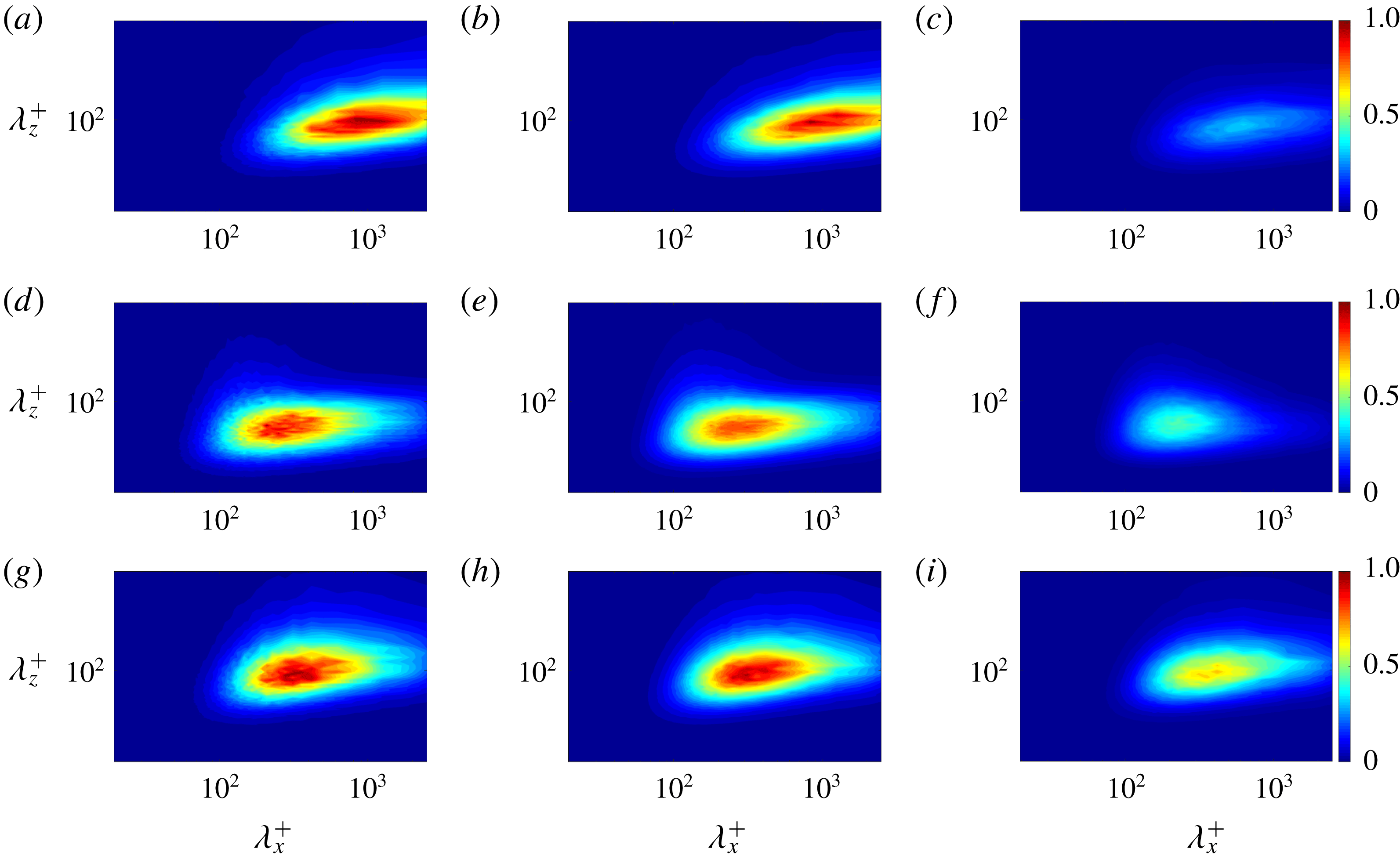
Figure 9 shows the 2D premultiplied co-spectra for the streamwise (
 $E_{uu}$
), wall-normal (
 $E_{vv}$
) and spanwise velocity (
 $E_{ww}$
) at
 $y^{+}=5$
obtained from DNS for the uncontrolled case, case ST-CA and case STz-CA. Each co-spectrum is normalized by the maximum value for the uncontrolled case. Figure 9(a,d,g) confirm that the results obtained here for the uncontrolled case are consistent with the spectra observed in previous DNS. The streamwise spectrum
 $E_{uu}$
shows a clear peak at the wavelength combination corresponding to the NW cycle. Spectra for the wall-normal and spanwise velocity show peaks at slightly lower streamwise wavelengths.
For case STz-CA, spectra for all velocity components show substantial damping, though this is especially apparent for the streamwise component (see figure 9(c,f,i)). The reduction in
 $E_{uu}$
confirms the suppression of near-wall streaks that was evident in figure 8. Similarly, reduction in
 $E_{vv}$
and
 $E_{ww}$
indicates that the quasi-streamwise vortices associated with the NW cycle are also substantially damped. Together, a suppression of spectra for all three velocity components implies a reduction in turbulent kinetic energy, which is directly related to drag reduction. In contrast to the spectra obtained for case STz-CA, spectra for case ST-CA show very little change relative to the uncontrolled case. This is consistent with the marginal reduction in drag obtained for case ST-CA (table 2). Note that the observations for case ST-CA and case STz-CA described above also hold for the case in which control is applied only for long wavelengths (i.e. for cases ST-CL and STz-CL).
To examine the change in
 $E_{uu}$
,
 $E_{vv}$
and
 $E_{ww}$
more quantitatively, we integrate these spectra over all wall-normal locations as well as specified regions of spectral space, and compute integrated reduction rates relative to the controlled flow. As an example, the reduction rate for the streamwise component is defined as
 $$\begin{eqnarray}\displaystyle R_{uu}=1-\frac{\displaystyle \iiint E_{uu,c}(k_{x},y,k_{z})\,\text{d}k_{x}\,\text{d}y\,\text{d}k_{z}}{\displaystyle \iiint E_{uu,0}(k_{x},y,k_{z})\,\text{d}k_{x}\,\text{d}y\,\text{d}k_{z}}. & & \displaystyle\end{eqnarray}$$
Table 3 shows the integrated reduction rates obtained under cases ST-CA and STz-CA for all three components (
 $R_{uu},R_{vv},R_{ww}$
). Note that three different sets of values are shown, corresponding to integrals over (i) all streamwise wavelengths, (ii) only large streamwise wavelengths,
 $\unicode[STIX]{x1D706}_{x}^{+}\geqslant 140$
, and (iii) only small streamwise wavelengths,
 $\unicode[STIX]{x1D706}_{x}^{+}<140$
.
For case ST-CA, the reduction rates obtained are small (
 ${\lesssim}2\,\%$
) for all components of velocity and over all length scales. This is consistent with the marginal decrease in average skin friction observed in DNS. Further, the reduction rates are lowest for structures with small streamwise wavelengths, for which resolvent analysis predicts a small increase in mode amplification (figure 3). For case STz-CA, the integrated reduction rates over the long-wavelength region for all components of velocity are approximately 15 %, which is broadly consistent with the resolvent-based predictions for mode amplification presented in figure 4(c). Interestingly, integrated reduction rates over the short-wavelength region (
 $\unicode[STIX]{x1D706}_{x}^{+}<140$
) for all components of velocity are higher, approximately 20 %. Resolvent analysis for case STz does not predict substantial mode suppression over this region, indicating that the observed suppression of these smaller structures is due to nonlinear energy transfer. Specifically, these results suggest that weakening of larger-scale turbulent structures inhibits the cascade of turbulent kinetic energy down to small scales. In the resolvent formalism, these nonlinear effects would result in a reduction of the forcing term for smaller structures. As a result, the forcing normalized analysis of mode suppression considered here is unable to predict a suppression of small-scale turbulence.
Integrated reduction rates for all velocity components obtained in DNS for cases ST-CA and STz-CA (
 $\%$
).

4 Discussion
The previous sections have shown that the modified control laws, cases STz and STrz, are able to successfully reduce turbulent skin friction. In this section, we evaluate the effects of these new control laws on the near-wall dynamics (§ 4.1) and propose a physical interpretation (§ 4.2).
4.1 Near-wall dynamics
First, we study how the new control laws developed above affect the near-wall flow field in DNS, focusing on case STz. Figure 8 shows that case STz leads to a substantial damping of near-wall streaks. These streaks arise from the wall-normal transport of streamwise momentum by the QSVs associated with the near-wall cycle. To examine how control affects these QSVs, we employ conditional averaging. Specifically, we compare conditionally averaged (
 $y,z$
) cross-sections of the vortices in the controlled flow with those in the uncontrolled flow.
4.1.1 Conditional averaging method
The vortex eduction scheme employed here is conceptually similar to the process used by Jeong et al. (Reference Jeong, Hussain, Schoppa and Kim1997). There are two basic steps involved in the extraction of representative vortex structures from instantaneous snapshots of the flow field. First, QSVs must be identified in each snapshot and then averaged in the streamwise direction to generate a 2D representation in the
 $y$
–
 $z$
plane. This procedure, referred to as phase I for the remainder of this section, is non-trivial since the vortices are not perfectly aligned in the
 $x$
-direction. Second, all 2D vortices identified in phase I that exist at the same height above the wall are time-averaged. This is referred to as phase II.
In phase I, QSVs are identified based on the
 $Q$
-criterion, defined as
 $Q=\unicode[STIX]{x1D61A}_{ij}\unicode[STIX]{x1D61A}_{ji}-\unicode[STIX]{x1D6FA}_{ij}\unicode[STIX]{x1D6FA}_{ji}$
. Here,
 $\unicode[STIX]{x1D61A}_{ij}$
and
 $\unicode[STIX]{x1D6FA}_{ij}$
are, respectively, the symmetric and antisymmetric components of the velocity gradient tensor (Hunt, Wray & Moin Reference Hunt, Wray and Moin1988). We detect locations corresponding to the minimum value of
 $Q$
in each
 $y$
–
 $z$
plane (note that these locations represent regions of high rotation), and plot the spanwise variation of these minima along the
 $x$
-axis. In other words, we track the locations of these minima in the
 $x$
–
 $z$
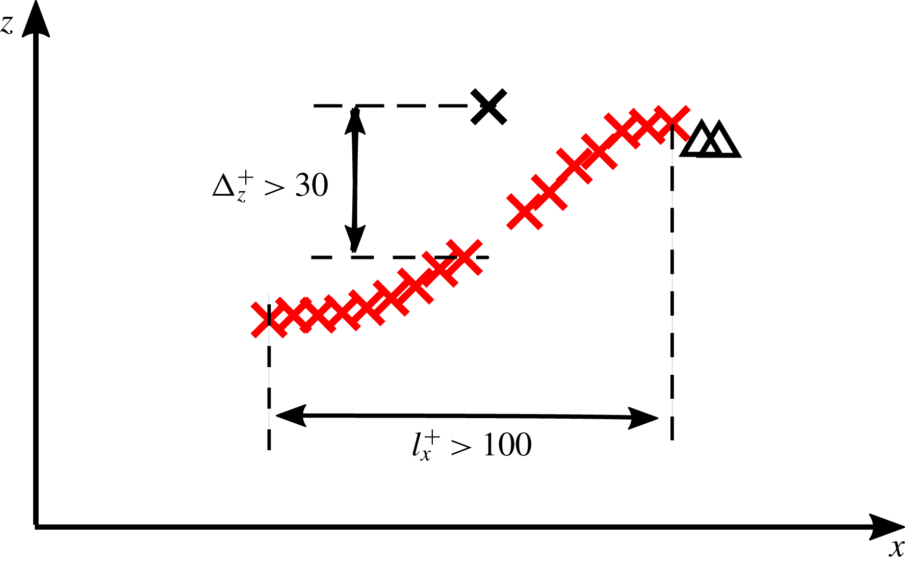
plane, as shown in figure 10. The line connecting these local minima of
 $Q$
in the
 $x$
–
 $z$
plane is considered to be the axis of the QSVs. Points regarded as part of the same QSV are chosen based on the following three conditions: (i) the sign of the streamwise vorticity at these locations must be identical (i.e. the vortices must have the same sense of rotation); (ii) the streamwise length of the line must be
 $l_{x}^{+}>100$
; and (iii) the spanwise shift between adjacent streamwise planes must be
 $\unicode[STIX]{x0394}z^{+}<30$
. Condition (ii) ensures that the vortices identified are coherent in the streamwise direction, while conditions (i) and (iii) ensure that neighbouring vortex structures are not misidentified as being part of the same QSV. The numerical thresholds used for these conditions were chosen based on previous observations, which indicate that the streamwise length of QSVs is
 $l_{x}^{+}\approx 150{-}300$
and the vortex diameter is typically
 $d^{+}\approx 20$
–50 (Kim et al.
Reference Kim, Moin and Moser1987).
Schematic describing the conditional averaging method. Crosses denote points with
 $\unicode[STIX]{x1D714}_{x}^{+}>0$
while triangles denote points with
 $\unicode[STIX]{x1D714}_{x}^{+}<0$
. Flow fields corresponding to the red markers are identified as being part of the same vortex and retained for conditional averaging, while flow fields corresponding to the black markers are excluded from the averaging procedure.

Figure 10 shows a schematic describing the phase I detection process for a vortex with positive streamwise vorticity,
 $\unicode[STIX]{x1D714}_{x}^{+}>0$
. In this figure, the cross and triangle markers represent locations of minimum
 $Q$
, but with positive and negative
 $\unicode[STIX]{x1D714}_{x}^{+}$
, respectively. Red markers are regarded as being a part of the same vortex. The black markers are discarded because they do not satisfy the conditions (i)–(iii) described above. For example, the black cross marker is eliminated since the spanwise distance from the vortex of interest is too far, and the black triangle markers are excluded because the direction of rotation is inconsistent with the targeted vortex.
Next, flow fields identified as being part of the same vortex are aligned (i.e. shifted in the spanwise direction), and averaged in the streamwise direction to generate a representative 2D flow field in the
 $y$
–
 $z$
plane for this snapshot. The wall-normal location of the core for the resulting QSV is defined as the location that has the lowest value of
 $Q$
. Subsequently, in phase II, we ensemble average the 2D vortices collected from each instantaneous flow field. In this step, we only average together vortices with cores located at the same height above the wall.
The conditionally averaged flow fields shown below are extracted from
 $150$
instantaneous snapshots obtained at time intervals of
 $\unicode[STIX]{x0394}t^{+}\approx 30$
. Since the vortex eduction process is time- and data-intensive, flow fields from a smaller computational domain (
 $2\unicode[STIX]{x03C0}\times 2\times \unicode[STIX]{x03C0}$
, see table 1) are employed. It has been verified that results for case STz do not change substantially in this smaller domain.
For the uncontrolled flow, 23 anticlockwise (counterclockwise) vortices (CCW;
 $\unicode[STIX]{x1D714}_{x}^{+}<0$
) and 22 clockwise vortices (CW;
 $\unicode[STIX]{x1D714}_{x}^{+}>0$
) were identified and averaged together. For case STz, 23 CCW and 26 CW vortices were identified and averaged. For both CCW and CW conditionally averaged vortices, the cores were located at
 $y^{+}\approx 22{-}24$
. Conditionally averaged flow fields for vortices at slightly different heights show qualitatively similar behaviour (results not shown here).
4.1.2 Comparison of conditionally averaged flow fields and resolvent modes
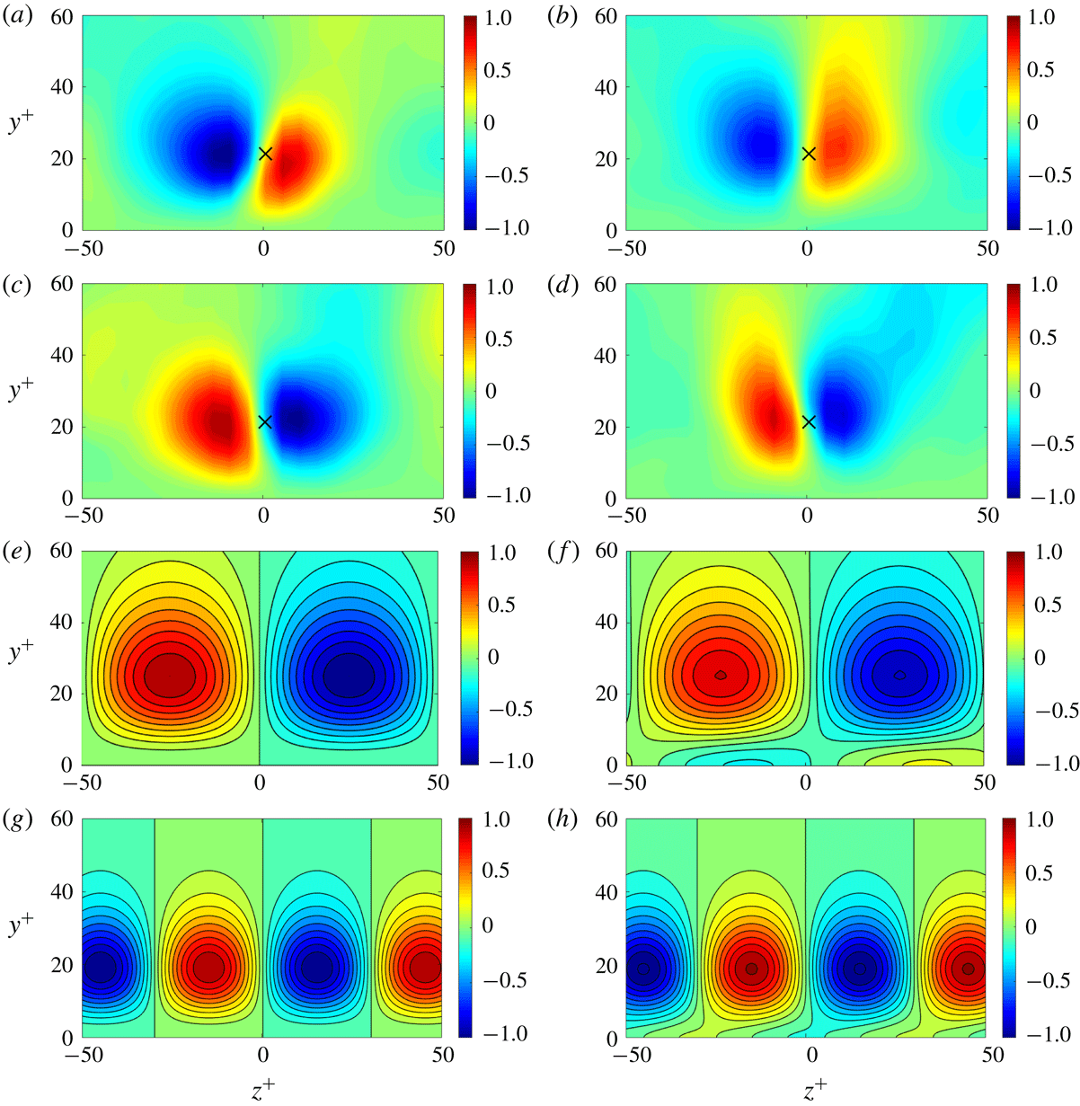
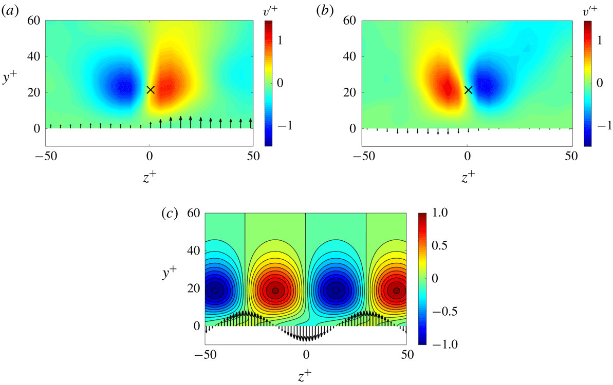
Figure 11(a–d) shows isocontours of the wall-normal velocity fluctuations obtained under conditional averaging, normalized by the maximum value in the uncontrolled case. Conditionally averaged flow fields for the uncontrolled and controlled CCW vortices are shown in panels (a) and (b), respectively. Similarly, flow fields for CW vortices in the uncontrolled and controlled case are shown in panels (c) and (d). The cross symbols in these four panels show vortex core locations. As expected, regions with negative (blue shading) and positive (red shading) wall-normal velocity are found to the left- and right-hand side of the crosses, respectively, for the CCW vortices, and vice versa for the CW vortices.
(a–d) Wall-normal velocity fluctuations
 ${v^{\prime }}^{+}$
associated with the quasi-streamwise vortices, obtained via conditional averaging: (a,c) uncontrolled flow fields; (b,d) flow fields for case STz-CA. CCW vortices (
 $\unicode[STIX]{x1D714}_{x}^{+}<0$
) are shown in (a,b) while CW vortices (
 $\unicode[STIX]{x1D714}_{x}^{+}>0$
) are shown in (c,d). (e,f) The structure of the wall-normal velocity field for resolvent modes resembling the NW cycle in regions with
 $\unicode[STIX]{x1D714}_{x}^{+}>0$
. (g,h) Resolvent mode structure for smaller modes with
 $(\unicode[STIX]{x1D706}_{x}^{+},\unicode[STIX]{x1D706}_{z}^{+},c^{+})=(300,60,10)$
. The uncontrolled mode structures are shown in (e,g) while the controlled mode structures are shown in (f,h).

A comparison of the controlled (figure 11
b,d) and uncontrolled (figure 11
a,c) flow fields shows that, for both CCW and CW vortices, case STz-CA leads to an observable reduction of vertical velocity fluctuations. The maximum value of
 $|v^{\prime }|^{+}$
for case STz is
 $1.1$
for CCW vortices, which is 25 % smaller than that in the uncontrolled case,
 $|v_{0,max}^{\prime }|^{+}=1.5$
. Similarly, the maximum value for CW vortices shows a roughly 10 % decrease from the uncontrolled case,
 $|v_{0,max}^{\prime }|^{+}=1.3$
, to the controlled case,
 $|v_{c,max}^{\prime }|^{+}=1.2$
. These conditionally sampled results indicate that the sweeps and ejections associated with the NW turbulence (i.e. the downward (
 $v^{\prime }<0$
) and upward (
 $v^{\prime }>0$
) flows induced by near-wall vortices) are weakened by control, and confirm that the newly proposed control laws are able to successfully suppress both QSVs and streaks. Suppression of these structures associated with the dynamically important NW cycle is essential to reducing turbulent skin friction at the relatively low Reynolds numbers tested here in DNS.
Figure 11(e,f) shows the predicted wall-normal velocity variation for uncontrolled and controlled resolvent modes resembling the NW cycle, i.e. modes with
 $(\unicode[STIX]{x1D706}_{x}^{+},\unicode[STIX]{x1D706}_{z}^{+},c^{+})\approx (10^{3},10^{2},10)$
. Similarly, figure 11(g,h) shows the velocity structure for smaller resolvent modes with length and velocity scales corresponding to the QSVs observed in near-wall turbulence,
 $(\unicode[STIX]{x1D706}_{x}^{+},\unicode[STIX]{x1D706}_{z}^{+},c^{+})\approx (300,60,10)$
. The typical streamwise length and diameter of these QSVs are known to be
 $l_{x}^{+}=150$
and
 $d^{+}=30$
, respectively, consistent with the conditionally averaged structures shown in figure 11(a–d). Note that the plotted velocity structure includes contributions from both oblique modes (with
 $k_{z}>0$
and
 $k_{z}<0$
) and is scaled with the predicted singular value. In other words, the plots show isocontours of
 $\unicode[STIX]{x1D70E}_{\boldsymbol{k}}v_{\boldsymbol{k}}$
, normalized by the maximum value in the uncontrolled case. Further, since resolvent modes are periodic structures, we focus on a
 $y$
–
 $z$
snapshot corresponding to
 $\unicode[STIX]{x1D714}_{x}^{+}>0$
and maximum wall-normal velocity. To observe regions with
 $\unicode[STIX]{x1D714}_{x}^{+}<0$
, the snapshot can simply be shifted by
 $\pm \unicode[STIX]{x1D706}_{z}^{+}/2$
in the spanwise direction.
The predicted resolvent mode structures are broadly consistent with the conditionally averaged flow fields obtained from DNS. Similar to the results shown in figure 11(c,d), the intensity of the vertical velocity fluctuations associated with the resolvent modes resembling the NW cycle is weakened under control (see figure 11
e,f). More quantitatively, the maximum value of
 $|\unicode[STIX]{x1D70E}_{\boldsymbol{k}}v_{\boldsymbol{k}}|$
decreases by 18 % from the uncontrolled case,
 $|\unicode[STIX]{x1D70E}_{\boldsymbol{k},0}v_{\boldsymbol{k},0}|_{max}=3.8$
, to case STz,
 $|\unicode[STIX]{x1D70E}_{\boldsymbol{k},c}v_{\boldsymbol{k},c}|_{max}=3.1$
, which is in good agreement with the reduction rate for conditionally averaged
 $|v_{max}^{\prime }|$
(figure 11
a–d). Further, the resolvent mode structure for the controlled case shows a slight tilt and a phase shift in the spanwise direction. This can be attributed to the spanwise asymmetry in the newly proposed control laws. As discussed in § 3.2, resolvent analysis predicts that case STz leads to greater suppression for NW-type resolvent modes with
 $k_{z}>0$
compared to modes with
 $k_{z}<0$
. This creates the spanwise tilt observed in figure 11(f,h). Case STz leads to similar structural changes for CCW vortices as well, though the predicted resolvent mode structures are not shown here.
Finally, note that the control input (blowing and suction) is phase-shifted relative to the wall-normal velocity field further away from the wall. As is evident in figure 11(f,h), case STz applies suction (blue shading) below the core of CW vortices, between the alternating regions of positive (red shading) and negative (blue shading) wall-normal velocity found further from the wall. Similarly, blowing is applied below the core of CCW vortices. We provide a physical explanation for this effect in the following section.
4.2 Physical interpretation of new control laws
The results presented thus far show that case STz is able to successfully suppress the streaks and QSVs associated with the NW cycle and generates skin friction reduction. However, the physical interpretation of the newly proposed laws – both case STz and case STrz – has not yet been clarified. In this section, we evaluate how the change in control law coefficient from
 $k_{x}/K$
for case ST to
 $\pm k_{z}/K$
for cases STz and STrz physically gives rise to the effects observed in DNS.
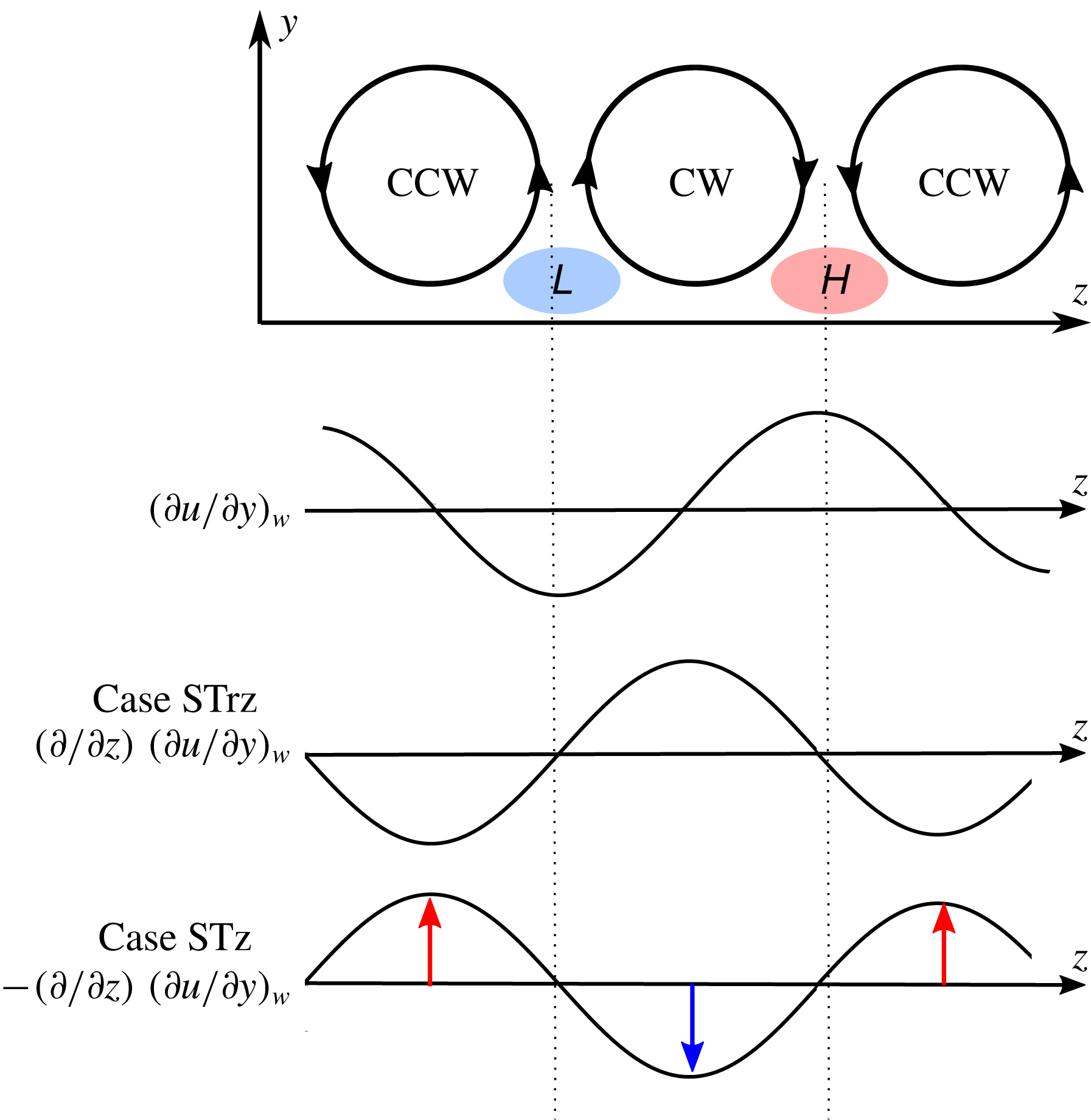
Schematic representation showing anticlockwise (CCW) and clockwise (CW) near-wall vortices, the resulting regions of high (red, H) and low (blue, L) streamwise wall shear stress, and the blowing or suction generated under case STrz and case STz.

Under an inverse Fourier transform, the
 $-\text{i}k_{z}$
prefactor in (3.6) changes to a partial derivative in the spanwise direction,
 $-\unicode[STIX]{x2202}/\unicode[STIX]{x2202}z$
. Thus, in physical space, case STz generates blowing and suction at the wall that is proportional to the first-order spanwise partial derivative of the streamwise wall shear stress,
 $\unicode[STIX]{x1D719}\propto -(\unicode[STIX]{x2202}^{2}u/\unicode[STIX]{x2202}y\unicode[STIX]{x2202}z)$
. Similarly, for case STrz, the following proportionality holds:
 $\unicode[STIX]{x1D719}\propto (\unicode[STIX]{x2202}^{2}u/\unicode[STIX]{x2202}y\unicode[STIX]{x2202}z)$
.
Figure 12 shows a schematic representation of the near-wall QSVs, the resulting wall shear stress, and the blowing or suction generated under cases STrz and STz. For CCW and CW vortices that are (statistically) aligned alternately in the spanwise direction, high- and low-speed streaks are expected in regions of downwelling (H) and upwelling (L), respectively. This induces alternating regions of high and low streamwise wall shear stress. Consideration of the spanwise partial derivative of this shear stress signal shows that case STz generates blowing under CCW vortices and suction under CW vortices. The opposite is true for case STrz: blowing is generated under CW vortices and suction is generated under CCW vortices.
To examine whether the physical interpretation of the control laws shown in figure 12 is also observed in DNS, we consider the relationship between the control input and vortex structure under conditional averaging. Figures 13(a) and 13(b) show the spanwise distribution of the conditionally averaged control input,
 $\unicode[STIX]{x1D719}^{+}$
, in case STz-CA for the CCW and CW vortices shown in figures 11(b) and 11(d), respectively. Note that the blowing-and-suction vectors are magnified
 $50\times$
(in terms of viscous units) for clarity. Figure 13(a) confirms that blowing is generated below the core of CCW vortices, and figure 13(b) confirms that suction is applied below the core of CW vortices. Further, figure 13(c) shows the wall-normal velocity fluctuations and control inputs for resolvent modes with
 $(\unicode[STIX]{x1D706}_{x}^{+},\unicode[STIX]{x1D706}_{z}^{+},c^{+})=(300,60,10)$
under case STz. The predicted inputs are in good agreement with the theoretical profile shown in figure 12; case STz applies blowing to CCW vortices and suction to CW vortices.
(a,b) Conditionally averaged wall-normal velocity fields (shading) for case STz-CA, along with the blowing and suction applied at the walls (black arrows): (a) CCW vortices and (b) CW vortices. Note that the blowing-and-suction vectors are magnified by a factor of 50 in viscous units. (c) Wall-normal velocity structure (shading) and predicted control input (arrows) for resolvent modes with
 $(\unicode[STIX]{x1D706}_{x}^{+},\unicode[STIX]{x1D706}_{z}^{+},c^{+})=(300,60,10)$
.

Wall-normal profiles of
 $\unicode[STIX]{x1D714}_{x,rms}^{+}$
. Results for case STz-CA are shown in (a), and results for case STrz-CA are shown in (b). The dashed lines and crosses represent the uncontrolled case, while the solid line and circles represent controlled cases. Black lines represent the total streamwise vorticity. Red lines consider only the positive component of vorticity,
 $\unicode[STIX]{x1D714}_{x}^{+}>0$
, corresponding to CW vortices, while blue markers only consider the negative component corresponding to CCW vortices.

To test whether this difference in actuation profiles for CW and CCW vortices generates differing statistics for positive and negative streamwise vorticity fluctuations, we consider the wall-normal profiles of r.m.s. vorticity,
 $\unicode[STIX]{x1D714}_{x,rms}^{+}$
, obtained in DNS. Figure 14 shows r.m.s. vorticity profiles for the uncontrolled case as well as both controlled cases, and further distinguishes between contributions from positive and negative vorticity fluctuations.
For the uncontrolled case, the total value of
 $\unicode[STIX]{x1D714}_{x,rms}^{+}$
(black dotted lines) shows good agreement with previously reported results (Moser et al.
Reference Moser, Kim and Mansour1999). As expected, the contributions from positive vorticity fluctuations (red dotted lines) and negative vorticity fluctuations (blue crosses) are identical. When control is applied, for both case STz and case STrz there is a substantial reduction in the total vorticity intensity (black solid lines) as well as contributions from positive (red solid lines) and negative (blue circles) vorticity fluctuations. Interestingly, there is no clear distinction between how these control laws affect positive or negative streamwise vorticity fluctuations. In other words, the fact that blowing is applied to CCW vortices and suction is applied to CW vortices for case STz (vice versa for case STrz) does not yield differing control effects on these structures; both CW and CCW streamwise vortices are suppressed equally due to control.
From the perspective of resolvent analysis, the above observations are not too surprising because each wavenumber–frequency combination is associated with alternating regions of positive and negative streamwise vorticity. Hence, any predicted mode suppression applies equally to both CW and CCW vortices. Moreover, given the spanwise homogeneity, turbulent channel flow does not have an inherent preference between oblique modes with
 $k_{z}>0$
or
 $k_{z}<0$
. As such, the statistical effect of cases STz and STrz is identical when contributions from modes with
 $k_{z}>0$
and modes with
 $k_{z}<0$
are taken together.
Schematic representation of streaks, QSVs, wall-normal velocity fluctuations, and blowing or suction generated under case STz, considering only modes with
 $k_{z}>0$
(a) and modes with
 $k_{z}<0$
(b). Note that contours show near-wall streaks,
 $u^{\prime }$
, which is different from the colour scheme employed in figure 7. Sinusoidal profiles below the shaded contours show the streamwise distributions of the wall-normal velocity fluctuations
 $v^{\prime }$
and the control input at the spanwise location corresponding to the white dashed line.

However, the physical interpretation of cases STz and STrz shown schematically in figure 12 does provide a potential explanation for why the effectiveness of these newly proposed control laws is asymmetric with respect to the sign of
 $k_{z}$
. As discussed in the previous sections, case STz is predicted to be more effective at suppressing NW-type resolvent modes with
 $k_{z}>0$
compared to those with
 $k_{z}<0$
. Figure 15 shows a schematic representation of the flow field and control input generated under case STz considering modes with either
 $k_{z}>0$
or
 $k_{z}<0$
. The shaded contours in this schematic represent the location of streaks (i.e. contours of near-wall
 $u^{\prime }$
), normalized by the maximum value. The streamwise distributions of the wall-normal velocity fluctuations and the control input at the spanwise location corresponding to the white dashed line are shown below the shaded contour plots. Note that
 $v^{\prime }>0$
where
 $u^{\prime }<0$
, and vice versa. This schematic representation in the
 $x$
–
 $z$
plane indicates that, for oblique modes with
 $k_{z}>0$
, the control input under case STz leads the wall-normal velocity field associated with the propagating flow structure (figure 15
a). In contrast, for oblique modes with
 $k_{z}<0$
the control input lags the wall-normal velocity field (figure 15
b). From a dynamic point of view, a control input that leads the velocity field may yield more effective suppression.
Several previous studies have evaluated the effect of phase on the efficacy of feedback flow control. Luhar et al. (Reference Luhar, Sharma and McKeon2014) investigated the effect of phase-shifted opposition control using resolvent analysis, showing that phase optimization could yield more significant drag reduction compared to the original opposition control. Note that introducing a phase shift within the (Fourier) resolvent mode framework is equivalent to varying sensor position relative to the actuator or introducing a time delay between the sensor and actuator. Similarly, Lee (Reference Lee2015) reported that using an upstream sensor improved the performance of opposition control. The use of an upstream sensor together with a time delay was also evaluated by Lee (Reference Lee2015). These previous efforts reinforce the present argument that phase difference play an important role in determining control efficacy.
5 Conclusions
Guided by previous resolvent-based predictions (Nakashima et al. Reference Nakashima, Fukagata and Luhar2017), in this study we reassessed suboptimal control performance via DNS, focusing on control over selective regions of spectral space. In addition, we proposed new feedback control laws for skin friction reduction that only require streamwise wall shear stress information.
In the original form proposed by Lee et al. (Reference Lee, Kim and Choi1998), suboptimal control based on the streamwise wall shear stress (case ST) generates an increase in drag. Resolvent analysis, pursued by Nakashima et al. (Reference Nakashima, Fukagata and Luhar2017), suggests that this increase in drag may be attributed to mixed control performance across spectral space, whereby structures with long streamwise wavelengths are suppressed by control while structures with shorter wavelengths are further amplified. Motivated by these resolvent-based predictions, we employed DNS to evaluate drag reduction with control applied only for large scales (case ST-CL). Contradicting resolvent-based predictions, DNS did not show a substantial change in drag even with this spectrally limited control. To identify the reason for this discrepancy, we calculated the blowing-and-suction amplitude (
 $\unicode[STIX]{x1D6FC}$
) imposed in the DNS. This a posteriori analysis revealed that the value of
 $\unicode[STIX]{x1D6FC}$
imposed in DNS was much smaller than the value used by Nakashima et al. (Reference Nakashima, Fukagata and Luhar2017), which was estimated assuming that the near-wall cycle is dominant. Thus, the lack of efficacy for case ST-CL can be attributed to low actuation amplitude. Even in additional DNS with increased blowing-and-suction amplitudes (
 $\unicode[STIX]{x1D719}_{rms}^{+}=0.5$
and
 $1$
),
 $\unicode[STIX]{x1D6FC}$
was still much smaller than that assumed by Nakashima et al. (Reference Nakashima, Fukagata and Luhar2017) and drag reduction could not be achieved.
Following this analysis, new control laws (cases STz and STrz) were developed and tested using a combination of resolvent analysis and DNS. The original control law proposed by Lee et al. (Reference Lee, Kim and Choi1998) includes the streamwise wavenumber,
 $k_{x}$
, as a multiplicative factor in determining the control amplitude. The new laws proposed here replace the streamwise wavenumber with the spanwise wavenumber,
 $\pm k_{z}$
, to increase the magnitude of blowing and suction applied to structures with long streamwise wavelengths (i.e. small
 $k_{x}$
). Resolvent analysis suggests that these new control laws suppress large-scale flow structures with wavelengths similar to the NW cycle, but have little effect on small-scale flow structures.
Note that these newly proposed control laws also introduce a spanwise asymmetry that depends on whether
 $+k_{z}$
or
 $-k_{z}$
is used to determine actuation magnitude. In other words, the new control laws have differing effects on oblique structures with wavenumber combinations
 $(k_{x},k_{z})$
and (
 $k_{x},-k_{z}$
). Case STz has the same effect on modes with
 $k_{z}>0$
as case STrz does on modes with
 $k_{z}<0$
, and vice versa. This oblique asymmetry is evident in resolvent-based predictions for mode suppression across spectral space, as well as the flow fields obtained in DNS. Statistically, structures with positive and negative
 $k_{z}$
are expected to be equally prevalent in turbulent channel flow, and so the new control laws are expected to show the same integrated effect on drag reduction. DNS results are again consistent with resolvent-based predictions in this regard, i.e. cases STz and STrz yield identical integrated effects.
DNS with the newly proposed laws shows approximately 10 % drag reduction. These results are broadly consistent with resolvent-based predictions for mode suppression. Further, the global statistics obtained here (e.g. profiles of mean velocity and r.m.s. velocity fluctuations) show characteristics similar to those reported in previous DNS studies of successful feedback flow control (Choi et al. Reference Choi, Moin and Kim1994; Lee et al. Reference Lee, Kim and Choi1998). The mean streamwise velocity decreases slightly in the viscous sublayer and buffer layer, and r.m.s. values for all components of the fluctuating velocity are reduced across the channel.
We also examined 2D premultiplied co-spectra for cases ST and STz. Unlike case ST, the newly proposed case STz successfully suppressed co-spectra for all components of velocity,
 $E_{uu}$
,
 $E_{vv}$
and
 $E_{ww}$
. Although resolvent analysis does not predict mode suppression for small-scale structures with case STz, DNS shows a significant decrease in spectral strength for both large and small scales. We attribute this discrepancy to the broadband forcing assumption employed for resolvent analysis, whereby the nonlinear term is considered to be of uniform strength across spectral space. In reality, suppression of large-scale structures would also lead to a decrease in nonlinear energy transfer to small scales.
Finally, we employed conditional sampling and further theoretical analysis to provide insight into the physical mechanisms leading to drag reduction under cases STz and STrz. This effort revealed that case STz effectively suppresses the sweeps and ejections associated with the NW cycle (i.e. the downward (
 $v^{\prime }<0$
) and upward (
 $v^{\prime }>0$
) flows induced by near-wall vortices), and that this new control law applies blowing to anticlockwise (CCW) quasi-streamwise vortices and suction under clockwise (CW) vortices. On the other hand, case STrz applies suction to CCW vortices and blowing to CW vortices. Despite this difference, profiles of
 $\unicode[STIX]{x1D714}_{x,rms}^{+}$
considering only
 $\unicode[STIX]{x1D714}_{x}^{+}>0$
(CW vortices) or
 $\unicode[STIX]{x1D714}_{x}^{+}<0$
(CCW vortices) show no difference in the extent to which CW and CCW vortices are suppressed by either case STz or case STrz. In other words, even though these new control laws apply opposing inputs to CCW and CW vortices, there is no observable difference in how these vortices are affected by control. This result is natural in the context of travelling-wave resolvent modes, which comprise alternating regions of
 $\unicode[STIX]{x1D714}_{x}<0$
and
 $\unicode[STIX]{x1D714}_{x}>0$
. If control successfully suppresses a given resolvent mode, then both CW and CCW vortices are suppressed, regardless of the actual actuation profile.
Even though this difference in actuation for CW and CCW vortices does not lead to statistical differences in net effect under cases STz and STrz, it does provide physical insight into why these control laws lead to contrasting effects on oblique modes with
 $k_{z}>0$
and
 $k_{z}<0$
. Specifically, under case STz the control input leads the flow field for modes with
 $k_{z}>0$
and lags the flow field for modes with
 $k_{z}<0$
. Resolvent analysis shows that, in general, case STz yields larger suppression for NW modes with
 $k_{z}>0$
compared to modes with
 $k_{z}<0$
. The converse is true for case STrz, i.e. the actuation leads the flow field for modes with
 $k_{z}<0$
, and yields greater mode suppression. Together, these observations indicate that control is more effective when the actuation leads the flow field.
Acknowledgements
A.K., S.N. and K.F. are grateful to Drs S. Obi and K. Ando (Keio University) for fruitful discussions. This work was supported through JSPS KAKENHI grant numbers 25420129 and 18H03758 by the Japan Society for the Promotion of Science (JSPS). This material is based upon work supported by the Air Force Office of Scientific Research under award number FA9550-17-1-0142 (M.L.).