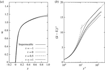
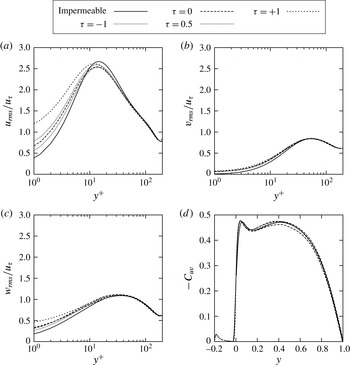
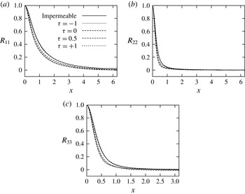
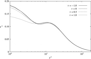
1. Introduction
There are two main motivations for this study: to further improve the understanding of the effects of porous materials on engineering and natural flows, and to gain insight into the design of novel porous materials. There are, in fact, many engineering applications involving fluid flows over or through porous materials that will benefit from a better understanding of the role played by these materials, such as extraction of oil from ground reservoirs, management of water ground basins and filtration of pollutants through aquifers, transpiration cooling, in which the porosity is used to enhance the heat exchange capability of the material, and filtration processes used to separate solid particles from fluids. Examples in nature are flows through sedimentary rocks, such as sandstones, conglomerates and shales, and water flows over seabeds and riverbeds. Porous media also play a crucial role in many biological processes involving fluid and mass transfer at the walls of many organic tissues, such as blood vessels, lungs and kidneys. The ability to design porous materials with specific properties (e.g., porosity, permeability, momentum transfer at the interface, etc.) could lead to novel developments in several fields spanning from aerodynamics to biology, and from chemistry to medicine.
The main properties characterizing a porous material are porosity and permeability. These are obviously average properties measured on samples of porous materials large with respect to the characteristic pore size. Porosity (or void fraction),
 ${\it\varepsilon}$
, is a dimensionless measure of the void spaces in a material. It is expressed as a fraction of the volume of voids over the total volume and its value varies between 0 and 1. Permeability,
 $K^{\ast }$
, with dimensions of length squared, is a measure of the ease with which a fluid flows through a porous medium (throughout this article, an asterisk denotes a dimensional quantity).
 $K^{\ast }=0$
if a medium is impermeable, i.e., if no fluid can flow through it, while it becomes infinite if a medium offers no resistance to a fluid flow. Typical values of porosity for porous materials made of packed particles are (see Macdonald et al.
Reference Macdonald, El-Sayed, Mow and Dullien1979)
 $0.366<{\it\varepsilon}<0.64$
for spherical glass beads packed in a ‘uniformly random’ manner,
 $0.367<{\it\varepsilon}<0.515$
for spherical marble mixtures, sand and gravel mixtures, and ground Blue Metal mixtures,
 $0.123<{\it\varepsilon}<0.378$
for a variety of consolidated media,
 $0.32<{\it\varepsilon}<0.59$
for a wide variety of cylindrical packings, and
 $0.682<{\it\varepsilon}<0.919$
for cylindrical fibres. Beavers & Joseph (Reference Beavers and Joseph1967) performed experiments with three types of foametals
 $0.78<{\it\varepsilon}<0.79$
and two types of aloxites
 $0.52<{\it\varepsilon}<0.58$
.
The first empirical law governing Stokes flow through porous media was derived by Darcy (see Lage Reference Lage1998) in 1856. More than a century later, Beavers & Joseph (Reference Beavers and Joseph1967) presented the first interface (jump) condition coupling a porous flow governed by Darcy’s law with an adjacent fully developed laminar channel flow. This condition was further developed, with different degrees of success, by Neale & Nader (Reference Neale and Nader1974), Vafai & Thiyagaraja (Reference Vafai and Thiyagaraja1987), Vafai & Kim (Reference Vafai and Kim1990) and Hahn, Je & Choi (Reference Hahn, Je and Choi2002), among others. General porous flow equations, the so-called volume-averaged Navier–Stokes equations (VANS), were derived by Whitaker (Reference Whitaker1996) by volume-averaging the Navier–Stokes (NS) equations. The VANS equations show some analogy with LES equations. Ochoa-Tapia & Whitaker (Reference Ochoa-Tapia and Whitaker1995a ) introduced a momentum-transfer condition, involving a shear stress jump at the porous/fluid interface, necessary to couple the VANS equations (governing the flow within the porous material) to the NS equations (governing the free flowing fluid). Over the years this condition was further developed by Alazmi & Vafai (Reference Alazmi and Vafai2001), Goyeau et al. (Reference Goyeau, Lhuillier, Gobin and Velarde2003), Chandesris & Jamet (Reference Chandesris and Jamet2006), Valdés-Parada, Goyeau & Ochoa-Tapia (Reference Valdés-Parada, Goyeau and Ochoa-Tapia2007), Chandesris & Jamet (Reference Chandesris and Jamet2007, Reference Chandesris and Jamet2009) and Valdés-Parada et al. (Reference Valdés-Parada, Aguilar-Madera, Ochoa-Tapia and Goyeay2013). Recently, Minale (Reference Minale2014a ,Reference Minale b ) rederived the momentum-transfer condition from physical principles using the volume-averaging approach introduced by Ochoa-Tapia & Whitaker (Reference Ochoa-Tapia and Whitaker1995a ). Minale computed the stress transferred from the free flowing fluid to both the fluid within the porous medium and to the porous matrix, and then imposed a zero-stress jump at the interface, effectively preserving the total stress at it. Although physically sound, the boundary condition obtained by Minale in practice produces results similar to those obtained when using the condition derived by Ochoa-Tapia & Whitaker (Reference Ochoa-Tapia and Whitaker1995a ) and Valdés-Parada et al. (Reference Valdés-Parada, Aguilar-Madera, Ochoa-Tapia and Goyeay2013).
The main effects of porous materials on adjacent fluid flows are the destabilization of laminar flows and the enhancement of the Reynolds-shear stresses, with a consequent increase in skin-friction drag in turbulent flows. The first results showing the destabilizing effects of wall permeability were obtained experimentally by Beavers, Sparrow & Magnuson (Reference Beavers, Sparrow and Magnuson1970). Sparrow et al. (Reference Sparrow, Beavers, Chen and Lloyd1973) experimentally determined a few critical Reynolds numbers in a channel with one porous wall, and performed a two-dimensional temporal linear stability analysis using Darcy’s law with the interface condition introduced by Beavers & Joseph (Reference Beavers and Joseph1967). Several years later, Tilton & Cortelezzi (Reference Tilton and Cortelezzi2006, Reference Tilton and Cortelezzi2008) performed a three-dimensional temporal linear stability analysis of a laminar flow in a channel with one or two homogeneous, isotropic, porous walls by modelling the flow in the porous walls using the VANS equations with the interface conditions of Ochoa-Tapia & Whitaker (Reference Ochoa-Tapia and Whitaker1995a ). They reported that wall permeability can drastically decrease the stability of fully developed laminar channel flows. Recently, Tilton & Cortelezzi (Reference Tilton and Cortelezzi2015) performed a spatial linear stability analysis of the asymptotic suction boundary layer developing over a rigid, homogeneous, isotropic, porous layer of small permeability, in which inertial effects may be neglected. The porous layer is bounded above by a semi-infinite region in which a boundary layer is driven by a constant free-stream velocity. The wall suction is created by applying a suction pressure to a semi-infinite region below the porous layer. Their stability analysis takes account of the full coupling between the flow fields in the boundary-layer and suction regions, governed by the NS equations, and the flow in the porous layer, governed by the VANS equations with the interface conditions of Ochoa-Tapia & Whitaker (Reference Ochoa-Tapia and Whitaker1995a ). Tilton & Cortelezzi (Reference Tilton and Cortelezzi2015) reported that small amounts of wall permeability destabilize the Tollmien–Schlichting wave and cause a substantial broadening of the unstable region. As a result, the stabilization of boundary layers by wall suction is substantially less effective and more expensive than what is predicted by classical boundary-layer theory.
There is also a scarcity of literature regarding the effects of permeability on turbulent flows. Early experiments by Lovera & Kennedy (Reference Lovera and Kennedy1969) on alluvial streams over flat sand beds showed increasing skin-friction coefficient with increasing Reynolds number. Ruff & Gelhar (Reference Ruff and Gelhar1972) investigated turbulent flows in a pipe lined with highly porous foam. They recognized the importance of the exchange of momentum across the porous/fluid interface and reported higher skin friction for porous walls than for solid walls. Experimentally, Zagni & Smith (Reference Zagni and Smith1976) reported higher skin friction for open-channel flows over permeable beds of packed spheres than over impermeable walls, and attributed the increase to the additional energy dissipation caused by the exchange of momentum across the fluid–porous interface. Kong & Schetz (Reference Kong and Schetz1982) measured an increase in skin friction in boundary layers over porous walls made of sintered metals, bonded screen sheets and perforated titanium sheets. In wind-tunnel experiments of boundary layer flows over a bed of grains, Zippe & Graf (Reference Zippe and Graf1983) reported a rise in skin friction with respect to impermeable rough walls. Shimizu, Tsujimoto & Nakagawa (Reference Shimizu, Tsujimoto and Nakagawa1990) investigated the flow induced in the transition layer, just below the porous/fluid interface, and concluded that permeability enhances momentum flux and Reynolds stresses near the interface. Hahn et al. (Reference Hahn, Je and Choi2002) performed a DNS of a turbulent plane channel flow by modelling the presence of permeable walls with boundary conditions similar to those introduced by Beavers & Joseph (Reference Beavers and Joseph1967), i.e. finite tangential (slip) velocity and zero normal velocity. They reported ‘significant skin-friction reductions’ at the permeable walls. This result conflicts with the experimental evidence and is presumably due to the enforcement of a zero normal velocity at the porous/fluid interface, a boundary condition that inhibits the correct exchange of momentum across the interface (e.g. Ruff & Gelhar Reference Ruff and Gelhar1972). It is also interesting to note that Perot & Moin (Reference Perot and Moin1995) performed a DNS of a turbulent plane channel flow with infinite permeability and no-slip boundary conditions in order to remove the wall-blocking mechanism and study the contribution of splashes on wall turbulence.
In order to describe accurately the mass and momentum transfer between a fluid-saturated porous layer and a turbulent flow, one could, in principle, perform a DNS by solving the NS equations over the entire domain and enforcing the no-slip and no-penetration conditions on the highly convoluted surface representing the boundary of the porous material. In practice, however, this approach is hard to implement because the boundary of a porous material has, in general, an extremely complex geometry that, often, is not known in full details. Therefore, this approach has been used only in cases in which the porous medium is highly idealized and has a simple geometry. Zhang & Prosperetti (Reference Zhang and Prosperetti2009) and Liu & Prosperetti (Reference Liu and Prosperetti2011) modelled the porous walls of a channel using disjointed cylinders and spheres in a simple cubic arrangement and studied the lift, drag and torque generated on the cylindrical and spherical particles by a fully developed laminar flow. Breugem & Boersma (Reference Breugem and Boersma2005) and Chandesris et al. (Reference Chandesris, D’Hueppe, Mathieu, Jamet and Goyeau2013) used a three-dimensional Cartesian grid of disjointed cubes. The former investigated the effect of porous walls on the statistics of a fully turbulent channel flow, the latter investigated the effects on turbulent heat transfer.
Breugem & Boersma (Reference Breugem and Boersma2005) used two approaches to model the flow through a porous material and characterize the effects of permeability on fully turbulent channel flows delimited by one porous wall and one solid wall. In the first approach, they performed a DNS of a turbulent channel flow over a three-dimensional Cartesian grid of disjointed cubes mimicking a permeable wall with
 ${\it\varepsilon}=0.875$
, and solved the NS equations over the entire domain. In the second approach, they performed a DNS of the channel flow by solving the NS equations in the fluid region and the VANS equations in the porous layers. In particular, they used the model developed by Irmay (Reference Irmay1965) to express permeability in terms of porosity, the Burke–Plummer equation to express the Forchheimer tensor in terms of porosity and a fifth-order polynomial function to model the variation of porosity in the thin porous region adjacent to the porous/fluid interface, known as the transition layer. This comparison is particularly meaningful because the VANS equations were obtained by volume-averaging the NS equations over the Cartesian grid of disjointed cubes used in the DNS simulations. The main conclusion of the study by Breugem & Boersma (Reference Breugem and Boersma2005) was that ‘the approach based on the VANS equations is capable of an accurate simulation of the turbulent flow over and through a permeable wall, even quantitatively’.
One year later, Breugem, Boersma & Uittenbogaard (Reference Breugem, Boersma and Uittenbogaard2006) leveraged the work by Breugem & Boersma (Reference Breugem and Boersma2005) to study the influence of a highly permeable porous wall, made by a packed bed of particles, on turbulent channel flows. To isolate the effect of wall permeability from that of wall roughness, they considered highly porous packed beds made of particles of small mean diameter, two apparently conflicting requirements leading to beds of disjointed particles. Because of these assumptions, the fluid quickly flows through the porous medium and the drag force cannot be neglected. The authors modelled it by means of the Ergun equation (Bird, Stewart & Lightfoot Reference Bird, Stewart and Lightfoot2002) in combination with a fifth-order variable-porosity model, thus ensuring the continuity of both porosity and drag force over the interface region. In this approach, the permeability and the Forchheimer tensors (responsible for the drag force) can be written in terms of porosity and mean particle diameter. The authors presented the results of four simulations for values of porosity equal to 0, 0.6, 0.8 and 0.95, and classified the permeable walls as highly permeable (near which viscous effects are of minor importance,
 $Re_{K}\equiv \sqrt{K^{\ast }}u_{{\it\tau}}^{\ast }/{\it\nu}^{\ast }=9.35$
, where
 $u_{{\it\tau}}^{\ast }$
is the friction velocity and
 ${\it\nu}^{\ast }$
is the kinematic viscosity) in the case
 ${\it\varepsilon}=0.95$
, partially permeable (
 $Re_{K}=1.06$
) in the case
 ${\it\varepsilon}=0.80$
and effectively impermeable (near which viscous diffusion of mean kinetic energy is counterbalanced by viscous dissipation,
 $Re_{K}=0.31$
) in the case
 ${\it\varepsilon}=0.60$
. Their results showed that the structure and dynamics of turbulence above a highly permeable wall, where there are no low- and high-speed streaks and quasi-streamwise vortices, are very different from those of a turbulent flow over an effectively impermeable wall. Near a highly permeable wall, turbulence is dominated by relatively large vortical structures that favour the exchange of momentum between the top layer of the porous medium, the transition layer, and the channel, and induce a strong increase in the Reynolds-shear stresses and, consequently, a strong increase in the skin friction compared to an impermeable wall.
Suga et al. (Reference Suga, Matsumura, Ashitaka, Tominaga and Kaneda2010) studied experimentally the effects of wall permeability on a turbulent flow in a channel with a porous wall. They considered three types of foamed ceramic materials whose porosity was almost the same (
 ${\it\epsilon}\approx 0.8$
), but whose permeabilities varied by a factor of approximately four,
 $K^{\ast }=0.020,0.033$
and
 $0.087~\text{mm}^{2}$
. They observed that the slip velocity of a flow over a permeable wall increases drastically in the range of Reynolds numbers where the flow transitions from laminar to turbulent, and that transition to turbulence appears at progressively lower Reynolds numbers as permeability increases, consistent with the results of linear stability analysis (Tilton & Cortelezzi Reference Tilton and Cortelezzi2006, Reference Tilton and Cortelezzi2008). The turbulence statistics of the velocity fluctuations showed that the wall-normal component increases as the wall permeability and/or the Reynolds number increases. The authors concluded that permeability weakens the blocking effects of a porous wall on the vortex motion, therefore contributing to an increase of the wall-shear stress, a conclusion consistent with similar observations put forward, among others, by Hahn et al. (Reference Hahn, Je and Choi2002). Suga et al. (Reference Suga, Matsumura, Ashitaka, Tominaga and Kaneda2010) also performed a numerical simulation of the same turbulent flow using the analytic wall function at the porous/fluid interface and found their results in good agreement with their experimental results and the results by Breugem et al. (Reference Breugem, Boersma and Uittenbogaard2006).
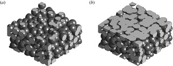
Effect of surface machining on the same numerically generated porous sample: between-particles cut (a) and through-particles cut (b) yield highly different interfaces.

The flow at the interface and in the transition region within the porous layer depends, for a given porous material, mostly on the surface machining of the interface. Figure 1 shows that even using the same (numerically generated) porous sample and the same surface machining technique, a totally different interfacial geometry is obtained simply by cutting the porous material half of a particle diameter deeper. Obviously, the flow just above the interface and within the transition region for the two samples shown in figure 1 will be noticeably different. Therefore, in general, it is nearly impossible to introduce a variable-porosity model that is capable of fitting all possible interface geometries, even if the porous material used is exactly the same. On the contrary, we believe that making a choice for a variable-porosity model reduces the generality of the model to a particular porous material with a particular interface.
The complexity of modelling the flow at the porous/fluid interface and within the transition region becomes less severe for porous materials of small permeability and small mean particle size. In particular, for sufficiently low permeabilities, the fluid velocity at the interface is small; consequently the convective effects and the drag force experienced by the fluid become negligible, because the dense channel-like structures of the porous matrix impede motion between layers of fluid. In this case, the transition region (of the order of a few pore diameters thick) and roughness (of the order of one pore diameter high) can be assumed to have zero thickness, and porosity and permeability to have a constant value up to an interface that has a clearly defined position (Ochoa-Tapia & Whitaker Reference Ochoa-Tapia and Whitaker1995a
, Reference Ochoa-Tapia and Whitaker1998; Valdés-Parada et al.
Reference Valdés-Parada, Goyeau and Ochoa-Tapia2007; Valdés-Parada et al.
Reference Valdés-Parada, Aguilar-Madera, Ochoa-Tapia and Goyeay2013). As a consequence, porosity and permeability are effectively decoupled because they are assumed to be constant up to the porous/fluid interface. The zero-thickness assumption produces a jump in the shear stresses at the interface because, at the interface, the sphere over which the volume averaging is performed lies partly in the porous region and partly in the free fluid region (see figure 3). This jump in stress produces an additional boundary condition at the interface, where the magnitude of the jump is proportional to a dimensionless parameter
 ${\it\tau}$
, the momentum-transfer coefficient, which is of the order of one and can be both positive or negative (Ochoa-Tapia & Whitaker Reference Ochoa-Tapia and Whitaker1995a
; Valdés-Parada et al.
Reference Valdés-Parada, Goyeau and Ochoa-Tapia2007; Valdés-Parada et al.
Reference Valdés-Parada, Aguilar-Madera, Ochoa-Tapia and Goyeay2013). The parameter
 ${\it\tau}$
is decoupled from porosity and permeability. In a recent interpretation by Minale (Reference Minale2014a
,Reference Minale
b
), a negative
 ${\it\tau}$
quantifies the amount of stress transferred from the free fluid to the porous matrix, while a positive
 ${\it\tau}$
quantifies the amount of stress transferred from the porous matrix to the free fluid; when
 ${\it\tau}=0$
the stress carried by the free fluid is fully transferred to the fluid saturating the porous matrix. In this study we use the stress jump condition introduced by Ochoa-Tapia & Whitaker (Reference Ochoa-Tapia and Whitaker1995a
), to be consistent with the work of Tilton & Cortelezzi (Reference Tilton and Cortelezzi2006, Reference Tilton and Cortelezzi2008, Reference Tilton and Cortelezzi2015) that inspired the present study. Although the relationship between linear stability of channel flows and fully turbulent channel flows is not immediate, we will show that the assessment of the effects of the porous parameters made by Tilton & Cortelezzi (Reference Tilton and Cortelezzi2008) in their linear stability analysis of pressure-driven channel flows with porous walls is remarkably accurate for fully turbulent channel flows at low Reynolds numbers.
A porous wall of small permeability
 $K^{\ast }$
is often thought to behave as an effectively impermeable wall. It is true that, in the limit
 $K^{\ast }\rightarrow 0$
, a porous wall becomes impermeable and behaves as a solid wall. On the other hand, as has been shown by Tilton & Cortelezzi (Reference Tilton and Cortelezzi2006, Reference Tilton and Cortelezzi2008, Reference Tilton and Cortelezzi2015), very small amounts of permeability have major effects on the stability of fully developed laminar flows in channels with one or both porous walls, and even on asymptotic suction boundary layers. In particular, the critical Reynolds number is most sensitive to small permeabilities, where it experiences its sharpest drop. Hence, in this paper we focus on low-permeability porous materials. There are two main reasons for this choice. First, porous materials of small permeabilities are common in nature and in industrial applications and, therefore, it is of interest to characterize their effects on turbulent flows. Second, since porosity, permeability and momentum-transfer coefficient are decoupled in the model used in the present study, our results could provide insights for the design of novel porous materials which target specific engineering applications.
In this work we describe the development and implementation of a computer code for the DNS of turbulent channel flows bounded by porous walls. The numerical method, based upon a pseudo-spectral strategy, employs Fourier discretization in the homogeneous directions and compact finite differences in the wall-normal direction, and it is used both in the fluid region and within the porous walls. Within the former the full NS equations are solved, while within the latter the VANS equations are solved, neglecting the inertial terms. After validating the numerical method against linear stability theory, the fully turbulent case is addressed. A parametric study is performed by varying all the parameters defining the porous medium (permeability, porosity and thickness) in order to assess their effect on turbulence statistics. Furthermore, the effects of the transition layer and interface machining are accounted for by varying the parameter controlling the shear stress jump at the interface in order to mimic the unavoidable uncertainty related to the real interface. Although not the main focus of the present work, the effect of varying the channel flow bulk Reynolds number is also briefly discussed.
The paper is organized as follows: in § 2, we discuss the channel geometry, governing equations and interface conditions. We then present the numerical method used to perform the DNS. The code is then validated against results predicted by linear stability theory. In § 3, we describe in statistical terms the effects of the porous material on a fully developed turbulent flow in a baseline case where the porous medium has small permeability, and then discuss the effects of varying the parameters of the porous material. Finally, we present a concluding summary in § 4.
2. Problem definition and mathematical formulation
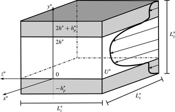
We consider the fully developed flow of an incompressible viscous fluid in a channel delimited by two identical, flat, rigid, homogeneous and isotropic, infinite porous layers sealed by impermeable walls, see figure 2. The upper and lower interfaces between the fluid and the porous material are located at
 $y^{\ast }=0$
and
 $y^{\ast }=2h^{\ast }$
, while the upper and lower impermeable walls are located at
 $y^{\ast }=-h_{p}^{\ast }$
and
 $y^{\ast }=2h^{\ast }+h_{p}^{\ast }$
, where
 $h^{\ast }$
is the half-height of the fluid region and
 $h_{p}^{\ast }$
is the height of the identical porous layers, respectively.
Sketch of the channel geometry. The interfaces between the channel region and the porous walls are located at
 $y^{\ast }=0$
and
 $y^{\ast }=2h^{\ast }$
; the porous walls have thickness
 $h_{p}^{\ast }$
, so that the two impermeable walls bounding the whole domain are at
 $y^{\ast }=-h_{p}^{\ast }$
and
 $y^{\ast }=2h^{\ast }+h_{p}^{\ast }$
.

The Reynolds number of the flow is defined as
 $$\begin{eqnarray}\mathit{Re}=\frac{U_{b}^{\ast }h^{\ast }}{{\it\nu}^{\ast }},\end{eqnarray}$$
where
 $h^{\ast }$
is the characteristic length scale and the characteristic velocity is the bulk velocity
 $U_{b}^{\ast }$
, defined as the average value of the mean velocity
 $\overline{u}^{\ast }(y^{\ast })$
computed across the whole domain, i.e.
 $$\begin{eqnarray}U_{b}^{\ast }=\frac{1}{2h^{\ast }}\int _{-h_{p}^{\ast }}^{2h^{\ast }+h_{p}^{\ast }}\overline{u}^{\ast }\,\text{d}y^{\ast }.\end{eqnarray}$$
Note that the integral spans over all three regions (fluid region and porous layers) while the weighting,
 $1/2h^{\ast }$
, accounts for the fluid region only. This choice, dictated by the fact that the mass flux in the porous layers is negligible in comparison to the total mass flux (especially at low permeabilities), facilitates the comparison between the flow in a channel with porous walls and the flow in a channel bounded by impermeable walls. In the next section we present the mathematical formulation of the problem made dimensionless by using
 $h^{\ast }$
,
 $U_{b}^{\ast }$
and
 $h^{\ast }/U_{b}^{\ast }$
as characteristic length, velocity and time, respectively.
2.1. Velocity–pressure formulation
The flow of an incompressible viscous fluid through the domain sketched in figure 2 is governed by the non-dimensional Navier–Stokes equations
 $$\begin{eqnarray}\displaystyle & \displaystyle \frac{\partial \boldsymbol{u}}{\partial t}+(\boldsymbol{u}\boldsymbol{\cdot }\boldsymbol{{\rm\nabla}})\boldsymbol{u}=-\boldsymbol{{\rm\nabla}}p+\frac{1}{\mathit{Re}}{\rm\nabla}^{2}\boldsymbol{u}, & \displaystyle\end{eqnarray}$$
 $$\begin{eqnarray}\displaystyle & \displaystyle \boldsymbol{{\rm\nabla}}\boldsymbol{\cdot }\boldsymbol{u}=0. & \displaystyle\end{eqnarray}$$
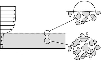
Sketch of a porous medium, with
 $\ell _{f}^{\ast }$
and
 $\ell _{s}^{\ast }$
the characteristic lengths of the pore and particle diameters of the pore-like structures.

However, it is nearly impossible to apply this model to a flow confined by porous layers because porous materials, in general, have very complex geometries and are characterized by a wide range of length scales. As exemplified in figure 3, such scales are bounded by the smallest scales
 $\ell _{f}^{\ast }$
(of the fluid phase) and
 $\ell _{s}^{\ast }$
(of the solid phase), related to the characteristic pore and particle diameters of the pore-like structures, and the largest scale
 $L_{p}^{\ast }$
, which is the characteristic thickness of the porous layer. To overcome these difficulties, Whitaker (Reference Whitaker1969, Reference Whitaker1986, Reference Whitaker1996) proposed to model only the large-scale behaviour of a flow in a porous medium by averaging the NS equations over a small sphere, of volume
 $V^{\ast }$
and radius
 $r^{\ast }$
. This averaging procedure, which is similar to the LES decomposition, results in the so-called volume-averaged Navier–Stokes (VANS) equations, and relies on the assumption that the length scales of the problem are well separated, i.e.,
 $\ell _{s}^{\ast }\sim \ell _{f}^{\ast }\ll r^{\ast }\ll L_{p}^{\ast }$
. Under this assumption, the volume-averaged quantities are smooth and free of small-scale fluctuations. In other words, the fluid-saturated porous medium is described as a continuum, so that fluid quantities, such as velocity or pressure, are defined at every point in space, regardless of their position within the fluid or solid phase.
The first step in the derivation of the VANS equations consists in choosing the appropriate averaging method. The superficial volume average
 $\langle {\it\phi}^{\ast }\rangle ^{s}$
, of a generic scalar quantity
 ${\it\phi}^{\ast }$
, is defined (Quintard & Whitaker Reference Quintard and Whitaker1994; Whitaker Reference Whitaker1996) as
 $$\begin{eqnarray}\langle {\it\phi}^{\ast }\rangle ^{s}=\frac{1}{V^{\ast }}\int _{V_{f}^{\ast }}{\it\phi}^{\ast }\,\text{d}V_{f}^{\ast },\end{eqnarray}$$
where
 $V_{f}^{\ast }<V^{\ast }$
is the volume of fluid contained within the averaging volume
 $V^{\ast }$
, while the intrinsic volume average is defined as
 $$\begin{eqnarray}\langle {\it\phi}^{\ast }\rangle ^{\,f}=\frac{1}{V_{f}^{\ast }}\int _{V_{f}^{\ast }}{\it\phi}^{\ast }\,\text{d}V_{f}^{\ast }.\end{eqnarray}$$
These two averages are related as follows
 $$\begin{eqnarray}\langle {\it\phi}^{\ast }\rangle ^{s}=\frac{V_{f}^{\ast }}{V^{\ast }}\langle {\it\phi}^{\ast }\rangle ^{\,f}={\it\varepsilon}\langle {\it\phi}^{\ast }\rangle ^{\,f},\end{eqnarray}$$
where
 ${\it\varepsilon}=V_{f}^{\ast }/V^{\ast }$
is the porosity, or the volume-fraction of fluid contained in
 $V^{\ast }$
, which is generally a function of the position in a heterogeneous porous medium.
The second step in the derivation of the VANS equations consists in defining a relationship between the volume average of a derivative of a scalar quantity and the derivative of the volume average of the same quantity, both for time and spatial derivatives. The general transport theorem (Whitaker Reference Whitaker1969), a generalized formulation of the Reynolds transport theorem, provides us with a relationship for the volume average of a time derivative, while the spatial averaging theorem (Slattery Reference Slattery1967; Whitaker Reference Whitaker1969) provides us with a relationship for the volume average of a spatial derivative.
Finally, assuming the porous material to be homogeneous and isotropic, i.e. porosity and permeability remain constant throughout the porous walls, and permeability to be sufficiently small to neglect inertial effects, the dimensionless VANS equations become linear because the drag term containing the Forchheimer tensor can be neglected with respect to the Darcy drag. In their linear stability study, Tilton & Cortelezzi (Reference Tilton and Cortelezzi2008) verified that this linearity assumption amounts to considering the longitudinal velocity at the porous/fluid interface to be lower than approximately 5 % of the centreline velocity of the channel. Since the focus of the present work are the effects of porous materials of small permeabilities on turbulent channel flows, we assume that the fluid motion within the porous walls is governed by the dimensionless VANS equations
 $$\begin{eqnarray}\displaystyle & \displaystyle \frac{\partial \langle \boldsymbol{u}\rangle ^{s}}{\partial t}=-{\it\varepsilon}\boldsymbol{{\rm\nabla}}\langle p\rangle ^{\,f}+\frac{1}{\mathit{Re}}{\rm\nabla}^{2}\langle \boldsymbol{u}\rangle ^{s}-\frac{{\it\varepsilon}}{{\it\sigma}^{2}\mathit{Re}}\langle \boldsymbol{u}\rangle ^{s}, & \displaystyle\end{eqnarray}$$
 $$\begin{eqnarray}\displaystyle & \boldsymbol{{\rm\nabla}}\boldsymbol{\cdot }\langle \boldsymbol{u}\rangle ^{s}=0, & \displaystyle\end{eqnarray}$$
 ${\it\sigma}=\sqrt{K^{\ast }}/h^{\ast }$
is the dimensionless permeability. Note that in the momentum equation (2.7a
) both averages are used. The preferred representation of the velocity is the superficial volume-average velocity,
 $\langle \boldsymbol{u}\rangle ^{s}$
, because it is always solenoidal, while the preferred representation of the pressure is the intrinsic volume-average pressure,
 $\langle p\rangle ^{\,f}$
, because it is the pressure measured by a probe in an experimental apparatus.
To simulate accurately a turbulent flow over a porous wall, it is of crucial importance to couple correctly the flow in the fluid region, governed by the NS equations (2.3), to the flow in the porous layers, modelled by the VANS equations (2.7). In a real system, this coupling takes place in a thin layer (a few pore diameters thick) of the porous wall, the so-called transition region, adjacent to the interface between fluid and porous regions. Porosity and permeability change in the transition region depending on the structure of the porous material and on how the surface of the porous layer has been machined. In general, porosity and permeability increase rapidly from their values
 ${\it\varepsilon}$
and
 ${\it\sigma}$
within the homogeneous porous region to unity and infinity, respectively, slightly above the interface. As a consequence of this variation in porosity and permeability, the fluid velocity increases from the Darcy velocity in the homogeneous porous region to its slip value just above the interface. This is achieved in the transition region where mass and momentum transfer take place. The variations of porosity and permeability in the transition region are difficult to model theoretically, and also their measurement is a challenge to experimentalists.
In general, as explained by Minale (Reference Minale2014a ,Reference Minale b ), at the porous/fluid interface, the total stress carried by a fluid freely flowing over the interface equals the sum of the stresses transferred to the fluid within the porous material and that transferred to the porous matrix. In particular, depending on the geometry of the porous material and the machining of the interface (see figure 1), as the fluid flows over a saturated porous material, in certain cases part of the momentum is transferred from the free flowing fluid to the porous matrix, and in other cases it is the opposite.
In the case of porous materials of small permeabilities, the difficulty in modelling accurately the flow near the interface can be reduced by assuming the transition region to have zero thickness, and porosity and permeability to have constant values,
 ${\it\varepsilon}$
and
 ${\it\sigma}$
respectively, up to the interface. This assumption, however, produces an error in the local averaged velocity
 $\langle \boldsymbol{u}\rangle ^{s}$
and pressure
 $\langle p\rangle ^{\,f}$
at the interface because, at the interface, the sphere over which the averages are computed lies partly in the porous region and partly in the free fluid (see figure 3). This error is corrected by means of an additional stress jump condition at the porous/fluid interface (Ochoa-Tapia & Whitaker Reference Ochoa-Tapia and Whitaker1995a
) that fully couples the NS equations (2.3) to the VANS equations (2.7). Velocity and pressure are forced to be continuous at the interface, while the shear stresses are in general discontinuous, with the magnitude of this discontinuity being controlled by a dimensionless parameter
 ${\it\tau}$
. Over the years, the stress jump condition proposed by Ochoa-Tapia & Whitaker (Reference Ochoa-Tapia and Whitaker1995a
) was further developed by Alazmi & Vafai (Reference Alazmi and Vafai2001), Goyeau et al. (Reference Goyeau, Lhuillier, Gobin and Velarde2003), Chandesris & Jamet (Reference Chandesris and Jamet2006), Valdés-Parada et al. (Reference Valdés-Parada, Goyeau and Ochoa-Tapia2007), Chandesris & Jamet (Reference Chandesris and Jamet2007, Reference Chandesris and Jamet2009), Valdés-Parada et al. (Reference Valdés-Parada, Aguilar-Madera, Ochoa-Tapia and Goyeay2013) and Minale (Reference Minale2014a
,Reference Minale
b
). Although these developments have better explained the physical mechanisms responsible for mass and momentum transfer at the porous/fluid interface, the magnitude of the corrections with respect to the stress jump condition of Ochoa-Tapia & Whitaker (Reference Ochoa-Tapia and Whitaker1995a
) are minor. Therefore, in this study we use the latter condition to be consistent with the work of Tilton & Cortelezzi (Reference Tilton and Cortelezzi2006, Reference Tilton and Cortelezzi2008, Reference Tilton and Cortelezzi2015) that inspired the present study.
The momentum-transfer coefficient
 ${\it\tau}$
, as suggested by Minale (Reference Minale2014a
,Reference Minale
b
), models the transfer of stress at the interface. This dimensionless parameter is of the order of one and can be both positive or negative, depending on the type of porous material considered and the machining of the interface (see figure 1). A negative
 ${\it\tau}$
quantifies the amount of stress transferred from the free fluid to the porous matrix, a positive
 ${\it\tau}$
quantifies the amount of stress transferred from the porous matrix to the free fluid, and when
 ${\it\tau}=0$
the stress carried by the free fluid is fully transferred to the fluid saturating the porous matrix. Ochoa-Tapia & Whitaker (Reference Ochoa-Tapia and Whitaker1995b
) computed the values of
 ${\it\tau}$
that best fitted sets of experimental data obtained by using as porous materials aloxite and three different types of foametals. They showed that
 ${\it\tau}$
varies between
 $-1$
to
 $+0.7$
, depending on the type of foametal considered, and reaches a value of
 $+1.47$
for aloxite. In order to model a wide range of porous materials and surface machining, in this work we follow Tilton & Cortelezzi (Reference Tilton and Cortelezzi2008) and discuss the effects of the momentum-transfer coefficient as it varies between
 $-1$
and
 $+1$
.
Based on the hypotheses made above, the momentum-transfer conditions (Ochoa-Tapia & Whitaker Reference Ochoa-Tapia and Whitaker1995a
) at
 $y=0$
and
 $y=2$
reduce to
 $$\begin{eqnarray}\displaystyle & \displaystyle u=\langle u\rangle ^{s}, & \displaystyle\end{eqnarray}$$
 $$\begin{eqnarray}\displaystyle & \displaystyle v=\langle v\rangle ^{s}, & \displaystyle\end{eqnarray}$$
 $$\begin{eqnarray}\displaystyle & \displaystyle w=\langle w\rangle ^{s}, & \displaystyle\end{eqnarray}$$
 $$\begin{eqnarray}\displaystyle & \displaystyle p=\langle p\rangle ^{f}, & \displaystyle\end{eqnarray}$$
 $$\begin{eqnarray}\displaystyle & \displaystyle {\it\sigma}\left(\frac{\partial u}{\partial y}-\frac{1}{{\it\varepsilon}}\frac{\partial \langle u\rangle ^{s}}{\partial y}\right)=\pm {\it\tau}u, & \displaystyle\end{eqnarray}$$
 $$\begin{eqnarray}\displaystyle & \displaystyle {\it\sigma}\left(\frac{\partial w}{\partial y}-\frac{1}{{\it\varepsilon}}\frac{\partial \langle w\rangle ^{s}}{\partial y}\right)=\pm {\it\tau}w, & \displaystyle\end{eqnarray}$$
 $y=2$
, while the negative sign applies to the interface located at
 $y=0$
. Note that the
 $y$
-derivative of the velocity components
 $u$
and
 $w$
are taken within the fluid region while the
 $y$
-derivative of the volume-averaged velocity components
 $\langle u\rangle ^{s}$
and
 $\langle w\rangle ^{s}$
are taken within the porous layers.
Finally, each porous layer is bounded by an impermeable wall where the no-slip and no-penetration boundary conditions apply. Hence, at
 $y=-h_{p}$
and
 $y=2+h_{p}$
, we have
 $$\begin{eqnarray}\displaystyle & \langle u\rangle ^{s}=0, & \displaystyle\end{eqnarray}$$
 $$\begin{eqnarray}\displaystyle & \langle v\rangle ^{s}=0, & \displaystyle\end{eqnarray}$$
 $$\begin{eqnarray}\displaystyle & \langle w\rangle ^{s}=0. & \displaystyle\end{eqnarray}$$
2.2. Velocity–vorticity formulation
The DNS of a turbulent plane channel flow, when two spatial directions are homogeneous, is computationally more efficient when the governing equations are made independent of pressure and reformulated, as done for example by Kim, Moin & Moser (Reference Kim, Moin and Moser1987), in terms of wall-normal velocity and wall-normal vorticity components. Therefore, we rewrite the problem presented in the previous subsection in terms of the velocity fields,
 $\boldsymbol{u}$
and
 $\langle \boldsymbol{u}\rangle ^{s}$
, and the wall-normal vorticity components,
 ${\it\eta}$
and
 $\langle {\it\eta}\rangle ^{s}$
.
In the fluid region, the NS equations (2.3) can be reformulated in terms of the wall-normal velocity component
 $v$
and wall-normal vorticity component
 ${\it\eta}$
as
 $$\begin{eqnarray}\displaystyle & \displaystyle \frac{\partial {\rm\nabla}^{2}v}{\partial t}=-\frac{\partial ^{2}HU}{\partial y\partial x}-\frac{\partial ^{2}HW}{\partial y\partial z}+\frac{\partial ^{2}HV}{\partial x^{2}}+\frac{\partial ^{2}HV}{\partial z^{2}}+\frac{1}{\mathit{Re}}{\rm\nabla}^{2}{\rm\nabla}^{2}v, & \displaystyle\end{eqnarray}$$
 $$\begin{eqnarray}\displaystyle & \displaystyle \frac{\partial {\it\eta}}{\partial t}=\frac{\partial HU}{\partial z}-\frac{\partial HW}{\partial x}+\frac{1}{\mathit{Re}}{\rm\nabla}^{2}{\it\eta}, & \displaystyle\end{eqnarray}$$
where
 ${\it\eta}$
is
 $$\begin{eqnarray}{\it\eta}=\frac{\partial u}{\partial z}-\frac{\partial w}{\partial x},\end{eqnarray}$$
and the nonlinear terms are defined as
 $$\begin{eqnarray}\displaystyle HU & = & \displaystyle -\frac{\partial (uu)}{\partial x}-\frac{\partial (uv)}{\partial y}-\frac{\partial (uw)}{\partial z},\end{eqnarray}$$
 $$\begin{eqnarray}\displaystyle HV & = & \displaystyle -\frac{\partial (vu)}{\partial x}-\frac{\partial (vv)}{\partial y}-\frac{\partial (vw)}{\partial z},\end{eqnarray}$$
 $$\begin{eqnarray}\displaystyle HW & = & \displaystyle -\frac{\partial (wu)}{\partial x}-\frac{\partial (wv)}{\partial y}-\frac{\partial (ww)}{\partial z}.\end{eqnarray}$$
 ${\it\eta}$
(2.12), form a system of four equations in the four unknowns
 $u$
,
 $v$
,
 $w$
and
 ${\it\eta}$
. Note that the pressure field in the fluid region, if needed, can be post-computed by solving the Poisson equation obtained by taking the divergence of the momentum equation (2.3a
), i.e.
 $$\begin{eqnarray}{\rm\nabla}^{2}p=\frac{\partial HU}{\partial x}+\frac{\partial HV}{\partial y}+\frac{\partial HW}{\partial z}.\end{eqnarray}$$
The VANS equations (2.7) can be reformulated following similar steps. To derive a pressure-free equation for the volume-averaged wall-normal velocity component
 $\langle v\rangle ^{s}$
, we take the Laplacian of the
 $y$
-component of the VANS momentum equation (2.7a
) and obtain
 $$\begin{eqnarray}\frac{\partial {\rm\nabla}^{2}\langle v\rangle ^{s}}{\partial t}=\frac{1}{\mathit{Re}}{\rm\nabla}^{2}{\rm\nabla}^{2}\langle v\rangle ^{s}-\frac{{\it\varepsilon}}{{\it\sigma}^{2}\mathit{Re}}{\rm\nabla}^{2}\langle v\rangle ^{s}.\end{eqnarray}$$
The evolution equation for the volume-averaged wall-normal component of the vorticity,
 $\langle {\it\eta}\rangle ^{s}$
, can be derived by subtracting the
 $x$
-derivative of the
 $z$
-component of the VANS momentum equation (2.7a
) from the
 $z$
-derivative of the
 $x$
-component of the same equation. We obtain
 $$\begin{eqnarray}\frac{\partial \langle {\it\eta}\rangle ^{s}}{\partial t}=\frac{1}{\mathit{Re}}{\rm\nabla}^{2}\langle {\it\eta}\rangle ^{s}-\frac{{\it\varepsilon}}{{\it\sigma}^{2}\mathit{Re}}\langle {\it\eta}\rangle ^{s},\end{eqnarray}$$
where the volume-averaged wall-normal vorticity component is
 $$\begin{eqnarray}\langle {\it\eta}\rangle ^{s}=\frac{\partial \langle u\rangle ^{s}}{\partial z}-\frac{\partial \langle w\rangle ^{s}}{\partial x}.\end{eqnarray}$$
Note that equations (2.15) and (2.16) are linear because we have assumed negligible inertial effects in the porous layers, but contain the terms
 ${\it\varepsilon}{\rm\nabla}^{2}\langle v\rangle ^{s}/({\it\sigma}^{2}\mathit{Re})$
and
 ${\it\varepsilon}\langle {\it\eta}\rangle ^{s}/({\it\sigma}^{2}\mathit{Re})$
due to the Darcy drag.
Owing to the linearity of the above equations, the volume-averaged streamwise,
 $\langle u\rangle ^{s}$
, and spanwise,
 $\langle w\rangle ^{s}$
, components of the velocity field are decoupled from
 $\langle v\rangle ^{s}$
and
 $\langle {\it\eta}\rangle ^{s}$
, and can be post-computed using the VANS continuity equation (2.7b
) and the definition of volume-averaged wall-normal vorticity component (2.17). A Laplace equation for the volume-averaged pressure,
 $\langle p\rangle ^{\,f}$
, can be derived by taking the divergence of the VANS momentum equation (2.7a
). Therefore, in each porous layer, the volume-averaged pressure can be post-computed by solving the Laplace equation
 $$\begin{eqnarray}\frac{1}{{\it\varepsilon}}{\rm\nabla}^{2}\langle p\rangle ^{\,f}=0,\end{eqnarray}$$
matching the pressure at the interface and satisfying the boundary conditions.
The interface (2.8) and boundary (2.9) conditions can also be rewritten in terms of the new formulation through simple manipulations. The condition (2.8b
) at
 $y=0$
and
 $y=2$
remains obviously unchanged in the new formulation, i.e.
 $$\begin{eqnarray}v=\langle v\rangle ^{s}.\end{eqnarray}$$
Since the conditions (2.8) are true everywhere at the interfaces and all flow quantities are continuous with all derivatives in the
 $x$
- and
 $z$
-directions, then the
 $x$
- and
 $z$
-derivatives of these conditions must also be true everywhere at the interfaces. Therefore, by adding the
 $z$
-derivative of (2.8c
) to the
 $x$
-derivative of (2.8a
) and by using the continuity equations (2.3b
) and (2.7b
), we obtain that the normal derivatives of the normal velocity components in the fluid and porous regions are continuous at
 $y=0$
and
 $y=2$
, i.e.
 $$\begin{eqnarray}\frac{\partial v}{\partial y}=\frac{\partial \langle v\rangle ^{s}}{\partial y}.\end{eqnarray}$$
Subtracting the
 $x$
-derivative of (2.8c
) from the
 $z$
-derivative of (2.8a
), we obtain that the normal component of the vorticity at
 $y=0$
and
 $y=2$
is continuous, i.e.
 $$\begin{eqnarray}{\it\eta}=\langle {\it\eta}\rangle ^{s}.\end{eqnarray}$$
The shear stress jump conditions (2.8e
) and (2.8f
) at the interfaces must also be reformulated. Adding the
 $z$
-derivative of (2.8f
) to the
 $x$
-derivative of (2.8e
) and using continuity (2.3b
) and VANS continuity (2.7b
) equations, we obtain a jump condition for the normal derivative of the wall-normal velocity component at the interface of the form
 $$\begin{eqnarray}{\it\sigma}\frac{\partial ^{2}v}{\partial y^{2}}\mp {\it\tau}\frac{\partial v}{\partial y}=\frac{{\it\sigma}}{{\it\varepsilon}}\frac{\partial ^{2}\langle v\rangle ^{s}}{\partial y^{2}}.\end{eqnarray}$$
Subtracting the
 $x$
-derivative of the (2.8f
) from the
 $z$
-derivative of the (2.8e
) and using the definitions (2.12) and (2.17), we obtain a jump condition for the wall-normal vorticity component at the interface of the form
 $$\begin{eqnarray}{\it\sigma}\frac{\partial {\it\eta}}{\partial y}\mp {\it\tau}{\it\eta}=\frac{{\it\sigma}}{{\it\varepsilon}}\frac{\partial \langle {\it\eta}\rangle ^{s}}{\partial y}.\end{eqnarray}$$
Note that the positive sign in conditions (2.22) and (2.23) applies to the interface located at
 $y=0$
, while the negative sign applies to the interface located at
 $y=2$
.
Finally, we need to convert the condition on pressure (2.8d
) at the interfaces. Summing the second
 $x$
-derivative of (2.8d
) to the second
 $z$
-derivative of equation (2.8d
) and using the Poisson equations in the fluid (2.14) and porous (2.18) regions, we have
 $$\begin{eqnarray}\frac{\partial ^{2}p}{\partial y^{2}}-\left(\frac{\partial HU}{\partial x}+\frac{\partial HV}{\partial y}+\frac{\partial HW}{\partial z}\right)=\frac{\partial ^{2}\langle p\rangle ^{\,f}}{\partial y^{2}}.\end{eqnarray}$$
To eliminate pressure from the above equation, we take the
 $y$
-derivative of the
 $y$
-component of the momentum equation (2.3a
) to write
 $$\begin{eqnarray}\frac{\partial ^{2}p}{\partial y^{2}}=-\frac{\partial ^{2}v}{\partial t\partial y}+\frac{1}{\mathit{Re}}{\rm\nabla}^{2}\frac{\partial v}{\partial y}+\frac{\partial HV}{\partial y},\end{eqnarray}$$
and the
 $y$
-derivative of the
 $y$
-component of the VANS momentum equation (2.7a
) to write
 $$\begin{eqnarray}\frac{\partial ^{2}\langle p\rangle ^{\,f}}{\partial y^{2}}=-\frac{1}{{\it\varepsilon}}\frac{\partial ^{2}\langle v\rangle ^{s}}{\partial t\partial y}+\frac{1}{{\it\varepsilon}\mathit{Re}}{\rm\nabla}^{2}\frac{\partial \langle v\rangle ^{s}}{\partial y}-\frac{1}{{\it\sigma}^{2}\mathit{Re}}\frac{\partial \langle v\rangle ^{s}}{\partial y}.\end{eqnarray}$$
Substituting (2.25) and (2.26) into (2.24), we obtain
 $$\begin{eqnarray}\left(\frac{\partial }{\partial t}-\frac{1}{\mathit{Re}}{\rm\nabla}^{2}\right)\frac{\partial v}{\partial y}+\left(\frac{\partial HU}{\partial x}+\frac{\partial HW}{\partial z}\right)=\frac{1}{{\it\varepsilon}}\left(\frac{\partial }{\partial t}-\frac{1}{\mathit{Re}}{\rm\nabla}^{2}\right)\frac{\partial \langle v\rangle ^{s}}{\partial y}+\frac{1}{{\it\sigma}^{2}\mathit{Re}}\frac{\partial \langle v\rangle ^{s}}{\partial y}.\qquad \quad\end{eqnarray}$$
At the impermeable walls, located at
 $y=-h_{p}$
and
 $y=2+h_{p}$
, the no-penetration condition (2.9b
) remains unchanged
 $$\begin{eqnarray}\langle v\rangle ^{s}=0.\end{eqnarray}$$
On the other hand, the no-slip condition at the impermeable walls must be reformulated. The volume-averaged streamwise and spanwise velocity components,
 $\langle u\rangle ^{s}$
and
 $\langle w\rangle ^{s}$
, are zero at the impermeable walls and, therefore, their derivatives in the
 $x$
- and
 $z$
-directions are also zero. Adding the
 $x$
-derivative of (2.9a
) to the
 $z$
-derivative of (2.9c
) and using the VANS continuity equation (2.7b
), we obtain a boundary condition for the wall-normal derivative of
 $\langle v\rangle ^{s}$
:
 $$\begin{eqnarray}\frac{\partial \langle v\rangle ^{s}}{\partial y}=0.\end{eqnarray}$$
The last boundary condition can be obtained by subtracting the
 $x$
-derivative of (2.9c
) from the
 $z$
-derivative of (2.9a
) and using the definition of
 $\langle {\it\eta}\rangle ^{s}$
(2.17). We obtain that the volume-averaged wall-normal component of the vorticity should vanish at the impermeable walls, i.e.
 $$\begin{eqnarray}\langle {\it\eta}\rangle ^{s}=0.\end{eqnarray}$$
2.3. Numerical implementation
As the VANS governing equations (2.15) and (2.16) have been written into a form that resembles the velocity–vorticity formulation (2.10) and (2.11) customarily employed for the DNS of the incompressible NS equations, the computer code for their numerical solutions is designed to follow closely what is customary in the field. Except for a few specific differences, noted below, we adopt the general strategy employed by Kim et al. (Reference Kim, Moin and Moser1987) and many others; for example the choice of Fourier discretization in the wall-parallel homogeneous directions, the pseudo-spectral approach, and the exact removal of aliasing error by expansion of the Fourier velocity modes by a factor (at least)
 $3/2$
before computing the nonlinear terms in physical space, and by truncating these additional modes before transferring the nonlinear terms back in Fourier space. Our code is derived from that introduced by Luchini & Quadrio (Reference Luchini and Quadrio2006), with whom it shares its general architecture. The Fourier discretization in the homogeneous directions is complemented with compact, high-accuracy (formally fourth order, with most operators being sixth-order accurate) explicit finite-difference schemes for the wall-normal direction.
The considered portion of the indefinite channel has lengths
 $L_{x}=2{\rm\pi}/{\it\alpha}_{0}$
and
 $L_{z}=2{\rm\pi}/{\it\beta}_{0}$
in the streamwise and spanwise direction, and the fundamental wavenumbers
 ${\it\alpha}_{0}$
and
 ${\it\beta}_{0}$
are chosen on the basis of physical considerations and with the aim of minimizing truncation effects. The associated number of Fourier modes,
 $N_{x}$
and
 $N_{z}$
, are chosen such that
 ${\rm\Delta}x=L_{x}/N_{x}$
and
 ${\rm\Delta}z=L_{z}/N_{z}$
are small enough to resolve the smallest scales of motion in the turbulent flow. Similar considerations lead to the choice of the number of collocation points along the wall-normal direction. The number of collocation points for the fluid region is denoted by
 $N_{y}$
, and
 $N_{y,p}$
refers to the number of points for each porous region.
The evolution equations are advanced in time with a semi-implicit method; a Crank–Nicolson scheme advances the viscous terms, and a third-order, low-storage Runge–Kutta method is used for the nonlinear terms.
The equations of motions have been obtained through a process of spatial derivation along wall-parallel directions, hence information about terms that are uniform in space along these directions is lost, and equations in Fourier space are singular for the null wavenumber. It is useful to introduce a plane-averaging operator
 $\tilde{\cdot }$
acting along wall-parallel planes, as
 $$\begin{eqnarray}\tilde{u} (y,t)=\frac{1}{L_{x}}\frac{1}{L_{z}}\int _{0}^{L_{x}}\int _{0}^{L_{z}}u(x,y,z,t)\,\text{d}x\,\text{d}z.\end{eqnarray}$$
After noting that
 $\tilde{v}=0$
everywhere by direct consequence of the continuity equation, two additional equations are required to compute
 $\tilde{u}$
and
 $\tilde{w}$
as functions of
 $y$
and
 $t$
. For the fluid region, they can be obtained by applying the plane-averaging operator to the
 $x$
and
 $z$
components of the momentum equation (2.3a
), obtaining
 $$\begin{eqnarray}\displaystyle \displaystyle \frac{\partial \tilde{u} }{\partial t} & = & \displaystyle \frac{1}{\mathit{Re}}\frac{\partial ^{2}\tilde{u} }{\partial y^{2}}-\frac{\partial \widetilde{uv}}{\partial y}+\tilde{f}_{x},\end{eqnarray}$$
 $$\begin{eqnarray}\displaystyle \displaystyle \frac{\partial \tilde{w}}{\partial t} & = & \displaystyle \frac{1}{\mathit{Re}}\frac{\partial ^{2}\tilde{w}}{\partial y^{2}}-\frac{\partial \widetilde{vw}}{\partial y}+\tilde{f}_{z},\end{eqnarray}$$
where
 $\tilde{f}_{x}$
and
 $\tilde{f}_{z}$
are the forcing terms required to drive the fluid against viscous drag, as discussed below.
The corresponding equations in the porous region, obtained after plane-averaging (2.7a ), are
 $$\begin{eqnarray}\displaystyle \displaystyle \frac{\partial \widetilde{\langle u\rangle ^{s}}}{\partial t} & = & \displaystyle \frac{1}{\mathit{Re}}\frac{\partial ^{2}\widetilde{\langle u\rangle ^{s}}}{\partial y^{2}}-\frac{{\it\varepsilon}}{{\it\sigma}^{2}Re}\widetilde{\langle u\rangle ^{s}}+{\it\varepsilon}\tilde{f}_{x},\end{eqnarray}$$
 $$\begin{eqnarray}\displaystyle \displaystyle \frac{\partial \widetilde{\langle w\rangle ^{s}}}{\partial t} & = & \displaystyle \frac{1}{\mathit{Re}}\frac{\partial ^{2}\widetilde{\langle w\rangle ^{s}}}{\partial y^{2}}-\frac{{\it\varepsilon}}{{\it\sigma}^{2}Re}\widetilde{\langle w\rangle ^{s}}+{\it\varepsilon}\tilde{f}_{z}.\end{eqnarray}$$
The flow rates per unit length in the
 $x$
and
 $z$
directions are
 $$\begin{eqnarray}\displaystyle Q_{x} & = & \displaystyle \int _{-h_{p}}^{0}\widetilde{\langle u\rangle ^{s}}\,\text{d}y+\int _{0}^{2}\tilde{u} \,\text{d}y+\int _{2}^{2+h_{p}}\widetilde{\langle u\rangle ^{s}}\,\text{d}y,\end{eqnarray}$$
 $$\begin{eqnarray}\displaystyle Q_{z} & = & \displaystyle \int _{-h_{p}}^{0}\widetilde{\langle w\rangle ^{s}}\,\text{d}y+\int _{0}^{2}\tilde{w}\,\text{d}y+\int _{2}^{2+h_{p}}\widetilde{\langle w\rangle ^{s}}\,\text{d}y.\end{eqnarray}$$
In general, as recently discussed by Hasegawa, Quadrio & Frohnapfel (Reference Hasegawa, Quadrio and Frohnapfel2014), if the pressure gradient is kept constant in time (the constant pressure gradient approach, CPG), the flow rate oscillates in time around a constant value. On the other hand, if the flow rate is kept constant in time (the constant flow rate approach, CFR) the pressure gradient oscillates around a constant value. In the present work, consistently with choosing
 $U_{b}^{\ast }$
as the characteristic velocity, we opt for enforcing the CFR condition for the streamwise direction; hence the appropriate value for the forcing term
 $\tilde{f}_{x}$
(i.e. the instantaneous value of the streamwise pressure gradient) is determined at every time step. For the spanwise direction, on the other hand, the simplest CPG condition with
 $\tilde{f}_{z}=0$
is adopted.
2.4. Validation
The code is validated against some results obtained via the linear stability theory. In particular, we consider the temporal evolution of small disturbances to the laminar velocity profile (Tilton & Cortelezzi Reference Tilton and Cortelezzi2008), and observe their growth rate. Additionally, we have verified that our results converge, as permeability goes to zero, to those obtained for a channel with impermeable wall. This will be evident in the discussion presented in § 3.
Aside from their wall-normal shape, wavelike velocity perturbations to the numerically computed base flow are defined by their streamwise and spanwise real wavenumbers
 ${\it\alpha}$
and
 ${\it\beta}$
, and a complex streamwise phase speed
 $c=c_{r}+\text{i}c_{i}$
. Temporal linear stability theory predicts that the kinetic energy of the perturbations varies exponentially with time as
 $\exp (2{\it\alpha}c_{i}t)$
; furthermore, the wall-normal profile of the perturbation can be numerically determined.
At
 $Re=2800$
, we consider a porous layer with permeability
 ${\it\sigma}=0.004$
, porosity
 ${\it\epsilon}=0.6$
and momentum-transfer coefficient
 ${\it\tau}=0$
, as this set of parameters will be thoroughly explored in § 3. The linear stability analysis (Tilton & Cortelezzi Reference Tilton and Cortelezzi2008; Quadrio et al.
Reference Quadrio, Rosti, Scarselli and Cortelezzi2013) establishes that a perturbation with
 ${\it\alpha}=1$
and
 ${\it\beta}=0$
may be either stable or unstable, depending on the thickness
 $h_{p}$
of the porous layer. In particular, the flow remains stable at
 $h_{p}=0.2$
with
 $c_{i}=-0.0028958$
, whereas it is unstable at
 $h_{p}=1$
and
 $h_{p}=2$
, with
 $c_{i}=+0.0052738$
and
 $c_{i}=+0.0083030$
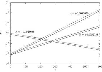
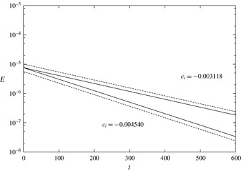
, respectively. Figure 4 compares the predicted growth rates with the kinetic energy of the flow computed with the DNS code, starting from an initial condition obtained by superposing the laminar solution and a perturbation of small enough amplitude to preserve linearity. It can be appreciated that stability theory and nonlinear numerical simulations produce exponential growth rates in very good agreement. For the most unstable case, at large times, one notices some small nonlinearities in the DNS curve, an effect that is obviously absent in the linear case. A similar plot is reported in figure 5 where, for validation purposes, two non-zero values of the momentum-transfer coefficient
 ${\it\tau}$
are considered for the case with
 $h_{p}=0.2$
: again, the numerical simulations compute (negative) growth rates of the perturbation energy which agree perfectly with the predictions from the linear stability theory.
Temporal evolution of the kinetic energy
 $E$
of disturbances for a channel flow over porous walls at
 $\mathit{Re}=2800$
. The porous layers have permeability
 ${\it\sigma}=0.004$
, porosity
 ${\it\varepsilon}=0.6$
and momentum-transfer coefficient
 ${\it\tau}=0$
. Dashed lines represent the evolution of energy as computed from stability theory, whereas solid lines represent evolution of energy as computed by the DNS code with
 $N_{y}=150$
(
 $N_{y,p}=75$
for
 $h_{p}=0.2$
and
 $N_{y,p}=250$
for
 $h_{p}=2$
). The three line sets refer to different thicknesses of the porous layer: for
 $h_{p}=0.2$
energy decays, for
 $h_{p}=1$
energy grows exponentially, and
 $h_{p}=2$
shows the largest growth rate.

Temporal evolution of the kinetic energy
 $E$
of disturbances for a channel flow over porous walls at
 $\mathit{Re}=2800$
. Flow parameters are the same as in figure 4 (
 $h_{p}=0.2$
) but for non-zero values of the parameter
 ${\it\tau}$
. When
 ${\it\tau}=-1$
the growth rate is
 $c_{i}=0.003118$
, and when
 ${\it\tau}=+1$
 $c_{i}=-0.004540$
.

3. The turbulent flow over a porous layer
We consider as a reference for our discussion a turbulent channel flow over impermeable walls, at
 $Re=2800$
, which corresponds to
 $Re_{{\it\tau}}\approx 180$
, the friction Reynolds number chosen by Kim et al. (Reference Kim, Moin and Moser1987) in their seminal DNS study. Bar discretization issues, the value of
 $Re$
is all that is needed to define the reference simulation of a channel flow bounded by two impermeable walls, whereas porous cases require additional quantities to describe the porous material: the thickness of the porous slab, its permeability and porosity, and the momentum-transfer coefficient that appears in the interface conditions.
All the simulations are performed at constant flow rate, so that the flow Reynolds number, defined by (2.1), is fixed at
 $Re=2800$
, where the bulk velocity is computed according to (2.2). One simulation is carried out at the higher value of
 $Re=6265$
, and is meant to explore how the main interfacial quantities change with Reynolds number. Owing to its increased computational cost, this case has been simulated on a domain of smaller spatial extension. For consistency, two low-
 $Re$
simulations at different permeabilities have also been recomputed by employing the smaller computational domain. As the focus of this work is the small-permeability regime, we first consider a baseline porosity case with a relatively small value of permeability and study its main turbulent quantities; the parameters of the porous material are then changed, one at a time, to gain a better insight into their relative importance in affecting the turbulent flow.
In the baseline case, the flow develops over two identical porous walls, whose height is
 $h_{p}=0.2$
; the dimensionless permeability of the porous material is
 ${\it\sigma}=0.004$
, its porosity is
 ${\it\varepsilon}=0.6$
, and the coefficient of the momentum-transfer conditions is
 ${\it\tau}=0$
. This set of parameters is rather classic, having being used in previous studies (Tilton & Cortelezzi Reference Tilton and Cortelezzi2006, Reference Tilton and Cortelezzi2008), the only peculiarity being the small value of
 ${\it\sigma}$
that reflects the present goal of investigating low-permeability materials. The value
 ${\it\sigma}=0.004$
has been determined in a precursory study (Quadrio et al.
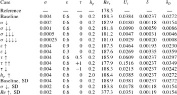
Reference Quadrio, Rosti, Scarselli and Cortelezzi2013) as an upper value of permeability where the linearity assumption in the porous layer is justified. The full set of simulations is reported in table 1, where the three cases computed in the smaller computational domain are denoted with SD. Table 1 also contains some mean quantities such as the resulting friction-based Reynolds number, the velocity at the interface, and a quantification of the wall-normal length scale related to the thickness of the boundary layer at the porous/fluid interface. In particular the quantity
 ${\it\delta}$
measures how fast the mean velocity profile changes from the interfacial velocity
 $U_{i}$
to the inner constant Darcy value
 $U_{D}$
, and is defined as the distance from the interface where the difference between the local velocity and
 $U_{D}$
reduces to
 $(1-1/\text{e})(U_{i}-U_{D})$
. On the other hand, the other length scale
 ${\it\delta}_{D}$
measures the position where the local mean velocity decreases to twice the value of
 $U_{D}$
.
Summary of the DNS performed at different porosity parameters, all at
 $Re=2800$
except the last one at
 $Re=6265$
. The baseline porosity case has
 ${\it\sigma}=0.004$
,
 ${\it\varepsilon}=0.6$
 ${\it\tau}=0$
and
 $h_{p}=0.2$
. SD indicates cases computed with a smaller computational domain (see text).

For all cases at
 $Re=2800$
, the equations of motion are discretized by using
 $256\times 256$
Fourier modes on a computational domain of
 $4{\rm\pi}\times 2{\rm\pi}$
in the streamwise and spanwise directions. In the wall-normal direction,
 $150$
grid points are used in the fluid region, and 75 points discretize the wall-normal derivatives in each porous slab (but
 $N_{y,p}=250$
in the case with
 $h_{p}=2$
). The spatial resolution of the numerical simulation is
 ${\rm\Delta}x^{+}\approx 8.8$
and
 ${\rm\Delta}z^{+}\approx 4.4$
, with a wall-normal resolution
 ${\rm\Delta}y^{+}$
that ranges from
 $0.16$
near the interface to
 $4.1$
in the centreline region of the channel. The size of the computational domain and the spatial resolution are comparable to those employed by Kim et al. (Reference Kim, Moin and Moser1987). The case at
 $Re=6265$
clearly has different discretization parameters: with a computational domain of
 $2{\rm\pi}\times {\rm\pi}$
in the wall-parallel directions, the same level of spatial resolution (in viscous units) is achieved with
 $N_{x}=256$
,
 $N_{z}=256$
, and
 $N_{y,p}=75$
, whereas
 $N_{y}$
is increased to
 $N_{y}=180$
.
Viscous units, which have been just used above to express spatial resolution, will often be employed in the following; they are indicated by the superscript
 $^{+}$
, and are built using the friction velocity
 $u_{{\it\tau}}$
as the velocity scale and the viscous length
 ${\it\delta}_{{\it\nu}}={\it\nu}/u_{{\it\tau}}$
as the length scale. For a turbulent channel flow with solid walls, the dimensionless friction velocity is defined as
 $$\begin{eqnarray}u_{{\it\tau}}=\sqrt{\frac{1}{\mathit{Re}}\left.\frac{\text{d}\,\overline{u}}{\text{d}y}\right|_{y=0}},\end{eqnarray}$$
where
 $\overline{u}$
is the mean velocity, obtained by time averaging
 $\tilde{u} (y,t)$
, and the subscript indicates that the derivative is taken at
 $y=0$
, the location of the solid wall. When the channel has porous walls, the above definition (3.1) must be modified to account for the turbulent shear stresses that are in general non-zero at the porous–fluid interface. We follow Breugem & Boersma (Reference Breugem and Boersma2005), and define
 $$\begin{eqnarray}u_{{\it\tau}}=\sqrt{\frac{1}{\mathit{Re}}\left.\frac{\text{d}\,\overline{u}}{\text{d}y}\right|_{y=0}-\left.\overline{u^{\prime }v^{\prime }}\right|_{y=0}},\end{eqnarray}$$
where
 $\overline{u^{\prime }v^{\prime }}$
is the off-diagonal component of the Reynolds stresses tensor, and the quantities are evaluated at the porous/fluid interface located at
 $y=0$
. At small-permeability values such as those considered in the present study, as seen in table 1, the value of the friction Reynolds number changes little from
 $\mathit{Re}_{{\it\tau}}\approx 180$
that characterizes the reference flow over impermeable walls.
All the simulations are started from an initial condition that requires some time for the flow to reach a state of statistical equilibrium. After such a state is reached, the calculations are continued for a time interval of 800 time units, during which 160 full flow fields are stored for further statistical analysis.
3.1. The baseline case
We start the comparison between the turbulent channel flows with porous or impermeable walls by analysing their mean properties. Small but finite effects of porosity can be appreciated already at a global energetic level: for example the value of
 $Re_{{\it\tau}}$
increases by approximately 5 % from
 $Re_{{\it\tau}}=178$
to
 $Re_{{\it\tau}}=188$
, with the skin-friction coefficient
 $C_{f}\equiv 2{\it\tau}_{w}/{\it\rho}U_{b}^{2}$
going up from
 $8.14\times 10^{-3}$
to
 $9.00\times 10^{-3}$
. As the simulations are carried out under the CFR condition, this implies that the power input to the system, given by the product of flow rate and mean pressure gradient, is correspondingly increased.
It is known that the skin-friction coefficient in a steady, fully developed, incompressible, plane channel flow under the CFR condition can be divided into a laminar and a turbulent contribution (Fukagata, Iwamoto & Kasagi Reference Fukagata, Iwamoto and Kasagi2002), via the so-called FIK identity. When the fluid flows over porous walls, additional terms arise which indicate how the porous material affects the turbulent friction. To identify these additional terms, we start from the streamwise component of the incompressible momentum equation, which after being averaged in time and along the homogeneous directions becomes
 $$\begin{eqnarray}\frac{\partial \overline{p}}{\partial x}=\frac{\partial }{\partial y}\left(\frac{1}{Re}\frac{\partial \overline{u}}{\partial y}-\overline{u^{\prime }v^{\prime }}\right).\end{eqnarray}$$
Based on the definition (3.2) of the friction velocity, the friction coefficient is defined as
 $$\begin{eqnarray}C_{f}=2\left(\frac{1}{Re}\left.\frac{\partial \overline{u}}{\partial y}\right|_{y=0}-\left.\overline{u^{\prime }v^{\prime }}\right|_{y=0}\right).\end{eqnarray}$$
Integrating (3.3) from
 $y=0$
to
 $y=1$
and noting that both
 $\partial \overline{u}/\partial y$
and
 $\overline{u^{\prime }v^{\prime }}$
are zero at the centreline for symmetry reasons, a relation between the pressure gradient and the skin-friction coefficient (3.4) is obtained, i.e.
 $$\begin{eqnarray}-\frac{\partial \overline{p}}{\partial x}=\frac{C_{f}}{2}.\end{eqnarray}$$
Substituting (3.5) into (3.3) we obtain
 $$\begin{eqnarray}\frac{C_{f}}{2}=\frac{\partial }{\partial y}\left(\overline{u^{\prime }v^{\prime }}-\frac{1}{Re}\frac{\partial \overline{u}}{\partial y}\right).\end{eqnarray}$$
Integrating the above equation (3.6) twice from
 $0$
to
 $y$
leads to
 $$\begin{eqnarray}\frac{C_{f}}{2}\left(y-\frac{y^{2}}{2}\right)=\int _{0}^{y}-\overline{u^{\prime }v^{\prime }}\,\text{d}y+\frac{1}{Re}\left(\overline{u}-U_{i}\right),\end{eqnarray}$$
where
 $U_{i}$
indicates the mean velocity at the interface. A further integration in
 $y$
from
 $0$
to
 $1$
gives
 $$\begin{eqnarray}\frac{C_{f}}{6}=\int _{0}^{1}\int _{0}^{y}-\overline{u^{\prime }v^{\prime }}\,\text{d}y\,\text{d}y+\frac{1}{Re}\left(\int _{0}^{1}\overline{u}\,\text{d}y-U_{i}\right).\end{eqnarray}$$
and a subsequent integration by parts gives
 $$\begin{eqnarray}\displaystyle \int _{0}^{1}\int _{0}^{y}-\overline{u^{\prime }v^{\prime }}\,\text{d}y\,\text{d}y & = & \displaystyle \left[y\int _{0}^{1}-\overline{u^{\prime }v^{\prime }}\,\text{d}y\right]_{0}^{1}-\int _{0}^{1}y(-\overline{u^{\prime }v^{\prime }})\,\text{d}y\nonumber\\ \displaystyle & = & \displaystyle \int _{0}^{1}-\overline{u^{\prime }v^{\prime }}\,\text{d}y-\int _{0}^{1}y(-\overline{u^{\prime }v^{\prime }})\,\text{d}y,\end{eqnarray}$$
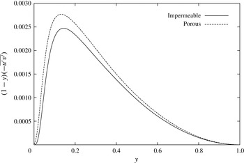
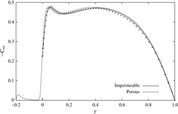
Wall-normal profile of the integrand of the second term in the FIK identity (3.10) for the impermeable and porous cases.

and leads to the following extended FIK identity for a turbulent channel flow with porous wall:
 $$\begin{eqnarray}C_{f}=\frac{6}{Re}\int _{0}^{1}\overline{u}\,\text{d}y+6\int _{0}^{1}(1-y)(-\overline{u^{\prime }v^{\prime }})\,\text{d}y-\frac{6}{Re}U_{i}.\end{eqnarray}$$
This relation states that the skin friction is the sum of three different contributions. The laminar contribution (first term) is identical to the case of an impermeable wall. The second term is formally identical to the impermeable one, but the non-zero boundary value of the shear stress at
 $y=0$
must be remembered. Lastly, the third term accounts for the mean slip velocity at the interface. This extended FIK identity, which reduces to the standard one for impermeable walls, is well verified by the present data, as the value of
 $C_{f}=0.0090$
computed via (3.10) is identical to that obtained by using its definition and the expression (3.2) for the friction velocity. The laminar, turbulent and interface velocity contributions are
 $0.0021$
,
 $0.0068$
and
 $8.2\times 10^{-5}$
. In comparison to the impermeable case, the laminar term is identical, obviously the interfacial velocity term is zero, and the Reynolds stress term is
 $0.0060$
. Figure 6 illustrates the weighted wall-normal profile of the Reynolds-shear stress, i.e. the integrand in the second term of (3.10), in comparative form between the impermeable and porous cases. The porous integrand is larger than the impermeable wall throughout the whole channel. The case at higher
 $Re$
has laminar, turbulent and interface velocity contributions equal to
 $0.00096$
,
 $0.00627$
and
 $0.00003$
, respectively.
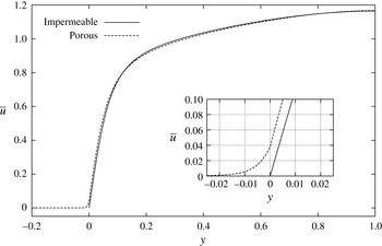
Comparison of the mean velocity profile
 $\overline{u}$
of turbulent channel flow at
 $\mathit{Re}=2800$
, over an impermeable wall (reference case, solid line) and a porous wall (baseline case, dashed line). The thickness of the porous layer is
 $h_{p}=0.2$
, the permeability is
 ${\it\sigma}=0.004$
, the porosity is
 ${\it\varepsilon}=0.6$
and the coefficient in the momentum-transfer conditions is
 ${\it\tau}=0$
. The inset shows the zoomed-in interfacial region where the porous profile exhibits a non-zero slip velocity.

Figure 7 shows the wall-normal distribution of the streamwise component of the mean velocity, in comparative form for the channel flow over impermeable and porous walls. The two profiles are quite similar throughout the channel, and reach their maximum at the centreline with
 $\overline{u}(1)=1.165$
, with the difference being that the porous velocity is slightly higher in the region near the interface, and consequently lower (owing to the constraint of constant flow rate) in the outer region, with the crossover taking place at
 $y\approx 0.15$
. A zoomed view of the velocity profile near the interface between the fluid region and the porous layer is shown in the inset of figure 7, where a slip velocity of approximately
 $U_{i}=0.038$
is observed at the interface. The mean velocity within the porous material is strictly zero only at the impermeable wall located at
 $y=-0.2$
, and assumes an essentially constant value in the bulk of the porous layer. This value equals the Darcy velocity
 $U_{D}^{\ast }=-K^{\ast }/{\it\mu}^{\ast }\,\text{d}\overline{p^{\ast }}/\text{d}x^{\ast }$
, which in the present case in dimensionless form is
 $U_{D}=1.97\times 10^{-4}$
. As the interface at
 $y=0$
is approached, the fluid velocity within the porous material increases further from the Darcy value to the interfacial velocity
 $U_{i}$
, and this process takes place in a thin layer, whose thickness
 ${\it\delta}$
turns out to be
 $0.00237$
when computed as the distance from the interface to the location where the local velocity becomes
 $1-1/\text{e}\approx 63\,\%$
of
 $U_{i}-U_{D}$
. The velocity profile on the two sides of the interface has different slopes, and this, together with a non-zero interfacial shear stress for the porous case, explains the different values of the friction Reynolds number.
Comparison of the mean velocity minus the interface velocity,
 $(\overline{u}-U_{i})^{+}$
, versus the distance from the interface,
 $y^{+}$
. The profiles for an impermeable wall (reference case, solid line) and a porous wall (baseline case, dashed line) are compared with the mean profile from Kim et al. (Reference Kim, Moin and Moser1987) (symbols). Dash-dotted lines indicate
 $\overline{u}^{+}-U_{i}^{+}=y^{+}$
and
 $\overline{u}^{+}-U_{i}^{+}=2.5\ln y^{+}+5.5$
.

Figure 8 compares the mean velocity profiles in the fluid region only. Following Hahn et al. (Reference Hahn, Je and Choi2002), the profiles are plotted as the difference
 $(\overline{u}-U_{i})^{+}$
versus the logarithm of the distance from the interface
 $y^{+}$
; both quantities are expressed in wall units. The mean velocity profile computed by Kim et al. (Reference Kim, Moin and Moser1987) is also added, and turns out to be undistinguishable from the present results for the impermeable wall. The velocity profile over the porous wall possesses the three regions that are present in the standard channel flow: the viscous sublayer for
 $y^{+}<5$
, the logarithmic region for
 $y^{+}>30$
, and the buffer layer in between. In the logarithmic region,
 $$\begin{eqnarray}\left(\overline{u}-U_{i}\right)^{+}=\frac{1}{{\it\kappa}}\ln y^{+}+B^{+},\end{eqnarray}$$
where
 ${\it\kappa}$
and
 $B^{+}$
are two constants whose values (at this value of
 $\mathit{Re}$
) are
 ${\it\kappa}=0.4$
and
 $B^{+}=5.5$
. When plotted in the law-of-the-wall form, the only significant difference exhibited by the porous profile is in the logarithmic region, where the curve is significantly lower than the case with solid walls (a fit with
 ${\it\kappa}=0.4$
yields
 $B^{+}=4$
). These results are in line with those by Hahn et al. (Reference Hahn, Je and Choi2002) and by Breugem et al. (Reference Breugem, Boersma and Uittenbogaard2006). The former mimicked the effects of the porous layer through a suitable set of boundary conditions applied at the interface, and found a logarithmic law with unchanged slope and decreased constant, indicating a reduced thickness of the viscous sublayer. The latter presented a detailed discussion of the mean velocity profile but, as mentioned in the Introduction, their method for characterizing the porous material is such that a direct, quantitative comparison between their cases and the present results is not possible. However, they also conclude that at low permeabilities the slope of the velocity profile is unaffected.
R.m.s. values of velocity fluctuations, expressed in wall units, as a function of the distance
 $y^{+}$
from the interface, for a turbulent channel flow at
 $\mathit{Re}=2800$
. Solid and dashed lines indicate the flow over porous and impermeable walls, respectively. Symbols are for the impermeable case from Kim et al. (Reference Kim, Moin and Moser1987).

We continue our comparison between the turbulent channel flows with porous or impermeable walls by analysing the wall-normal distribution of r.m.s. values of velocity fluctuations. Figure 9 shows their profiles (including data from Kim et al. (Reference Kim, Moin and Moser1987), which overlap with the present results for the impermeable wall); they are affected by the porous walls, and the effect is not limited to the interfacial region, but extends up to 80–100 wall units. All the components for the porous case present non-null r.m.s. values at
 $y=0$
, where the no-slip condition is not enforced, but they decrease quickly inside the porous layer. In relative terms, the wall-normal and spanwise components are probably the most affected, with the position of their peaks moving towards the interface, a shift attributed by Perot & Moin (Reference Perot and Moin1995) to the decreased blocking and viscous effects exerted by the porous wall.
Figure 10 depicts how the r.m.s. intensity of velocity fluctuations change within the porous material from the small but non-zero interfacial value down to zero at the solid wall. At the interface the
 $v$
component is the smallest and the
 $u$
component is the largest; inside the porous slab, the wall-parallel components drop to a nearly constant value, and become nearly indistinguishable from each other, decreasing very slowly and eventually dropping to zero across a very thin small wall layer. The
 $v$
component, on the other hand, presents a markedly lower decay rate and is the largest one for
 $-0.08<y<0.02$
. The asymptotic behaviour as the solid wall is approached is linear for the wall-parallel components, and quadratic for the wall-normal one, as required by the no-slip boundary condition and continuity equations. This very presence of velocity fluctuations demonstrates that, strictly speaking, the VANS-filtered flow inside the porous slab is not fully laminar, although the magnitude of the fluctuations is small. The structure of this non-laminar flow, however, is different from turbulence inside the channel, as will be seen in the following.
R.m.s. values of velocity fluctuations, expressed in wall units, within the porous slab.

Correlation coefficient
 $C_{uv}$
between the streamwise and wall-normal velocity fluctuations for a turbulent flow at
 $\mathit{Re}=2800$
. Solid and dashed lines indicate the flow over impermeable and porous walls, respectively. Symbols are for the impermeable case from Kim et al. (Reference Kim, Moin and Moser1987).

Figure 11 effectively illustrates how the structure of the (small) turbulent fluctuations changes across the porous layer, by plotting the wall-normal profile of the correlation coefficient
 $-C_{uv}$
between the fluctuations of the streamwise and wall-normal velocity components, i.e. the off-diagonal component of the Reynolds stress tensor made dimensionless by the local
 $u_{rms}v_{rms}$
. The value of
 $-C_{uv}$
is zero in the isotropic case and is also zero at the centreline; it retains a rather large value, between 0.4 and 0.5, in most of the channel gap, as in the impermeable case; then presents a small local peak near the wall and then decreases to approximately 0.2 as the wall is approached in the impermeable case. Near the interface with the porous medium, on the channel side
 $-C_{uv}$
is almost unaffected by porosity, with only the local peak being slightly moved towards the interface; from the interface down
 $-C_{uv}$
decreases rather quickly to zero. For most of the porous layer it remains nearly zero, but when the solid wall is approached
 $-C_{uv}$
progressively increases again, shows a local peak at
 $y\approx -0.18$
, i.e. at a distance of
 $0.02$
from the solid wall, and then eventually drops to zero. Hence, regardless of the presence of the porous material and of the limited intensity of velocity fluctuations, the peak is due to the presence of the solid wall.
R.m.s. values of vorticity fluctuations, expressed in wall units, as a function of the distance
 $y^{+}$
from the interface, for a turbulent channel flow at
 $\mathit{Re}=2800$
. Solid and dashed lines indicate the flow over impermeable and porous walls, respectively. Symbols are for the impermeable case from Kim et al. (Reference Kim, Moin and Moser1987).

Figure 12 shows the profiles of the r.m.s. intensities of vorticity fluctuations. Again, available data from Kim et al. (Reference Kim, Moin and Moser1987) are plotted for comparison, and overlap very well with the present results for the impermeable wall. Similarly to the velocity fluctuations, a non-trivial effect of the porous wall upon the vorticity fluctuations can be observed: the spanwise component is the largest as in the impermeable case and is increased near the interface, but its intensity becomes lower for
 $4<y^{+}<50$
. The streamwise component is slightly decreased for
 $y^{+}<3$
and increased outwards, while the wall-normal component behaves similarly to the spanwise one, being increased for
 $y^{+}<10$
and slightly decreased for
 $10<y^{+}<50$
. In particular the local peak of
 ${\it\omega}_{x}$
fluctuations at
 $y^{+}\approx 20$
, often associated (Kim et al.
Reference Kim, Moin and Moser1987) with the average wall-normal position of quasi-streamwise vortical structures, seems to be only slightly affected by the porous material, at least at this level of permeability. In agreement with Breugem et al. (Reference Breugem, Boersma and Uittenbogaard2006), it can be inferred that the near-wall structure of the turbulent flow is affected too, as this peak is connected with the presence of high- and low-velocity streaks.
Low- and high-velocity near-wall streaks in the turbulent flow over an impermeable wall (a) and over a porous wall (b). The streaks are visualized via blue/red isosurfaces for
 $u^{\prime +}=\pm 4$
for the lower half of the channel. The more fragmented nature of the streaky structures over the porous material is evident.

Changes, albeit small, in the near-wall structure of the flow are indeed visually confirmed by figure 13, which shows the elongated low- and high-velocity near-wall streaks, plotted as isosurfaces where the local velocity assumes the values
 $u^{\prime +}=\pm 4$
. The small value of permeability notwithstanding, near the porous wall the structures appear as less elongated and more fragmented, especially those parts of the low-speed streaks that are located near the interface. This information will be statistically assessed later.
Contour levels of the
 $u$
(colour map) and
 $v$
(isolines) fluctuating fields at the interface
 $y=0$
for the baseline porous case. Enlarged view of a limited portion of the wall, with flow from left to right. Colour bands for
 $u$
are (
 $-0.01,0.02,0.15$
) from blue/dark to red/light. Contour increments for
 $v$
are (
 $-0.025,0.01,0.045$
), with dashed lines for negative contours.

A further look at the interface plane, shown in figure 14, amplifies these differences, and demonstrates that the flow is rich in small-scale features, consistent with a picture where the larger coherent structures are being broken into smaller pieces by the porous material. Here the streamwise and wall-normal fluctuating velocity fields are visualized; at the interface both show relatively small fluctuations. The structure of the large-scale low- and high-speed streaks can still be discerned, but the streaks (especially the low-speed ones) are fragmented into smaller structures; at the interface positive fluctuations of
 $v$
(i.e. related to pockets of fluid being ejected outwards towards the bulk flow) are stronger than negative ones.
Wall-normal profile of the dissipation
 ${\it\epsilon}$
of the fluctuating field, for a turbulent channel flow at
 $\mathit{Re}=2800$
. Solid and dashed line indicate the flow over impermeable and porous walls, respectively. In (a) the quantities are scaled in outer units, while (b) employs inner units.

This increased fragmentation is likely to increase viscous dissipation. Figure 15 plots the wall-normal profile of the dissipation
 ${\it\epsilon}={\it\mu}\overline{\partial _{j}u_{i}^{\prime }\partial _{j}u_{i}^{\prime }}$
of the fluctuating velocity field. While the general aspect of the curve in the porous case (figure 15
a) resembles that of the impermeable case, a larger dissipation is evident over a significant range of distances from the interface, say
 $y<0.4$
, and in particular the value at the interface is much larger. Dissipation then drops to zero very quickly in the porous layer, as velocity fluctuations are damped by the porous material, and remains negligible down to the solid wall. Most of the large differences, however, are simply a consequence of the two flows possessing slightly different values of friction Reynolds number
 $Re_{{\it\tau}}$
. Figure 15(b) emphasizes the much better match between the two curves in the bulk region when inner scaling is adopted to account for the change in
 $Re_{{\it\tau}}$
. At the interface with the porous medium, dissipation is still observed to assume larger values (although the increase is much smaller), but this increase is counterbalanced by a slight decrease in the outer part, say for
 $3<y^{+}<50$
. When expressed in wall units and integrated along the wall-normal direction, the turbulent dissipation is only slightly reduced in the porous case.
Quadrio (Reference Quadrio2011) and Ricco et al. (Reference Ricco, Ottonelli, Hasegawa and Quadrio2012) introduced the concept of the energy box to illustrate the energy flux through the channel flow system, linking energy input per unit time to total energy dissipation, i.e. the sum of turbulent dissipation and the dissipation ascribed to the mean velocity profile. In the present case, where no active flow control device is present, energy enters the system through the pumping action (product of flow rate and pressure gradient), and in statistical equilibrium this energy input must balance the sum of turbulent dissipation and direct dissipation from the mean profile. It is known (Laadhari Reference Laadhari2007) that at low values of
 $Re$
the latter mechanism is a significant one, and indeed in our case the mean profile accounts for slightly more than one half of the total dissipation. The power input in the baseline porous case, however, when expressed in wall units is less than that of the reference case, as the flow rate is kept constant in outer units and the friction velocity is larger over the porous wall, hence the flow rate in inner units decreases. This implies that turbulent dissipation, while slightly decreased in wall units and in absolute terms, does in the porous case account for a larger share of the entire dissipation.
The Lumley triangle, for a turbulent channel flow at
 $\mathit{Re}=2800$
.
 $-\text{II}$
and III are the second and third invariant of the Reynolds stress anisotropy tensor, and the bounding line shows the region of admissible turbulence states, amid the extremal states of one-component turbulence (1C), two-component turbulence (2C), axisymmetric turbulence (axi), two-component axisymmetric turbulence (2C axi) and isotropic turbulence (iso). Solid and dashed line indicate the flow over impermeable and porous walls, respectively. The triangles correspond to
 $y=0$
and the square to
 $y=-h_{p}$
. The circle marks the nearly isotropic state, which is visited by the flow for
 $y=1$
and, for the porous case, also in the bulk of the porous layer.

One-dimensional autocorrelation function for the velocity fluctuations for a turbulent channel flow at
 $\mathit{Re}=2800$
. (a,c)
 $y^{+}\approx 5$
, (b,d)
 $y^{+}\approx 150$
; (a,b) streamwise separation, (c,d) spanwise separation.

A similar picture emerges from the analysis of the anisotropy invariant map (AIM), also called Lumley triangle, shown in figure 16. The AIM is a plot on the plane of the second and third invariant of the Reynolds stress anisotropy tensor; in this plane, a region is delimited by an approximately triangular boundary whose sides correspond to special limiting states of the turbulent flow. In the case of impermeable channel flow, represented by a solid line, one moves along the line as the wall-normal position changes, with the centreline corresponding to an almost isotropic state near the origin of the plane, and the very-near-wall region corresponding to the part of the curve near the upper boundary of the triangle. Here the boundary curve corresponds to a two-component turbulence, as it should be in close proximity of a solid wall. The curve for the porous case is nearly identical to the reference one for most of the wall-normal positions, with the exception of the region very near to the interface. Here the porous curve does not follow closely the upper boundary and bends downward, reflecting the structural changes induced by the porous material. The differences between the two curves, however, are limited to a rather thin layer, and disappear for say
 $y^{+}>5$
. Below the interface, the turbulent state further departs from the two-component boundary, and quickly reaches the origin of the plane, corresponding to the isotropic state. It then remains near the origin until the boundary layer over the solid wall is reached: at that point the flow state moves from the origin towards the left corner, which represents the two-dimensional isotropic state.
These differences, confined within a thin region above the interface, possess dynamical consequences that extend further into the fluid region. This was visually evident, for example, already in the instantaneous flow fields presented in figures 13 and 14, where low-speed and high-speed velocity streaks are shown to be more fragmented throughout their whole wall-normal extension. A similar message is conveyed by figure 17, which shows the two-point autocorrelation functions for the velocity fluctuations, as a function of either the streamwise or the spanwise separation. In the outer region of the channel the curves are almost identical, but at
 $y^{+}=5$
(a,c) the autocorrelations, although qualitatively similar between the two flows, distinctly show how the porous wall affects the spatial coherency of the structures, reflected by the elongation of the correlation functions. Note that at such a distance from the interface the structural differences just highlighted by the AIM have already vanished. The fact that spanwise correlations are marginally affected, but longitudinal correlations are consistently shorter in the near-wall region, confirms similar results already obtained by Breugem et al. (Reference Breugem, Boersma and Uittenbogaard2006) and extends them to the present, much lower value of permeability
 ${\it\sigma}=0.004$
, for which the wall is generally believed to be effectively impermeable.
Two-dimensional autocorrelation functions for the velocity components
 $u$
(a),
 $v$
(b) and
 $w$
(c), for a turbulent channel flow at
 $\mathit{Re}=2800$
, at the centre plane
 $y=-0.1$
of the porous layer. Contours from 0.95 by 0.1 decrements, negative levels are plotted with dashed lines.

The flow inside the porous layer, although characterized by small velocity fluctuations, possesses a well-defined structure. We exemplify it with figure 18, which features the wall-parallel two-dimensional autocorrelation function for the three velocity components in the middle of the porous layer, i.e. at
 $y=-0.1$
. Although corresponding to small energetic levels, these interesting patterns present relatively large spanwise scales and suggest the presence of a streamwise length scale (distance of the minimum from the origin) of approximately 90 viscous units (or
 $x/h\approx 0.5$
) for both the streamwise and wall-normal correlations. Even at the present small levels of permeability we thus find a statistical signature of the spanwise vortical structures or rolls that have been already identified over significantly more porous walls (Breugem et al.
Reference Breugem, Boersma and Uittenbogaard2006), rough surfaces (Jiménez et al.
Reference Jiménez, Uhlmann, Pinelli and Kawahara2001) and plant canopies (Finnigan Reference Finnigan2000), and are suggested (Garcia-Mayoral & Jiménez Reference Garcia-Mayoral and Jiménez2011) to be the main cause of performance loss of drag-reducing riblets when the riblets size is increased above their optimum. The footprints of such structures reach deep into the porous material.
One-dimensional autocorrelation function for the velocity components
 $u$
(a),
 $v$
(b) and
 $w$
(c), for a turbulent channel flow at
 $\mathit{Re}=2800$
, at zero spanwise and wall-normal separations. The autocorrelations at different
 $y$
are plotted together, and the dashed-dotted line indicates the position of the interface. Contours from 0.95 by 0.1 decrements, negative levels are plotted with dashed lines.

Figure 19 illustrates how the structure of the correlation functions change along the wall-normal direction. First, it should be noted explicitly that the figure stacks one-dimensional longitudinal correlations in the
 $y$
direction. In the channel region the correlations, and in particular that for the streamwise component, present relatively large length scales, related to the elongated streaky structures that characterize the near-wall region, although from figure 14 one deduces that for the porous case the typical length scales are slightly reduced. Then the correlations change rapidly but continuously across the interface, and the length scale becomes much shorter for the
 $u$
component inside the porous material, which cannot support the streak structures, while remaining comparable to the channel length scales for the other two components. We also recover in the present small-permeability case the result, described by Breugem et al. (Reference Breugem, Boersma and Uittenbogaard2006), that the correlations present an alternating sequence of progressively weaker negative and positive local peaks. These peaks, although barely noticeable at these levels of permeability, indicate a streamwise periodic organization of the flow structures that Breugem et al. (Reference Breugem, Boersma and Uittenbogaard2006) related to large-scale pressure fluctuations within the porous material.
Profile of the mean velocity minus the interface velocity,
 $(\overline{u}-U_{i})^{+}$
, plotted versus the distance
 $y^{+}$
from the interface. The baseline case with permeability
 ${\it\sigma}=0.004$
(thick dashed line) is compared with decreasing values of
 ${\it\sigma}$
and to the impermeable wall (continuous line). Dash-dotted lines indicate
 $\overline{u}^{+}-U_{i}^{+}=y^{+}$
and
 $\overline{u}^{+}-U_{i}^{+}=2.5\ln y^{+}+5.5$
.

3.2. Effect of porosity parameters
Permeability
 ${\it\sigma}$
is arguably the most important parameter of a porous material. Besides the reference value
 ${\it\sigma}=0.004$
, four smaller values are considered, as per table 1. It can be seen that in all cases the skin friction (hence the value of
 $Re_{{\it\tau}}$
) increases with respect to the reference flow, but the increase tends to zero as
 ${\it\sigma}$
becomes smaller. Similarly to figure 8, figure 20 shows the mean velocity profile in law-of-the-wall form, where distance
 $y$
from the interface and mean velocity
 $(\overline{u}-U_{i})$
after removal of the interface velocity contribution are plotted in wall units. The velocity profile with this choice of non-dimensionalization is unchanged in the near-wall portion. In the log layer the slope of the profile is unaltered, while the intercept increases with decreasing values of
 ${\it\sigma}$
and approaches, as expected,
 $B^{+}=5.5$
for vanishing
 ${\it\sigma}$
. Hence, as the wall friction converges towards the impermeable case, the profiles monotonically approach the standard wall law that is valid for a turbulent channel flow over solid walls. Values of permeability of the order of
 $10^{-4}$
can thus be considered the practical limit below which a porous wall behaves like a solid wall in terms of mean quantities. It is interesting to note that the effects of permeability, at these small values, on the mean velocity profile of the turbulent channel flow at
 $Re=2800$
are quantitatively similar to effects of permeability on the velocity profile of a laminar pressure-driven channel flow at
 $Re=3000$
(Tilton & Cortelezzi Reference Tilton and Cortelezzi2008), where
 ${\it\sigma}=0.0002$
can be considered the practical limit below which a porous wall behaves like a solid wall in terms of linear stability.
R.m.s. values of velocity fluctuations, expressed in wall units, as a function of the distance
 $y^{+}$
from the interface, and correlation coefficient
 $C_{uv}$
between the streamwise and wall-normal velocity fluctuations. The baseline case with permeability
 ${\it\sigma}=0.004$
(thick dashed line) is compared to cases with decreasing values of
 ${\it\sigma}$
and to the impermeable wall. The curves for the lowest permeability values of
 ${\it\sigma}=0.0005$
and
 ${\it\sigma}=0.00025$
are not shown as they overlap the curves for the impermeable case.

A consistent picture is obtained by plotting the turbulence fluctuations, see figure 21. The profiles for the r.m.s. values of the velocity components as well as the correlation coefficient
 $-C_{uv}$
confirm that the statistics of the flow do converge towards those of the impermeable wall for decreasing values of
 ${\it\sigma}$
. For these second-order moments, the limiting value of permeability below which differences can no longer be noticed is
 ${\it\sigma}=0.001$
, i.e. larger than the limit value for the mean velocity profile.
R.m.s. values of velocity fluctuations at the interface, for different values of permeability
 ${\it\sigma}$
.

Figure 22 shows, for each component of the velocity vector, how the r.m.s. value of the fluctuations at the interface increases as a function of
 ${\it\sigma}$
. A more than linear increase is observed, with the longitudinal component being the largest and the wall-normal component the smallest for a given
 ${\it\sigma}$
. In comparing with figures 11 and 12 by Breugem et al. (Reference Breugem, Boersma and Uittenbogaard2006), similar trends can be observed, but here the fluctuations are two orders of magnitude smaller, owing to the much smaller permeability of the material.
One-dimensional autocorrelation function for the three velocity components, for a turbulent channel flow at
 $\mathit{Re}=2800$
, at
 $y^{+}\approx 5$
. The baseline case with permeability
 ${\it\sigma}=0.004$
(thick dashed line) is compared to cases with decreasing values of
 ${\it\sigma}$
and to the impermeable wall. The curves for the lowest permeability values of
 ${\it\sigma}=0.0005$
and
 ${\it\sigma}=0.00025$
are not shown as they overlap the curves for the impermeable case.

The two-point velocity correlations are pictured in figure 23. In particular, even the longitudinal autocorrelation function for the streamwise velocity fluctuations, which is the most affected by the porous material, as shown in figure 17, becomes indistinguishable from the reference case of a channel flow over an impermeable wall for
 ${\it\sigma}<0.001$
, thus confirming that this can be taken as the practical limit below which porosity effects are negligible, as far as second moments are concerned.
Profile of the mean velocity minus the interface velocity,
 $(\overline{u}-U_{i})^{+}$
, plotted versus the distance from the interface
 $y^{+}$
. The baseline case with porosity
 ${\it\varepsilon}=0.6$
(dashed line) is compared to larger, 0.9 (thick dotted line), and smaller, 0.3 (thin dotted line), values of
 ${\it\varepsilon}$
and to the impermeable wall (solid line). Dash-dotted lines indicate
 $\overline{u}^{+}-U_{i}^{+}=y^{+}$
and
 $\overline{u}^{+}-U_{i}^{+}=2.5\ln y^{+}+5.5$
.

Aside from permeability, porosity,
 ${\it\varepsilon}$
, is the other parameter that characterizes a porous material. At odds with permeability, the amount of porosity does not affect turbulence statistics in a significant way. A quick look at the mean velocity profiles in figure 24 shows that further increasing
 ${\it\varepsilon}$
above the baseline value of
 ${\it\varepsilon}=0.6$
has little or no effect on the mean profile, whereas halving the porosity value shifts the logarithmic part of the velocity profile towards the one for the impermeable wall, but the shift is minimal. A similar picture emerges after examining other quantities (not shown), such as the wall-normal profiles of velocity fluctuations, correlations and spectra. Overall, this suggests that the limiting behaviours of
 ${\it\varepsilon}$
and
 ${\it\sigma}$
are quite different. The effects of porosity, at these small values of permeability, on the mean velocity profile of the turbulent channel flow at
 $Re=2800$
are again quantitatively similar to the effects of porosity on the velocity profile of a laminar pressure-driven channel flow at
 $Re=3000$
(Tilton & Cortelezzi Reference Tilton and Cortelezzi2008).
The effects of the momentum-transfer coefficient
 ${\it\tau}$
on the turbulence statistics are now considered. To understand the importance of the role played by the parameter
 ${\it\tau}$
, one should envision the changes in the values of
 ${\it\sigma}$
and
 ${\it\epsilon}$
as one moves from deep down in the porous material, up to the fluid/porous interface and into the fluid. Deep inside the porous materials the values of
 ${\it\sigma}$
and
 ${\it\epsilon}$
are the bulk values representative of the porous material chosen. Approaching the interface the values of
 ${\it\sigma}$
and
 ${\it\epsilon}$
change rapidly from their bulk values to
 ${\it\sigma}=\infty$
and
 ${\it\epsilon}=1$
in the fluid just above the interface. The change takes place in the porous material in a thin transition layer adjacent to the interface, and the functional variation of
 ${\it\sigma}$
and
 ${\it\epsilon}$
depends mainly on the porosity of the material and on how the interface has been machined (see figure 1).
Profile of the mean velocity minus the interface velocity,
 $(\overline{u}-U_{i})^{+}$
, plotted versus the distance
 $y^{+}$
from the interface. The baseline case with momentum-transfer coefficient
 ${\it\tau}=0$
(dashed line) is compared to the impermeable wall (solid line) and to the cases with
 ${\it\tau}=-1$
,
 ${\it\tau}=0.5$
and
 ${\it\tau}=+1$
.

In this study, however, we focus on porous materials of small permeabilities and small mean particle sizes. In particular, for sufficiently low permeabilities, the fluid velocity at the porous/fluid interface is small; the convective effects, and consequently the drag force experienced by the fluid, become negligible, because the dense channel-like structures of the porous matrix impede motion between layers of fluid. In this case, the transition region (of the order of a few pore diameters thick) and roughness (of the order of one pore diameter high) can be assumed to have zero thickness, and porosity and permeability to have a constant value up to an interface that has a clearly defined position (Ochoa-Tapia & Whitaker Reference Ochoa-Tapia and Whitaker1995a
, Reference Ochoa-Tapia and Whitaker1998; Valdés-Parada et al.
Reference Valdés-Parada, Goyeau and Ochoa-Tapia2007; Valdés-Parada et al.
Reference Valdés-Parada, Aguilar-Madera, Ochoa-Tapia and Goyeay2013). Therefore, following Ochoa-Tapia & Whitaker (Reference Ochoa-Tapia and Whitaker1995a
), we model the effects of the variation of
 ${\it\sigma}$
and
 ${\it\epsilon}$
in the transition layer using the momentum-transfer coefficient
 ${\it\tau}$
(see the interface conditions (2.22) and (2.23)). The parameter
 ${\it\tau}$
, as suggested by Minale (Reference Minale2014a
,Reference Minale
b
), models the transfer of stress at the porous/fluid interface. This dimensionless parameter is of the order of one and can be both positive or negative, depending on the type of porous material considered and the type of machining of the interface (Ochoa-Tapia & Whitaker Reference Ochoa-Tapia and Whitaker1998). In the case when
 ${\it\tau}=0$
, the stress carried by the free flowing fluid is fully transferred to the fluid saturating the porous matrix, a negative
 ${\it\tau}$
quantifies the amount of stress transferred from the free fluid to the porous matrix, while a positive
 ${\it\tau}$
quantifies the amount of stress transferred from the porous matrix to the free fluid. Note that, in our model, the momentum-transfer coefficient is decoupled from both porosity and permeability and, therefore, its effects can be assessed independently. In order to model a wide range of porous materials and surface machining, we follow Tilton & Cortelezzi (Reference Tilton and Cortelezzi2008) and discuss the effects of the momentum-transfer coefficient as it varies between
 $-1$
and
 $+1$
. In particular, we consider four values of
 ${\it\tau}=-1,0,0.5$
and 1, because Tilton & Cortelezzi (Reference Tilton and Cortelezzi2008) showed that positive values of
 ${\it\tau}$
have a strong nonlinear effect on the linear stability of a pressure-driven flow in a channel with porous wall.
Figure 25 presents the mean velocity profiles for the four considered values of the momentum-transfer coefficient. The nonlinear effects of
 ${\it\tau}$
on the mean velocity profile are quite evident: while the mean velocity profiles for the cases
 ${\it\tau}=-1$
, 0, and 0.5 are grouped together, the case
 ${\it\tau}=1$
induces a significant increase of the mean profile at the interface, and a consequent decrease in the central region of the channel owing to the constant flow rate constraint. The effects of
 ${\it\tau}$
, at these small values of permeability, on the mean velocity profile of the turbulent channel flow at
 $Re=2800$
are again quantitatively similar to the effects of
 ${\it\tau}$
on the velocity profile of a laminar pressure-driven channel flow at
 $Re=3000$
(Tilton & Cortelezzi Reference Tilton and Cortelezzi2008). Also the wall-normal derivatives of the mean velocity profile at the interface are significantly and nonlinearly affected by the value of
 ${\it\tau}$
, with the friction velocity
 $u_{{\it\tau}}$
being larger when
 ${\it\tau}=-1$
and smaller when
 ${\it\tau}=0.5$
, and much smaller when
 ${\it\tau}=1$
compared to the baseline case (
 ${\it\tau}=0$
). As reported in table 1,
 ${\it\tau}=1$
yields a wall friction which is down to the value of the impermeable wall. This unexpected result is supported by further information presented below. Note, however, that for
 ${\it\tau}=1$
the interfacial velocity is approximately four times larger than the baseline case, and this could hinder the linearity assumption in the porous layer; therefore, quantitative considerations related to this case should be regarded with some caution.
Figure 25(b) shows the mean velocity profiles, in wall units, on a logarithmic scale. When
 ${\it\tau}=0.5$
and
 $1$
the velocity profile in the logarithmic region decreases nonlinearly, while the negative
 ${\it\tau}$
raises it. It must be observed that interpreting the downward shift of the log law as an indication of increased friction drag is at odds with the values of
 $Re_{{\it\tau}}$
reported in table 1, where one would expect for example the case with
 ${\it\tau}=+1$
and
 $Re_{{\it\tau}}=177.9$
to be nearer to the reference flow with
 $Re_{{\it\tau}}=178.5$
than the cases with
 ${\it\tau}=-1$
and
 $Re_{{\it\tau}}=188.3$
. This is not the case in figure 25 because of the interface velocity
 $U_{i}$
being subtracted from the mean velocity profile.
R.m.s. values of velocity fluctuations, expressed in wall units, as a function of the distance from the interface
 $y^{+}$
, and correlation coefficient
 $C_{uv}$
between the streamwise and wall-normal velocity fluctuations. The baseline case with momentum-transfer coefficient
 ${\it\tau}=0$
(dashed line) is compared to cases with
 ${\it\tau}=1$
(thick dotted line) and
 ${\it\tau}=-1$
(thin dotted line) and to the impermeable wall (solid line).

Figure 26 shows how the Reynolds stresses are affected by the momentum-transfer coefficient. We observe that the positive values of
 ${\it\tau}$
induce a significant and nonlinear increase of the
 $u^{\prime }$
and
 $w^{\prime }$
profiles with respect to the baseline case, whereas
 $v^{\prime }$
changes little and in the opposite direction. The negative value of
 ${\it\tau}$
is observed to have an opposite but weaker effect. The case with
 ${\it\tau}=1$
is also notable, as the streamwise correlations, shown in figure 27, turn out to be more elongated along the streamwise direction, and to overlap the curves of the impermeable case.
One-dimensional autocorrelation function for the three velocity components, for a turbulent channel flow at
 $\mathit{Re}=2800$
, at
 $y^{+}\approx 5$
. The baseline case with
 ${\it\tau}=0$
(thick dashed line) is compared to cases with
 ${\it\tau}=-1$
(dotted line) and
 ${\it\tau}=1$
(thin dashed line) and to the impermeable wall (continuous line). The case with
 ${\it\tau}=1$
is almost identical to the impermeable case.

Low- and high-velocity near-wall streaks for the case with
 ${\it\tau}=-1$
(a) and
 ${\it\tau}=+1$
(b). The streaks are visualized via blue/red isosurfaces for
 $u^{\prime +}=\pm 4$
for the lower half of the channel. Streaks are shorter and more fragmented for
 ${\it\tau}=-1$
.

Figure 28 presents instantaneous snapshots of the low- and high-speed streaks for the cases
 ${\it\tau}=-1$
and
 ${\it\tau}=+1$
. The comparison of the streaks for the cases
 ${\it\tau}=0$
(figure 13) and
 ${\it\tau}=-1$
confirms that
 ${\it\tau}=-1$
produces more fragmented structures in the near-wall region, leading to shorter correlation lengths. Recall that the case
 ${\it\tau}=0$
, our baseline case shown in figure 13, models the situation where the total stress carried by the fluid freely flowing over the interface is fully transferred to the fluid saturating the porous matrix, while no stress is transferred to or from the porous matrix. In this case, the streak structures are shorter and more fragmented than in the impermeable case, especially those parts of the low-speed streaks that are located near the porous/fluid interface. In the case
 ${\it\tau}=-1$
, part of the stress carried by the fluid freely flowing over the porous/fluid interface is transferred to the porous matrix, decreasing the average interface velocity,
 $U_{i}$
, from 0.0384 (
 ${\it\tau}=0$
) to 0.0215. The apparent effect on near-wall turbulence is to increase further the fragmentation of the near wall streaks. In the case
 ${\it\tau}=+1$
, instead, part of the stress accumulated in the porous matrix is transferred to the fluid freely flowing over the porous/fluid interface, increasing the average interface velocity,
 $U_{i}$
, from 0.0384 (
 ${\it\tau}=0$
) to 0.1516. The structure of the near-wall streaks appears to be very similar to the structure of the impermeable case (shown in figure 13). Apparently, as noted by Tilton & Cortelezzi (Reference Tilton and Cortelezzi2008), at these small values of permeability, the high interface velocity inhibits the effect of permeability, restoring the near-wall streaks structure typical of the impermeable case. However, considering the high interface velocity, the case
 ${\it\tau}=+1$
seems to mimic the flow over a porous ‘hydrophobic’ material.
Wall-normal profile in wall units of the dissipation
 ${\it\epsilon}^{+}$
of the fluctuating field, for a turbulent channel flow at
 $\mathit{Re}=2800$
with porous walls having the same porosity (
 ${\it\varepsilon}=0.6$
) and permeability (
 ${\it\sigma}=0.004$
) but characterized by different values of the momentum-transfer coefficient:
 ${\it\tau}=-1$
(solid line), 0 (long-dashed line), 0.5 (short-dashed line) and 1 (dotted line).

The Lumley triangle, for a turbulent channel flow at
 $\mathit{Re}=2800$
with porous walls having the same porosity (
 ${\it\varepsilon}=0.6$
) and permeability (
 ${\it\sigma}=0.004$
) but characterized by different values of the momentum-transfer coefficient:
 ${\it\tau}=-1$
(solid line), 0 (long-dashed line),
 $+0.5$
(short-dashed line) and
 $+1$
(dotted line).
 $-\text{II}$
and III are the second and third invariant of the Reynolds stress anisotropy tensor, and the bounding line shows the region of admissible turbulence states, amid the extremal states of one-component turbulence (1C), two-component turbulence (2C), axisymmetric turbulence (axi), two-component axisymmetric turbulence (2C axi) and isotropic turbulence (iso). The triangles correspond to the porous/fluid interface (
 $y=0$
) and the square to the impermeable wall (
 $y=-h_{p}$
). The circle marks the nearly isotropic state, which is visited by the flow at the centre of the channel (
 $y=1$
) and, for the porous case, in the bulk of the porous layer.

Figure 29 presents, in wall units, the wall-normal profile of the dissipation
 ${\it\epsilon}={\it\mu}\overline{\partial _{j}u_{i}^{\prime }\partial _{j}u_{i}^{\prime }}$
of the fluctuating velocity field for the cases
 ${\it\tau}=-1$
,
 $0$
,
 $+0.5$
and 1. Although the overall trend of the curves is similar and resembles that of the impermeable case (figure 15
a), figure 29 shows substantial differences, for positive values of
 ${\it\tau}$
, in near-wall dissipation up to approximately
 $y^{+}=5$
, where all the curves tend to group together and stay together up to the centre of the channel, where they finally merge. The curves for the cases
 ${\it\tau}=-1$
and
 $0$
are almost identical, with the case
 ${\it\tau}=0$
showing a slightly higher dissipation near the interface. Apparently, the higher fragmentation observed in the low- and high-speed streaks does not have an impact on the near-wall viscous dissipation. The dissipation tends to decrease for positive values of
 ${\it\tau}$
. For
 ${\it\tau}=+0.5$
, the dissipation at the interface is approximately 3 % lower than the baseline case (
 ${\it\tau}=0$
), while for
 ${\it\tau}=+1$
it is approximately 28 % lower, underlining a strong nonlinear effect of the positive values of
 ${\it\tau}$
.
An overall picture of the differences in the structure of the turbulent fields for the four different values of
 ${\it\tau}$
(
 $-1$
, 0,
 $+0.5$
,
 $+1$
) is provided by the AIM, or Lumley triangle, shown in figure 30. All four curves start from a nearly isotropic state indicated by the solid circles (corresponding to the centre of the channel) located near the origin of the AIM. As the wall-normal position moves from the centre of the channel towards the porous/fluid interface, all the curves move together along the lower side of the triangle, corresponding to the axisymmetric state (
 $\text{III}>0$
) or rod-like turbulence. As the curves approach the right vertex of the triangle, the curve for
 ${\it\tau}=+1$
more than the others, they turn and start moving along the upper side of the triangle, corresponding to two-component turbulence. As the wall-normal position approaches the porous/fluid interface, the turbulence structure in the four cases becomes substantially different, as indicated by the well-separated locations of the solid triangle symbols representing the turbulent states at the interface. As the wall-normal position approaches and crosses the interface and moves into the porous region, the curves follow different trajectories as they again visit the isotropic state (corresponding to the centre of the porous layer) located at the origin of the AIM. The curve for the case
 ${\it\tau}=+1$
is the only one that crosses itself, at around
 $\text{III}=0.1$
, and overlaps itself as it approaches the isotropic state, indicating that some turbulent states are realized both in the channel and within the porous layer. The curves for the cases
 ${\it\tau}=+0.5$
and
 $0$
appear to be almost identical, however, as the locations of the solid triangles show they visit almost the same turbulent states at different distances from the interface. The curve for the case
 ${\it\tau}=-1$
is the one that encounters the interface closest to the origin of the AIM (see solid triangle located at approximately
 $\text{III}=0.08$
). As the curves revisit and depart from the isotropic state they all form a small loop, the largest for the case
 ${\it\tau}=-1$
and the smallest for
 ${\it\tau}=+1$
. Finally, as the wall-normal position approaches the impermeable wall that seals the porous layer, all the curves follow the right side of the triangle, corresponding to the axisymmetric state (
 $\text{III}<0$
) or disk-like turbulence, and end at the left vertex of the triangle, corresponding to the two-component axisymmetric state.
Figures 28–30 provide concrete evidence of the substantial and nonlinear impact of the momentum-transfer coefficient
 ${\it\tau}$
on near-wall turbulence. These results emphasize the impact of the machining of the interface (see figure 1) on the transport phenomena in the transition layer and on the structure of near-wall turbulence.
Profile of the mean velocity minus the interface velocity,
 $(\overline{u}-U_{i})^{+}$
, plotted versus the distance from the interface
 $y^{+}$
. The baseline case with thickness
 $h_{p}=0.2$
(dashed line) is compared to
 $h_{p}=2$
(dotted line) and to the impermeable wall (solid line). Dash-dotted lines indicate
 $\overline{u}^{+}-U_{i}^{+}=y^{+}$
and
 $\overline{u}^{+}-U_{i}^{+}=2.5\ln y^{+}+5.5$
.

The last geometric parameter that we consider is the thickness
 $h_{p}$
of the porous layer. In the baseline case the thickness of the porous walls is
 $h_{p}=0.2$
, i.e. 10 % of the channel height, a thickness which is sufficient to avoid the interaction between the two boundary layers created in the transition layer and at the impermeable wall (Quadrio et al.
Reference Quadrio, Rosti, Scarselli and Cortelezzi2013). Hence, for
 $h_{p}=0.2$
, the velocity profile within the porous material has a portion where it remains essentially constant at the Darcy value (see figure 7). In order to assess the effect of
 $h_{p}$
on our turbulent flow, we compare the results of the baseline case with the results of a DNS where the thickness of the porous walls is 10 times higher, i.e.
 $h_{p}=2$
. Figure 31 presents the mean velocity profiles for the case
 $h_{p}=0.2$
(baseline case, dashed line) and 2 (dotted line) and clearly shows that a much larger thickness does not bring further changes in the turbulent flow within the channel and to its statistics. This observation is supported by the values of various flow parameters reported in table 1, as well as by the higher-order flow statistics (not shown). Note that this result appears to be at odds with results from linear stability theory. Our validation cases, for example, plotted in figure 4, shows the drastic change in the stability properties of the flow, for the considered parameters, when passing from
 $h_{p}=0.2$
(stable) to
 $h_{p}=1$
and
 $h_{p}=2$
(unstable). These results are consistent with those reported by Tilton & Cortelezzi (Reference Tilton and Cortelezzi2008) in their linear stability analysis of a pressure-driven channel flow. They showed that increasing the thickness of a porous wall, when the porous layers are already thick enough to avoid the interaction between the two boundary layers, does not affect the laminar velocity profile. On the other hand, they showed that a thicker porous wall allows for a deeper penetration of the wall-normal velocity perturbations in the porous layers, making the flow more linearly unstable.
This section ends with a brief discussion of the effects of another key parameter, namely the Reynolds number of the flow. Unfortunately, the numerical tool developed within the present work, although computationally efficient, only possesses shared-memory parallel capabilities. Thus, massive simulations cannot be easily afforded. However, we have been able to simulate one case at approximately twice the value of
 $Re_{{\it\tau}}$
of the baseline case, with a view to identify the main scaling laws. Since we had to compromise on the size of the computational domain to keep the computing time manageable, a pair of low-
 $Re$
cases, including the baseline one, have been recomputed in the smaller computational domain to enable a meaningful comparison. The main outcome of this study is that the dominant parameter to describe the effects of the porous material is the Reynolds number
 $Re_{K}$
(Breugem et al.
Reference Breugem, Boersma and Uittenbogaard2006), defined as
 $$\begin{eqnarray}Re_{K}=\frac{\sqrt{K^{\ast }}u_{{\it\tau}}^{\ast }}{{\it\nu}^{\ast }}.\end{eqnarray}$$
In other words, two porous materials show the same behaviour once the porosity-related length scale
 $\sqrt{K^{\ast }}$
, expressed in wall units, is constant. Indeed, figure 32 shows how the mean velocity profile at higher
 $Re$
is quite far from the low-
 $Re$
case at the same value of
 ${\it\sigma}$
(which by definition is the length scale
 $\sqrt{K^{\ast }}$
normalized by
 $h^{\ast }$
) but is very near to the low-
 $Re$
case at similar
 $Re_{K}$
. Similar results hold for the interfacial velocity
 $U_{i}$
. From table 1 one notices how its values in outer units differ, but they collapse when expressed in inner units and for cases with the same
 $Re_{K}$
. The two cases with
 $Re_{K}=0.75$
have
 $U_{i}^{+}=0.57$
and
 $U_{i}^{+}=0.58$
, respectively, and also the length scale
 ${\it\delta}$
appears to scale well in wall units, with
 ${\it\delta}^{+}=0.48$
and
 ${\it\delta}^{+}=0.45$
, respectively.
4. Concluding summary
We have carried out a number of direct numerical simulations of turbulent channel flow over two porous walls. The flow inside the fluid region is described by the Navier–Stokes equations, while the volume-averaged Navier–Stokes (VANS) equations are solved inside the porous layers. The two sets of equations are coupled at the interface between fluid and porous material via the momentum-transfer conditions, featuring a coefficient
 ${\it\tau}$
that accounts for the effects of machining the interface. As the study is motivated by our interest in porous material with relatively small permeability, inertial effects are neglected in the porous material, resulting in considerable simplifications to the VANS equations and to the interface conditions.
Profile of the mean velocity minus the interface velocity,
 $(\overline{u}-U_{i})^{+}$
, plotted versus the distance
 $y^{+}$
from the interface. All the simulations carried out in the smaller domain are considered: the two cases at
 $Re=2800$
with permeabilities
 ${\it\sigma}=0.004$
and
 ${\it\sigma}=0.002$
are compared to the case at
 $Re=6250$
and
 ${\it\sigma}=0.002$
. The values of
 $Re_{K}$
are
 $0.753$
,
 $0.366$
and
 $0.754$
respectively. Dash-dotted lines indicate
 $\overline{u}^{+}-U_{i}^{+}=y^{+}$
and
 $\overline{u}^{+}-U_{i}^{+}=2.5\ln y^{+}+5.5$
.

Our formulation allows the treatment of porosity
 ${\it\varepsilon}$
and permeability
 ${\it\sigma}$
as two independent parameters. The efficiency of our computer code has allowed us to run several simulations and to collect well-converged statistics by varying the values of all the parameters involved and assessing the sensitivity of the flow statistics to each of them.
We have found that, once permeability and porosity are decoupled, which is made possible in our formulation, the permeability
 ${\it\sigma}$
emerges as the key parameter, although the uncertainty in the machining of the interface, expressed by the momentum-transfer coefficient
 ${\it\tau}$
, is noticeably important too, and is related to the porosity of the material. The turbulent flow in the channel is affected by the porous wall even at very low values of permeability, where non-zero values of vertical velocity at the interface can still influence the flow dynamics. The penetration depth of the turbulent motions within the porous slab does not appear to depend primarily upon
 ${\it\sigma}$
, hence the porous layer is permeated by a non-trivial flow with a structure that we have given a statistical description.
Our results provide insights for the design of novel porous materials of small permeabilities and small mean particle size for industrial applications. There are two main aspects to take into account when designing a novel porous material: its permeability and its mechanical response to the stress generated by the free flowing fluid over a porous/fluid interface. Since the effects of permeability are dominant with respect to the effects of porosity, in designing a porous material, one should focus on obtaining the correct permeability. The substantial freedom left for choosing the appropriate level of porosity allows one to select the composition and structure of the porous material that better fit the mechanical requirements of the potential application. In other words, depending on the application, one can design materials that absorb stress from the free flowing fluid at the interface or materials that behave in the opposite way. Great care should be taken in machining the interface because it can contribute to the transfer of stress from and to the porous matrix and enhance or mitigate the efficiency of the transport phenomena at the interface.
Finally, it is worth noticing that, although the relationship between linear stability of channel flows and dynamics of fully turbulent channel flows is not immediate, this article showed that the assessment of the effects of the porous parameters made by Tilton & Cortelezzi (Reference Tilton and Cortelezzi2008) in their linear stability analysis of pressure-driven channel flows with porous walls is remarkably accurate for fully turbulent channel flows with porous walls at low Reynolds numbers.
Acknowledgements
One of the authors, L.C., acknowledges the financial support provided by NSERC under contract no. RGPIN217169, some enlightening discussions with Professor N. Tilton, and the kind hospitality of the Department of Aerospace Science and Technologies of the Politecnico di Milano where he spent a recent sabbatical leave and where this study has been conceived and performed. Another author, M.E.R., acknowledges the computational facilities made available by the Center for Intelligent Machines of McGill University for performing the direct numerical simulations presented in this study.