Long-run changes in inequality over the past 100 years have been receiving a great deal of attention in economic history and economics in recent decades. Data issues have caused a large part of that literature to focus on the shares of income going to the very top parts of the income distribution. Participants in the literature and presidential candidates have developed policies designed to reduce inequality through taxation.Footnote 1 Yet, many people who worry about inequality think of reducing poverty at the low end of the distribution; therefore, I seek to shift the focus to government policy at the low end of the income distribution. A major portion of the growth of American governments (local, state, and federal) in the twentieth century came through expansions of social welfare spending, as a society with increasing income sought to build a broader safety net to help people through their elderly years and struggles with unemployment, disability, and health.Footnote 2
Discussions of these types of programs use multiple definitions of the word “welfare.” “Social welfare” spending is an aggregate measure used by the Organisation for Economic Co-operation and Development (OECD) and Social Security Administration (SSA), which includes spending on public assistance to the poor and on social insurance.Footnote 3 In the United States, public assistance typically has involved pure transfers from general funds to a poor recipient. The programs include Supplemental Security Income (SSI), Temporary Assistance to Needy Families (TANF), and Medicaid. These programs are also commonly referred to as welfare. In social insurance programs workers or their employers pay a premium (or a tax) in return for a future pension or coverage of costs or lost earnings when they lose jobs, fall ill, are injured, or die. These programs include Unemployment Insurance (UI) and Workers’ Compensation (WC), Social Security, Disability Insurance (DI), and Medicare.
To provide perspective on the changes in public assistance and social insurance in the twentieth century, I address three major issues. First, what many people call the rise in the welfare state in the United States might better be described as the “Rise of the Social Insurance State.” “Rise of the Welfare State” could be seen as a rise in public assistance transfers to the poor. Yet, such transfers have not been very large relative to gross domestic product (GDP). A very large share of the expansion in social welfare spending has come from social insurance that covers people throughout the income distribution. The social insurance programs were much easier to sell politically and carried much less social stigma because participants felt that they or their employers had paid for their benefits up front.
Second, America is commonly perceived to spend much less on social welfare than many European countries. This perception arises because most comparisons focus on gross public social welfare spending. In fact, after taking into account taxation, public mandates, and private spending, the United States in the late twentieth century spent a higher share on combined private and net public social welfare relative to GDP than did most advanced economies. Americans just did it differently because the governments operated a safety net system that relied to a much greater extent on private insurance and pensions and taxed lower income people less heavily.
Third, the United States has 51 or more social welfare systems that set target minimum benefits for public assistance for the elderly and families in poverty and maximum benefits for social insurance programs. Yet, nearly all studies of public assistance and social welfare seem to focus on the amount spent in these programs. The amount spent tells only part of the story because public assistance operates on a budget-deficit principle in which the spending is designed to fill the gap between a target level of living and the household’s resources. Since the spending only fills that gap, we know little about the target, which is the primary goal of the program. Therefore, I develop estimates of these target benefits for each state for several years in the twentieth century and compare them to several measures of economic well-being: the national poverty line before and after adjusting for cross-sectional differences in cost of living, state manufacturing earnings and benefits, state per capita incomes, and per capita GDPs in countries around the world. The comparisons show that the public assistance targets have been more generous to the elderly poor than to poor families. The elderly targets rose throughout the century relative to the poverty line and manufacturing earnings, and they held steady relative to per capita incomes. The targets for families had a roughly similar pattern until 1990 but fell after the TANF reforms in the late 1990s. Increases in Medicaid spending account for a significant part of these rises after 1970. After falling from 1940 to 1960 relative to the income measures, WC and UI maximums rose until 1971. After 1970, WC maximums rose relative to the poverty line and manufacturing earnings and held steady relative to per capita incomes. In contrast, UI maximums fell relative to manufacturing earnings and per capita incomes. A likely reason was that many more states indexed maximums to average weekly earnings for WC than they did for UI.
THE RISE OF SOCIAL WELFARE IS LARGELY A RISE IN SOCIAL INSURANCE
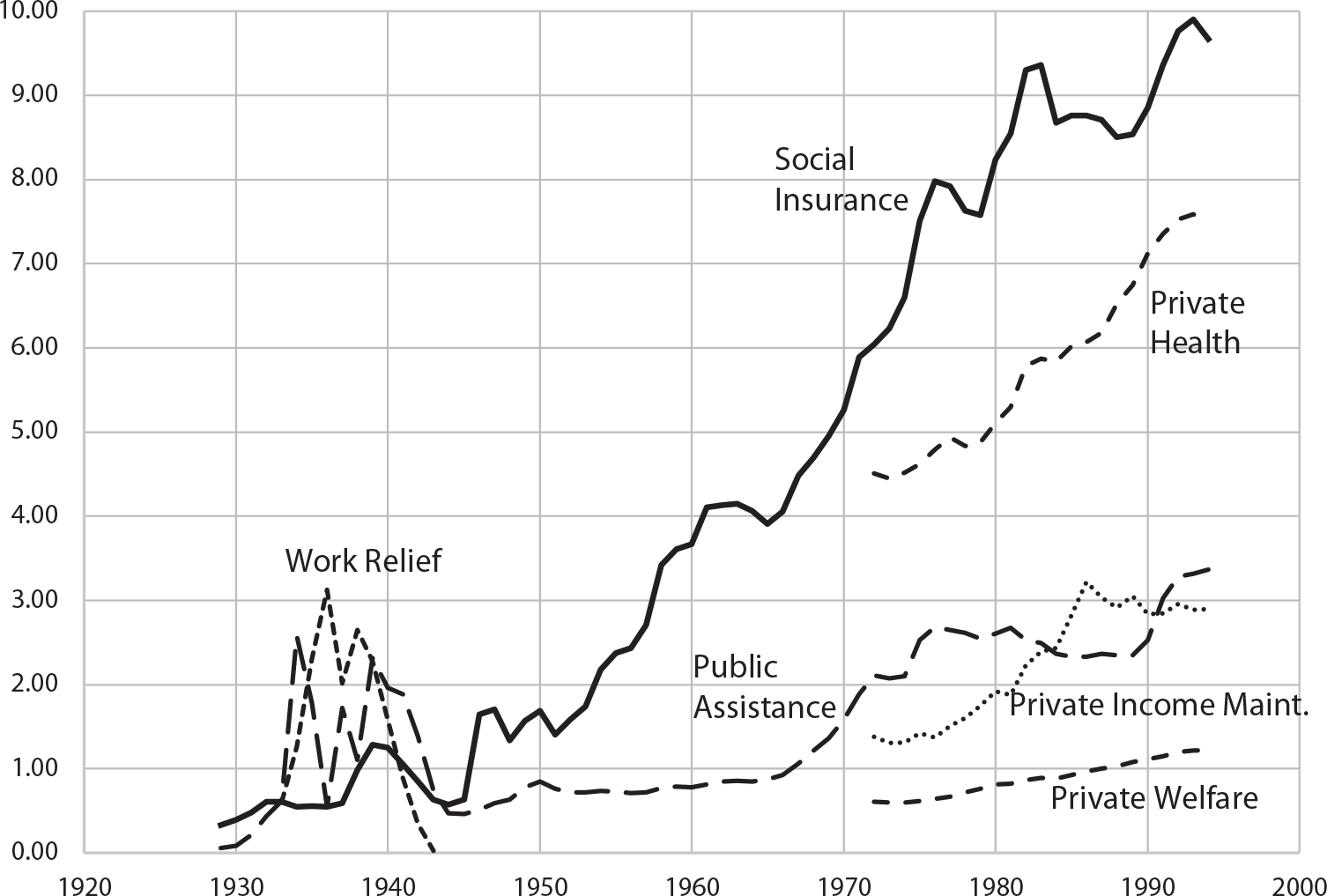
During the twentieth century, total spending on social welfare programs by all government rose from about 1 percent to above 13 percent relative to GDP. This change is often described as the rise of the welfare state. Such a description hides much of the nature of the change. One definition of welfare is public assistance to the poor. As seen in Figure 1, that type of public assistance has never risen above 4 percent of GDP. It rose above 2 percent relative to GDP in the heart of the Great Depression when it was joined by roughly similar shares of work relief payments under the New Deal. After Medicaid was instituted to provide medical care to the poor in 1966, public assistance rose to above 3 percent relative to GDP, in part because more effective medical care led to greater shares of overall medical spending in GDP. Part of the reason for this relatively low amount relative to GDP likely relates to the pure transfer feature of public assistance. Throughout the century, there was support for transfers to people who fell on hard times through no fault of their own, but there were extensive debates about the size of the “undeserving poor” population, whose own decisions led to their demise or who gamed the system (Moffitt Reference Moffitt2015; Katz Reference Katz1989; Patterson Reference Patterson2000). The stigma of being labeled “undeserving” also limited applications for benefits by the eligible poor.
SOCIAL INSURANCE, PUBLIC ASSISTANCE, WORK RELIEF, PRIVATE HEALTH, PRIVATE INCOME MAINTENANCE, AND PRIVATE WELFARE RELATIVE TO GNP, 1929–1994E

The lion’s share of the rise in social welfare spending came in the form of expansions in social insurance. Social insurance relative to gross national product (GNP) rose from less than 1 percent in 1929 to roughly 10 percent by the end of the century. The insurance feature distinguished it from public assistance in several ways. There was no social stigma because the worker could easily claim that she or her employer paid an upfront premium for her benefits. It was not a poverty program because coverage extended to workers and the self-employed throughout the income distribution. Further, the absence of pure transfers made these programs easier to sell to the general taxpayer.
Franklin Roosevelt understood this distinction when he proposed the Social Security Act in 1935. For the elderly, it included both grants for state means-tested Old Age Assistance (OAA) programs for the elderly poor and the Social Security pension program for workers. In his radio address in January 1935, he declared that UI and Social Security would be “self-sustaining” and would not be funded out of general taxation (Roosevelt Reference Roosevelt and Zevin1946, pp. 41–45). The tie between income and pension benefits (although somewhat loose) and the cap on payroll income to be taxed for any employee were set specifically because the Social Security pension program was social insurance. Roosevelt was adamant that the program should be self-funding for a long period. When the Committee on Social Security sent him a draft bill that would have led to a future deficit after 1965, Roosevelt sent it back with the statement: “We can’t sell the United States short in 1980 any more than in 1935.” The Committee thought they had resolved the issue with their final bill, but experience over the next several years led the SSA to switch to the pay-as-you-go system that many countries have adopted (Schieber and Shoven Reference Schieber and Shoven1999, pp. 36–37).
The pay-go system has created funding challenges that have led to increases in the payroll taxes designed to fund it from 2 percent shared equally by worker and employer to 10.7 percent in 1999. Disability Insurance in 1957 and Medicare in 1966 were added to the mix of pay-go programs with specific taxes meant to act like premiums. These funds are not actuarily sound in the sense required for private providers of similar pensions or insurance. Instead, they are funded with government bonds in trust funds. These are essentially government IOUs that promise that the national government will collect enough in taxes to pay the pensions and benefits promised when someone becomes eligible for them. Given the funding method and the relationship between taxes collected and benefits paid, there are cross-subsidies within the programs that benefit lower earners that might be similar to welfare redistribution. Yet, given that all contributors at all income levels get benefits unless they die early, they were structured to look like social insurance programs and not poverty programs.
Unemployment Insurance and WC work more like private insurance. Unemployment Insurance is funded by employers with the federal government paying only administrative costs. Workers’ Compensation requires employers to purchase insurance or provide proof that they have adequate resources to self-insure to cover the medical and wage replacement costs for workplace accidents. Both programs are “experience-rated” because employers who release more workers into unemployment or have more workplace accidents pay higher amounts into the system.
Given the multiple definitions of welfare and that the majority of the rise in funds distributed were in social insurance programs, the public and scholars should really be referring to the rise of the social insurance state in their descriptions of the trends in the United States
INTERNATIONAL COMPARISONS OF SOCIAL WELFARE SPENDING
Modern social welfare programs in the United States operate more as safety nets than in many other high-income countries. While governments provide social insurance and public assistance, a large majority of American households also obtain pensions and health, life, and disability insurance through their employers. Figure 1 shows that private health expenditures rose from 4.5 percent in 1972 to 7.5 percent in 1994 and private income maintenance expenditures rose from 1.4 to 2.9 percent. Meanwhile, private transfers designed to aid the poor rose from 0.6 to 1.2 percent. The U.S. system is often contrasted with more universal government-based systems in high-income democratic countries.Footnote 4 All have market economies, but their governments are more heavily involved in providing health care and in providing funds for child care for all households.
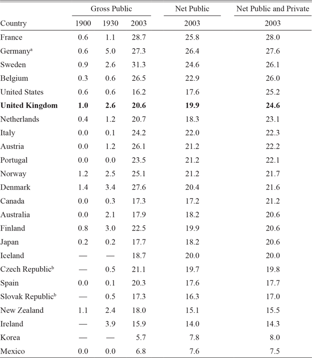
The dramatic rise in social welfare spending internationally in the twentieth century is documented in Table 1. It was less than 2 percent relative to GDP in each of the countries in 1900 and was above 2 percent in only a handful in 1930. By 2003, net public and private social welfare spending—after incorporating public spending, private spending, and public mandates and netting out taxes—in the United States had risen to 25.2 percent relative to GDP, which ranked the United States fifth among the OECD countries in Table 1. How the funds were spent differed greatly, however. Gross public spending typically has been the comparison made in most cross-country comparisons. In 2003, the United States ranked fourth from the bottom in this measure. In 2003, most of the other countries had much higher consumption taxes and the countries with the highest gross public spending tended to tax benefits for welfare recipients. Meanwhile, the United States offered more tax breaks and the Earned Income Tax Credit (EITC) made payments to workers with low enough earnings.Footnote 5 As a result, net public welfare spending as a percentage relative to GDP was substantially lower than the gross spending for most countries, while it was somewhat higher in the United States.
ESTIMATES OF SOCIAL WELFARE EXPENDITURES AS A PERCENTAGE RELATIVE TO GDP IN THE UNITED STATES AND OTHER OECD COUNTRIES, 1900–2003

a Calculated for German Empire in 1900 and 1930.
b Calculated for Czechoslovakia in 1900 and 1930.
Notes: The OECD measures of government social welfare expenditures include old-age pensions, survivor benefits (not from private life insurance), incapacity-related aid, health expenditures, aid to families, unemployment benefits, income maintenance, government job training, and housing subsidies. Gross public is the most widely reported figure. Net public adjusts for taxes paid on benefits, consumption taxes, and tax breaks. Net public and private adds in net private expenditures (mandatory and voluntary). The OECD did not report full information for Switzerland in 2003. Relative to GDP, gross public spending was 1.2 percent in 1930 and 20 percent in 2003, private spending was 8 percent, and no information was provided for net private and public spending.
Sources: The data for 1900 and 1930 come from Lindert (Reference Lindert1994, p. 10). For 2003, the data come from OECD (2007, p. 82).
The United States had dramatically higher private social welfare spending, which raised the U.S. private and net public spending relative to GDP into fifth place on the list. Consider some comparisons with the Nordic countries, which have been strong advocates for universal systems. Private pension payouts in 2003 were 3.8 percent relative to GDP in the United States compared with 2.2 percent in Denmark, 2 percent in Sweden, and less than 1 percent in Finland and Norway. The most obvious difference was in health care spending. In 2003, Americans spent 15.1 percent of GDP on health care, substantially more than in the Nordic countries. The United States spent 6.7 percent relative to GDP through government on the elderly, the poor, and veterans and another 8.4 percent privately on the rest of the population. In comparison, the Nordic countries spent between 5.9 and 8.4 percent of GDP on health care with 1.5–2.1 percent privately.Footnote 6 Among the reasons claimed for higher U.S. health expenditures has been the much higher administrative costs associated with market insurance (Himmelstein et al. Reference Himmelstein, Jun, Busse, Chereul, Geissler, Jeurissen, Thomson, Vinet and Woolhandler2014). Subtract one-third of the private health expenditures for administrative costs, and the private health spending in the United States falls by 2.8 percent of GDP and U.S. private and net public welfare spending falls to 22.4 percent of GDP, which causes the United States to fall only from fifth to eighth, still above many other countries said to be focusing heavily on social welfare spending.Footnote 7
FIFTY-ONE OR MORE SOCIAL WELFARE SYSTEMS IN THE UNITED STATES
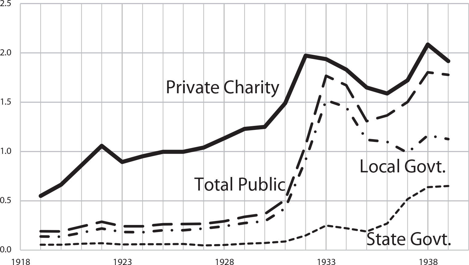
Throughout the twentieth century, the United States had at least 51 different welfare systems, more if local government and charity programs are included. The variety is the legacy of a history of the organization of poverty programs in the United States. Prior to 1910, local governments and charities played the dominant role in providing public assistance for nonveterans with outdoor relief, almshouses, and hospitals.Footnote 8 Local governments and private charities continued to provide a large share of the social welfare spending into the 1930s. For example, the Massachusetts Department of Public Welfare collected probably the most comprehensive records on private and public spending during the period, and Figure 2 shows some summary information compiled by Livingston (Reference Livingston2011) from the Massachusetts Board of Charity (1900–1919) and the Massachusetts Department of Public Welfare (1920–1930). Local government social welfare spending rose from about 0.25 percent of personal income in Massachusetts in 1919 to nearly 2 percent in 1940, while private charity rose from around 0.5 percent to around 2 percent in 1933. Massachusetts has been considered a relatively progressive state, so these figures are likely higher than for the United States as a whole. Even so, the scattered information I have seen suggests to me that the very low figure for public assistance in 1929 in Figure 1 understates the true level. More quantitative research on this period will be valuable.
STATE, LOCAL, AND PRIVATE WELFARE SPENDING AS A PERCENTAGE RELATIVE TO PERSONAL INCOME IN MASSACHUSETTS, 1919–1940

In 1911, state governments began adopting Mothers’ Pensions (MPs) to provide funds for widows with children and social insurance for workplace accident victims in the form of WC. By 1934, in the heart of the Depression, all but 2 states had MPs, all but 4 had WC, 30 had need-based old-age assistance, 28 offered aid to the blind (AB), and Wisconsin had begun collecting revenues to fund unemployment insurance payments (Fishback and Thomasson Reference Fishback, Thomasson and Carter2006, p. 2-709). Governments at all levels had tried to increase road building and other public works in the early 1930s. In response to the Great Depression, in 1932, the Reconstruction Finance Corporation under President Hoover made $300 million in loans to cities and states for public assistance that were later forgiven. The federal government began playing an active role in public assistance in 1933 with direct and work relief grants from the Federal Emergency Relief Administration to the states, the Civil Works Administration, and the Civilian Conservation Corps program. These and programs such as the Works Progress Administration had ended by 1943. The beginning of the long-term role of the national government in public assistance and social insurance for the general public started with the Social Security Act of 1935, which is discussed more below.
Target Benefit Levels for Households on Public Assistance
State governments determined benefit levels in many public assistance and social insurance programs. As a result, the benefit levels varied a great deal across space and time. The public assistance programs for the elderly and family recipients of aid ran on a budget-deficit principle that established a target level of income and sought to fill the gap between the target and the earnings of the family (Moffitt Reference Moffitt1992, Reference Moffitt and Moffitt2003). These targets show the dollar value of the standard of living that the states sought to ensure for the people they supported. Average spending per recipient cannot provide this information because it is a measure of the average gap between the target and the average pre-transfer incomes of the recipients. In 1911, state governments started enacting MP laws to provide monthly payments to widows with children to allow them to live in their own home rather than be in almshouses (Moehling Reference Moehling2006, Reference Moehling2007) By 1934, all but two states offered MPs and some states had expanded their programs to include mothers who had lost husbands for other reasons. The Social Security Act of 1935 started Aid to Dependent Children (ADC). The national government offered matching grants up to a fixed amount per month for recipients; the states were required to pass enabling legislation to set up a program in each county of the state with specific administrative guidelines, while states retained control over the benefit levels. In 1962, the program was superseded by Aid to Families with Dependent Children (AFDC) when coverage was expanded to include adults caring for dependent children. Welfare reform in 1997 replaced AFDC with TANF, which shifted to block grants away from matching grants to the states and focused more heavily on ensuring that adults in the families returned to work earlier. For ease of exposition, I will use the term “family targets” to refer to target incomes under these programs.Footnote 9
In the 1920s, a handful of states legislated OAA programs for the poor elderly to allow them to live on their own. These early laws typically gave counties the ability to run programs, but the state government allotted no funds. By 1934, 30 states and territories had programs and most were providing state funding, but the amounts paid out often fell well short of target benefits.Footnote 10 As with ADC, the Social Security Act of 1935 began providing matching grants for OAA benefits that were determined by the states. This was the means-tested poverty program for the elderly that complemented the Old Age Survivors’ Insurance (OASI) pension program that is commonly referred to as Social Security. In 1972, the OAA programs were superseded by SSI, in which the federal government set a nationwide benefit level. Benefit levels still varied across states because a number of states added their own payments.Footnote 11 For ease of exposition, I will refer to these benefits for the elderly poor as “elderly targets.”
Over the course of the century, the national government has funded additional poverty programs to supplement, and in some cases to replace, part of the benefits. A school lunch program was started in 1946. School breakfasts and meals during the summer were added in the 1960s. After experimenting with food stamp programs, the national government enacted a more permanent Food Stamp program in 1964. The Agriculture and Consumer Protection Act of 1973 (Public Law 93-86, 10 August 1973) required states to provide the program in all jurisdictions by 1 July 1974. In 1974, the national government set up the permanent Woman, Infants, and Children (WIC) program to provide grants to states to fund better nutrition for poor women during pregnancy and while they raise small children. The national government provided funds for medical vendor payments for ADC and OAA recipients in 1951 (Thomasson Reference Thomasson2002). These were replaced by the Medicaid program in 1966. The Low Income Household Energy Assistance Programs (LIHEAP) began providing funds to cover heating and cooling costs in 1981 (Fishback and Thomasson Reference Fishback, Thomasson and Carter2006, p. 2-696).
My goal is to provide an estimate of the target income that each state established for a family in poverty and an adult aged 65 and over living on their own in 1919, 1926, 1934, 1940, 1958/1960, 1971, 1983, 1990, and 2000. The choice of year and the size of family for the public assistance estimates of the target level living are based on availability of information on target income levels and on cross-sectional cost-of-living comparisons.
For both the old-age and family target benefits, I assume the household starts with zero income so they would receive the full payment, which reflects the target level of income. The three-person family was a mother, a child under school age, and a child of school age; a four-person family has another child in school. The elderly person is assumed to have never worked and, thus, is not eligible for Social Security pensions, Medicare, or Disability Insurance. After 1982, the Green Book, put together by the Department of Health, Education, and Welfare, reported maximum totals for the combination of food stamps and family benefits and for the combination of food stamps and elderly benefits (U.S. House of Representatives, Committee on Ways and Means, various years). In 1971, the states reported maximums for family and elderly benefits alone. In 1971, I added the national average of food stamps per OAA recipient and food stamps per ADC recipient to avoid variation across states in such payments that might have been based on differences in poverty levels. For the school meal programs, I calculated a cost per meal, usually with national information, and assumed that the child ate breakfast and lunch at school for 20 days a month for nine months and ate one summer meal for 20 days a month for three months. The average payment per recipient for WIC was added for the child under school age. LIHEAP benefits were based on state averages of payments per household receiving benefits for both the elderly poor and the family poor.
Medicaid reported the amount paid and the number of recipients for OAA/SSI participants and separately for child and adult recipients of AFDC/TANF, so I reported the amount per recipient in those categories in 1983, 1990, and 2000. For 1971, I only had state estimates for Medicaid for 1970 and 1972, so I used national estimates to interpolate a 1971 value for each state. In 1960, the estimates for the elderly are medical vendor payments for OAA for the year divided by number of OAA recipients in June 1960. For family benefits, I used medical vendor payments for OAA for the year divided by the number of ADC families in June 1960. The ADC benefits target I found was for 1958, and I used the 1960 value for the medical benefits for the total payouts.
I have not included the value of several other programs offered to people in poverty: education, training, childcare, and housing subsidies. The most prominent of these omissions are the rental vouchers and subsidies provided by the U.S. Department of Housing and Urban Development. These were designed to ensure that low-income people paid no more than 30 percent of their income in rent. I do not include them because funding has been limited from the beginning and there were long waiting lists to obtain assistance. For example, in 2019, roughly “3 out of 4 eligible low-income renter households do not receive federal rental assistance.”Footnote 12 Since the benefits were not delivered to the majority of eligible households, they cannot be treated as part of the target. The poor and elderly recipients of rent subsidies received a significant boost to their resources. The ratio of the average nominal annual rental subsidies per unit under Department of Housing and Urban Development (HUD) Section 8 to the poverty line for one elderly person was 0.59 in 1983, 0.67 in 1990, and 0.61 in 2000, and the ratio to the three-person family poverty line was 0.35 in 1983, 0.41 in 1990, and 0.36 in 2000.Footnote 13
Social Insurance Weekly Maximums
Workers’ Compensation and UI are social insurance programs that mandate that the employer provide aid to workers injured on the job and unemployed workers, respectively. Unlike the focus on minimum levels of living for public assistance, the focus for the social insurance programs is on the maximum benefits. The reason is that the states themselves have set the weekly maximums because they wanted to limit their budgets and not pay large amounts to highly paid workers when injured. The weekly maximums were also set to help reduce problems with moral hazard, when workers take more risks given better protection against those specific risks.
Beginning in 1911, Worker’s Compensation laws replaced negligence liability for workplace accidents with a form of strict liability that provides medical treatments and partial replacement of lost earnings. The last state to adopt was Mississippi in 1948. The states have maintained control of WC from its beginnings through to the present. The laws typically included a list of injuries and the length of time that the injured worker or the family of a fatally injured worker is expected to be paid benefits. They also specified the share of earnings to be replaced. A large share of states replaced up to two-thirds of lost earnings with nontaxable payments, but they also established maximum weekly payments that have tended to be binding for a large share of workers (Fishback and Kantor Reference Fishback and Kantor2000). In the 1970s, after a National Commission on State Workmen’s Compensation Laws described a broad range of problems with WC, most states indexed their maximums to average weekly earnings in the state (Allen Reference Allen2015). Over the course of the century, the laws have expanded coverage to include some form of workplace-related illnesses. States or state courts administered the programs and set the benefits, but WC could also be described as a mandate that the employer purchase insurance or document his ability to pay the proper benefits in a form of self-insurance. I did not include in the weekly maximum benefits the coverage of medical costs related to the workplace injury or disease because the coverage is specific to the injury and does not include coverage for other health issues.
In the early 1930s, a number of states explored the possibility of providing benefits to unemployed workers. Wisconsin had already started to build up its reserve fund when the Social Security Act of 1935 created a set of administrative rules and subsidies for states to adopt UI. Employers paid into a reserve fund, which was paid out to unemployed workers. The states chose the income replacement rate (often 50 percent), a weekly maximum payment, and the number of weeks of payments. During some recessions, the number of weeks increased with subsidies from the national government. Like WC, UI has the flavor of a government mandate because the employers pay for the full costs of benefits. The only role played by governments was to administer the funds; the national government covered the cost of administration.
INCOME STANDARDS USED FOR COMPARISONS WITH TARGET BENEFITS
In the “Rhetoric of Economics,” McCloskey (Reference McCloskey1983) made the important point that a number by itself is of little use until it is compared with others. How did the state targets compare with measures of poverty and earnings opportunities? Various authors and government agencies have offered estimates of poverty lines and living standards, but they often cover only a handful of years.Footnote 14 For comparison with the targets, I chose three income standards that have been consistently measured in essentially the same way throughout the century. These include the national poverty line, average earnings plus benefits for manufacturing production workers in the state, and state per capita incomes.Footnote 15
The official national government poverty line is used by governments as a basis for determining eligibility for benefits and seems to have been a target minimum level for household income for many governments. In 1963, Molly Orshansky of the SSA used a U.S. Department of Agriculture measure of economy-plan food budgets and multipliers based on ratios of food spending to after-tax income to develop a measure of an “inadequate” budget. Officials associated with the War on Poverty used Orshansky’s measures as their poverty line. By the late 1960s, it became clear that the multipliers were becoming outdated and federal officials then indexed the poverty line to the Consumer Price Index (CPI).Footnote 16 To extend the poverty line back to earlier years, I used a poverty line based on work by Ornati (Reference Ornati1966), who calculated his measures in a way similar to Orshanksy’s method.Footnote 17 The poverty lines used match the household sizes of one elderly person over 65 and three or four persons for the family group. The UI and WC benefits are compared with the four-person family poverty line.
A second income standard is the weekly earnings plus public and private benefits paid by employers to manufacturing production workers in each state. People on public assistance tended to have less education; therefore, working in manufacturing positions that required less education often was one of their best paths to greater prosperity. Manufacturing earnings and benefits are natural comparisons for WC and UI benefits because many of the workers receiving benefits came from that sector. The BLS reported consistent series by state on average weekly manufacturing earnings of production workers, which included overtime pay from 1939 through 2000. For 1934, I used weekly earnings reported by the Bureau of Labor Statistics (1934) in their Trend of Employment reports. For 1926 and 1919, I used estimates of weekly earnings by state that Fishback and Kantor (Reference Fishback and Kantor2000, Reference Fishback and Kantor2018) interpolated from national average weekly earnings using state annual earnings per worker.
Employers shared the cost of a variety of private benefits for workers, including life insurance, disability insurance, pensions, and paid leave. In addition, they paid a share of the costs of public benefits, including Social Security, Medicare, Disability Insurance, UI, and WC. These benefits are included as part of the income standard because they were part of the pay package for production workers and they were absent in the target benefits paid to public assistance recipients. The availability of benefits to injured and unemployed workers also varied across employers. I could not get estimates of state level figures for these benefits. As a result, I used national data on employer compensation cost for production and related workers from Sundstrom (2006, p. 2-322) and national data on supplements to wages and salaries developed by Lebergott and reported in U.S. Census Bureau (1975, pp. 166, 174) to create ratios to earnings that were then multiplied by weekly earnings in each state.Footnote 18 The benefit share of the employment package probably varied across states. In states where the benefits were a smaller share, the earnings and benefits package is overstated, which understates the ratio of the public assistance and social insurance targets to the employment package in manufacturing.
The final income standard is state per capita personal incomes from the Bureau of Economic Analysis (2008) and Martin (Reference Martin1939) times the household number of recipients: one for the elderly, three or four for the family, and four for UI and WC. Per capita income is a common metric for comparisons of well-being and it includes incomes from all sectors of the economy. One caveat, personal income includes public assistance and social insurance transfers and the population includes the transfer recipients; therefore, per capita income will understate the incomes of nonrecipients.
TARGET BENEFITS IN 2019 DOLLARS AND RELATIVE TO INCOME STANDARDS
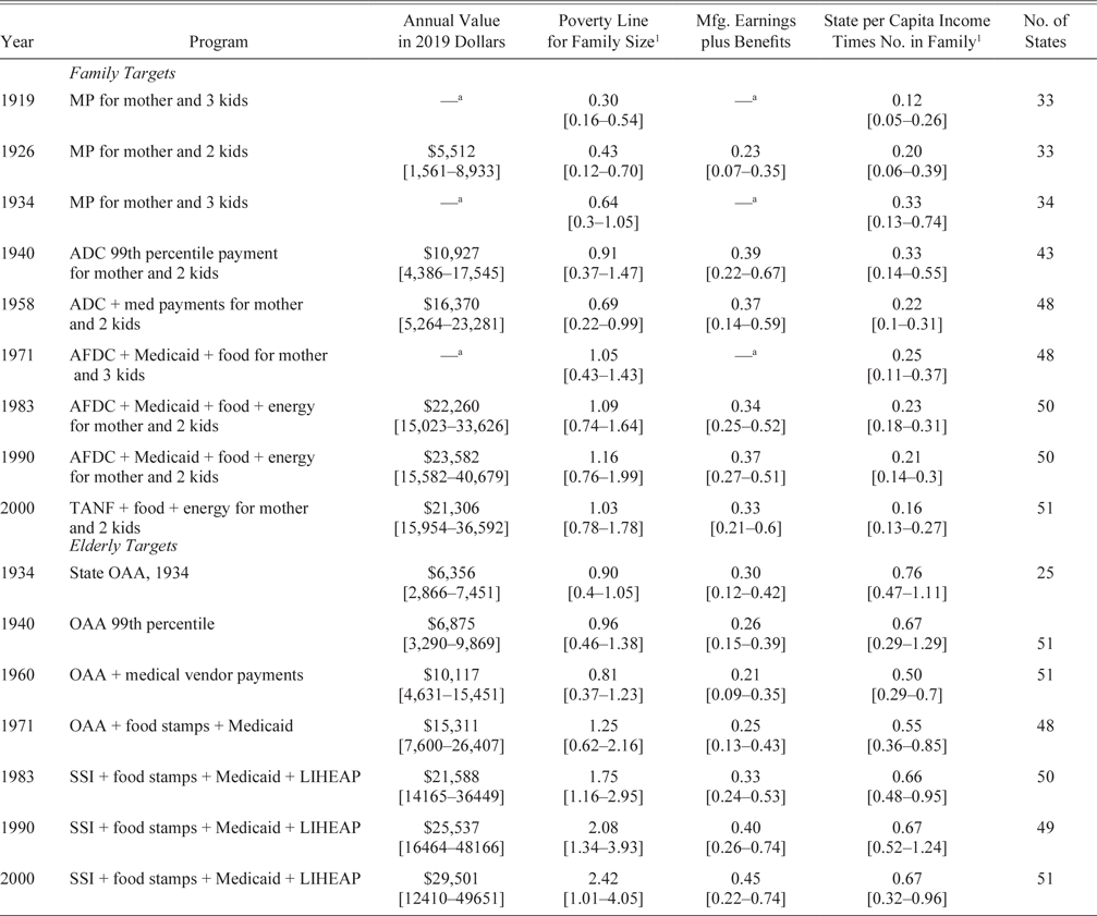
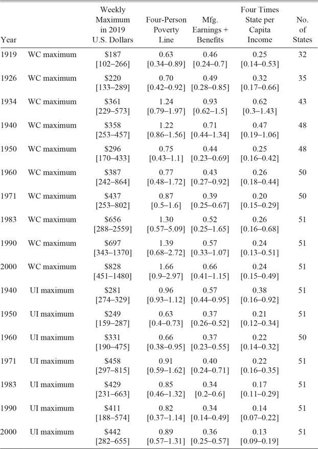
Over the course of the century, the real value of national mean benefits in 2019 dollars in Tables 2–4 rose substantially in each of the four social welfare categories.Footnote 19 The national Urban CPI from the BLS is used to adjust for inflation in all states, and the means are calculated using state populations as weights. The elderly public assistance targets were the only ones to rise continuously throughout. Increases in average medical benefits were a primary contributor. The target for three-person families rose continuously to 1990 but was lower in 2000 after the TANF reforms in 1997. The real weekly maximums for WC and UI both fell during the 1940s war decade. After 1950, WC maximums continued to rise each decade, while UI maximums rose between 1950 and 1971, stayed roughly the same for two decades, and then rose again in the 1990s.
POPULATION-WEIGHTED MEANS OF TARGET VALUES IN 2019 DOLLARS AND RATIOS OF FAMILY AND ELDERLY TARGET BENEFITS TO THREE INCOME STANDARDS, MINIMUMS AND MAXIMUMS IN BRACKETS BELOW

1 Per capita income is multiplied by 3 for 3-person families and 4 for 4-person families.
a To facilitate comparisons over time, value is not reported because the family size is larger. Reported values relative to poverty line because the poverty line was adjusted for family size.
Source: See the Online Data Source Appendix.
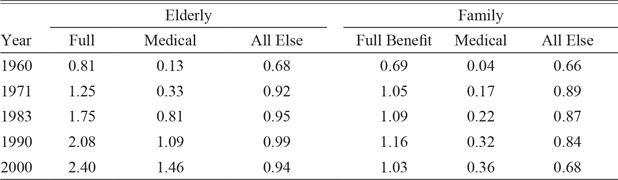
POPULATION-WEIGHTED MEAN RATIOS OF BENEFITS TO APPROPRIATE POVERTY LINE: ALL BENEFITS, MEDICAL BENEFITS, AND ALL ELSE, 1960–2000

Notes: WC is Workers’ Compensation and UI is Unemployment Insurance.
Source: See the Online Data Source Appendix.
POPULATION-WEIGHTED MEANS OF WEEKLY MAXIMUMS IN 2019 DOLLARS AND RATIOS OF WORKERS’ COMPENSATION AND UNEMPLOYMENT INSURANCE WEEKLY MAXIMUMS TO INCOME STANDARDS, MINIMUM AND MAXIMUM IN BRACKETS BELOW

Notes: WC is Workers’ Compensation and UI is Unemployment Insurance.
Source: See the Online Data Source Appendix.
The enormous variation across states is shown by the minimums and maximums reported in brackets below the means. In all but three of the comparisons in Tables 2 and 4, the maximum is more than two times as large as the minimum, and in more than half of the comparisons, the maximum is more than three times the minimum. In comparisons over time, the minimums in 2000 were lower than the mean values circa 1960 for the family, elderly, and UI targets and circa 1970 for WC.
Tables 2–4 also contain ratios of the targets to the income standards. The ratios to the poverty line reflect a comparison between the state benefit target and a single national poverty standard that does not take into account differences across states in cost of living and earning opportunities. The other two standards vary across states in each year; therefore, the ratios to the manufacturing and per capita income standards compare the target benefit in that state to the types of opportunities available within the same state.
Family Benefits Relative to Income Standards
During the MP era when only state and local governments funded the benefits, MP benefits relative to the poverty line in states with maximums in Table 2 rose from 30 percent of the poverty line in 1919 to 64 percent of the poverty line in 1934. The Social Security Act of 1935 introduced federal matching grants to the states, and states continued to raise benefits relative to the poverty line. Over the next two decades, the state legislatures did not raise benefits to keep pace with the poverty line, manufacturing earnings, and benefits or per capita incomes.Footnote 20 When the AFDC reform in 1962 expanded coverage to adults caring for dependent children, family benefits rose to 105 percent of the poverty line in 1971 and continued to rise to 116 percent of the poverty line in 1990. A big part of the rise between 1958 and 1990 came in the form of medical benefits; the ratio of medical benefits to the poverty line rose from 0.04 in 1958 to 0.32 in 1990 in Table 3. In 1997, the TANF reforms that emphasized a return to work caused benefits to fall in real dollars and relative to all three of the income standards. Between 1990 and 2000, nonmedical benefits relative to the poverty line in Table 3 fell from 84 percent of the poverty line in 1990 to 68 percent in 2000.
Ziliak (Reference Ziliak2002, p. 500), who joined Hannon in editing the section of the Historical Statistics of the United States on poverty programs prior to 1900 (Ziliak and Hannon 2006), stated that the ratio of poverty benefits to common laborers’ wages had stayed relatively constant during the twentieth century at around 0.3. He was referring to average payments to recipients, while the measure here is the target standard of living. We are also referring to different wage measures. Yet, it is still worthwhile to see if there is a ratio that has held relatively constant over time.
In the comparisons to manufacturing benefits and earnings and to per capita incomes, the ratio is the benefit target to the income standard in the same state. When Ziliak made his statement, he was not considering the full value of the manufacturing employment package, but after 1926, his declaration of a rough constant ratio is not too far off for the national averages. The national average ratio of the family targets to manufacturing benefits and earnings ranged between 0.34 and 0.39 between 1940 and 1990, before falling back to 0.33 after the TANF reform. In the comparison of targets to per capita personal incomes, the ratio bounced around between 0.12 and 0.33 before World War II but held steady between 0.21 and 0.25 from 1958 to 1990 before the TANF reforms caused it to drop to 0.16 in 2000.
Elderly Benefits
American governments have treated the elderly poor better than they have treated poor families with children. The states in Table 2 that had old-age assistance programs in 1934 had mean national target levels of 90 percent of the poverty line, compared with 64 percent for families. They fared even better after 1970 with targets that rose from 125 to 242 percent of the poverty line, while family benefits ranged between 103 and 116 percent of the poverty line. The national average of the elderly target has risen faster than manufacturing earnings and benefits and held steady at about two-thirds of per capita incomes between 1983 and 2000.
A small part of the difference between the poverty line ratios for the elderly and the family targets after 1960 is due to the elderly receiving higher nonmedical payments of 0.92–0.99 of the poverty line in Table 3 compared with 0.68–0.89 for families. Most of the difference comes from a much sharper rise in medical payments for the elderly poor than for the poor families. Elderly medical benefits as a share of the poverty line in Table 3 rose from 0.13 in 1960 to 1.46 in 2000, much faster than the rise from 0.04 in 1958 to 0.36 in 2000 for the family medical benefits. Between 1971 and 2000, the elderly Medicaid payments per recipient in Table 3 also rose much faster than the rise in payments per recipient in the general Medicare program, which rose from 0.18 to 1.01 of the poverty line (Centers for Medicare and Medicaid 2002, pp. 103, 117).
WC and UI Weekly Maximums
In 1919 and 1926, WC benefits in Table 4 were 63 and 73 percent of the four-person poverty line. They rose to 124 percent of the poverty line by 1934, as about half of the rise was due to rising benefits and half due to falling incomes in the Depression. Between 1940 and 1960, state governments were slow to increase weekly maximums and to keep pace with rising wages and incomes; therefore, the benefits fell back to 75 percent of the poverty line (Allen Reference Allen2015). The reforms of the 1970s led to an increase in benefits by 1983, and the indexing of benefits to state average earnings kept them rising to 166 percent of the poverty line in 2000. Relative to the manufacturing employment package, the national average ratio rose from 0.39 in 1971 to 0.66 in 2000. Between 1950 and 2000, the national ratio to a household with four times per capita personal income bounced around between 0.21 and 0.26.
As was the case for WC, states were slow to increase UI benefits during the war decade of the 1940s and the national average ratio of weekly maximums to the four-person poverty line in Table 4 fell from 0.95 to 0.63. The states caught up and the national average benefit ratio rose to 0.91 of the poverty line in 1971 but only ranged between 0.82 and 0.89 afterward. Since 1950, the national average UI benefit ratios to manufacturing employment packages have ranged from about 0.34 to 0.4. The UI maximum ratio to the income of a family with four times the state per capita income was around 0.22 from 1950 to 1970 but fell to around 0.13 in 2000. The difference in trends between UI and WC likely relates to differences in the number of states that automatically index their maximums to weekly wages. By 2000, 43 states were indexing their WC benefits, while as late as 2015, only 33 states indexed unemployment insurance benefits (Allen Reference Allen2004, p. 43; U.S. Department of Labor, Employment and Training Administration 2015, pp. 3-13–3-14).
THE IMPACT OF CROSS-AREA COST-OF-LIVING ADJUSTMENTS
Most panel studies of income, earnings, and public benefits in the twentieth century, including my own, adjust for national inflation but do not directly adjust for cross-sectional differences in the cost of living. One reason for the lack of adjustment is that studies by the BLS and the Works Progress Administration that compared the same basket of goods and services across areas covered only about half the years between 1935 and 1982 with a changing cast of cities. The situation is better after 1982 because Carrillo, Early, and Olsen (2014a, 2014b) developed a nationwide panel dataset of costs of living. All of these studies show substantial cross-sectional differences in the cost of living across cities throughout the century and states after 1982.Footnote 21 In estimations of relationships between these variables and other factors, the consequences of failing to adjust might not have been severe because scholars used area fixed effects to control for the unchanging components of area differences. Lack of adjustment is much more of a problem when comparing the integration of labor markets and the adequacy of the level of living of earnings and benefits, particularly when comparisons are made with a national standard such as the poverty line.
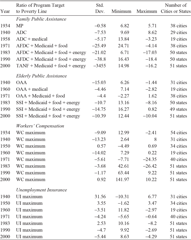
The consequences of making cost-of-living adjustments for the ratio of targets to the poverty line are shown in Table 5 and Figures 3 and 4. The targets and poverty lines are indexed to living costs in Boston in the same year because Boston appeared in all of the cost-of-living studies.Footnote 22 Because the values are deflated by Boston prices, the population-weighted means of the targets to the poverty line change; therefore, in Table 5, I compare the ratios of the standard deviation to the mean, the minimum to the mean, and the maximum to the mean before and after the cost-of-living adjustment.
PERCENTAGE CHANGE IN SUMMARY STATISTICS RELATIVE TO THE MEAN WHEN ADJUSTED FOR CROSS-SECTIONAL DIFFERENCES IN COSTS OF LIVING: DIFFERENT PROGRAMS RELATIVE TO THE POVERTY LINE

Notes: The summary statistics were calculated using population weights for program years both before and after adjusting for cross-sectional differences in the cost of living. The population-weighted means differed somewhat before and after the adjustments in each program year. To put the summary statistics on the same basis when comparing the adjusted and unadjusted measures, the standard deviation, minimum, and maximum are divided by the mean for that year and program. Then the percentage difference between the adjusted and unadjusted ratios to the mean is calculated. Cost-of-living comparisons are available only for cities before 1983 and for cities and states (plus Washington, DC) thereafter.
Sources: For the sources of underlying data, see the Online Data Source Appendix.
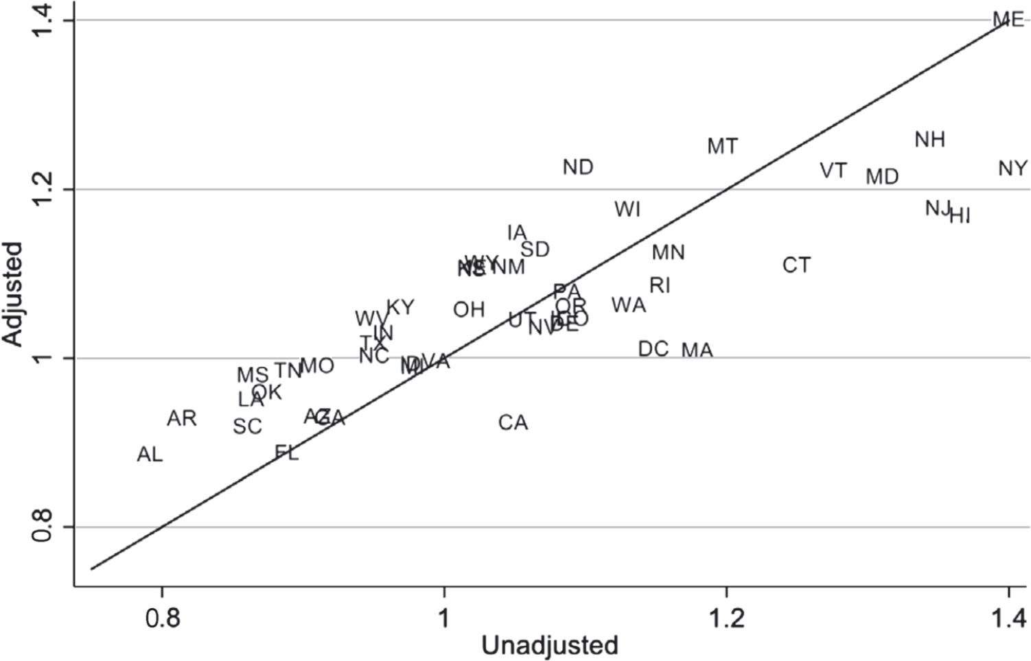
COMPARISONS OF THE RATIO OF FAMILY BENEFITS TO THE POVERTY LINE IN 2000 WITH AND WITHOUT ADJUSTING FOR CROSS-STATE DIFFERENCES IN THE COST OF LIVING

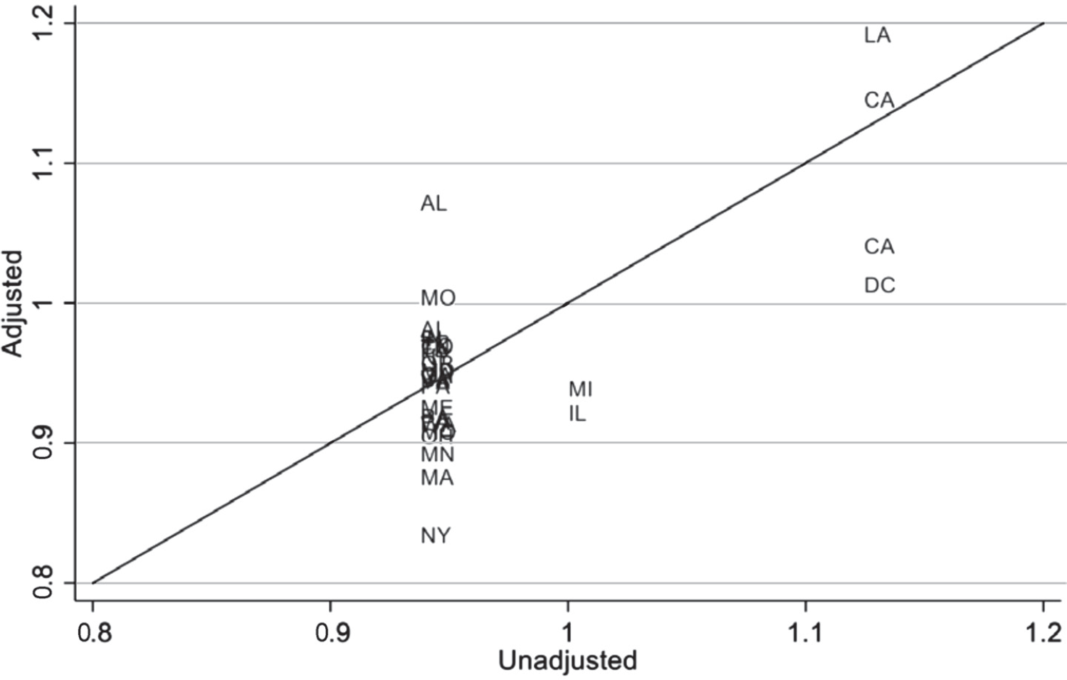
COMPARISONS OF THE RATIO OF UNEMPLOYMENT INSURANCE MAXIMUM TO THE POVERTY LINE FOR A FOUR-PERSON FAMILY IN 1940 WITH AND WITHOUT ADJUSTING FOR CROSS-CITY DIFFERENCES IN THE COST OF LIVING

The adjustments lead to substantial changes in cross-sectional comparisons of benefits. The family target ratios to the poverty line change dramatically in Figure 3. Remember that the poverty line is the same for all states in Figure 3, so the adjusted benefits are comparisons of the purchasing power of the family target benefits. The purchasing power of benefits in Alaska, Hawaii, Massachusetts, New Jersey, New York, Washington, DC, and California (all in the lower right) after adjustment are all at least 10 percent lower than before, while the purchasing power in 14 states at the upper left rose by more than 10 percent. Massachusetts’ benefit ranking fell from 11th to 35th, California’s from 27th to 48th, and Washington, DC’s from 14th to 34th. At the other end, North Dakota moved up from 17th to 5th and Iowa rose from 26th to 12th. Even after adjustments, however, states in the deep South still remained near the bottom of the rankings.
The benefit target ratios do not change as dramatically in all years or for other benefit targets. The comparisons in Table 5 show that the cost-of-living adjustments reduced the standard deviation and increased the minimum in nearly every period. In roughly half of the comparisons, the maximum was lowered as well. These patterns typically happen when the states choose a broad range of benefits.
There are a handful of situations in Table 5 where the standard deviation increases after cost-of-living adjustments. The UI benefit ratios in 1940 in Figure 4 illustrate that this happened when many states chose the same unadjusted benefit levels. In 25 of the 31 observations, the state chose a weekly maximum of $15 per week; therefore, the adjustments raised the UI/poverty line ratio in Birmingham, Alabama from 0.93 to around 1.07, while the ratios for New York City and Washington, DC fell to around 0.83. It is likely that the same situation was present when states often chose the same maximums when introducing WC and MPs between 1911 and 1915. This kind of pattern always happened when a single national benefit was paid, causing the purchasing power of the national benefit to be much higher in southern states than in the remaining states. As one example, purchasing power in Arkansas in 2000 was 42 percent higher than it was in Boston (Carrillo, Early, and Olsen 2014b).
Adjusting for cost-of-living differences also reduces the correlations between the benefits of the programs across states within the same year. For example, one might expect high positive correlations between programs because states with high WC maximums would also have higher UI maximums and higher elderly and family benefits. Without adjusting for costs of living, the correlation across states in 2000 between family TANF benefits and elderly SSI benefits was 0.56. After adjusting for cost of living, however, the correlation fell to 0.39. The drop from cost-of-living adjustment is even stronger for other comparisons in 2000. The correlation between TANF and UI benefits falls from 0.34 to –0.02, and between TANF and WC, benefits fall from 0.35 to 0.11. Similar drops from cost-of-living adjustments occur as well for 1990 and 1983.
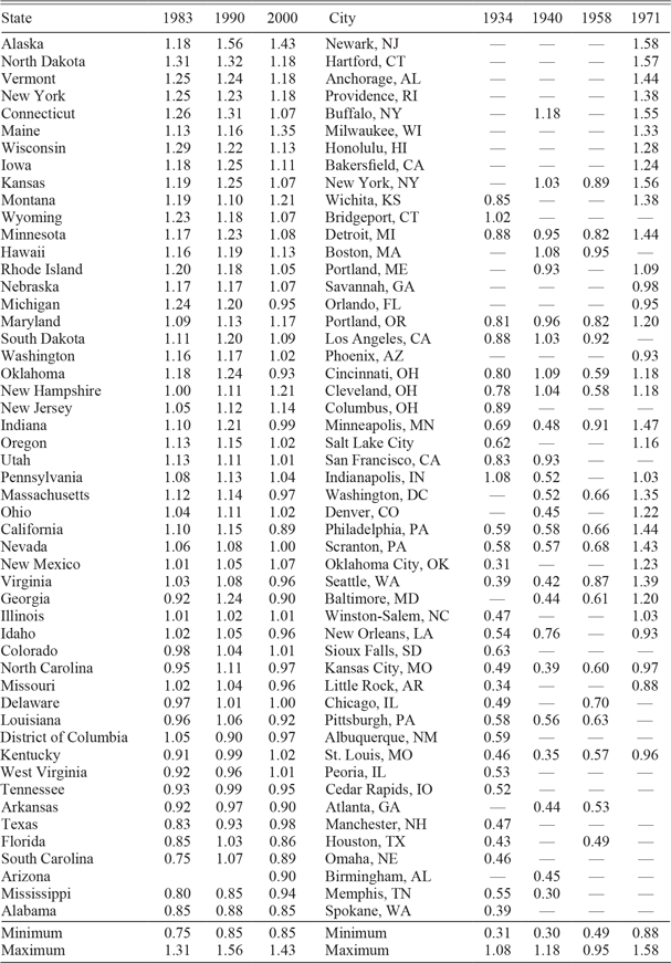
Having shown that cross-sectional adjustments can have substantial impact on the relative purchasing power of benefits and on correlations, I added Table 6 to show the ratios to the national poverty line of family benefits after adjusting for the cost of living across states for 1983–2000 and across cities for 1934–1971. The lists are ranked by the averages for states and cities for their respective time period. See the dataset and data descriptions posted online to accompany the article for other benefit targets. In panel regressions of the ratios with state and year fixed effects and a variety of political and economic correlates, the coefficients of the state fixed effects were the only ones that were statistically significant. Therefore, it appears that the unchanging features of the state political and economic environments drive the differences across areas. After adjusting for cost of living, Hawaii, Alaska, and cities and states in the Northeast, Midwest, and Plains tended to rank at the top of the distribution and most states in the bottom were in the South.
RATIO OF FAMILY BENEFITS TO POVERTY LINE AFTER ADJUSTING FOR CROSS-SECTIONAL DIFFERENCES IN COST OF LIVING, CITIES 1934–1971 AND STATES 1983–2000

Sources: State listings are sorted by the average of the ratios for 1983–2000. City listings are sorted by the average of the ratios for 1934–1971. Data for cost-of-living adjustments are from Carrillo, Early, and Olsen (2014a, 2014b), Lamale and Stotz (Reference Lamale and Stotz1960), Ruiz (Reference Ruiz1972), U.S. Bureau of Labor Statistics (1951), Stecker (Reference Stecker1937), and Anonymous (1940).
EFFECTS ON POVERTY
The rise in benefits along with the reduction in tax rates for lower incomes and the introduction of the EITC contributed to a sharp reduction in poverty rates between the 1960s and the end of the century. Meyer and Sullivan (Reference Meyer and Sullivan2013) show that the official income poverty rate prior to taxes and transfers fell from around 19 percent of the population in 1963 to 11 percent by 1973 and then bounced upward to 15 percent in the early 1990s before falling to 11 percent in 2000. After adjusting for taxes and the types of transfers described here, as well as Social Security pensions, the poverty rate fell from over 31 percent in 1963 to around 7 percent in 2000. After adjusting for taxes and transfers, the ratio of income after taxes and transfers for the 10th percentile to the 50th percentile fell from around 0.43 in the late 1970s to 0.37 in the early 1980s and held steady at around 0.4 for the rest of the century (Meyer and Sullivan Reference Meyer and Sullivan2017).Footnote 23
Maintaining consumption during periods of income decline also was a major target of public assistance programs. Meyer and Sullivan (Reference Meyer and Sullivan2013) show that the percentage of households with consumption levels of less than 50 percent of the median income rose from around 10–11 percent around 1960 to 13 percent in 1985 and then fell to below 11 percent in the late 1990s. By 2010, the share had fallen below 10 percent. Meanwhile, the ratio of consumption at the 10th to consumption at the 50th percentile was around 0.53 in the early 1970s, fell to around 0.50 in 1984, and then stayed steady at 0.5 through 1999. Between 2000 and 2014, it fluctuated between 0.5 and 0.53 (Meyer and Sullivan Reference Meyer and Sullivan2017).
BENEFIT COMPARISONS TO PER CAPITA GDP IN OTHER COUNTRIES
Historically, the United States has been among the richest countries in the world in comparisons of income per capita after adjusting for purchasing power parity. The comparisons are for average incomes and do not reflect how the poor are treated in each country. The calculations made here offer an opportunity to at least compare the target benefit levels for the poor, injured, and unemployed in the United States to the average incomes in other countries. The Maddison Project at Utrecht University provides estimates of per capita income in many countries converted to 2011 U.S. dollars in purchasing power parity. I adjusted the population-weighted mean target benefits to 2011 U.S. dollars using the CPI.
Without further adjustment, this measure will bias the rankings against the benefits in the United States because the U.S. benefits will not include the value of government-provided education, military defense, and other quasi-public goods provided by governments that would be included in the per capita GDPs. To reduce this bias, I adjusted the benefits by multiplying them by the ratio (C + G)/C, in which C is personal consumption expenditures and G is government spending after subtracting government payments for public welfare, health care, veterans, housing, and social insurance.Footnote 24 The subtraction is designed to take out any transfer payments that might go to the poor, injured, or unemployed. After multiplying the (C + G)/C ratio by the target benefit averages in the United States, the new measure is a GDP equivalent of the targets that is conceptually more similar to the GDP per capita estimates for the other countries from the Maddison Project.
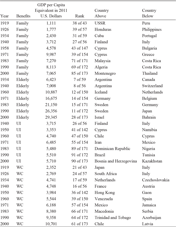
Table 7 shows the GDP per capita equivalent in 2011 U.S. dollars for the U.S. benefit in a specific year, its ranking relative to the number of countries with GDP per capita data, and the countries ranked immediately above and below the United States. The international rankings are not weighted by population. Information is available for fewer than 60 countries for the years prior to 1950. A large majority of the countries with no real GDP information prior to 1950 were probably ranked below the U.S. benefit levels. In later years, the median rank for those missing countries was between 91.5 and 114. Based on later rankings and the identities of the missing countries, the U.S. average elderly benefits ranking probably would have fallen no more than 2–5 spots, the WC benefits no more than 10 spots, and the family benefits no more than 10–15 spots if all of the countries were included prior to 1950.
INTERNATIONAL RANKING OF GDP PER CAPITA EQUIVALENTS OF BENEFIT LEVELS IN 2011 U.S. DOLLARS

Notes: The per capita benefits were determined by dividing the family benefits by the number of people in the family (either three or four depending on the year). Per capita benefits for WC benefits and unemployment insurance divided the benefit by four. The elderly benefit was for a one-person household. The benefits were converted to a GDP equivalent by multiplying the benefits by the ratio of (benefits + nontransfer government spending) to benefits. The government spending measure included education, police, national defense, administration, and courts and did not include government funds for public welfare, health and hospitals, employment security, veterans services, housing and community development, interest on general debt, liquor stores, and insurance trust funds.
Sources: The data on GDP in 2011 U.S. dollars comes from the Maddison Project Database version 2018.
The U.S. mean elderly target benefits always ranked very high, ranging from 7th to 15th through 1990 and then falling to 28th in 2000. They were roughly comparable to average per capita incomes in Japan and a number of European countries. The family target benefits ranked between 27th and 43rd through 1971, when they were comparable with per capita incomes in southeastern Europe, and then fell to the 69th–85th range, near some countries on the periphery of Europe and in Asia. Remember that the U.S. benefits would have received a substantial boost for those on public assistance who received the rent subsidies through HUD. WC maximum benefits per person in a four-person household ranked in the teens and twenties before 1950, similar to Japan, Italy, France, and Austria. They then fell back to rankings in the sixties out of around 170 countries, near Mexico, South America, and southern Europe, in 2000. UI maximums for a four-person household when annualized typically ranked in the 26th–55th range through 1971 and then fell to around the 90th range in later years. Keep in mind that the UI benefits are designed to last only for about six months in most cases.
CONCLUSION
Recasting the rise of the welfare state as the rise of the social insurance state has significant implications for public discourse in America. Social Security, Medicare, Disability Insurance, UI, and WC were all described to the public at their origins as programs with trust funds that were supposed to be used to fund future benefits. This meant that recipients and their employers perceived that they had contributed their appropriate share to the funds and no one could claim that recipients were the undeserving poor. Unemployment Insurance and WC have their glitches but tend to operate on basic insurance principles. Even though Roosevelt emphasized the insurance principles for Social Security, the pay-go structure of the program has led to significant disagreement about policies for dealing with the coming Social Security revenue shortfalls. Social insurance advocates argue that reducing the payroll contributions puts future benefits in jeopardy, eliminating the cap on income subject to taxation diminishes the relationship between contributions and benefits, and cutting benefits lowers the “return” on the individual’s contributions during their work life. Social Security was “saved” multiple times into the 1980s by quintupling the rates for payroll contributions and delaying the starting age of benefits. Since that time, immigration has helped the ratio of workers to beneficiaries, but there have been no more tax increases. Advocates of redistributive Social Security argue that the pay-go structure already has turned the program into transfers from workers to the elderly, which eliminates the restrictions on policy options described above. This raises the question about why Roosevelt and so many leaders since (think of Al Gore’s “lockbox”) have continued to emphasize the social insurance aspect in public claims. Apparently, a significant swath of the American voters still value the social insurance aspect of Social Security, Medicare, and Disability Insurance, possibly because social insurance does not carry the stigma of receiving welfare handouts.
The United States ranks fifth in public and private social welfare spending net of taxes relative to GDP among the OECD countries. The major difference between the United States and the European countries is in the mix of private and public spending. All of these countries are mixed economies that rely on markets and governments, and the majority of Americans have shown a preference for more reliance on markets than people in many of the other countries. The differences were more extreme in the 1980s than they were by the year 2000, as many of the European countries have loosened their regulations to allow households to buy private health insurance to supplement the health services offered by governments and many have backed away from wealth taxes and high tax rates on high earners.
Social welfare expenditures and the number of recipients tell only part of the story for public assistance and social insurance policies, because the public assistance programs still focus on budget-deficit principles in which they seek to fill the gap between a household’s resources and a target budget. Spending per recipient can only provide inferences about the level of these targets because it is so heavily influenced by the difference between the target and recipient incomes.
Public assistance programs have been more generous to the elderly poor than to families. National average real benefits have risen substantially over the course of the century. The benefits rose faster than the poverty line, as well as state manufacturing earnings and benefits, and kept pace with per capita incomes in the states. Elderly poor recipients also fared well in comparisons of a GDP equivalent of their benefits with average incomes in foreign countries, ranking in the top 30 in all years compared. Since the introduction of Medicaid, much of the benefit rise has come from increased medical expenditures, which grew faster for the elderly poor than for Medicare recipients and much faster than for poor families.
Through 1990, family benefit targets also rose in real terms and rose relative to the poverty line and manufacturing earnings and benefits, while maintaining a ratio to state per capita income in a range of 0.21–0.25. The TANF reforms, however, contributed to a drop in real benefits, as nonmedical benefits fell. Before 1971, family target benefits were comparable to per capita incomes for countries ranked between 27th and 43rd, but their ranking fell to the 69th–85th range out of 170 countries afterward.
The real national average weekly maximums for both UI and WC fell sharply between 1940 and 1950, as state legislatures failed to update the maximums in response to the rise in wages and incomes. Afterward, real WC maximums rose for the rest of the century, outpacing the four-person poverty line and state manufacturing earnings and benefits and keeping pace with state per capita incomes. Unemployment Insurance average maximums also rose through 1971 but ended up below that 1971 maximum for the rest of the century and, thus, did not keep pace with the three income standards. The differences in trends between the two programs likely came about because far more states indexed their benefits to state average wages under WC than under UI. The indexing overcame a standard problem for social welfare programs that arises when benefit changes have to be legislated from year to year.
My goal has been to provide an overview of the trends in social insurance and public assistance programs in the twentieth century. The paper only shows long-term trends based on information from one year in each decade. The United States has 51 or more versions of these programs, and I have only shown a small amount of that variation in the paper. More information is available in the dataset posted online to accompany the paper. Understanding the forces that determined the changes in the targets and their impact requires filling in more years in the panel dataset for each of the states for each program. One key issue that I only began to address was the importance of cross-sectional differences in the cost of living. When states have chosen a wide range of nominal targets, adjustments for cost of living tend to reduce the variance of the distribution of targets, can shift the purchasing power substantially for a number of states, and can substantially change correlations between benefits. In situations where states tend to choose a narrow range of benefits, cost-of-living adjustments spread the distribution of benefits and low-cost states, often southern, lead the rankings. More work needs to be done to collect and improve upon existing cross-sectional measures and build new measures of cross-sectional purchasing power.
In international comparisons of the United States and other countries related to social welfare issues (and also many other economic issues), more attention needs to be paid to the diversity of benefit targets across states. This might be true in other countries, such as China, that span large areas. The international comparisons between the U.S. national average and countries in Table 7 show that the U.S. target benefits are higher than average incomes in quite a few countries. But that is really only the starting point for comparison because U.S. benefits likely vary as much or more as incomes and benefits across Europe. Table 6 shows that the target benefit in Alaska would rank high relative to average foreign incomes, while the target in Alabama would rank relatively low.