2. Acoustic coupled mode theory

Let us start with the formulation of the problem. Throughout this paper we adopt non-dimensionalized quantities. After the time dependence is removed through the substitution ${\it\psi}(t)={\it\psi}\exp (-\text{i}{\it\omega}t)$ , the pressure field ${\it\psi}$ within a cavity–duct structure is controlled by the non-dimensional stationary Helmholtz equation

where ${\it\omega}$ is the non-dimensional frequency. The $x$ -axis is aligned with the centreline of the duct–cavity structure. The problem could be reduced to two dimensions under assumption that the structure has constant thickness along the $z$ -axis which allows us to present the solution of (2.1) as ${\it\psi}={\it\psi}(x,y){\it\psi}(z)$ . In what follows we take ${\it\psi}(z)=\text{const}.$ which means that only the first propagating mode is involved.

Equation (2.1) has to be solved subject to Neumann boundary conditions on all sound-hard boundaries of the cavity and reflectionless boundary conditions on the cavity–waveguide interfaces. There are numerous numerical techniques for imposing reflectionless conditions on waveguide–cavity interfaces, the most efficient of which implement layers of absorbing medium with complex refractivity giving rise to perfectly matched layers (Berenger Reference Berenger1994) or complex scaling (Moiseyev Reference Moiseyev1998) methods. For detailed information on the use of these methods for finding acoustic BSCs we refer the reader to the papers by Hein & Koch (Reference Hein and Koch2008), Hein et al. (Reference Hein, Koch and Nannen2012) which thoroughly review the subject. In this paper we will use an alternative method, namely acoustic coupled mode theory (Maksimov et al. Reference Maksimov, Sadreev, Lyapina and Pilipchuk2015). The method is a recent adaptation of the approach known in quantum mechanics as formalism of the effective non-Hermitian Hamiltonian. In this section we only briefly review the essentials and introduce the basic concepts that will be needed later on for understanding the mechanism of BSC formation.

Figure 1.

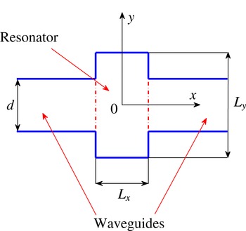
Structure lay-out. $d=1$ .

To be consistent with the further applications our approach is exemplified on the two-dimensional duct–cavity structure depicted in figure 1 where we show a two-dimensional cavity of length $L_{x}$ and width $L_{y}$ coupled to symmetrically positioned waveguides of width  $d$ . In what follows we take $d=1$ . As mentioned in the Introduction the coupled mode theory relies on the spectral properties of a closed cavity decoupled from the waveguides. In that context closed means that in the first step the eigenmodes and eigenfrequencies of the cavity are computed with the Neumann boundary conditions

on the boundary of the resonator $\partial {\it\bf\Omega}$ , including the waveguide–cavity interfaces as well as the physical boundaries; ${\it\sigma}$ is the local coordinate normal the boundary of the closed resonator. In the case of a rectangular cavity the eigenvalue problem is easily solved analytically to yield the spectrum as

At the same time the eigenmodes are found as products of two factors:

where ${\it\delta}_{n^{\prime }}^{n}$ is the Kronecker delta. Note that the eigenfunctions are unit-normalized, so that

The propagating solutions in the waveguides have the form of plane waves:

where symbol $+(-)$ stands for waves propagating to the right (left), and the functions ${\it\chi}_{p}(y)$ are defined as

The dispersion relation is

The pressure field within the cavity ${\it\psi}_{c}$ could be constructed as a modal expansion

over eigenfunctions (2.4). The key equation for finding the unknowns $g_{n,m}$ for the cavity excited by an incoming wave has the following form (Maksimov et al. Reference Maksimov, Sadreev, Lyapina and Pilipchuk2015):

where $\unicode[STIX]{x1D644}$ is the identity matrix, the subscript $C=L,R$ specifies the coupling with the left and right waveguides, and the unknown vector $\boldsymbol{g}$ contains the coefficients $g_{n,m}$ . Analogously, the amplitudes $a_{C,p}$ are the coefficients of the modal expansion of the incident wave field in the waveguides over the eigenfunctions (2.6), while the vector $\boldsymbol{v}_{C,p}$ contains the coupling constants $v_{C,p}^{m,n}$ between the specific eigenmode $(m,n)$ (2.4) and the $(C,p)$ propagating mode of the waveguides (2.6). Finally, the matrix $\unicode[STIX]{x1D63F}$ has the following form:

where ${\it\bf\Omega}^{2}$ is a diagonal matrix which carries the squared eigenfrequencies ${\it\omega}_{n,m}^{2}$ (2.3) on the main diagonal and the symbol $\dagger$ stands for Hermitian transpose. Notice that the coupling to the evanescent modes $(p-1){\rm\pi}>{\it\omega}$ of the waveguides is accounted for in (2.11) by the terms with imaginary wavenumbers $k_{p}$ found from (2.8). At this point we only have to specify the coupling constants $v_{C,p}^{n,m}$ . According to Pichugin et al. (Reference Pichugin, Schanz and Seba2001) and Maksimov et al. (Reference Maksimov, Sadreev, Lyapina and Pilipchuk2015) they are evaluated as overlapping integrals between the functions (2.7) and the eigenfunctions (2.4) on the waveguide–cavity interface:

where ${\it\tau}_{C}$ is the local interface coordinate orthogonal to the wave vector. The generalization to the three-dimensional case is straightforward; the coupling constant is a surface integral (Maksimov et al. Reference Maksimov, Sadreev, Lyapina and Pilipchuk2015) with ${\it\tau}_{C}$ representing the local coordinate set on a flat waveguide-resonator interface. Notice that (2.10) formally contains an infinite number of unknowns. However, as it was demonstrated in Maksimov et al. (Reference Maksimov, Sadreev, Lyapina and Pilipchuk2015), for computational ease the basis can be truncated to a reasonably small number of modes in a given frequency window. After the unknown vector $\boldsymbol{g}$ is obtained from (2.10) the coefficients of the modal expansion of the outgoing field in the waveguide $b_{C,p}$ are found as

The above described approach has been demonstrated to be applicable to finding scattering functions and reflection amplitudes in two- and three-dimensional cavities (Maksimov et al. Reference Maksimov, Sadreev, Lyapina and Pilipchuk2015). The goal of the present paper, however, is to adapt it for computing BSCs. The BSCs are localized solutions of infinite life-time which exist in the cavity even when no incident field is present in the waveguides. Thus, according to (2.10) one obtains an eigenvalue problem

When an eigenvalue $z_{n}={\it\omega}_{n}+\text{i}{\it\gamma}_{n}$ found from (2.14) is real its eigenvector $g_{n}$ corresponds to a BSC. Unfortunately, (2.14) does not represent the standard eigenvalue problem because the matrix $\unicode[STIX]{x1D63F}$ (2.11) depends on the spectral parameters $k_{p}$ which are linked to the eigenvalue $z_{n}$ through the dispersion relation (2.8). One of the possible solutions (Sadreev et al. Reference Sadreev, Bulgakov and Rotter2006) is to employ an iterative procedure of solving the fixed-point equation for real eigenvalues of (2.14). Alternatively, one of the most efficient techniques for finding complex eigenvalues (2.14) is the harmonic inversion method which allows one to extract the positions and life-times of the resonances from the response of the system to an external driving. In this paper we do not detail the harmonic inversion method as Wiersig & Main (Reference Wiersig and Main2008) nicely outline it in their paper on the fractal Weyl law for chaotic microcavities. In brief, the first step in the method is solving (2.10) with some, quite arbitrary, right-hand side which, in particular, could be a point source placed within the open cavity. The response obtained is then Fourier-transformed to yield a set of nonlinear equation for eigenvalues $z_{n}$ which is subsequently solved by the use of Padé approximants (Wiersig & Main Reference Wiersig and Main2008).

To conclude this section we return to the Friedrich–Wintgen two-mode interference mechanism of BSC formation (Friedrich & Wintgen Reference Friedrich and Wintgen1985). Let us check whether it is possible that only two modes ${\it\psi}_{1}$ and ${\it\psi}_{2}$ of the closed cavity with eigenfrequencies ${\it\omega}_{1}$ and ${\it\omega}_{2}$ contribute to a BSC. Suppose that only the first scattering channel with the wavenumber $k_{1}$ is open at the frequency of interest. Then, under a further assumption that the coupling to the evanescent channels $p>1$ can be neglected we rewrite (2.14) as an eigenvalue problem for matrix $\unicode[STIX]{x1D63F}$ with real-valued terms ${\it\omega}_{j}^{2}$ arranged along the main diagonal in ascending order:

where ${\it\omega}_{0}$ and ${\it\omega}_{3}$ are the eigenfrequencies next to ${\it\omega}_{1}$ and ${\it\omega}_{2}$ , and $v_{j}=v_{L,1}^{m,n}$ is the coupling constant with the open propagation channel $p=1$ . Notice that above we have assumed that the absolute values of the coupling constants on the left and the right are identical, i.e. all eigenmodes have compatible symmetry about the $y$ -axis. In fact, the matrix $\unicode[STIX]{x1D63F}$ is split into two decoupled sub-blocks corresponding to the $y$ -symmetric and $y$ -antisymmetric eigenmodes so that the $y$ -symmetric and $y$ -antisymmetric problems could be considered independently from one another. Under variation of some control parameter, say the length of the cavity $L_{x}$ , one can reach the degeneracy point where ${\it\omega}_{1}={\it\omega}_{2}={\it\omega}_{BSC}$ ; then the matrix (2.15) has a real eigenvalue ${\it\omega}_{BSC}^{2}$ with the eigenvector

containing only two non-zero entries. Thus, the corresponding BSC shape function can be constructed as

The above equation represents the central mathematical result to be used for analyzing BSCs in open acoustic resonators. In essence, it manifests the well-known interference mechanism (Friedrich & Wintgen Reference Friedrich and Wintgen1985). In fact, both eigenmodes ${\it\psi}_{1}$ and ${\it\psi}_{2}$ , albeit coupled to the waveguides, contribute to (2.17) in the proportion providing full destructive interference at the degeneracy point so that the resulting BSC function ${\it\psi}_{BSC}$ is decoupled from the open channel. For details on the realization of the above mechanism in the field of quantum mechanics we refer the reader to the paper by Sadreev et al. (Reference Sadreev, Bulgakov and Rotter2006). We mention in passing that thanks to the symmetry about the duct axis the same arguments are valid for the duct-axis antisymmetric modes with $k_{1}$ replaced by $k_{2}$ according to (2.8).

Table 1.

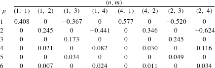
Numerical values of coupling constants $v_{L,p}^{n,m}$ at $L_{x}=3,L_{y}=2$ .

The above result (2.17) is exact under the assumption that the coupling to the evanescent channels could be neglected. However, we would like to remind the reader that the evanescent eigenmodes are present in summation over index $p$ on the right-hand side of (2.11). Therefore (2.17) is not an exact solution, and can only be seen as the basis for a two-mode approximation for BSCs occurring at the degeneracy points. Some remarks are due on the validity of the two-mode approximation. As will be seen later on, due to the structure of (2.11) the evanescent coupling results in the presence of modes other than the two basic modes in the modal expansion of the BSC shape function, as well as in a shift of the true BSC point from the degeneracy point. Nevertheless, one can argue that the coupling to the evanescent channels is small relative to the coupling to the open channel as we consider the eigenmodes residing in the frequency window where only one symmetric and one antisymmetric propagating channel are open. In order to illustrate this we collect in table 1 the numerical values of the coupling constants for some relevant eigenmodes evaluated on the basis of the analytical results from Maksimov et al. (Reference Maksimov, Sadreev, Lyapina and Pilipchuk2015). One can see from table 1 that the coupling constants rapidly decay with the growth of the channel number  $p$ . In fact, in can be demonstrated that any coupling constant decays away from its maximal value with the asymptotic law $v_{L,p}^{n,m}\sim 1/p^{2}$ .

Finally, notice that the two-mode approximation has no restrictions related to the size of the cavity. One can see from (2.15) that once a degeneracy occurs in the closed cavity it always results in the formation of a BSC through the Friedrich–Wintgen mechanism irrespective of the values of $L_{x}$ , and $L_{y}$ . If the size of the cavity is isometrically increased while the width of the waveguide is kept unchanged, the eigenfrequencies next to the BSC eigenfrequencies ${\it\omega}_{0},{\it\omega}_{3}$ would shift closer to the BSC eigenfrequency. The real-valued diagonal term in (2.14) will decrease as $({\it\omega}_{0,3}^{2}-{\it\omega}_{BSC}^{2})\sim 1/S,S=L_{x}L_{y}$ because the mean distance between the eigenfrequencies is inversely proportional to the width/length of the cavity. On the other hand the coupling constants $v_{j}$ in matrix $\unicode[STIX]{x1D63F}$ (2.15) will decrease as $v_{j}\sim 1/\sqrt{S}$ because the eigenfunctions (2.4) contributing to the overlapping integrals (2.12) have the normalization constant $\sqrt{S}$ in the denominator. As a consequence of this the off-diagonal terms $v_{j}v_{j^{\prime }}$ in matrix (2.15) decrease as $v_{j}v_{j^{\prime }}\sim 1/S$ . One can see that the coupling of the BSC eigenmodes ${\it\psi}_{0}$ , ${\it\psi}_{3}$ next to the basic BSC modes ${\it\psi}_{1}$ , ${\it\psi}_{2}$ through the evanescent channels decreases at the same rate as the resonant term ${\it\omega}_{0,3}^{2}-{\it\omega}_{BSC}^{2}$ . This leads us to the conclusion that the two-mode approximation does not break down as the size of the cavity is increased. Notice that the same holds true in the three-dimensional case where the coupling constant decreases as $v_{j}\sim 1/\sqrt{V}$ , with $V$ being the volume of the cavity.

3. Bound states in the continuum in two-dimensional open cavities

We start by computing the transmittance $T=|b_{1,R}|^{2}$ for the two-dimensional cavity in figure 1 under the assumption that an incident wave in the first propagation band $p=1$ enters the cavity from the left waveguide. For solving the scattering problem we used the approach described in § 2. The numerical values of the coupling constants $v_{C,p}^{n,m}$ in (2.10), (2.11) are taken from our previous work (Maksimov et al. 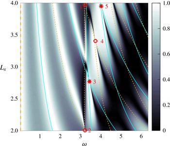Reference Maksimov, Sadreev, Lyapina and Pilipchuk2015). In figure 2 we demonstrate the dependence of the transmittance $T$ on the frequency of the incoming wave ${\it\omega}$ and the length of the cavity $L_{x}$ . Notice that the frequency varies in the range $[0,2{\rm\pi}]$ which means according to (2.8) that only one symmetric scattering channel is open in each waveguide. In figure 2 we also depict the frequencies of the eigenmodes of the closed cavity symmetric about the duct axis (2.3) $m=1,3,5,\ldots .$ The eigenfrequencies which correspond to the modes symmetric about the $y$ -axis, to be referred to below as $y$ -symmetric, are shown by dashed lines. The solid lines show the eigenfrequencies of $y$ -antisymmetric eigenmodes. One can see that the degeneracy points of eigenfrequencies with the same symmetry about the $y$ -axis coincide with an abrupt change of the transmittance; the transmittance drops from unity to zero as the frequency is swept across the point where the collapse of Fano resonance occurs.

Figure 2.

Transmittance for a two-dimensional cavity of length $L_{y}=2$ . Only the first symmetric channel with $p=1$ is open. The dashed lines show eigenfrequencies of the modes symmetric about the $y$ -axis; the solid lines show antisymmetric ones. The positions of the BSCs are shown by open circles and stars for $y$ -symmetric and $y$ -antisymmetric modes, respectively.

Figure 3.

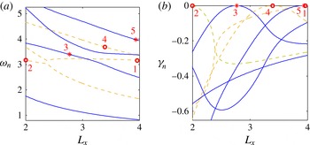
Complex eigenfrequencies against the length of the two-dimensional resonator $L_{x}$ : (a) real part; (b) imaginary part. The $y$ -symmetric resonances are shown by dashed lines; the $y$ -antisymmetric ones by solid lines. The positions of BSCs from figure 2 are shown by open circles and stars for $y$ -symmetric and $y$ -antisymmetric modes, respectively.

Figure 4.

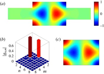
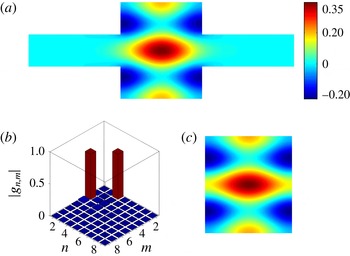
BSC 3, symmetric about the duct axis of a two-dimensional duct–cavity structure with ${\it\omega}_{BSC}=3.396,L_{y}=2,L_{x}=2.776$ : (a) pressure field of the numerically computed BSC shape function; (b) absolute values of the modal coefficients $g_{n,m}$ of the numerically computed pressure field (2.9); (c) BSC shape function found from the two-mode approximation (2.17).

The complex resonance frequencies for the cavity are computed by the harmonic inversion method. In the given range of parameters we found five BSCs. Three of them originate from the modes symmetric about the $y$ -axis (shown by circles) and two from the antisymmetric ones (shown by stars). For further convenience we number the BSCs from 1 to 5. The complex eigenfrequencies are plotted against the length of the resonator $L_{x}$ in figure 3 where one can see that the imaginary part ${\it\gamma}_{n}$ goes to zero as one approaches the BSC point. In figure 4 we demonstrate the numerical solution for BSC 3 along with the corresponding coefficients of the modal expansion $g_{n,m}$ (2.9). One can clearly see that only two eigenmodes dominate in the BSC function ${\it\psi}_{BSC}$ . The $y$ -antisymmetric BSC 3 in figure 4 is formed by eigenmodes ${\it\psi}_{1}={\it\psi}_{4,1}(x,y)$ and ${\it\psi}_{2}={\it\psi}_{2,3}(x,y)$ , with the corresponding coupling constants $v_{1}=v_{L,1}^{4,1}=-v_{R,1}^{4,1}=0.600$ and $v_{2}=v_{L,1}^{2,3}=-v_{R,1}^{2,3}=-0.540$ . To assess the accuracy of the two-mode approximation we introduce parameters

and

with ${\it\omega}^{\ast }$ and $L_{x}^{\ast }$ respectively the frequency and the length of the cavity corresponding to the degeneracy point at which the BSC would occur according the two-mode approximation (2.15). For BSC 3 we obtained ${\rm\Delta}{\it\omega}=0.019$ and ${\rm\Delta}L_{x}=0.018$ . In figure 4 we also plot the BSC shape function constructed by (2.17). One can see from figure 4 that the two-mode approximation reproduces our numerical result to a good accuracy. We found that the same holds true for the other four BSCs in figure 2. Therefore, the other BSC functions are not presented in this paper.

Figure 5.

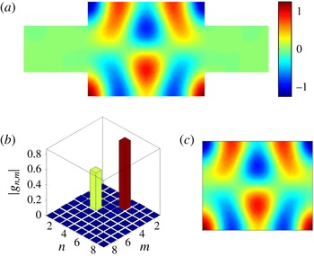
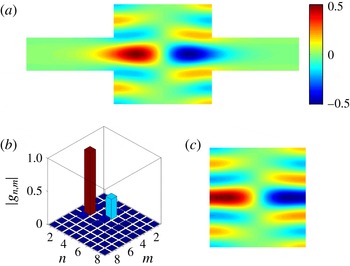
Bound state in the continuum antisymmetric about the duct axis of a two-dimensional duct–cavity structure with ${\it\omega}_{BSC}=5.385,L_{y}=2,L_{x}=2.441$ : (a) pressure field of the numerically computed BSC shape function; (b) absolute values of the modal coefficients $g_{n,m}$ of the numerically computed pressure field; (c) BSC shape function found from the two-mode approximation (2.17).

Figure 6.

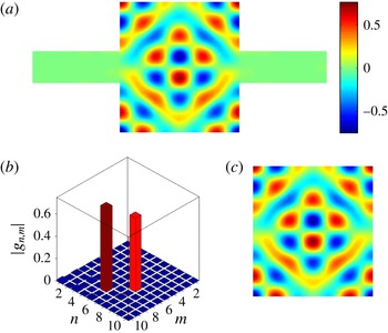
Bound state in the continuum antisymmetric about the duct axis of a two-dimensional duct–cavity structure with ${\it\omega}_{BSC}=6.502,L_{y}=4,L_{x}=3.627$ : (a) pressure field of the numerically computed BSC shape function; (b) absolute values of the modal coefficients $g_{n,m}$ of the numerically computed pressure field; (c) BSC shape function found from the two-mode approximation (2.17).

The same procedure was repeated in the case of the incoming wave in the first antisymmetric channel for cavities with $L_{y}=2$ . As before we observed that the two-mode approximation is valid in the situation when only one antisymmetric channel is open in each waveguide. For brevity we omit a detailed description of our findings, restricting ourselves to one example of a duct-axis antisymmetric BSC, shown in figure 5. The $y$ -symmetric BSC in figure 5 is formed by eigenmodes ${\it\psi}_{1}={\it\psi}_{5,2}(x,y)$ and ${\it\psi}_{2}={\it\psi}_{3,4}(x,y)$ , with the corresponding coupling constants $v_{1}=v_{L,1}^{5,2}=v_{R,1}^{5,2}=-0.692$ and $v_{2}=v_{L,1}^{3,4}=v_{R,1}^{3,4}=0.384$ . For the corresponding relative errors (3.1), (3.2) we found ${\rm\Delta}{\it\omega}=0.004$ and ${\rm\Delta}L_{x}=0.004$ . As mentioned in § 2, we expect that the two-mode approximation could be applied irrespective of the cavity size. This is confirmed by numerical tests for larger cavities $L_{y}=4$ . As an example, in figure 6 we present the duct-axis antisymmetric BSC formed by eigenmodes ${\it\psi}_{1}={\it\psi}_{5,8}(x,y)$ and ${\it\psi}_{2}={\it\psi}_{7,6}(x,y)$ , with the coupling constants $v_{1}=v_{L,1}^{5,8}=v_{R,1}^{5,8}=-0.371$ and $v_{2}=v_{L,1}^{7,6}=v_{R,1}^{7,6}=0.402$ . The values of the relative errors ${\rm\Delta}{\it\omega}=0.003$ and ${\rm\Delta}L_{x}=0.007$ indicate that the two-mode approximation holds true for larger cavities.

Figure 7.

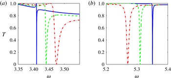
Collapse of Fano resonance in the vicinity of a BSC point under variation of the length of the resonator $L_{x}$ . (a) BSC 4 in figure 4 with ${\it\omega}_{BSC}=3.396,L_{y}=2,L_{x}=2.776$ . Resonator lengths: $L_{x}=2.75$ , solid line; $L_{x}=2.70$ , dashed line; $L_{x}=2.60$ , dash-dot line. (b) Duct-axis antisymmetric BSC in figure 5 with ${\it\omega}_{BSC}=3.384,L_{y}=2,L_{x}=2.441$ . Resonator lengths: $L_{x}=2.460$ , solid line; $L_{x}=2.485$ , dashed line; $L_{x}=2.510$ , dash-dot line.

Figure 8.

Scattering function at the peak ${\it\omega}=3.410$ of the Fano resonance in figure 7 related to BSC 3 shown in figure 4. $L_{y}=2,L_{x}=2.75$ . (a) Real part; (b) imaginary part.

As mentioned in the Introduction, the occurrence of a BSC is associated with a collapse of Fano resonance. To illustrate this, in figure 7 we plot the transmittance versus frequency for three different lengths of the resonator $L_{x}$ close to the BSC points. It was recently demonstrated by Bulgakov & Sadreev (Reference Bulgakov and Sadreev2014) that if the BSC point is approached in the parametric space along a certain path corresponding to the peak of the Fano resonance, the long-lived complex mode related to the BSC provides the dominant contribution to the scattering function. In consequence the scattering function near the BSC point bears the maximal resemblance to the BSC if the parameters are tuned to the peak of the Fano resonance. This is illustrated in figure 8, where one can see that the real part of the scattering function is almost identical to the BSC from figure 4, whereas the imaginary part is present as a background providing the net power flux in the system. Thus, one can experimentally observe a signature of a BSC in the form of a large-amplitude acoustic resonance even though in a realistic set-up the parameters are always detuned from the true BSC point due, for example, to fabrication inaccuracies.

Figure 9.

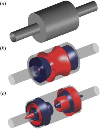
Bound states in the axisymmetric duct–cavity structure. (a) Cylindrical resonator of radius $R$ and length $L_{x}$ with two coaxially attached waveguides of radius $a=1$ . (b) Pressure field isosurfaces of BSC 2 in figure 12 symmetric with respect to the central section of the resonator; dark blue ${\it\psi}_{BSC}=-0.1$ , light red ${\it\psi}_{BSC}=0.1$ . (c) Pressure field isosurfaces of BSC 7 in figure 13 antisymmetric with respect to the central section of the resonator; dark blue ${\it\psi}_{BSC}=-0.1$ , light red ${\it\psi}_{BSC}=0.1$ .

Figure 10.

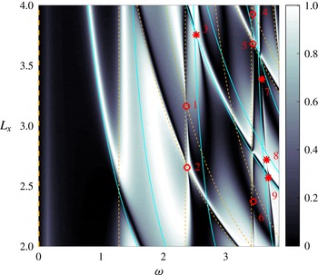
Transmittance for a cylindrical resonator with radius $R=2$ with two coaxially attached cylindrical waveguides of radius $a=1$ versus frequency ${\it\omega}$ and the length of the resonator $L_{x}$ . The dashed lines show eigenfrequencies of the modes symmetric about the $y0z$ -plane; solid lines show antisymmetric ones. The positions of the BSCs are shown by open circles and stars for $y0z$ -symmetric and $y0z$ -antisymmetric modes, respectively.

Figure 11.

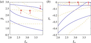
Complex eigenfrequencies against the length of the three-dimensional resonator $L_{x}$ : (a) real part, (b) imaginary part. The $y0z$ -symmetric resonances are shown by dashed lines; $y0z$ -antisymmetric ones by solid lines. The positions of BSCs from figure 10 are shown by open circles and stars for $y0z$ -symmetric and $y0z$ -antisymmetric modes, respectively.

Figure 12.

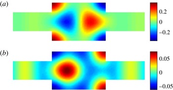
BSC 2 in a three-dimensional duct–cavity structure with ${\it\omega}_{BSC}=2.367,R=2,L_{x}=2.655$ : (a)  $x0y$ -plane section of the pressure field of the numerically computed BSC shape function; (b) absolute values of the modal coefficients of the numerically computed pressure field; (c) BSC shape function found from the two-mode approximation (2.17).

Figure 13.

BSC 7 in a three-dimensional duct–cavity structure with ${\it\omega}_{BSC}=3.557,R=2,L_{x}=3.387$ : (a)  $x0y$ -plane section of the pressure field of the numerically computed BSC shape function; (b) absolute values of the modal coefficients of the numerically computed pressure field; (c) BSC shape function found from the two-mode approximation (2.17).

4. Bound states in the continuum in three-dimensional open cavities

Let us consider the axisymmetric cylindrical resonator with two coaxially attached cylindrical waveguides of radius $a=1$ as depicted in figure 9(a). After the azimuthal variable is separated out we can restrict ourself to the case of zero angular momentum, bearing in mind that our results can be easily generalized to the non-zero case by taking into account that, by virtue of (2.12), only the modes of the same rotational number are coupled on the waveguide–cavity interface. In our case the cavity eigenfrequencies are given by

where $R$ and $L_{x}$ are the radius and length of the cylindrical resonator, and ${\it\mu}_{m}$ is the $m$ th root of the equation $\text{J}_{0}^{\prime }({\it\mu}_{m})=\text{J}_{1}({\it\mu}_{m})=0,m=1,2,\ldots \,$ , for the derivative of the first-order Bessel function. The corresponding eigenfunctions are

where $r$ is the radial coordinate in the $y0z$ -plane while the axial modes are given by

As before the transmission problem was solved by the use of the acoustic coupled mode theory (Maksimov et al. Reference Maksimov, Sadreev, Lyapina and Pilipchuk2015) and the complex eigenvalues were obtained by the harmonic inversion method. The frequency ${\it\omega}$ varies in the range $[0,{\it\mu}_{2}],{\it\mu}_{2}=3.831$ which means that only one propagating channel is open in each waveguide. The transmittance, along with the spectrum of the closed resonator and the positions of BSCs, is shown in figure 10. The complex eigenfrequencies are plotted in figure 11 against the length of the resonator $L_{x}$ . In figures 12 and 13 we demonstrate the shape functions of two BSCs occurring through the two-mode interference mechanism. BSC 2 in figure 12 with ${\rm\Delta}{\it\omega}=0.012$ and ${\rm\Delta}L_{x}=0.012$ is formed by eigenmodes ${\it\psi}_{1}={\it\psi}_{1,3}(r,x)$ and ${\it\psi}_{2}={\it\psi}_{3,1}(r,x)$ , with the corresponding coupling constants $v_{1}=v_{L,1}^{3,1}=v_{R,1}^{3,1}=0.310$ and $v_{2}=v_{L,1}^{1,3}=v_{R,1}^{1,3}=0.289$ , while the $y0z$ -antisymmetric BSC 7 depicted in figure 13 is formed by ${\it\psi}_{1}={\it\psi}_{2,4}(r,x)$ and ${\it\psi}_{2}={\it\psi}_{4,3}(r,x)$ , with the coupling constants $v_{1}=v_{L,1}^{2,4}=-v_{R,1}^{2,4}=-0.078$ and $v_{2}=v_{L,1}^{4,3}=-v_{R,1}^{4,3}=0.389$ . A three-dimensional visualization of BSCs from figures 12 and 13 is offered in figure 9(b,c) in the form of pressure field isosurfaces. One can see that, of all the BSCs in figure 10, BSC 7 deviates the most from the corresponding degeneracy point ${\rm\Delta}{\it\omega}=0.016$ and ${\rm\Delta}L_{x}=0.066$ . The reason for this can be understood from figures 9(c) and 13 where one can clearly see that BSC 7 extends far into the waveguides due to the coupling to the evanescent modes which is neglected by the two-mode approximation. One can conclude that the coupling to the evanescent modes becomes important just below the next channel propagation threshold as the channel function extends far into the waveguide. Nevertheless, the two-mode approximation is still valid in the three-dimensional case, reproducing the numerically computed shape functions to a good accuracy.

In this paper, we restricted ourself to coaxial systems in which the azimuthal number is a constant of motion so that the rotational vibration modes do not participate in the formation of BSC depicted in figures 12 and 13. It is worth noticing, however, that the cavity eigenmodes with azimuthal number ${\it\nu}\neq 0$ are symmetry-protected BSCs as their eigenfrequencies are below the ${\it\nu}$ th propagating threshold in cylindrical waveguides.