1 Introduction
Computers have increasingly taken over tedious and repetitive tasks from human researchers. From counting words in a file to performing long and complex calculations, machines are able to follow a set of instructions in a repetitive manner without fatigue or cognitive bias. Their capacity to perform quickly and reliably allows social scientists to analyze information from a large amount of data, such as roll-call votes (McCarty, Poole, and Rosenthal Reference McCarty, Poole and Rosenthal2006), congressional floor speeches (Dietrich, Enos, and Sen Reference Dietrich, Enos and Sen2019; Dietrich, Hayes, and O’Brien Reference Dietrich, Hayes and O’Brien2019), and social media posts (Barberá Reference Barberá2015).
And yet, computers’ ability to follow a set of instructions used to be their chief limitation when dealing with visual information. In principle, for a computer to search for images where a specific political leader appears, we could create a checklist describing the physical characteristics of the individual (e.g., the form of her nose, the distance of her nose to her eyes, and the size of her forehead). But the directives could turn out to be insufficient when working with pictures in which the individual is not facing the camera, wears sunglasses, or appears in pictures with different lightings. Of course, we could help the computer by providing more rules, but the instruction list would be as vast as the number of ways in which an individual may appear in a picture.
Recent developments in computer science retrieve information from images using an alternative approach. Inspired by the way in which humans identify visual patterns, computers are exposed to multiple examples that allow them to extract and associate visual features with labels by transforming images into vectors of pixel values. These vectors capture colors, edges, textures, and other important features of the image, enabling computers to glean general patterns without following a specific set of rules. This approach has made it possible to classify visual content, recognize specific objects, or gather recognized objects into clusters.
To describe this technique, this paper introduces the use of convolutional neural networks (CNNs) as a reliable, cost-effective tool to deal with visual information. In particular, we present this method as an alternative way for analyzing, coding, and classifying large-scale image collections. We illustrate the advantages of this methodology by applying a CNN model to code handwritten information from vote tallies. This example allows us to explain the structure and functioning of CNNs in an intuitive and reliable way. Our main goal is to provide general guidelines for researchers who might want to use CNNs for their own projects.Footnote 1
At the same time, we also want to stress the limitations of this method. Valid concerns regarding CNNs stem from their opacity when linking the inputs and the model outputs (Zeiler and Fergus Reference Zeiler and Fergus2014; Nguyen, Yosinski, and Clune Reference Nguyen, Yosinski and Clune2015; Sabour, Frosst, and Hinton Reference Sabour, Frosst and Hinton2017), and their reliance on large and high quality training data. These warnings should deter scholars from applying this method to identify latent dimensions or ambiguous features in the data. We emphasize the importance of establishing transparent goals when using the model, avoiding post hoc interpretations of the outcomes, and restricting the use of CNNs to tasks that could be performed, in principle, by a human (Lipton Reference Lipton2016).
The manuscript is organized as follows. First, we introduce what CNNs are and the stages that these involve. Second, we list the process of building a CNN as well as a few technical and practical recommendations when applying these tools. Third, we also discuss the limitations of CNNs for certain measurement and classification tasks. Fourth, we illustrate the practicability of this tool using an electoral example involving the recognition of handwritten digits. We conclude by suggesting potential ways to expand the use of visual analysis in social sciences, as well as other avenues of research designed to improve and complement the use of CNNs for image classification.
Finally, we acknowledge that the method includes plenty of jargon. While we try to explain many of these concepts in terms most familiar to political scientists, a glossary at the end of the manuscript provides technical details about each of these terms, which we identify with italics in the main text.
2 A Primer on CNNs
A CNN is a model that takes an input (in the context of this article, images) and that assigns importance or “weights” to various features of such inputs in order to differentiate one from the other. The CNN has a structure of elements and specifications called the architecture, which has the concept of “convolution” at its core.
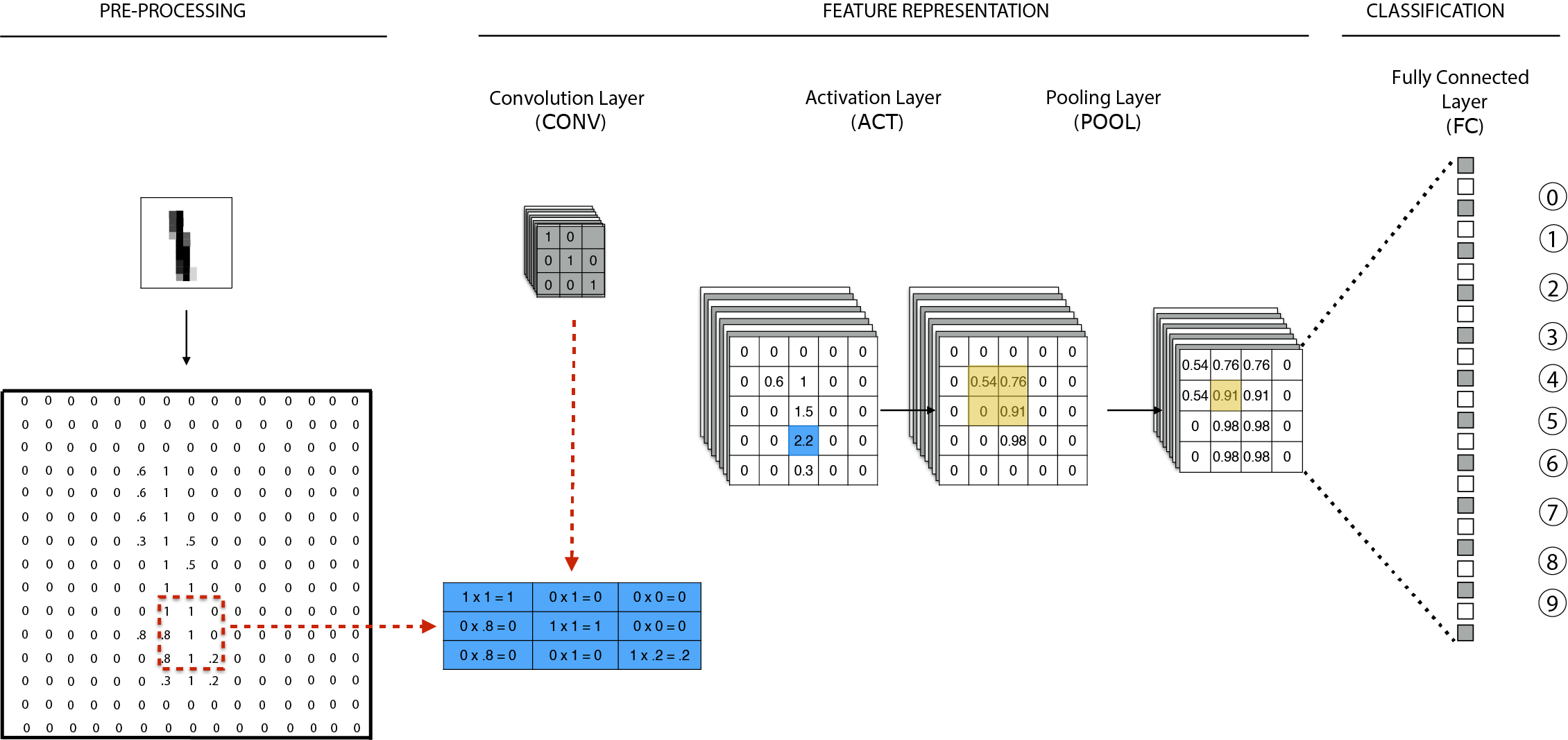
Figure 1 illustrates the basic architecture of a CNN, which is represented as a stack of different layers. Convolution layers (CONV) look for specific patterns in the feature space of the image. Activation (ACT) and pooling (POOL) layers perform numeric operations to introduce nonlinearities and reduce the dimensionality of the space respectively. Finally, the fully connected (FC) layer learns the parameters that help the model to classify the image in an accurate way. Altogether, this structure reduces the dimensionality of images and learns their content by looking for informative features and patterns across examples. We detail all of these concepts below.
The functionality of CNNs can be divided into three stages. The first one preprocesses the images to make sure they all share the same pixel area and range. The second stage deconstructs the images into multiple components, each representing a specific visual feature, and reduces the dimensionality of the data. The last stage gleans relevant information to classify the images into the available output labels. We explain below the logic behind each of these stages, the hyperparameters that each of them involves, and the alternatives available to the researcher. For ease of explanation, the illustrating example is based on images of handwritten numbers with a single color channel (i.e., the images are in grayscale). However, all the steps and details are easily extendable to colored images and their respective three color channels.
Example of a convolutional neural network structure.

2.1 Image Pre-Processing
We begin by transforming the images into a readable format for the computer. This process involves representing each image as a numerical array, where each entry depicts a specific pixel value. The left-hand side of Figure 1, for example, illustrates how a 13 (height)
 $\times $
13 (width) pixels picture showing a handwritten “1” can be transformed into a matrix of
 $13\times 13=169$
units, each of them specifying the light intensity of a specific pixel.Footnote
2
In the case of a color image, the transformation would produce three matrices of the same size, one for each primary color channel (red, green, and blue) in which the values in each cell represent the intensity of the corresponding color.
Optimizing the images for being used in a CNN involves making sure all files share the same shape, size, and contrast range. The first step is to convert all images into squares of the same size. This is an important requirement, because squared images optimize the linear algebra calculations involved in the convolution (Rosebrock Reference Rosebrock2017). The three most common methods for squaring the image include squashing the image’s largest side, adding black bordering to its shortest one, or center-cropping it. The latter option is the most common practice, because it also reduces the number of pixels that the model will process, leading to faster learning.
We also need to scale all images to the same pixel range. This step prevents the model from being biased toward images with large-value pixels. A common scaling approach is normalization, which constrains the pixels to the
 $[0,1]$
range by dividing the raw values by 255, the largest possible pixel value. An alternative scaling approach is centering, which divides the difference between each pixel and the mean pixel value in the image by the standard deviation of the pixel values in the data. Unlike normalization, centering transforms the pixel values to have a mean of zero and a variance of one.
The resulting input matrix is the core unit of analysis. The goal of the CNN is to extract the most relevant information from this matrix while gradually reducing its dimensionality. Given the way in which convolution works (see Section 2.2), CNNs downplay the features along the edges of the image. To prevent this problem, it is suggested to apply zero padding, or appending a perimeter of zeros to the input matrixFootnote 3 .
Finally, we dispatch all of the images in our database into four subsets: (1) one that will fit the model (training set), (2) another one that evaluates its performance and allows parameter tuning (validation set), (3) a third one to test the performance of the “best” model from the previous step (testing set), and (4) a final one that will be labeled after training and tuning the model (target set). The training data include those examples that the model uses to learn the patterns corresponding to each outcome category. The validation and test datasets include examples that help us to find the parameters that optimize classification and check the generalizability of the model’s predictions. The model is only allowed to observe and predict the labels of the validation and test data, but it is not allowed to learn from them. Finally, the target set includes data from unlabeled examples and is never used during the training stage. The whole point of a supervised learning method is to train and test a model that helps us label the examples in the target set.
2.2 Feature Representation
The second stage of the CNN begins when the input matrix passes throughout the first CONV. Each convolutional layer contains a set of smaller matrices, called filters, each of them representing a particular visual feature. The filters in the first layer depict basic features, such as straight or diagonal lines (see Figure A.2 in the online Appendix for an illustration). Subsequent layers build upon those features and transition to more complex ones, from lines to contours, to shapes, and to objects. The more layers a CNN has, the more complex features of the image it will recognize (Buduma and Locascio Reference Buduma and Locascio2017; Qin et al. Reference Qin, Yu, Liu and Chen2018).
The goal of each filter is to extract different information from the input matrix. Every time a filter slides across the width and height of the input matrix, it computes the dot product between itself and the corresponding image subregion, a process similar to a cross-correlation.Footnote 4 The resulting dot products of a filter form a new matrix called receptive field, which represents how well the filter “matches” a region of the image.
Convolution requires three hyperparameters to be defined by the researcher. We briefly describe each of them and provide general recommendations to choose their values in Section 3.1. First, the filter size is the product of the filter’s width and height. For example, the filter size in the example described in Figure 1 is
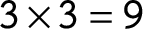 $3\times 3=9$
. Small filters capture fine-grained details, but they are likely to mix up the relevant information from an image with its noise. On the other hand, large filters look for details of a larger size at the cost of a lower specificity. Second, the filter stride is an integer number defining how many pixels the filter will slide through the image. The smaller the stride, the more information from the image that is preserved during the convolution.Footnote
5
Finally, the layer depth defines the number of filters in CONV. Note that all of the filters set by this parameter have the same size.
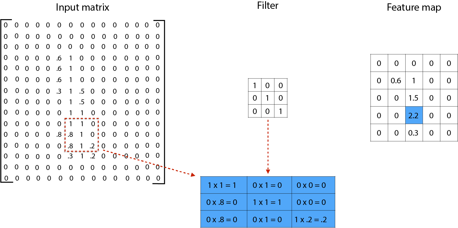
We illustrate how a convolution works in Figure 2. The convolution process involves computing the dot products of the filter and the values of every equivalent pixel space in the image. In this example, the dot product between the entries of the filter and the input of the highlighted image area is
 $2.2$
. Using a stride of 3, the filter slides three steps to the right and again computes the dot product of its entries. The result of this operation is called the feature map, and the convolution process will create as many feature maps as filters specified in CONV.Footnote
6
Illustration of the convolution stage.

Since the resulting feature map is a linear transformation of the input matrix, adding more CONV layers at this point would be redundant; the result could be obtained with a single linear product. Such feature maps are unlikely to produce smooth gradients, a necessary input for the learning phase described in Section 2.3. To address this problem, it is necessary to include an activation or ACT layer. This layer applies a nonlinear transformation to the feature maps before being sent to the next convolution layer. The nonlinearity property allows the network to stack multiple layers and extract more information from the image.
The specific transformation that the ACT layer performs on the input depends on the activation function of the neuron. We briefly describe three of these functions below (Figure A.3 in the online Appendix illustrates their graphic representations). The first one, Sigmoid, is simply the inverse of the logistic function, which bounds the activation values to the
 $[0,1]$
range. A second one is Tahn, a linear transformation of Sigmoid that zero-centers the outputs and bounds them to the
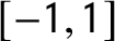 $[-1,1]$
interval. For illustration purposes, we use Tahn for our example in Figure 1. One limitation of the aforementioned functions is that their output becomes flat near their boundaries, limiting the network to learn from inputs with either very low or very high activation values. Addressing these issues, the rectified linear unit (ReLU) is a nonsaturated function that keeps the original input value when it is positive and transforms all negative values to 0.
 $ReLU$
usually increases the learning speed of the network and is now the standard activation function in practice (Nair and Hinton Reference Nair, Hinton, Fürnkranz and Joachims2010).
Given the potentially large size of an image, one of the goals of this stage is to reduce the dimensionality of it while keeping its most relevant information. To reduce the dimensions of the image, it is recommended to include a POOL layer after every CONV
 $\rightarrow $
ACT sequence (Rosebrock Reference Rosebrock2017). The way in which POOL summarizes the information depends on whether it keeps the largest value (max pooling), the smallest value (min pooling), or the average value (mean pooling) of a specific pixel area. In the example of Figure 1, we apply max pooling to keep the largest value from every
 $2\times 2$
pixel area of the matrix. The resulting matrix generalizes the properties of the image, forcing the neural network to pay more attention to whether a feature fits in the image regardless of the location of such a feature.
The CONV
 $\rightarrow $
ACT
 $\rightarrow $
POOL sequence is repeated for each of the filters in the first layer. The resulting feature maps then become the input for the second CONV. This new layer reproduces all of the steps described above, and its filters slide through the feature maps to now look for more complex features, such as a combination of lines or edges. The process is repeated as many times as CONV are in the network.
2.3 Learning
The last stage of the CNN uses the elements extracted during the last CONV
 $\rightarrow $
ACT
 $\rightarrow $
POOL sequence to predict the label of the image. This stage involves a set of fully connected (FC) layers followed by a final ACT, also called output layer, that produces the output value for the prediction. Each neuron in an FC layer receives an input, transforms it, and sends a signal to the neurons to either an additional FC or an ACT layer. The strength of the signal depends on the weight between the emitting and receiving neurons. Positive weights amplify the signals and highlight their contribution to the output. Negative weights, by contrast, weaken the signal to which they are attached.
When the information reaches the output layer, its corresponding nodes deliver the probability that the original input belongs to each label through a given activation function. If the classification task only involves two labels, the output layer estimates the probabilities using an inverse logit. Otherwise, the probabilities are estimated through a softmax layer, the equivalent of a multinomial logistic function. In the example described above, since we want to identify the image from Figure A.1(a) as a digit value, the last layer of our network has 10 neurons or outputs, one for every digit from 0 to 9. Each neuron will provide a probability that the image belongs to each digit, and the model will attach the label with the highest estimated probability.
Until this point, the neural network has performed only a forward propagation—i.e., passing the input data sequentially through each of the layers to generate a prediction. However, for the CNN to learn what features of the image are more likely to belong to each label, it requires a process called backpropagation (Rumelhart, Hinton, and Williams Reference Rumelhart, Hinton and Williams1988). For this operation, the model goes back from the output layer to the input layer with the goal of discovering high-level features of the images. With every step away from the output layer, the model calibrates the weights between neurons to gradually minimize the errors in predictions (Schrodt Reference Schrodt2004; Lucas Reference Lucas2018a). Therefore, the learning process consists of reviewing a set of labeled examples multiple times to find the optimal combination of feature maps and weights that minimize the disparities between true and predicted labels.
We use the loss function to quantify such disparities and as our target for optimization. The smaller the loss, the better the predictions that the classifier is reaching. In more familiar terms, the loss function in an ordinary least squares (OLS) regression is the mean square error, i.e., the mean of the differences between the observed values
 $y_i$
and the predicted values represented by the regression line,
 $\hat {y_i}$
. In the CNN context (and nearly all deep learning applications), the default loss function for binary classification is the binary cross-entropy loss, and for more than two categories the categorical cross-entropy loss.
Analytically, backpropagation searches for the local points in a high-dimensional space where the error derivative of the total loss function is zero. To find those saddle points, the CNN modifies the weights between layers and checks for its resulting changes on the error. This estimation is called gradient descent and consists of repeatedly calculating the slope of each weight with respect to the loss function and modifying such weight to minimize the slope until finally reaching the bottom of the function.Footnote 7
Similar to the previous subsection, we describe the hyperparameters that have to be specified in this stage, and provide recommendations for setting these values in Section 3. First, given the iterative nature of the gradient descent, it is necessary to specify the epochs, or the number of times that all training examples will pass through the network. The model is more likely to fit its weights, as it has more opportunities to review the training examples. It is expected that the prediction errors in the training and validation data will decrease with the number of epochs. However, when the loss in the validity dataset stops decreasing, we should stop the training process (see Section 3.3). In this way, we prevent the model from starting to learn features of the images that are not generalizable outside the training data.
Second, the researcher needs to define the batch size, or the number of training images that need to pass through the network before it updates its weights. If the batch size is equal to the total number of training images, the model will update its weights only after accumulating the prediction errors across all the training images, a task that can demand a lot of computational memory. It also produces a static error surface, where the gradient descent is likely to get stuck in a local minimum. By contrast, the batch size can be equal to one, where the model updates its weights for each training example. Though updating the model with every example decreases the risk of getting stuck on a flat region, it produces a very noisy signal. A middle-way approach splits the training data into mini-batches, allowing the model to update its parameters several times during an epoch.Footnote 8
Finally, we can specify the learning rate, or the size and timing of the steps we take to reach the function’s local minimum. Finding the optimal learning rate in advance presents a conundrum. A large learning rate will jump around the function, overshooting its minimum. By contrast, a very small learning rate is more likely to find a local minimum, but it will take a long time to converge. Ideally, we would use a learning rate that helps the model to start exploring the entire hyperparameter space and to approach the global minimum by gradually making smaller jumps (Buduma and Locascio Reference Buduma and Locascio2017). Yet it is hard to know ex ante when and by how much to decrease the learning rate along the iterations. Moreover, having a unique learning rate to estimate all the parameters could hinder the model to explore the entire space in an efficient way. Fortunately, the researcher can choose from different gradient descent optimization algorithms that lead to faster convergence and that do not require to manually tune up the learning rate.Footnote 9 For example, the adaptive gradient algorithm (Adagrad) adjusts the learning rate to each parameter, computing smaller updates for frequently occurring features and larger updates for the less frequent ones. The adaptive moment estimation (Adam) follows the same logic as Adagrad, but it solves the radically diminishing learning rate of the latter (Ruder Reference Ruder2017). That advantage makes it the current default choice in machine learning.
3 Practical Recommendations
In this section, we present and discuss some guidelines to reach and improve the decisions researchers will have to make when implementing their own CNN, as well as a set of common practices and “rules of thumb” for different cases.
3.1 Building a CNN Architecture
The simplest structure in a CNN includes a single CONV with a unique filter followed by an ACT and a POOL layer, and a single FC with a subsequent ACT that makes the prediction. We can represent more complicated architectures with the following pattern:

where M and K are the number of times that a given sequence is repeated. For example, the simplest structure mentioned above will have
 $M=K=1$
.
We can change the complexity of the structure in two ways. First, we can make a deeper network by increasing either M or K. The former option implies adding more CONV to the network. The deeper a network is, the more complex the features from the image that the convolutional layers will find. We expect a larger M in models using extensive training data and a complex classification goal. Alternatively, we can deepen the network by increasing K, or the number of FC layers toward the end of the network, allowing for a more complex classifier.
Another element that can vary from architecture to architecture is the inclusion of a POOL layer (therefore, the “?” sign next to POOL in the pattern above). While some models rely on convolutional layers with longer strides to reduce the dimensionality of the data, others use POOL layers that simplify the data between each round of convolutions. Including this type of layers allows the network to deal with simpler data, but also forces it to focus on less specific features of the images. At the end, this step “compresses” the amount of information from which the model learns.
There is not a unique recipe for the values of these hyperparameters. As a starting point, basic structures include
 $ 1 \leq M \leq 3$
, and
 $K \geq 1$
(Rosebrock Reference Rosebrock2017). But researchers should consider the size of their data, the number of desired output labels, the similarity between output labels, and the intraclass variance (i.e., how dissimilar are the objects belonging to the same label). We also encourage the reader to experiment with different settings to test the model performance using hyperparameter grid search (see Section 5).
The number and size of the filters in each CONV are other relevant hyperparameters to consider. Here, we go back to the importance of fully knowing the data under analysis to inform that decision. A higher number of filters will make the network look for more features of the image sharing a similar level of complexity. A common procedure to set this number involves increasing the number of filters gradually through the network. Some scholars recommend to double the number of filters every time we add an additional CONV (Shang et al. Reference Shang, Sohn, Almeida and Lee2016). Other architectures present even larger increments.Footnote 10
With regards to the filter size, if the pixel space is sufficiently large and the model’s goal is to find large-scale features of the image, filters of size
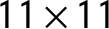 $11\times 11$
or
 $9\times 9$
would be fitting. However, if the features that distinguish the images are more fine-grained, then small filters (
 $3\times 3$
or
 $5\times 5$
) will be more appropriate. For example, Han et al. (Reference Han2018) find that detecting whether a person is smiling in a picture relies on broader and more evident identification of features like the strong curvature of the lips that are easily captured with larger filters. In contrast, detecting whether a person is frowning relies on finding light wrinkles in the forehead, a feature that is more efficiently identified with a smaller kernel.
The last considerations have to do with the characteristics of POOL. In very complex networks, pooling generally uses
 $3\times 3$
receptive fields in the early stages of the model to then reduce its size to
 $2\times 2$
. Simpler networks use
 $2\times 2$
receptive fields and a stride of 2 all along its sequence. Finally, while max pooling is the most common pooling layer (Ranzato, Boureau, and Cun Reference Ranzato, Boureau and Cun2008; Boureau, Ponce, and LeCun Reference Boureau, Ponce and LeCun2010), recent findings suggest that some hybrid pooling methods, such as the “mixed max-averaging pooling,” can also improve performance for an extra computational cost (Lee, Gallagher, and Tu Reference Lee, Gallagher and Tu2016).
3.2 Software
There are multiple open-source machine learning packages that researchers can use to design and run a CNN. Some of the most popular are TensorFlow (from Google), Caffe (from UC Berkeley), CNTK (from Microsoft), PyTorch (from Facebook), and MXNet (supported by AWS). Keras is a neural networks API written in Python that supports models like CNNs and recurrent networks, and that a very accessible, efficient, and user-friendly interaction with packages like TensorFlow.
The differences between the aforementioned packages are in terms of speed, energy efficiency, and accessibility. As a quick summary, TensorFlow is faster when running large-scale models, while Caffe is faster with small-scale ones (assuming they are both implemented on a CPU-based platform). Furthermore, while PyTorch is more memory efficient than its counterparts, MXNet requires the least amount of computational energy. Thus, scholars should consider the size and complexity of their data and classification objectives, plus the hardware/computational resources they have at hand. Zhang, Wang, and Shi (Reference Zhang, Wang and Shi2018) offer a great compilation of insights regarding the performance of these packages with respect to speed, memory, and energy.
Beyond these packages, there are other tools that facilitate the design of the architecture of a CNN and also allow researchers to take advantage of pretrained models. In particular, these might be interesting for deep learning beginners or scholars with less advanced programming skills. The options include but are not limited to Amazon AWS Machine Learning Training, Google Cloud AutoML, or Google Cloud Machine Learning Engine. For a review of these platforms and their performance, see Webb Williams (Reference Webb Williams2019).
3.3 Finding the Right Amount of Training
As with any human-performed task, prediction accuracy for a CNN model comes only with practice. A model requires to be trained over multiple iterations, so it can learn the relevant patterns in the training data. Not doing so leads to underfitting, which occurs when the model is too simple to account for all the variance across images. An underfitted model makes strong assumptions when classifying the data, leading to a high bias on its predictions. As we increase the number of training iterations, the model can continue learning the general patters of the training examples and adjust its filter weights accordingly.
On the other hand, training the model for too many iterations will eventually lead to overfitting. This works against generalization, a principle in machine learning that refers to the performance of the model with examples outside the training set. When overfitting occurs, the model starts picking up noise or random fluctuations from the training images as valuable concepts for classification. To check for overfitting, we can monitor model performance in the training and validity sets after each epoch and stop when the loss decreases (or the model’s accuracy no longer increases) in the validity data. Preventing overfitting while allowing the model to learn the most relevant features of the images is a practical dilemma, and it depends not only on the number of training iterations but also on the model architecture. We suggest below a few ways to optimize the training.
3.3.1 Increase the Size of the Training Set
This is the default solution. The more images in the training set, the more opportunities the model has to distinguish the systematic patterns across images from random fluctuations. If getting more training data is difficult, researchers can artificially increase the size of the training set using data augmentation (see Section 3.4.4).
3.3.2 Explore Different Network Structures
Overfitting can be the result of a very complex model with too many features. We can try removing certain features of the model and compare its performance. However, as mentioned above, we must be aware that taking away too many parameters can lead to a very rigid model. The problem is then knowing how many and which of these parameters we should remove. One way to answer this question involves using a grid search. This technique runs the model in a “for-loop,” compiling it with a different set of hyperparameters in each iteration. The results allow the researcher to compare the performance of multiple settings and to choose the configuration with the lowest loss.Footnote 11
3.3.3 L1 and L2 Regularization
Overfitting often produces model weights with very large values. We can mitigate this problem using regularization, a technique that forces the model to take only small weight values. The most common regularization techniques increase the costs associated with the weights. The Least Absolute Shrinkage and Selection Operator (Lasso Regression or L1), for example, penalizes large values by adding the absolute value of the weights to the loss function. Such penalization encourages the model to have as many weights closer to 0 as possible, removing some of the features for the classification. The Ridge Regression (L2), in contrast, penalizes large values by adding the square magnitude of the weights to the loss function. In this case, this regularization overpenalizes very large weights, but it will not dismiss as many features as L1. The technical details for both types of regularization are in the Glossary.
3.3.4 Dropout
This is another regularization technique that, as its name suggests, randomly “drops out” a set of neuron activations at each iteration of the training (Srivastava et al. Reference Srivastava, Hinton, Krizhevsky, Sutskever and Salakhutdinov2014). By ignoring some of the information that passes across layers, this approach slows down the learning for each training iteration, forcing the model to learn more robust features that activate multiple neurons. Dropout is typically applied in between FC layers with a dropout probability of no more than 50%. Some researchers also suggest adding this operation with small probabilities (between 10% and 25%) between CONV layers (Rosebrock Reference Rosebrock2017).
3.4 Optimizing Your Training Set
A better learning depends not only on the number of times the model can learn from the examples, but also on the information it extracts from them. We suggest four concepts to keep in mind when choosing the amount and quantity of data that the model will learn from.
3.4.1 Active Learning
We recommend picking the most useful instances of each class to train the model (Settles Reference Settles2009; Miller, Linder, and Mebane Reference Miller, Linder and Mebane2020). This suggestion is particularly convenient when obtaining additional training examples is a difficult, time-consuming, or expensive task. Selecting those examples should be based on two goals: informativeness (i.e., how much the instances help the classifier to improve its performance) and representativeness (i.e., how well the instances represent the overall input patterns of the entire dataset). Both are rarely achieved simultaneously, and researchers must often choose which one to prioritize at the cost of the other (Huang, Jin, and Zhou Reference Huang, Jin and Zhou2014).
3.4.2 Class Balance
It is also useful to make sure that all classes in the training set are represented by a similar number of examples (Buda, Maki, and Mazurowski Reference Buda, Maki and Mazurowski2018). Class balance prevents skewing the model’s predictions toward the label with more training instances (Japkowicz and Stepehn Reference Japkowicz and Stepehn2002). This is a recurrent issue in situations where the positive cases represent a minority of all the cases, such as locating oil-spills (Kubat, Holte, and Matwin Reference Kubat, Holte and Matwin1998) or identifying fraudulent bank operations (Chan and Stolf Reference Chan and Stolf1998).
3.4.3 Image Cleaning
Another risk when training a model is that it may learn visual features that are alien to those defining the categories of interest (e.g., ink stains that are not relevant to the content of a document). As described above, images should be preprocessed to make sure they appear as similar as possible. In some cases, this step may require modifying and cropping irrelevant parts of the image.
It is also possible to homogenize the data of every training batch. In this case, batch normalization transforms the outputs of the convolutional layers to parameters with zero mean/unit variance, allowing the layer activations to be appropriately handled by any optimization method (Ioffe and Szagedy Reference Ioffe and Szagedy2015). This technique keeps the network from focusing on outlying activations that decelerate its learning.
3.4.4 Data Augmentation
This technique produces random variations of the original training images by, for example, flipping, flopping, rotating, zooming out, or combining all of these alternatives (Chatfield et al. Reference Chatfield, Simonyan, Vedaldi and Zisserman2014). The augmented cases will force the model to pay less attention to the specific location and orientation of a feature in an image and instead grasp its relationship to other image features.
3.5 Transfer Learning
Training the model from scratch can be computationally expensive and requires a large dataset to avoid overfitting. An alternative approach involves transfer learning, where an already trained model can be directly applied to a new task or used as the starting point for training a new model (Pan and Yang Reference Pan and Yang2010). Transfer learning is an available resource when the researcher is lucky enough to find a model already trained on a dataset with similar content to hers, and that also performs a similar classification task.
To adapt the trained model to the new data, we can deactivate (or “freeze”) its initial layers. This way the model takes the weights previously learned and calibrates their values based on the new target categories. For example, Zhang and Pan (Reference Zhang and Pan2019) used transfer learning to fine-tune VGGNet, a canonical CNN model trained on a set of 1.2 million images, to identify collective action events. Because those categories do not cover human faces or crowds, crucial elements of protests and demonstrations, the authors “froze” the first 12 layers of a VGGNet and retrained the last four layers with a set of images containing their target elements.
In Table A.1 in the online Appendix, we provide a summary of popular architectures that can serve as the basis for transfer learning. We include technical details such as the number of layers and size, performance indicators, and the references to the articles that introduced them. See also Webb Williams et al. (Reference Webb Williams, Casas and Wilkerson2020) for a detailed explanation of this method, as well as some resources available when using this approach.
3.6 Validate and Check the Results
Similar to textual analysis, a key principle of machine-coded visual analysis is “validate, validate, validate” (Grimmer and Stewart Reference Grimmer and Stewart2013, 269). Validating the results will reveal potential sources of errors and provide information about the model fit. An insightful way to improve the model is to review the misclassified images in the validity set. As we will show in the example below, this is a helpful practice to find potential problems in the model. Another way to check the validity of the model’s predictions is to visualize the most relevant features driving the predictions (Zeiler and Fergus Reference Zeiler and Fergus2014; Won et al. Reference Won, Steinert-Threlkeld and Joo2017). Similar to finding the most important coefficients in a regression, this exercise provides information about the mechanisms behind the predictions. For example, some of these tools provide “maps” that reveal what parts of the image or specific features were most determinant in reaching a prediction. This in turn can provide the researcher with information to help complement or tune the samples included in the training pool.
4 A Warning Note: The Limits of CNNs
Throughout this article, we present the functioning and components of CNNs, as well as an illustration of their applicability to data collection for social science purposes. However, below we also mention some of the most important flaws of CNNs that researchers must keep in mind when solving complex tasks with this tool.
First, CNNs do not account for the orientation of objects in a picture. While they are robust against small-scale deformations, their final representations are not geometrically invariant (Ciresan et al. Reference Ciresan, Meier, Masci, Gambardella and Schmidhuber2011; Gong et al. Reference Gong, Wang, Guo and Lazebnik2014). Ideally, we would like CNNs to identify an object regardless of its size or rotation. A CNN will identify a face when it finds features associated with an eye, a nose, and a mouth, ignoring whether the eyes are below the nose and above the mouth, for example. This problem stems from the fact that the model focuses on routing the pixel information throughout the layers without adding any information about the relative position of the extracted features. Without a comprehensive and extensive training dataset (see Section 3.4.4), the classification of pictures becomes inaccurate and subject to error, even in cases involving simple tasks (Sabour et al. Reference Sabour, Frosst and Hinton2017).
Another criticism of CNNs lies in their lack of uncertainty measures. Unlike traditional models such as regression, these tools do not yield quantities like standard errors that aid with inferences or assessments of confidence. While the last layers of the CNN provide the “probabilities” of an image belonging to a certain class, these quantities should be used with caution. Recent evidence shows that seemingly imperceptible alterations to an image can cause drastic changes in the outcome probabilities (Nguyen et al. Reference Nguyen, Yosinski and Clune2015). This research implies that the likelihood for an image to be identified a certain way might depend not only on its basic features, but also on stochastic aspects, such as its illumination or the proportion of a picture it occupies.
Finally, CNNs cannot discover latent dimensions or classify abstract concepts. As a rule of thumb, if a human cannot validate a trait, a CNN will not be able to do it, either. Recall that some inputs that give context to a visual message, such as positions, get lost during the classification process, and that certain perturbations that would not mislead humans can have a significant impact on the CNN output (Gong et al. Reference Gong, Wang, Guo and Lazebnik2014; Goodfellow et al. Reference Goodfellow, Bengio and Courville2016). Moreover, other visual messages are filtered through cognitive biases, experiences, and backgrounds of the person consuming them. A CNN relies on factual features and unambiguous labels to learn the association between them. Thus, abstract concepts or latent traits, such as the emotions that images trigger or evoke, offer a hard case not only for the actual classification process (Casas and Webb Williams Reference Casas and Webb Williams2019), but also for the postclassification analysis and validation of the results. In these cases, the risk of incurring in post hoc interpretations of the outcomes is high given the flexibility to adapt the outputs to the researcher’s expectations.
In summary, researchers need to be aware of the limitations of CNNs, cautious about the objectives they expect CNNs to fulfill, fully knowledgeable of the data under analysis and training, and careful about their interpretation of the outputs of the CNN.
5 Application: Coding Electoral Results from Vote Tallies
We illustrate the implementation of a CNN by extracting information from vote tallies of Mexico’s 2015 federal election. We chose this case for two main reasons. First, the task of “handwritten classification” is a text book application of CNNs in the field of computer science due to its objective nature and low dimensionality. For the specific case of coding vote returns, handwritten numbers have one color channel and a low number of features and variations, which allows us to represent the numbers in a straightforward way. Moreover, we expect that a number “8,” for example, will be always coded as such regardless of the coder.
Second, this example demonstrates the benefits of visual analysis to scholars and policy practitioners. We think the adequate use of CNNs may be a useful tool for scholars working with different types of archival data (Coüasnon, Camillerapp, and Leplumey Reference Coüasnon, Camillerapp and Leplumey2007; Lladós et al. Reference Lladós, Pratim-Roy, Rodríguez and Sánchez2007; Taylor Reference Taylor2008; Homola Reference Homola2018; Huff Reference Huff2018). At the same time, it proposes a transparent, cost-efficient mechanism to record the information from hand-counted vote tallies, a prevalent document in most national elections. The technology can help election administrators to reduce the number of accidental errors during the hand-counting process, a problem that occurs in almost 40% of the Mexican vote tallies (Challú, Seira, and Simpser Reference Challú, Seira and Simpser2020). Moreover, this technology can shorten the waiting time for the announcement of the results, a period of distress for candidates and voters in elections across the world.Footnote 12
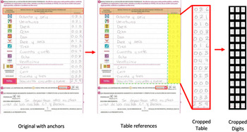
Figure 3 shows an example of the handwritten numbers in one of the tallies in our database. To first extract the handwritten digits, we designed a function that uses the coordinates of three focal points in the tally as anchors to crop first the table with the vote counts and then each of the individual digits in it.Footnote 13 Once we extracted the digits from the tallies, we built our training, validation, and test sets of size 24,271, 2,000 and 2,616, respectively. The target sample has 23,058 digits from one specific district in the country.
Example of the image of a tally.

To illustrate the process of finding the “best model” for our data, we proceed in three steps. First, we use an already trained model for reading handwritten numbers of the Modified National Institute of Standards and Technology’s (MNIST) database (LeCun et al. Reference LeCun1989) and test its accuracy on our database. Second, we fine-tuned the model using a hyperparameter grid search. Finally, we used transfer learning to allow the model to learn the particular characteristics of our data. The description of each of the steps below aims to be a template for researchers interested in designing and tuning their own models.
We start using a base model with two convolutional layers, each followed by a max pooling layer, and three fully connected layers that precede the softmax activation layer. Figure A.4 in the online Appendix presents the detailed architecture.Footnote 14 This stage involves training the model using exclusively examples from the MNIST dataset, out of which 60,000 handwritten digits are in the training set, and 10,000 different examples will constitute the validity set.
While the base model achieves high levels of accuracy on the MNIST digits (0.9914), we want to know how useful this model is to predict the digits from the tallies. Initially, the results are not very encouraging: the accuracy rate of this model in our validation dataset is only 0.3245. We interpret the significant drop in the accuracy rate as a result of the specific nature of our data. Most of the digits from the tallies are less defined and have a wider range of pixel intensities than those in the MNIST dataset. Moreover, the digits from the tallies have bounding boxes, stains, and pencils marks, and other elements alien to the actual numbers (see Figure A.7 in the online Appendix as an example).
A first step to improve the performance of the base model is to tune some of its hyperparameters by using grid search. This method identifies which settings lead to the best performance (in our case, accuracy in the validation sample). We ran several iterations of the model, each of them combining different values of the following hyperparameters: number of convolutional layers, number of filters in each layer, dropout rate, size of the fully connected layers, and number of epochs. Every specific setting starts training the model from scratch using the 60,000 examples from the MNIST dataset and evaluates its performance on the digits from the tallies. Table A.3 in the online Appendix shows several examples of these model options and their respective accuracy.
After testing different hyperparameter settings, our fine-tuned model contains three convolutional layers (with 32, 32 and 112 filters of size 3
 $\times $
3, respectively), a dropout rate of 0.2, and denser fully connected layers (with 110 and 30 nodes, respectively). Figure A.5 in the online Appendix details the architecture and characteristics of this network. We also found the optimal amount of training after 45 epochs. The accuracy of the fine-tuned model on our validation data is 0.3720, almost 0.0475 higher than the base model. While this is an important gain in accuracy, we still want to achieve higher levels.
Thus, the next step uses transfer learning (see Section 3.5) in order to improve the classification. This step involves retraining the model using now the 24,271 labeled digits from the tallies and freezing the first convolutional layer of the fine-tuned model. “Freezing” the first layer implies that we load the weights found by the fine-tuned model using only MNIST digits as training data. We perform data augmentation on the training set comprised of digits from real-world tallies. This approach significantly improves the model performance on the prediction of digits from tallies: the accuracy scores in the validation and test sets are 0.9495 and 0.9659, respectively.Footnote 15
Finally, we checked and tried to interpret the reasons behind the model errors. In this case, many misclassified examples are digits misplaced outside the guiding box (see, e.g., Figure A.8 in the online Appendix). Other mistakes were due to almost illegible numbers or specific handwriting styles that confounded “4” for “9.” As explained in Section 3, these examples spotlight the importance of the postclassification process to understand the sources of errors, identify problematic cases, and conduct parameter tuning. Such a process requires humans actively finding out the sources of error in the model and correcting the most important mistakes. With this example we want to stress that using CNNs to classify images should not eliminate human intervention, but should rather limit it to the most crucial or controversial decisions.
To check the general validity of the model predictions, we calculate the parties’ vote total in Mexico City’s #15 Congressional district. The digits from the tallies of this district form our target sample.Footnote 16 Since all the vote counts have three digits, including leading zeros, we estimate the “uncertainty” around a prediction with a weighted average of the label probabilities for each digit in the vote count. This weighted mean assigns more importance to the errors that happen in the hundreds than in the tens or units. For example, if the model mislabels a “9” for a “4,” the bias in the vote count would be larger when the vote count is “931” (underestimating the vote count by 500 votes) than when it is “139” (when the bias would be of only 5 votes).Footnote 17 Once we compute the weighted mean of all the vote counts per tally, we label those with a mean larger than 0.9 as “high quality.”
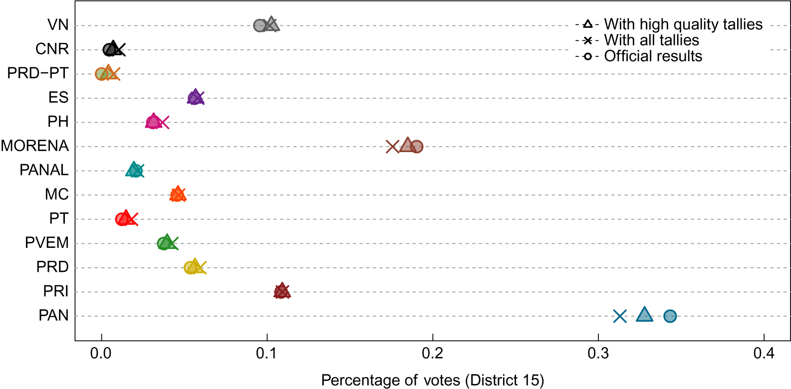
Figure 4 compares the estimated vote shares for each party (crosses for all tallies; triangles for “high quality” tallies) with those reported by the electoral authority (circles).Footnote 18 As the plot shows, the CNN recovers proportions similar to the official ones, and this performance improves when using high quality tallies. Overall, the method is able to correctly identify the ranking and magnitude of vote counts. This accurate identification illustrates the applicability of CNNs and their power for data collection tasks.
Vote proportions by party in District 15: official vs. predicted.

The example above illustrates the usefulness of CNNs to extract information from large pools of images in an efficient, fast, and reliable way. At the same time, this example also acknowledges the limitations of CNNs when it comes to completing certain tasks.
6 Conclusion
Using computer vision techniques for image retrieval and classification can extend the scope of the data, theory, and implications underlying the study of several social phenomena. In this paper, we presented a comprehensive guide for researchers interested in using CNNs for visual content coding and classification. We presented the intuition behind CNNs, highlighted their potential, and described their structure and implementation.
CNNs have a wide variety of applications in multiple fields of the social sciences. They can be applied to similar data collection problems like the one outlined in the text: retrieving signatures or the votes that were whipped for a given policy registered in historic documents, classifying written notes, or even the extraction and interpretation of symbols. They can also be applied to the coding of more complex political phenomena. Examples may include identifying the sentiment of material from electoral campaigns (Lucas Reference Lucas2018b), recording the activities of crowds in a protest (Won et al. Reference Won, Steinert-Threlkeld and Joo2017; Zhang and Pan Reference Zhang and Pan2019), counting the number of people waiting to vote in polling stations (Stein et al. Reference Stein2020), measuring social polarization (Dietrich Reference Dietrich2020), assessing media bias in the photographic coverage of candidates (Neumann Reference Neumann2019), or detecting the demographic composition of a neighborhood (Wilcox-Archuleta Reference Wilcox-Archuleta2019). In an era where pictures and videos have an increasing role in shaping public opinion, elite decisions and political dynamics, the extraction of information from images and visual content invite a wider variety of relevant questions.
In this article, we outlined the structure, functioning, and implementation of CNNs with the objective of making the tool more accessible to social scientists interested in using visual content to address such questions. With the application of a CNN to code information from vote tallies, we also illustrate the challenges that the “real-world” data in which we are interested pose to standard and well-tested models in computer science. We also provide a list of practical recommendations and advice that we hope will help social scientists to immerse in the field of deep learning and CNNs.
The study of new data sources both complements and enhances the knowledge that we already have about the political world. However, these opportunities should be paired with a deep understanding of the characteristics, mechanisms, and consequences of tools like CNNs. Our intention is to illustrate the benefits and substantive impact of CNNs for social scientists, but also to present some of the challenges and practical issues that researchers should consider when dealing with visual data. Our hope is that this article encourages scholars to use CNNs in their own analyses while avoiding the most common misunderstandings and pitfalls of this tool.
Data Availability Statement
Replication code for this article has been published in Code Ocean, a computational reproducibility platform that enables users to run the code and can be viewed interactively at Cantú and Torres (Reference Cantú and Torres2020a) at https://doi.org/10.24433/CO.3401138.v1. A preservation copy of the same code and data can also be accessed via Dataverse at Cantú and Torres (Reference Cantú and Torres2020b) at https://doi.org/10.7910/DVN/UNYOLF.
Supplementary Material
For supplementary material accompanying this paper, please visit https://doi.org/10.1017/pan.2021.9.