





1. Introduction
One of the critical areas for the success of fusion reactors is our ability to confine alpha particles long enough for them to transfer most of their energy to the bulk plasma. Losing too much energy from fusion born alphas would decrease the efficiency of future plants and harm the integrity of its plasma facing components. Although experiments with energetic particles from neutral beam injection and ion cyclotron resonance heating have been carried out, their spatial localisation and velocity space anisotropy differ from fusion born alphas (Fasoli et al. Reference Fasoli2007; Gorelenkov, Pinches & Toi Reference Gorelenkov, Pinches and Toi2014). While experiments producing alpha particles have been performed, their regime is still quite far from burning plasma conditions (Villari et al. Reference Villari2025). It is therefore necessary to continue developing models to study the dynamics of alpha particles in magnetically confined fusion devices.
In recent years, quasisymmetric (QS) stellarators have become a highly promising configuration for future reactors. New optimisation schemes have made it possible to find QS configurations with error fields down to geomagnetic field levels (Landreman
 $\&$
Paul Reference Landreman, Buller and Drevlak2022). These configurations can reduce non-turbulent transport to acceptable neoclassical levels, and have flexibility to optimise turbulent transport. At the same time, test particle guiding centre collisionless and collisional alpha losses have been successfully reduced in highly optimised configurations (Landreman, Buller & Drevlak Reference Landreman, Buller and Drevlak2022). However, numerical simulations typically examine the full alpha distribution function to determine prompt losses without resolving the fine scale velocity and position space features of the collisional boundary layers associated with resonances and the narrower collisional boundary layer surrounding the separatrices of any island structures (Bader et al. Reference Bader, Anderson, Drevlak, Faber, Hegna, Henneberg, Landreman, Schmitt, Suzuki and Ware2021; Lazerson et al. Reference Lazerson, LeViness and Lion2021). Resonant particles are very sensitive to collisions, causing non-negligible transport of passing as well as trapped alphas in the presence of departures from quasisymmetry (Catto, Tolman & Parra Reference Catto, Tolman and Parra2023; Catto Reference Catto2025). A detailed numerical evaluation of the pitch angle scattering of alphas in and out of the collisional resonant region is required to perform the radial flux integrals over many neighbouring flux surfaces. The resonant pitch angle changes with radius so the radial extent of the loss region can be substantial. In some configurations, it may not extend to the last closed flux surface which codes may focus on for fixed background plasma density and ion temperature profiles. In addition, once built, these devices will likely have higher error fields than ideally optimised configurations.
Boundary layers appear in several contexts (Bender & Orszag Reference Bender and Orszag1999). In drift kinetic transport, collisional boundary layers are relevant in neoclassical transport (Calvo et al. Reference Calvo, Parra, Velasco and Alonso2017) and trapped alpha particle resonant transport due to magnetic field errors in tokamaks (Catto Reference Catto2019) and QS stellarators (Catto et al. Reference Catto, Tolman and Parra2023). Tolman & Catto (Reference Tolman and Catto2021) also show possible trapped particle transport in the presence of time dependent perturbations with an effective Krook collision operator for an axisymmetric configuration. In this work, we evaluate the resonant energy transport of passing alpha particles in the presence of steady state deviations from quasisymmetry in magnitude and field direction. Stellarator optimisation schemes normally focus on the trapped particles because the passing particles are viewed as well confined as they normally trace out flux or drift surfaces to lowest order. However, in the presence of a resonance this is no longer possible. Collisions are required to prevent singular behaviour, and radial transport occurs. In a stellarator the passing alpha particles are sensitive to a change in the direction of the magnetic field and typically have a resonance very near to a rational surface as demonstrated herein. To resolve the collisional boundary layer that forms around resonances with these perturbations, we use the diffusive pitch angle scattering term due to alpha collisions with the background ions from the collision operator.
We first formulate a drift kinetic treatment of alpha particles. For passing alphas, the resonance between the parallel streaming and the tangential drift terms leads to the formation of a collisional boundary layer where the effective collision frequency is enhanced and a well behaved perturbed distribution function exists. These particles are sensitive to collisions and can cause substantial radial transport. By working in an appropriate set of coordinates and trajectory averaging along the streaming variable, we arrive at a 1D equation in pitch angle. This allows us to calculate the perturbed distribution function, which we input into the quasilinear flux expression obtained from the lowest order drift kinetic equation to get the radial energy flux and diffusivity. The alpha energy diffusivity allows us to assess potential particle and energy loss and estimate the model limitations.
In § 2 we describe the applied background magnetic field and spatial coordinates, and the deviation from quasisymmetry. In § 3 the model is introduced, including the lowest and first order equations, the solution to the perturbed distribution function and its resulting energy transport. In § 4 phenomenological estimates are included, which provide physical intuition into collisional boundary layers, and an explanation of the limitations of the model is presented. Section 5 shows the evaluation of the resulting transport, along with a study of the model limitations and a sensitivity analysis of the key parameters. In § 6 the results are discussed, including some insights for stellarator design and conclusions. In the appendices, we discuss the barely passing asymptotic limit and the agreement with previous results, provide some additional mathematical details and include a more detailed discussion on the model limitations.
2. Magnetic field description
2.1. Background magnetic field
A general stellarator magnetic field with well defined nested flux surfaces can be described by (Boozer Reference Boozer1981)
 \begin{align} \boldsymbol{B} = B\,\boldsymbol{b} = \boldsymbol{\nabla }\alpha \times \boldsymbol{\nabla }\psi _p = K\,\boldsymbol{\nabla }\psi _p + G\,\boldsymbol{\nabla }\vartheta + I\,\boldsymbol{\nabla }\zeta , \end{align}
where
 $\vartheta$
is the poloidal angle and
 $\zeta$
is the toroidal angle. The poloidal flux function
 $\psi _p$
, defined by
 $2\pi \psi _p = \int _{\mathrm{pol}} d^{2}\boldsymbol{r}\boldsymbol{\cdot }\boldsymbol{B}$
, labels the magnetic surfaces, and along with
 $\alpha \equiv \zeta - q(\psi _p)\,\vartheta$
, defines the magnetic field lines in every flux surface. The safety factor
 $q ={\boldsymbol{B}\boldsymbol{\cdot }\boldsymbol{\nabla }\zeta }/{\boldsymbol{B}\boldsymbol{\cdot }\boldsymbol{\nabla }\vartheta }$
has been defined to be a flux function, and the rotational transform is
 $\text{-}{\kern-2.5pt}\iota = q^{-1}$
. The coefficients
 $G$
and
 $I$
are defined as the toroidal and poloidal currents, as in Landreman & Catto (Reference Landreman and Catto2012),
 \begin{align} \int _{\mathrm{tor}} d^{2}\boldsymbol{r}\boldsymbol{\cdot }\boldsymbol{J} = \frac {cG}{4\pi }\int _{-\pi }^{\pi } {\rm d}\boldsymbol{r}\boldsymbol{\cdot }\boldsymbol{\nabla }\vartheta = \frac {cG}{2}, \end{align}
 \begin{align} \int _{\mathrm{pol}} d^{2}\boldsymbol{r}\boldsymbol{\cdot }\boldsymbol{J} = \frac {cI}{4\pi }\int _{0}^{2\pi } {\rm d}\boldsymbol{r}\boldsymbol{\cdot }\boldsymbol{\nabla }\zeta = \frac {cI}{2}, \end{align}
where
 $\boldsymbol{J}$
is the current density and
 $c$
is the speed of light. The definition of
 $\boldsymbol{B}$
gives
 $\boldsymbol{B} \boldsymbol{\cdot }\boldsymbol{\nabla }\psi _{p} = 0 = \boldsymbol{B} \boldsymbol{\cdot }\boldsymbol{\nabla }\alpha$
. Forming the product of the second and third forms of
 $\boldsymbol{B}$
in (2.1) we calculate the inverse of the Jacobian of the set of coordinates
 $(\psi _{p},\vartheta ,\zeta )$
,
 \begin{align} \boldsymbol{\nabla }\psi _p \times \boldsymbol{\nabla }\vartheta \,\boldsymbol{\cdot }\, \boldsymbol{\nabla }\zeta = \boldsymbol{B}\boldsymbol{\cdot }\boldsymbol{\nabla }\vartheta = q^{-1}\,\boldsymbol{B}\boldsymbol{\cdot }\boldsymbol{\nabla }\zeta = {B^{2}}/{(q\kern-1.3pt I + G)}. \end{align}
From pressure balance
 $\boldsymbol{J}\times \boldsymbol{B}=c\boldsymbol{\nabla }p(\psi _p)$
, where
 $p$
is the total pressure, the radial current
 $\boldsymbol{J}\boldsymbol{\cdot }\boldsymbol{\nabla }\psi _p$
has to vanish, giving
 $\boldsymbol{\nabla }\boldsymbol{\cdot }(\boldsymbol{B}\times \boldsymbol{\nabla }\psi _p)=0$
. This condition forces the coefficients in
 $\boldsymbol{B}$
to satisfy
 $\partial\kern-1pt I/\partial \vartheta =\partial G/\partial \zeta$
and therefore
 ${\partial }(\oint {\rm d}\zeta \,I)/{\partial \vartheta } = 0 = {\partial }(\oint {\rm d}\vartheta \,G)/{\partial \zeta }$
. Consequently, this suggests working in Boozer coordinates with
 $I=I(\psi _p)$
and
 $G=G(\psi _p)$
flux functions (Boozer Reference Boozer1981) and the Jacobian’s angular dependence that of
 $B^2$
. Hence, the Lagrangian of the motion of charged particles in this field will inherit the angular dependence of
 $B^2$
. In an ideal QS stellarator field there is an angular coordinate that
 $B=|\boldsymbol{B}|$
does not depend on, implying by Noether’s theorem (Noether Reference Noether1918) that we will be able to define a conserved canonical momentum. Satisfying this property, as in axisymmetric fields, ensures the collisionless confinement of particles in a more general class of configurations, known as QS stellarators.
2.2. Spatial coordinates
We work in a QS configuration with QS poloidal and toroidal numbers
 $M$
and
 $N$
positive integers. The magnetic field magnitude on a flux surface only depends on a single periodic angle variable (Nührenberg
 $\&$
Zille Reference Nührenberg and Zille1988; Boozer Reference Boozer1995)
 \begin{align} \eta = M\vartheta - N\zeta . \end{align}
To take advantage of the symmetries of the problem, it is often convenient to work with the angular variables
 $\eta ,\alpha$
instead of the Boozer angles
 $\vartheta ,\zeta$
. They relate to each other as
 \begin{align} \vartheta = {(N\alpha + \eta )}/{(M - qN)}, \end{align}
 \begin{align} \zeta = {(M\alpha + q\eta )}/{(M - qN)}. \end{align}
In the set of coordinates
 $(\psi _p,\eta ,\alpha )$
the inverse of the Jacobian becomes
 \begin{align} \boldsymbol{\nabla }\psi _p \times \boldsymbol{\nabla }\eta \boldsymbol{\cdot }\boldsymbol{\nabla }\alpha = \boldsymbol{B}\boldsymbol{\cdot }\boldsymbol{\nabla }\eta = (M - qN)\,\boldsymbol{B}\boldsymbol{\cdot }\boldsymbol{\nabla }\vartheta = (M - qN)\,B^{2}/(q\kern-1.3pt I + G) . \end{align}
In the radial direction, we define the toroidal flux function
 $\psi _t$
as
 $2\pi \psi _t =$
 $\int _{\mathrm{tor}} d^{2}\boldsymbol{r}\boldsymbol{\cdot }\boldsymbol{B}$
, which satisfies
 $\partial \psi _{t} / \partial \psi _{p} = q(\psi _{p})$
, and the helical flux function as
 \begin{align} \psi _{h} = M\psi _{p}-N\psi _{t}. \end{align}
Differentiating (2.9) we get
 ${\rm d}\psi _h = (M - qN)\, {\rm d}\psi _p$
, and therefore the inverse of the Jacobian of the set of coordinates
 $\boldsymbol{\nabla }\psi _h \times \boldsymbol{\nabla }\eta \boldsymbol{\cdot }\boldsymbol{\nabla }\alpha = (M - qN)\,\boldsymbol{B}\boldsymbol{\cdot }\boldsymbol{\nabla }\eta$
. At times it will be useful to work with the drift kinetic canonical helical momentum as it is an approximate constant of the motion (Boozer Reference Boozer1983; Landreman & Catto Reference Landreman and Catto2011)
 \begin{align} \psi _* = \psi _h - I_h\,{v_{\parallel }}/{\varOmega }, \end{align}
where
 $I_h \equiv MI + NG$
. The gyrofrequency is
 $\varOmega = Z_{\alpha }eB/M_\alpha c$
, with
 $Z_{\alpha }$
and
 $M_\alpha$
the alpha charge number and mass, and
 $e$
the proton charge. The parallel velocity
 $v_{\parallel }$
is obtained from the alpha particle energy
 $E = {v^{2}}/{2} + {Z_{\alpha } e\,\varPhi }/{M_{\alpha }}$
, to get
 $v_{\parallel }^{2} = 2( E - {Z_{\alpha } e\,\varPhi }/{M_{\alpha }} - \mu B)$
, with
 $\varPhi$
the electrostatic potential,
 $\mu = {v_{\perp }^{2}}/{2B}$
the alpha particle magnetic moment and
 $v_\perp$
its perpendicular velocity. As shown in Appendix A, in an ideal QS magnetic field
 $\psi _*$
satisfies
 \begin{align} \big ( v_{\parallel }\,\boldsymbol{b} + \boldsymbol{v}_d \big )\boldsymbol{\cdot }\boldsymbol{\nabla }\psi _* = 0, \end{align}
and to the requisite order the drift velocity can be taken to be
 \begin{align} \boldsymbol{v}_d & = \frac {1}{\varOmega }\,\boldsymbol{b}\times \big ( \mu \,\boldsymbol{\nabla }B + v_{\parallel }^{2}\,\boldsymbol{b}\boldsymbol{\cdot }\boldsymbol{\nabla }\boldsymbol{b} \big ) + \frac {c}{B}\,\boldsymbol{b}\times \boldsymbol{\nabla }\varPhi\nonumber\\[5pt]& = \frac {v_{\parallel }}{\varOmega }\, (\boldsymbol{\mathsf{I}}-\boldsymbol{b}\boldsymbol{b})\boldsymbol{\cdot }\boldsymbol{\nabla }\times (v_{\parallel }\boldsymbol{b}) \approx \frac {v_{\parallel }}{\varOmega }\, \boldsymbol{\nabla }\times (v_{\parallel }\boldsymbol{b}) , \end{align}
with
 $\boldsymbol{\mathsf{I}}$
the unit dyad. In (2.11), the parallel velocity correction
 $u_{\parallel } = -\,\varOmega ^{-1}$
 $v_{\perp }^{2}\,\boldsymbol{b}\boldsymbol{\cdot }\boldsymbol{\nabla }\times \boldsymbol{b}$
(Hazeltine Reference Hazeltine1973; Catto Reference Catto1978) is neglected as small compared with
 $v_{\parallel }$
, as discussed in Boozer (Reference Boozer1980), Parra & Catto (Reference Parra and Catto2008) and Landreman & Catto (Reference Landreman and Catto2013).
2.3. The magnetic perturbation
To evaluate the effect of error fields on the alpha distribution function we introduce subscripts to distinguish between the QS magnetic field
 $\boldsymbol{B}_0 = B_0(\psi _p,\eta )\,\boldsymbol{b}_0$
and a field with a general helical magnetic perturbation
 $\boldsymbol{B} = \boldsymbol{B}_0 + \boldsymbol{B}_1$
with
 \begin{align} \boldsymbol{B}_1 = \boldsymbol{\nabla }\times \boldsymbol{A}_1 = B_{\parallel }\,\boldsymbol{b}_0 + ( \boldsymbol{\mathsf{I}} - \boldsymbol{b}_0\boldsymbol{b}_0 ) \boldsymbol{\cdot }\boldsymbol{\nabla }\times ( A_{\parallel }\,\boldsymbol{b}_0 + A_{\alpha }\,\boldsymbol{\nabla }\alpha + A_{\psi }\,\boldsymbol{\nabla }\psi _p ) . \end{align}
Here
 $\boldsymbol{A}_1 = A_{\parallel }\,\boldsymbol{b}_0 + A_{\alpha }\,\boldsymbol{\nabla }\alpha + A_{\psi }\,\boldsymbol{\nabla }\psi _p$
is the perturbed vector potential, and
 $B_{\parallel } = \boldsymbol{b}_0 \boldsymbol{\cdot }\boldsymbol{\nabla }\times \boldsymbol{A}_1$
is the departure from quasisymmetry of the magnetic field magnitude, with
 $B=B_0 + B_{\parallel }$
. The unit vector
 $\boldsymbol{b}_0$
is deflected by
 $\boldsymbol{B}_1/B_0$
due to
 $\boldsymbol{A}_1$
, with
 $\psi _p$
being perturbed by
 $\psi _1$
. If the result were perfect flux surfaces, then
 $\boldsymbol{B}\boldsymbol{\cdot }\boldsymbol{\nabla }\psi \to 0$
, and since
 $\boldsymbol{B}_0\boldsymbol{\cdot }\boldsymbol{\nabla }\psi _p = 0$
, this would require
 $\boldsymbol{B}_0\boldsymbol{\cdot }\boldsymbol{\nabla }\psi _1 + \boldsymbol{B}_1\boldsymbol{\cdot }\boldsymbol{\nabla }\psi _p \to 0$
. However, forming
 $\boldsymbol{B}_1\boldsymbol{\cdot }\boldsymbol{\nabla }\psi _p$
gives
 \begin{align} \boldsymbol{B}_1\boldsymbol{\cdot }\boldsymbol{\nabla }\psi _p & = \boldsymbol{\nabla }\boldsymbol{\cdot }\left ( \frac {A_{\parallel }}{B_0}\, \boldsymbol{B}_0\times \boldsymbol{\nabla }\psi _p \right ) + \boldsymbol{B}_0\boldsymbol{\cdot }\boldsymbol{\nabla }A_{\alpha } \nonumber\\[3pt]& = - \,B_0^{2}\,\frac {\partial }{\partial \alpha }\left ( \frac {A_{\parallel }}{B_0} \right ) + \boldsymbol{B}_0 \boldsymbol{\cdot }\boldsymbol{\nabla }\left [ A_{\alpha } + \frac {I_h}{M - qN}\,\frac {A_{\parallel }}{B_0} \right ] , \end{align}
where we have used
 $\boldsymbol{B}_0\times \boldsymbol{\nabla }\psi _p\boldsymbol{\cdot }\boldsymbol{\nabla }\eta = [{I_h}/({M - qN})]\,\boldsymbol{B}_0\boldsymbol{\cdot }\boldsymbol{\nabla }\eta$
. In the absence of an
 $\alpha$
dependence of the magnetic field, we should recover
 $\boldsymbol{B}_1\boldsymbol{\cdot }\boldsymbol{\nabla }\psi _p + \boldsymbol{B}_0\boldsymbol{\cdot }\boldsymbol{\nabla }\psi _1 = 0$
, so we must pick
 $\psi _1 =-\{ { A_{\alpha } + [{I_h}/({M - qN})]\,{A_{\parallel }}/{B_0} } \}$
to obtain
 \begin{align} \boldsymbol{B}_1\boldsymbol{\cdot }\boldsymbol{\nabla }\psi _p + \boldsymbol{B}_0\boldsymbol{\cdot }\boldsymbol{\nabla }\psi _1 = -\,B_0\,{\partial\kern-1pt A_{\parallel }}/{\partial \alpha } . \end{align}
The non-vanishing of the right-hand side implies there is a very small, but otherwise general, ripple in the magnetic flux surface due to the error field. However, as discussed in § 4, collisions prevent this ripple from trapping alpha particles because the collisional boundary layer is wider than the island width for our calculation. Islands exist for the magnetic field, but not for the resonant collisional alpha particle motion. Periodic departures from QS flux surfaces are assumed giving
 \begin{align} \langle \boldsymbol{B}_1\boldsymbol{\cdot }\boldsymbol{\nabla }\psi _p + \boldsymbol{B}_0\boldsymbol{\cdot }\boldsymbol{\nabla }\psi _1 \rangle = \langle - B_0\,\partial\kern-1pt A_{\parallel } / \partial \alpha \rangle = 0 , \end{align}
where the background field has been used in the flux-surface average, defined as
 \begin{align} \langle \cdots \rangle \equiv {\oint \frac {{\rm d}\vartheta \,{\rm d}\zeta \,(\cdots )}{\boldsymbol{B}\boldsymbol{\cdot }\boldsymbol{\nabla }\vartheta }} \Big / {\oint \frac {{\rm d}\vartheta \,{\rm d}\zeta \,}{\boldsymbol{B}\boldsymbol{\cdot }\boldsymbol{\nabla }\vartheta }} = {\oint \frac {{\rm d}\eta \,{\rm d}\alpha \,(\cdots )}{\boldsymbol{B}\boldsymbol{\cdot }\boldsymbol{\nabla }\eta }} \Big / {\oint \frac {{\rm d}\eta \,{\rm d}\alpha \,}{\boldsymbol{B}\boldsymbol{\cdot }\boldsymbol{\nabla }\eta }}. \end{align}
The radial departure from quasisymmetry can be estimated as
 \begin{align} B_{\perp } \equiv { \left | B_0\,\partial\kern-1pt A_{\parallel }/\partial \alpha \right | }/ { |\boldsymbol{\nabla }\psi _p| } , \end{align}
where
 $2\pi \psi _t \approx \bar {B}_0\,a$
, and
 $r$
is a convenient average minor radius label for the elliptical flux surfaces enclosing an area
 $a = \pi r^{2}$
, with
 $a' = \partial a / \partial r$
. As a result,
 $|\boldsymbol{\nabla }\psi _p| \approx \bar {B}_0\,a'/2\pi q$
. The inverse aspect ratio is
 $\epsilon=r/R$
with
 $R$
the nominal major radius of the magnetic axis. The magnetic perturbation induces a departure
 $B_{\parallel },B_{\perp }\sim \delta B_0\ll \epsilon B_0$
from the QS background,
 $B_0 = B_0(\psi _p,\eta )$
, introducing
 $\alpha$
dependence in both the streaming and drift terms of the drift kinetic equation. This produces a perturbed distribution function and drives radial transport. The radial component of the perturbed vector potential
 $A_{\psi }$
never enters our calculations. Interestingly, to keep
 $B_{\parallel }$
well behaved even in a tokamak,
 $A_{\alpha } q' \vartheta + A_{\psi }$
, with
 $q' = \partial q / \partial \psi _{p}$
, has to be continuous in
 $\boldsymbol{A}_1 = A_{\parallel } \boldsymbol{b}_0 + A_{\alpha } \boldsymbol{\nabla }\zeta - q A_{\alpha } \boldsymbol{\nabla }\vartheta - ( A_{\alpha } q' \vartheta + A_{\psi } ) \boldsymbol{\nabla }\psi _{p}$
.
3. Resonant plateau transport
3.1. Quasilinear treatment of the collisional radial transport of alpha particles
The drift kinetic equation for alpha particles in
 $\boldsymbol{r}$
,
 $E$
and
 $\mu$
variables is
 \begin{align} {\partial f}/{\partial t} + (v_{\parallel }\boldsymbol{b} + \boldsymbol{v}_d)\boldsymbol{\cdot }\boldsymbol{\nabla }f = C\{f\} + S\,\delta (v - v_0)/4\pi v^{2}, \end{align}
with an alpha birth rate
 $S = n_D n_T \langle \sigma v\rangle _{DT}$
,
 $v_0$
the alpha birth speed,
 $n_D$
and
 $n_T$
the deuterium and tritium densities and
 $\langle \sigma v\rangle _{DT}$
their fusion reaction rate. Subscripts for species are
 $e$
for electrons,
 $\alpha$
for alpha particles and
 $i$
for the background ions that are deuterium
 $D$
and tritium
 $T$
. The alpha collision operator
 $C\{f\}$
is obtained by expanding the unlike particle operator for
 $v_e \gg v_0 \gg v_i$
, with
 $v_e = (2T_e/m_e)^{1/2}$
and
 $v_i = (2T_i/M_i)^{1/2}$
the electron and ion thermal speeds,
 $T_e$
and
 $T_i$
their temperatures and
 $m_e$
and
 $M_i$
their masses. The result is
 \begin{align} C\{f\} = \tau _s^{-1}\,\boldsymbol{\nabla} _v\boldsymbol{\cdot }\left [ \big(v^{3} + v_c^{3}\big)v^{-3}\boldsymbol{v}\,f + \big({v_{\lambda }^{3}}/{2v^{3}}\big) ( v^{2}\boldsymbol{\mathsf{I}} - \boldsymbol{v}\boldsymbol{v} )\boldsymbol{\cdot }\boldsymbol{\nabla} _v f \right ], \end{align}
with
 $\tau _s ={3 M_{\alpha } T_e^{3/2}}/ {4 (2\pi m_e)^{1/2} Z_{\alpha }^{2} e^{4} n_e \ln \varLambda }$
the slowing down time for alpha particles to thermalise to He ash and
 $\ln \varLambda$
the Coulomb logarithm. The first piece of the collision operator slows down the distribution function, with electron drag dominating over ion drag of birth alphas for
 $v\gt v_c$
and
 $v_c$
the critical speed for ion drag to equal electron drag, where
 $v_c^3=[3\pi ^{1/2} T_e^{3/2}/(2m_e)^{1/2} n_e]\sum _i Z_i^2 n_i/M_i$
. The last term in (3.2) makes the distribution function isotropic in velocity space through pitch angle scattering by ions, with a multiplying factor
 $v_{\lambda }^3=[3\pi ^{1/2} T_e^{3/2}/(2m_e)^{1/2} M_{\alpha } n_e]$
 $\sum _i Z_i^2 n_i \sim v_c^3$
.
We assume a QS background
 $B_0=B_0(\psi _p,\eta )$
with a small error field that introduces an
 $\alpha$
dependent steady state perturbation. We demonstrate that this perturbation will create a pitch angle dependent perturbed distribution function
 $f_1$
that causes transport. In the
 $f_0$
equation, to lowest order it is convenient to allow the streaming, collision and source terms to compete. Noting that
 $v_{\parallel } \boldsymbol{b} \boldsymbol{\cdot }\boldsymbol{\nabla }(\cdots)=v_{\parallel } \boldsymbol{b} \boldsymbol{\cdot }\boldsymbol{\nabla }\eta \, \partial (\cdots)/\partial \eta$
, we define the transit average as
 \begin{align} \langle \cdots \rangle _{\tau } \equiv \frac {\oint {\rm d}\tau \, ( \cdots ) }{\oint {\rm d}\tau } = \oint \frac {{\rm d}\eta ( \cdots )}{v_{\parallel } \boldsymbol{b} \boldsymbol{\cdot }\boldsymbol{\nabla }\eta } \Big / \oint \frac {{\rm d}\eta }{v_{\parallel } \boldsymbol{b} \boldsymbol{\cdot }\boldsymbol{\nabla }\eta }, \end{align}
where
 ${\rm d}\tau ={\rm d}\eta /v_{\parallel } \boldsymbol{b} \boldsymbol{\cdot }\boldsymbol{\nabla }\eta$
and
 $\alpha$
is kept constant. Transit averaging the steady state lowest order equation of (3.1) eliminates the streaming term, giving the solubility constraint
 $\langle C\{f_0\}+S\delta (v-v_0)/4\pi v^2 \rangle _{\tau }=0$
, which has as solution the slowing down tail distribution
 \begin{align} f_0 = f_0(\psi _p,E) = S\tau _s H(v_0-v)/4\pi \big(v^3+v_c^3\big), \end{align}
where
 $H(v_0-v)$
is the Heaviside step function that vanishes for
 $v\gt v_0$
. Since (3.4) satisfies
 $C\{f_0\}+S\delta (v-v_0)/4\pi v^2=0$
, then
 $v_{\parallel } \boldsymbol{b}_0 \boldsymbol{\cdot }\boldsymbol{\nabla }f_0 = v_{\parallel } \boldsymbol{b}_0 \boldsymbol{\cdot }\boldsymbol{\nabla }\eta \, \partial f_0/\partial \eta = 0$
, confirming that in the presence of radial losses, the lowest order distribution
 $f_0$
depends at most on
 $\psi _p$
and
 $E$
. The smallness of the perturbation allows us to obtain
 $f_1$
from a linearised kinetic equation. The range of validity of this framework is evaluated a posteriori.
Using the last form of (2.12), the drift kinetic equation can be expressed as
 \begin{align} C\{f\}+\frac {S\delta (v-v_0)}{4\pi v^2} = (v_{\parallel } \boldsymbol{b} + \boldsymbol{v_d}) \boldsymbol{\cdot }\boldsymbol{\nabla }f = \frac {v_{\parallel }}{B} \, \boldsymbol{\nabla }\boldsymbol{\cdot }\left[ f\!\left(\boldsymbol{B} + \frac {B}{v_{\parallel }}\, \boldsymbol{v_d}\right) \right]. \end{align}
We transit average (3.5) and average over
 $\alpha$
using
 $\langle \cdots \rangle _{\alpha } \equiv \oint {\rm d}\alpha \,(\cdots)/\oint {\rm d}\alpha$
. Linearising
 $f=f_0+f_1$
, with
 $\langle f_1 \rangle _{\alpha } = 0$
to the requisite order, we obtain
 \begin{align} \oint {\rm d}\tau \, C\{f_0\} + \frac {S\delta (v-v_0)}{4\pi v^2} \oint {\rm d}\tau = \left\langle \oint {\rm d}\tau \, \frac {v_{\parallel }}{B}\, \boldsymbol{\nabla }\boldsymbol{\cdot }\left[ f\left(\boldsymbol{B} + \frac {B}{v_{\parallel }}\, \boldsymbol{v_d}\right) \right] \right\rangle _{\alpha }, \end{align}
where the
 $f_0$
piece on the right hand side will be proven to vanish. To obtain an expression for the right hand side, we neglect the neoclassical drive term, since it has been considered in a previous study (Landreman & Catto Reference Landreman and Catto2011), and we focus on transport caused by departures from quasisymmetry with
 $\alpha$
dependence. The perturbation of
 $\boldsymbol{B}=\boldsymbol{B}_0+\boldsymbol{B}_1$
and
 $\psi =\psi _p+\psi _1$
changes the streaming term, which becomes
 $v_{\parallel } (\boldsymbol{b}_0 + B_0^{-1} \boldsymbol{B}_1)\boldsymbol{\cdot }\boldsymbol{\nabla }\psi _p + v_{\parallel } \boldsymbol{b}_0\boldsymbol{\cdot }\boldsymbol{\nabla }\psi _1$
. This modifies the quasilinear equation through
 \begin{align} \left(\!\boldsymbol{B} + \frac {B}{v_{\parallel }} \boldsymbol{v}_d\right) \boldsymbol{\cdot }\boldsymbol{\nabla }\psi \approx \boldsymbol{B}_0 \boldsymbol{\cdot }\boldsymbol{\nabla }\psi _1 + \boldsymbol{B}_1 \boldsymbol{\cdot }\boldsymbol{\nabla }\psi _p + \frac {B_0}{v_{\parallel }}\, \boldsymbol{v}_d \boldsymbol{\cdot }\boldsymbol{\nabla }{\psi } = -B_0\, \frac {\partial\kern-1pt A_{\parallel }}{\partial \alpha } - B_0^2\, \frac {\partial }{\partial \alpha } \left( \frac {v_{\parallel }}{\varOmega } \right)\!. \end{align}
The first term in the final form captures the radial displacement of the parallel streaming direction caused by the departure from quasisymmetry due to an
 $\alpha$
-dependent error field as in (2.15). The second term is the effect on the radial drift due to an
 $\alpha$
-dependent departure from QS perturbing the magnitude of the magnetic field, and is given in (A2). Equation (A2) also contains the neoclassical term previously considered in Landreman & Catto (Reference Landreman and Catto2012), which is ignored here because it is only weakly perturbed. Using the definition of
 $v_{\parallel }$
and neglecting the effect of the electrostatic potential
 $\varPhi$
on the alpha particles since
 $e\varPhi \sim T_i$
, we express the second term as
 \begin{align} v_{\parallel } B_0\, \frac {\partial }{\partial \alpha } \Big ( \frac {v_{\parallel }}{\varOmega } \Big ) \approx -\frac {\mu _0 B_0 + v_{\parallel }^2}{{\varOmega }_0} \, \frac {\partial B}{\partial \alpha } = -\frac {\mu _0 B_0 + v_{\parallel }^2}{{\varOmega }_0} \, \frac {\partial B_{\parallel }}{\partial \alpha }. \end{align}
Notice both terms on the right hand side of (3.7) then vanish when flux surface averaged. Using the property
 $\langle \boldsymbol{\nabla }\boldsymbol{\cdot }(\cdots) \rangle = ({1}/{V'} )\partial [ V' \langle (\cdots)\boldsymbol{\cdot }\boldsymbol{\nabla }\psi \rangle ]/\partial \psi$
with
 $V' = \oint {\rm d}\eta {\rm d}\alpha /\boldsymbol{B} \boldsymbol{\cdot }\boldsymbol{\nabla }\eta$
, makes the
 $f_0$
term on the right hand side of (3.6) also vanish in the presence of sufficiently well defined flux surfaces
 \begin{align} \oint \frac { {\rm d}\eta \, {\rm d}\alpha }{\boldsymbol{B}_0 \boldsymbol{\cdot }\boldsymbol{\nabla }\eta } \boldsymbol{\nabla }\boldsymbol{\cdot }\left[f_0 \left(\boldsymbol{B} + \frac {B}{v_{\parallel }} \boldsymbol{v}_d\right) \right] = \frac {\partial }{\partial \psi } \left[ f_0 \oint \frac {{\rm d}\eta {\rm d}\alpha }{\boldsymbol{B}_0 \boldsymbol{\cdot }\boldsymbol{\nabla }\eta } \left(\boldsymbol{B} + \frac {B}{v_{\parallel }} \boldsymbol{v}_d\right)\boldsymbol{\cdot }\boldsymbol{\nabla }\psi \right] = 0.\nonumber\\[-1pt] \end{align}
Therefore, (3.6) becomes
 \begin{align} \oint {\rm d}\tau \, C\{f_0\} + \frac {S\delta (v-v_0)}{4\pi v^2}\oint {\rm d}\tau = -\frac {\partial }{\partial \psi _p} \left\{ \oint {\rm d}\tau \, v_{\parallel } \left\langle f_1 \left[ \frac {\partial\kern-1pt A_{\parallel }}{\partial \alpha } + B_0\, \frac {\partial }{\partial \alpha } \left( \frac {v_{\parallel }}{{\varOmega }} \right) \right] \right\rangle _{\alpha } \right\}\!,\nonumber\\[2pt] \end{align}
where for a QS configuration
 $V' = (q\kern-1.3pt I+G)(M-qN)^{-1} \oint {\rm d}\eta {\rm d}\alpha /B_0^2 \approx 4\pi ^2 q\kern-1.6pt R/{\bar {B}}_0$
, since
 $\oint {\rm d}\zeta {\rm d}\vartheta =(2\pi )^2=(M-qN)^{-1} \oint {\rm d}\eta {\rm d}\alpha$
, and we assume
 $I \approx \bar {B}_0 R$
with a large toroidal field
 $q\kern-1.3pt I\gg G$
. By calculating
 $f_1$
and integrating over velocity space, we will estimate the transport losses.
3.2. The
 $f_1$
equation and collisional boundary layers

Following similar steps as in § 3.1, the linearised equation for
 $f_1$
is
 \begin{align} ( v_{\parallel } \boldsymbol{b}_0 + \boldsymbol{v}_d ) \boldsymbol{\cdot }\boldsymbol{\nabla }f_1 - C\{ f_1 \} = \left [ v_{\parallel } \frac {\partial\kern-1pt A_{\parallel }}{\partial \alpha } + v_{\parallel } B \frac {\partial ( v_{\parallel }/\varOmega )}{\partial \alpha } \right ] \frac {\partial f_0}{\partial \psi _p}, \end{align}
where the QS trajectories are adequate on the left hand side, while the departures from QS act as the drives on the right hand side, and we assume
 $\delta \ll v/\varOmega _0 a'$
. Note the quasilinear treatment permits
 $\partial f_1 / \partial \psi _p$
to drive transport on the right hand side of the
 $f_0$
equation (3.10) by neglecting the nonlinear term in the linearised
 $f_1$
equation (3.11). The limitations of this assumption are discussed in § 4. We solve (3.11) by employing unperturbed QS trajectories on the left hand side. Using the angular variable
 $\alpha _* = \zeta - q(\psi _*) \vartheta$
to avoid a secular behaviour in the tangential drift (Catto et al. Reference Catto, Tolman and Parra2023), and
 $\psi _*$
as it is a constant of the motion in the QS field, the equation for
 $f_1(\psi _*,\eta ,\alpha _*,E,\mu ,\sigma )$
becomes
 \begin{align} ( v_{\parallel } \boldsymbol{b}_0 + \boldsymbol{v}_d ) \boldsymbol{\cdot }\left( \boldsymbol{\nabla }\eta \, \frac {\partial f_1}{\partial \eta } + \boldsymbol{\nabla }\alpha _* \, \frac {\partial f_1}{\partial \alpha _*} \right) - C\{ f_1 \} = \left [ v_{\parallel } \frac {\partial\kern-1pt A_{\parallel }}{\partial \alpha } + v_{\parallel } B \frac {\partial }{\partial \alpha } \left( \frac {v_{\parallel }}{\varOmega } \right) \right ] \frac {\partial f_0}{\partial \psi _p}.\nonumber\\[2pt] \end{align}
The left hand side terms are calculated in Appendix A. The tangential drift across field lines is
 \begin{align} \omega _{\alpha } &\equiv ( v_{\parallel } \boldsymbol{b}_0 + \boldsymbol{v}_d ) \boldsymbol{\cdot }\boldsymbol{\nabla }\alpha _* \nonumber \\ &\approx v_{\parallel } \boldsymbol{b}_0 \boldsymbol{\cdot }\boldsymbol{\nabla }\eta \left [ q_* \frac {\partial }{\partial \psi _h} \left ( \frac {I v_{\parallel }}{\varOmega _0} \right ) + \frac {\partial }{\partial \psi _h} \left ( \frac {G v_{\parallel }}{\varOmega _0} \right ) - \frac {q_* - q}{M - qN} \right ] - v_{\parallel } \boldsymbol{b}_0 \boldsymbol{\cdot }\boldsymbol{\nabla }\left( \frac {K_p v_{\parallel }}{\varOmega _0} \right), \nonumber\\[2pt] \end{align}
while the motion along the field lines is
 \begin{align} ( v_{\parallel } \boldsymbol{b}_0 + \boldsymbol{v}_d ) \boldsymbol{\cdot }\boldsymbol{\nabla }\eta = v_{\parallel } \boldsymbol{b}_0 \boldsymbol{\cdot }\boldsymbol{\nabla }\eta \left [ 1 - \frac {\partial }{\partial \psi _h} \left( \frac {I_h v_{\parallel }}{\varOmega } \right) \right ] \approx v_{\parallel } \boldsymbol{b}_0 \boldsymbol{\cdot }\boldsymbol{\nabla }\eta . \end{align}
The second term on the right hand side of (3.14) can be neglected under the assumption
 $\partial ( I_h v_{\parallel }/\varOmega ) / \partial \psi _h \sim q v/\varOmega _0 a' \ll 1$
, with
 $R\, \partial /\partial r \sim 1$
. The equation in
 $\psi _*,\eta ,\alpha _*,E$
and
 $\mu$
variables then becomes
 \begin{align} v_{\parallel } \boldsymbol{b} \boldsymbol{\cdot }\boldsymbol{\nabla }\eta \, \frac {\partial f_1}{\partial \eta } + \omega _{\alpha } \frac {\partial f_1}{\partial \alpha _*} - C\{ f_1 \} = v_{\parallel } \left [ \frac {\partial\kern-1pt A_{\parallel }}{\partial \alpha } + B_0 \frac {\partial }{\partial \alpha } \left ( \frac { v_{\parallel }}{\varOmega } \right ) \right ] \frac {\partial f_0}{\partial \psi _p}. \end{align}
Since we are interested in evaluating diffusive alpha energy loss before alpha particles are slowed down by the bulk plasma, the relevant time scale will be faster than the slowing down time. Therefore, in (3.15) we can neglect the drag piece of the collision operator. The losses of concern happen when a resonance between the streaming and drift terms occurs. Since the drift depends on
 $v_{\parallel }$
and
 $v_{\perp }$
, and it has to compete with the streaming, the most sensitive parameter in the resonance condition will be the pitch angle variable, defined as
 $\lambda = 2\mu _0 \bar {B}_0/v^2 = v_{\perp }^2 \bar {B}_0 / v^2 B_0$
, with
 $B_0$
the background QS magnetic field amplitude and
 $\bar {B}_0^{2}=\langle B^{2}\rangle$
. To lowest order, we can use
 $v_{\parallel }=\sigma v\sqrt {1-\lambda B_0/\bar {B}_0}$
, where
 $\sigma$
is the sign of the parallel velocity. In the
 $\lambda$
variable, our collision operator becomes
 \begin{align} C_{\mathrm{pas}}\{ f_1 \} = \frac {v_{\lambda }^3 }{ 2 \tau _s } \boldsymbol{\nabla} _v \boldsymbol{\cdot }\big[ v^{-3} ( v^2 \boldsymbol{\mathsf{I}} - \boldsymbol{v}\boldsymbol{v} ) \boldsymbol{\cdot }\boldsymbol{\nabla} _v f_1 \big] = \frac { 2 v_{\lambda }^3 \bar {B}_0 v_{\parallel } }{ \tau _s B_0 v^4 } \frac {\partial }{\partial \lambda } \left ( \frac {\lambda v_{\parallel }}{v} \, \frac {\partial f_1}{\partial \lambda } \right ). \end{align}
For most alphas, streaming balances the drive on the right hand side of (3.15), keeping
 $f_1$
small and collisions unimportant, since alpha particles are born at very high speeds. However, when a resonance occurs the streaming plus drift term vanishes, leaving only the collision operator to balance the drive, and making these particles very sensitive to collisions. If no collisions were present,
 $f_1$
would diverge at resonance at a pitch angle given by a fixed
 $v$
and radial location. Collisions act as a diffusive operator in pitch angle
 $C_{\mathrm{pas}}\{ f_1 \} \approx \nu _{\mathrm{pas}} \partial ^2 f_1/\partial \lambda ^2$
, where
 $\nu _{\mathrm{pas}} = v_{\lambda }^3 / 2 v^3 \tau _s$
, allowing solutions of
 $f_1$
with a finite amplitude and width in
 $\lambda$
around the resonance. The alphas sensitive to collisions live in a boundary layer of width
 $\Delta \lambda$
, and experience an effective collision frequency
 $\nu _{\mathrm{eff}} = \nu _{\mathrm{pas}}/\Delta \lambda ^2$
. Even if
 $\nu _{\mathrm{pas}}$
is small for
 $\alpha$
particles, due to the smallness of
 $\Delta \lambda$
,
 $\nu _{\mathrm{eff}}$
requires collisions to be retained.
For trapped particles, the streaming term is removed by trajectory averaging since as the particle advances with
 ${\rm d}\tau \gt 0$
, it traces out the same trajectory in direction
 $v_{\parallel }\gt 0$
as in the opposite direction
 $v_{\parallel }\lt 0$
. The trapped resonance happens due to a reversal in the tangential drift for a particular pitch angle on every flux surface. The solution and transport for the trapped alphas were evaluated by Catto et al. (Reference Catto, Tolman and Parra2023) and then a single helicity error field was treated in the weak collision limit by Catto (Reference Catto2025). The perturbation of the field direction was not considered, but it averages out for the trapped. For passing particles, the ones we investigate here, the trajectory averaged parallel streaming term is finite since there is no
 $v_{\parallel }$
sign reversal. Instead, the resonance occurs when streaming cancels the drift term. We keep both pieces of the perturbation in (3.15), but it is expected that field line deflection dominates over the field magnitude perturbation. At the trapped and passing boundary both
 $f_1$
must vanish since the trapped cannot depend on the sign of
 $v_{\parallel }$
while the passing must.
Using (3.15) and (3.16), we can estimate the diffusivity due to the error field by assuming there is a resonant pitch angle such that
 $v_{\parallel }\boldsymbol{b}\boldsymbol{\cdot }\boldsymbol{\nabla }f_1 + \omega _{\alpha }' \partial f_1/\partial \alpha _* \sim \omega _{\alpha }' (\lambda - \lambda _{\mathrm{res}}) f_1 = \omega _{\alpha }' (\Delta \lambda ) f_1$
with
 $\omega _{\alpha }' = \partial \omega _{\alpha }/\partial \lambda \sim \omega _{\alpha }$
. Diffusive collisions are required to resolve the resulting singularity with a narrow boundary layer giving
 $\omega _{\alpha } (\Delta \lambda ) f_1 \sim \nu _{\mathrm{pas}} f_1/(\Delta \lambda )^2$
, and therefore a width
 $\Delta \lambda \sim (\nu _{\mathrm{pas}}/\omega _{\alpha })^{1/3}$
and an effective collision frequency
 $\nu _{\mathrm{eff}} \sim \nu _{\mathrm{pas}}/\Delta \lambda ^2$
. To estimate the diffusivity
 $D$
, we write the right hand side of (3.15) as
 $V \partial f_0/\partial r$
with
 $V$
the radial speed and
 $V/\nu _{\mathrm{eff}}$
the radial step. Only the fraction of the alphas in the collisional boundary layer,
 $\Delta \lambda$
, contribute to transport. Therefore, we obtain a collision frequency independent or resonant plateau diffusivity estimate of
 $D \sim (\Delta \lambda ) \nu _{\mathrm{eff}} (V/\nu _{\mathrm{eff}})^2 \sim V^2/\omega _{\alpha }$
. Even though collisions are necessary, they cancel out to yield a collision frequency independent plateau behaviour as will be verified in what follows.
To solve (3.15) for the passing, we start by Fourier decomposing the perturbation. Assuming it must be periodic in toroidal and poloidal angles, we write
 \begin{align} \left . \begin{array}{l} A_{\parallel } \\ B_{\parallel } \end{array} \right \} = \operatorname {Re} \sum _{n,m} \left \{ \begin{array}{l} A_{\parallel }^{nm}(\psi _h) \\ B_{\parallel }^{nm}(\psi _h) \end{array} \right \} e^{i(n\zeta - m\vartheta )} = \operatorname {Re} \sum _{n,m} \left \{ \begin{array}{l} A_{\parallel }^{nm} \\ B_{\parallel }^{nm} \end{array} \right \} e^{i(p^{nm}\alpha + l^{nm}\eta )} , \end{align}
where
 $p^{nm} = (Mn - Nm)/(M - qN)$
and
 $l^{nm} = (q n - m)/(M - qN)$
. The error fields are
 $B_{\parallel }^{nm}, B_{\perp }^{nm} {\sim \delta \bar {B}_0} \ll \epsilon \bar {B}_0$
, with the field direction deflection estimated as
 $B_{\perp }^{nm} \approx 2\pi q p^{nm} A_{\parallel }^{nm}/a'$
using (2.18). The error fields
 $A_{\parallel }^{nm}$
and
 $B_{\parallel }^{nm}$
are assumed small. Products of
 $A_{\parallel }^{nm} B_{\parallel }^{nm}$
will be ignored, allowing us to take
 $A_{\parallel }^{nm}$
and
 $B_{\parallel }^{nm}$
to be real and disregard their relative phase. We assume
 $Nm \neq Mn \gt 0$
. We decompose
 $f_1$
for passing alphas by writing
 \begin{align} f_1 = \mathrm{Im} \sum _{n,m} f_{nm}^p(\psi _*,v,\mu ,\sigma ) e^{i(n\zeta - m\vartheta )} = \mathrm{Im} \sum _{n,m} f_{nm}^p e^{i( p_*^{nm} \alpha _* + l_*^{nm} \eta )}, \end{align}
where
 $p_*^{nm} = (Mn - Nm)/(M - q_* N)$
and
 $l_*^{nm} = (q_* n - m)/(M - q_* N)$
. After forming the
 $\alpha$
derivatives of (3.17), we express them in
 $\psi _*,\eta ,\alpha _*$
variables and substitute the result along with (3.18) into (3.15). Then we multiply by
 $e^{-i(n'\zeta - m'\vartheta )} = e^{-i(p_*^{n'm'} \alpha _* + l_*^{n'm'}\eta )}$
and integrate
 $\alpha _*$
over
 $2\pi (M - q_*N)$
to remove the
 $n$
sum by requiring
 $M(n - n') = N(m - m')$
, yielding
 \begin{align} &\sum _m \left [ i\left ( l_*^{nm} v_{\parallel } \boldsymbol{b}_0 \boldsymbol{\cdot }\boldsymbol{\nabla }\eta + p_*^{nm} \omega _{\alpha } \right ) f_{nm}^p - C_{\mathrm{pas}}\{ f_{nm}^p \} \right ] e^{-i(m-m')\eta /M}\nonumber \\ & \quad = - \frac {\partial f_0}{\partial \psi _p} \sum _m p^{nm} \left [ v_{\parallel } A_{\parallel }^{nm} - \varOmega _0^{-1}\big( \mu _0 B_0 + v_{\parallel }^2 \big) B_{\parallel }^{nm} \right ] e^{-i(m-m')\eta /M}. \end{align}
Dividing by
 $v_{\parallel } \boldsymbol{b}_0 \boldsymbol{\cdot }\boldsymbol{\nabla }\eta$
and integrating
 $\eta$
from
 $-M\pi$
to
 $M\pi$
leads to
 \begin{align} \sum _m &\Bigg \{ f_{nm}^p\, i \left [ l_*^{nm} \oint {\rm d}\eta \, e^{-i(m-m')\eta /M} + p_*^{nm} \oint {\rm d}\eta \, \frac {\omega _{\alpha } e^{-i(m-m')\eta /M}}{ v_{\parallel } \boldsymbol{b}_0 \boldsymbol{\cdot }\boldsymbol{\nabla }\eta } \right ] \nonumber \\ &\quad - \oint {\rm d}\eta \, \frac { e^{-i(m-m')\eta /M}}{ v_{\parallel } \boldsymbol{b}_0 \boldsymbol{\cdot }\boldsymbol{\nabla }\eta }\, C_{\mathrm{pas}}\{ f_{nm}^p \} \Bigg \} \nonumber \\ &\quad = - \frac {\partial f_0}{\partial \psi _p} \sum _m \oint {\rm d}\eta \, p^{nm} \big[ v_{\parallel } A_{\parallel }^{nm} - \varOmega _0^{-1}\big( \mu _0 B_0 + v_{\parallel }^2 \big) B_{\parallel }^{nm} \big] \; \frac {e^{-i(m-m')\eta /M}}{ v_{\parallel } \boldsymbol{b}_0 \boldsymbol{\cdot }\boldsymbol{\nabla }\eta }. \end{align}
The resonance condition occurs when the streaming and drift terms cancel for
 $m'=m$
. For all other
 $m' \neq m$
the streaming contribution vanishes. For a collisional resolution of the resonance, we must assume
 \begin{align} { \varUpsilon _{m \neq m'} \equiv \frac {f_{nm'}^{p} p_{*}^{nm'} \oint \frac {{\rm d}\eta \, \omega _{\alpha } e^{i(m'-m)\eta /M}}{v_{\parallel }\boldsymbol{b}_0 \boldsymbol{\cdot }\boldsymbol{\nabla }\eta }}{f_{nm}^{p} p_{*}^{nm} \oint \frac {{\rm d}\eta \, \omega _{\alpha }}{v_{\parallel }\boldsymbol{b}_0 \boldsymbol{\cdot }\boldsymbol{\nabla }\eta }} \lt \frac {\oint \frac {{\rm d}\eta \, C\{f_{nm}^{p}\}}{v_{\parallel }\boldsymbol{b}_0 \boldsymbol{\cdot }\boldsymbol{\nabla }\eta }}{f_{nm}^{p} p_{*}^{nm} \oint \frac {{\rm d}\eta \, \omega _{\alpha }}{v_{\parallel }\boldsymbol{b}_0 \boldsymbol{\cdot }\boldsymbol{\nabla }\eta }} \sim \frac {\nu _{\mathrm{eff}}}{\omega _{\alpha }} \sim \Delta \lambda \sim 10^{-2} .} \end{align}
In highly optimised stellarators few helical error fields are of concern. Multiple
 $m$
for each
 $n$
may alter the resonant interaction, but we assume
 $\varUpsilon _{m \neq m'} \lt \Delta \lambda$
. In an optimised stellarator with
 $M=1$
, the ratio of most concern is
 $\varUpsilon _{m\pm 1} \sim f_{n\,m\pm 1}^{p}/f_{nm}^{p}$
. To avoid the
 $m\pm 1$
harmonics we need
 $\varUpsilon _{m\pm 1} \ll \Delta \lambda$
, so
 \begin{align} { \frac {f_{n\,m\pm 1}^{p} p_{*}^{n\,m\pm 1} \oint \frac {{\rm d}\eta \, \omega _{d} e^{\pm i\eta }}{v_{\parallel }\boldsymbol{b}_0 \boldsymbol{\cdot }\boldsymbol{\nabla }\eta }}{\oint \frac {{\rm d}\eta \, C\{f_{nm}^{p}\}}{v_{\parallel }\boldsymbol{b}_0 \boldsymbol{\cdot }\boldsymbol{\nabla }\eta }} \sim \frac {f_{n\,m\pm 1}^{p}}{f_{nm}^{p}} \frac {\omega _{\alpha }}{\nu _{\mathrm{eff}}} \sim \frac {f_{n\,m\pm 1}^{p}}{f_{nm}^{p}} \frac {1}{\Delta \lambda } \ll 1 }. \end{align}
Since
 $m$
is shifted by
 $\pm 1$
for
 $f_{n\,m\pm 1}^{p}$
, streaming dominates at the flux surface of concern and no
 $nq = m \pm 1$
resonance occurs nearby as
 $l_{*}^{n\,m\pm 1} \sim 1$
is no longer small. Thus
 \begin{align} {\frac {f_{n\,m\pm 1}^{p}}{f_{nm}^{p}} \sim \frac {\nu _{\mathrm{pas}}/\Delta \lambda ^{2}}{v/q\kern-1.6pt R} \sim \frac {\omega _{\alpha } \Delta \lambda }{v/q\kern-1.6pt R} \ll \Delta \lambda }. \end{align}
Therefore, on the left hand side of (3.20) we can assume
 $m' = m$
. The only contribution to
 $f_{nm}^{p}$
from a different
 $m'$
could come through the
 $B_{\parallel }^{nm' \neq m}$
term on the right hand side of (3.20), but as shown in § 3.3 it is much smaller than the
 $A_{\parallel }^{nm}$
term, except for simultaneously high
 $n$
and low
 $\bar {B}_0$
values when the
 $B_\parallel$
and
 $B_\perp$
contributions can become comparable. In the rest of the manuscript, we treat
 $B_{\parallel }^{nm' \neq m}$
as a small correction and only keep the leading
 $B_{\parallel }^{nm' = m}$
term to verify it generally gives only a minor modification.
For the drift to be comparable to streaming over a relevant range of
 $\lambda$
, we need to keep streaming small by staying in the vicinity of the rational surface with
 $q = m/n$
. Very close to the rational surface freely passing particles with bigger
 $v_{\parallel }$
will be able to resonate, and farther away from the rational surface the condition will become easier to satisfy for barely passing particles with a smaller
 $v_{\parallel }$
.
To perform these integrals, we will use
 $\psi ,\eta ,\alpha ,v$
and
 $\lambda$
variables. The distinction between
 $q$
and
 $q_*$
is unimportant except in the resonance condition, occurring when the first two
 $m'=m$
terms of (3.20) cancel,
 \begin{align} (Mn - Nm) \oint {\rm d}\eta \, \frac {\omega _{\alpha }}{v_{\parallel } \boldsymbol{b}_0 \boldsymbol{\cdot }\boldsymbol{\nabla }\eta } = \oint {\rm d}\eta \, (m - q_* n) = (m - qn) \oint {\rm d}\eta + \oint {\rm d}\eta \, n(q - q_*), \end{align}
where a Taylor expansion will be employed in the
 $(q - q_*)$
term. At the resonant rational surface with
 $q = m/n$
, the magnetic shear term from this Taylor expansion of
 $q_*$
exactly cancels the shear term from
 $\omega _{\alpha }$
in (3.13). The small correction to the
 $(qn-m)$
term is neglected as it is of order
 $(q_* - q) \sim (q v R/\bar {\varOmega }_0 a')\,\partial q/\partial r \ll 1$
and shear is typically small in a stellarator. Shear is therefore unimportant in the tangential drift for the passing particles, as they average out its effect. For the trapped alpha particles this cancellation does not occur since they experience a different shear on each leg of their bounce motion (Catto et al. Reference Catto, Tolman and Parra2023). By defining
 \begin{align} \omega _d & \equiv \omega _{\alpha } + v_{\parallel } \boldsymbol{b}_0 \boldsymbol{\cdot }\boldsymbol{\nabla }\eta \frac {q_* - q}{M - qN} \approx v_{\parallel } \boldsymbol{b}_0 \boldsymbol{\cdot }\boldsymbol{\nabla }\eta \left [ q \frac {\partial }{\partial \psi _h} \left( \frac {I v_{\parallel }}{\varOmega _0} \right) + \frac {\partial }{\partial \psi _h} \left( \frac {G v_{\parallel }}{\varOmega _0} \right) \right ]\nonumber\\& \quad - v_{\parallel } \boldsymbol{b}_0 \boldsymbol{\cdot }\boldsymbol{\nabla }\left( \frac {K_p v_{\parallel }}{\varOmega _0} \right), \end{align}
the equation becomes
 \begin{align} &f_{nm}^p \left [ l^{nm} \oint {\rm d}\eta + p^{nm} \oint {\rm d}\eta \, \frac {\omega _d}{ v_{\parallel } \boldsymbol{b}_0 \boldsymbol{\cdot }\boldsymbol{\nabla }\eta } \right ] + i \oint {\rm d}\eta \, \frac {C_{\mathrm{pas}}\{ f_{nm}^p \}}{ v_{\parallel } \boldsymbol{b}_0 \boldsymbol{\cdot }\boldsymbol{\nabla }\eta } \nonumber \\[3pt] &\quad = i \frac {\partial f_0}{\partial \psi _p} p^{nm} \oint {\rm d}\eta \, \frac { A_{\parallel }^{nm} - \varOmega _0^{-1}\big( \mu _0 B_0 + v_{\parallel }^2 \big) B_{\parallel }^{nm}/v_{\parallel } }{ \boldsymbol{b}_0 \boldsymbol{\cdot }\boldsymbol{\nabla }\eta }, \end{align}
where for each
 $n$
only one
 $m$
is assumed to contribute to transport in the vicinity of
 $q=m/n$
. The collisionless resonance condition occurs when the first two terms in the square bracket on the left hand side vanish.
The existence of this resonance produces a perturbed response given by the inhomogeneous solution of (3.26) that we call resonant plateau, since it drives transport with a diffusivity independent of the collision frequency. For both passing and trapped, there is another piece of the perturbed distribution function given by the homogeneous solution of this equation that can ensure
 $f_1$
vanishes at the trapped–passing boundary. This causes what is known as
 $\sqrt {\nu }$
transport, since the diffusivity associated with it has such a collision frequency dependence, but it produces a smaller contribution to transport losses as discussed at the end of § 3.3.
3.3. Solution to the
$f_1$
equation

For simplicity as well as analytic tractability we consider the near axis region of a large aspect ratio QS stellarator with inverse aspect ratio
 $\epsilon \ll 1$
. Its background magnetic field can be written as
 \begin{align} B_0 = \bar {B}_0 \left [ 1 - \epsilon \cos (\eta ) \right ]. \end{align}
We assume
 $I \approx \bar {B}_0 R$
approximately constant and a driving toroidal field much bigger than the poloidal field
 $q\kern-1.3pt I \gg G$
and
 $MI \gg NG$
, and also much larger than the radial field
 $K_p \ll 2\pi q/a'$
. We employ
 ${\rm d}\psi _h = (M - qN)\bar {B}_0 a' \, {\rm d}r / 2\pi q$
and
 $\boldsymbol{b}_0 \boldsymbol{\cdot }\boldsymbol{\nabla }\eta \approx (M - qN)/q\kern-1.6pt R$
to approximate the drift as
 \begin{align} \omega _d & \approx q v_{\parallel }\,\boldsymbol{b}_0 \boldsymbol{\cdot }\boldsymbol{\nabla }\eta \frac {\partial }{\partial \psi _h}\left (\frac {I v_{\parallel }}{\varOmega _0}\right ) \approx \frac {2\pi q v_{\parallel } \bar {B}_0}{\bar {\varOmega }_0 a'} \frac {\partial }{\partial r}\left (\frac {v_{\parallel }}{B_0}\right )\nonumber\\[5pt]& \approx \frac {\pi q v^{2}[2 - \lambda + {2\epsilon \cos (\eta ) + O(\epsilon ^{2})}]\cos (\eta )}{\bar {\varOmega }_0 a' R}, \end{align}
where the
 $O(\epsilon )$
correction is retained as it can have a non-negligible effect in the resonance condition. Using (3.28) we verify that for the drift
 $\omega _d \sim q v^2/\bar {\varOmega }_0 a' R$
to be comparable to the parallel streaming
 $k_{\parallel } v_{\parallel }$
, with
 $k_{\parallel } = (qn - m)/q\kern-1.6pt R$
, we need to be somewhat close to the resonant rational surface
 $q = m/n$
since
 \begin{align} \frac {|q - m/n|}{q} \sim \frac {q{v}}{n{\bar {\varOmega }_0a'}} \ll 1. \end{align}
To implement the effects of the trajectory average and evaluate the
 $\eta$
integrals in the equation for
 $f_{nm}^p$
it is convenient to define
 $\lambda = k^2 / [ (1-\epsilon )k^2 + 2\epsilon ]$
and write
 \begin{align} \xi = |v_{\parallel }|/v = \sqrt {1 - \lambda (1 - \epsilon \cos \eta )} = (\sqrt {2\epsilon \lambda }/k)\sqrt { 1 - k^2 \sin ^2(\eta /2) }, \end{align}
where
 $k$
is a useful variable for the pitch angle that goes from 0 for freely passing to 1 for barely passing particles. Unlike
 $\lambda$
,
 $k$
is not a true adiabatic invariant because of its
 $\epsilon$
dependence. However, for our purposes
 $k$
can be treated as a constant of the motion provided the width of the collisional boundary layer is larger than the width of any island structure created by the perturbation, as discussed in § 4.
Since we are keeping the
 $O(\epsilon )$
correction to
 $\omega _d$
, we need to do so in
 $\boldsymbol{b}_0 \boldsymbol{\cdot }\boldsymbol{\nabla }\eta = (M - qN)[1 - \epsilon \cos (\eta )]/q\kern-1.6pt R$
to calculate its trajectory average, where the integrand is
 \begin{align} {\frac {\omega _d}{\xi \boldsymbol{b}_0 \boldsymbol{\cdot }\boldsymbol{\nabla }\eta }} & \approx \frac {\pi q^{2} v^{2} [2 - \lambda {+ 2\epsilon \cos (\eta ) + O(\epsilon ^{2})}] \cos (\eta )}{\bar {\varOmega }_0 a' (M - qN)[1 {- \epsilon \cos (\eta )}]\,{\xi }}\nonumber\\[5pt]& \approx \frac {\pi q^{2} v^{2} [2 - \lambda {+ \epsilon (4 - \lambda ) \!\cos (\eta ) + O(\epsilon ^{2})}]\! \cos (\eta )}{\bar {\varOmega }_0 a' (M - qN)\,{\xi }}. \end{align}
The following integrals are required:
 \begin{align} \int _{-\pi }^{\pi } {\rm d}\eta / \xi = 4 \sqrt { (1-\epsilon )k^2 + 2\epsilon } \, K(k) / \sqrt {2\epsilon }, \end{align}
 \begin{align} \int _{-\pi }^{\pi } {\rm d}\eta \, \xi = 4 \sqrt {2\epsilon }\, E(k)/\sqrt { (1-\epsilon )k^2 + 2\epsilon }, \end{align}
 \begin{align} \int _{-\pi }^{\pi } {\rm d}\eta \, \cos \eta / \xi = 4 \sqrt { (1-\epsilon )k^2 + 2\epsilon } \, [ 2E(k) - (2 - k^2)K(k) ] / \sqrt {2\epsilon }k^2, \end{align}
 \begin{align} \int _{-\pi }^{\pi } {\rm d}\eta \,\cos (\eta )\,\xi = {4\sqrt {2 \epsilon } \left [(2-k^2)E(k)-2(1-k^2)K(k)\right ]}/{3k^2\sqrt {(1-\epsilon )k^2+2\epsilon }}, \end{align}
where
 $K(k)$
and
 $E(k)$
are complete elliptic integrals of the first and second kind, respectively. These expressions allow us to calculate the drift term
 \begin{align} {\frac {M-qN}{q\kern-1.6pt R}}\int _{-\pi }^{\pi } {\rm d}\eta \, \frac {\omega _d}{\xi {\boldsymbol{b}_0\boldsymbol{\cdot }\boldsymbol{\nabla }\eta }} = -\frac {4\pi q v^2 F}{\bar {\varOmega }_0 a' R \sqrt {2\epsilon }} \equiv -2\pi \omega _{d0} F, \end{align}
where
 $\omega _{d0} = 2 q v^2/\bar {\varOmega }_0 a' R\sqrt {2\epsilon }$
and
 \begin{align} F \equiv -\frac {1}{k^{2}} \!\left \{\! {\sqrt {(1 -\epsilon )k^{2}+2\epsilon }} \left [2 - \lambda - (4-\lambda )\frac {1-\lambda }{\lambda }\right ]\! G_{1}\! + \frac {4-\lambda }{3\lambda } \frac {2\epsilon }{\sqrt {(1-\epsilon )k^{2}+2\epsilon }} G_{2} \right \}\!,\nonumber\\[3pt] \end{align}
with
 $G_{1} = [2E(k) - (2-k^{2})K(k)]$
and
 $G_{2} = [(2-k^{2})E(k) - 2(1-k^{2})K(k)]$
. Alternatively, we can express (3.37) as
 $F = -[p_{1}(k,\epsilon )E(k) + g_{1}(k,\epsilon )K(k)]/$
 $k^{2}\sqrt {(1-\epsilon )k^{2}+2\epsilon }$
, with
 $p_{1}(k,\epsilon )$
and
 $g_{1}(k,\epsilon )$
Laurent polynomials in
 $k$
and
 $\epsilon$
given in Appendix B.
Similarly, using
 $\partial \lambda /\partial k{|_{\epsilon }} = 4\epsilon k/[(1-\epsilon )k^{2}+2\epsilon ]^{2}$
the collision operator term is
 \begin{align} \int _{-\pi }^{\pi } {\rm d}\eta \frac {\; C_{\mathrm{pas}}\{ f_{nm}^p \}}{\xi } &= \frac {2 v_{\lambda }^3}{ \tau _s v^3 } \frac {\partial }{\partial \lambda } \left [ \left(\lambda \int _{-\pi }^{\pi } {\rm d}\eta \, \xi \, \right) \frac {\partial f_{nm}^p}{\partial \lambda } \right ] \nonumber \\[8pt] & = \frac { 2 v_{\lambda }^3 [ (1-\epsilon )k^2 + 2\epsilon ]^2 } { \tau _s v^3 (2\epsilon )^{3/2} k } \; \frac {\partial }{\partial k} \left [ k \sqrt {(1-\epsilon )k^2 + 2\epsilon }\, E(k) \, \frac {\partial f_{nm}^p}{\partial k} \right ]\nonumber \\[8pt] &\approx \frac {2 v_{\lambda }^3 [ (1-\epsilon )k^2 + 2\epsilon ]^{5/2} E(k)}{\tau _s v^3 (2\epsilon )^{3/2}} \; \frac {\partial ^2 f_{nm}^p}{\partial k^2} \equiv \frac { \sqrt {2}\, \nu _{\mathrm{pas}} C_{\nu }(k) }{\epsilon ^{3/2}} \; \frac {\partial ^2 f_{nm}^p}{\partial k^2}, \end{align}
where we defined
 $C_{\nu }(k) = [ (1-\epsilon )k^2 + 2\epsilon ]^{5/2} E(k)$
.
We substitute the preceding into the kinetic equation to obtain
 \begin{align} f_{nm}^p \Big[ \sigma (qn-m) \frac {v}{q\kern-1.6pt R} - p^{nm} \omega _{d0} F \Big] + i \frac { \nu _{\mathrm{pas}} C_{\nu }(k) }{ \pi (2\epsilon ^3)^{1/2} } \frac { \partial ^2 f_{nm}^p}{\partial k^2 } = i p^{nm} v \frac {\partial f_0}{\partial \psi _p} \big[ \sigma A_{\parallel }^{nm} + a' a_{\parallel }(k) B_{\parallel }^{nm} \big], \end{align}
with the prefactor of the
 $B_{\parallel }^{nm}$
term defined as
 \begin{align} a_{\parallel }(k) = -\frac {2\mu _0 B_0 \sqrt {(1-\epsilon )k^2 + 2\epsilon }}{\sqrt {2\epsilon }\, \pi \varOmega _0 v a'} \; \left [ K(k) + \frac {2\epsilon v^2 E(k)/\mu _0 B_0} { (1-\epsilon )k^2 + 2\epsilon } \right ]. \end{align}
The resonance condition between streaming and drift happens when
 \begin{align} {\sigma (qn - m)} (v/q\kern-1.6pt R) = p^{nm} \omega _{d0} F(k_{\mathrm{res}}). \end{align}
We assume
 $p^{nm} \gt 0$
. The resonance occurs at
 $k_{\mathrm{res}}$
when
 $q \approx m/n$
and therefore
 $p^{nm} \approx n \gt 0$
. The drift term undergoes a drift reversal,
 $F = 0$
, at
 $k_{\mathrm{res}} = k_{\mathrm{res}}^{\mathrm{DR}}$
. It is positive,
 $F \gt 0$
, for
 $k_{\mathrm{res}} \gt k_{\mathrm{res}}^{\mathrm{DR}}$
and negative,
 $F \lt 0$
, for
 $k_{\mathrm{res}} \lt k_{\mathrm{res}}^{\mathrm{DR}}$
, as depicted in figure 1(a). For
 $\sigma = 1$
, the resonance can happen when
 $F \gt 0$
and
 $q \gt m/n$
, or when
 $F \lt 0$
and
 $q \lt m/n$
. The graphical solution of (3.41) is depicted in figure 1(a), where
 $k_{\mathrm{res}}$
is obtained by matching the drift term in blue with the streaming at every radial location
 $q(r)$
.
Resonance condition (a) and schematic of the collisional boundary layer perturbed solution around the resonance (b) as we move away from the rational surface.

In practice, the resonance for
 $F(k_{\mathrm{res}} \lt k_{\mathrm{res}}^{\mathrm{DR}}) \lt 0$
occurs extremely close to the rational surface, where the linearisation of the
 $f_1$
equation fails as discussed in § 4, so this part of the solution is removed in the figures of § 5 and discussed in Appendix B. The same happens for
 $\sigma = -1$
, where we also need only treat
 $F(k_{\mathrm{res}} \gt k_{\mathrm{res}}^{\mathrm{DR}}) \gt 0$
, which can undergo resonant transport for
 $q \lt m/n$
. The resulting resonance equation is then
 \begin{align} { | qn - m |} (v/q\kern-1.6pt R) = p^{nm} \omega _{d0} F(k_{\mathrm{res}}). \end{align}
As depicted in figure 1(a), the drift
 $F$
samples all the real positive values and diverges as
 $F \approx -\ln (\sqrt {1-k})$
for
 $k \to 1$
. Thus, a
 $k_{\mathrm{res}}$
can in principle be found at any value of
 $q$
, but the perturbed distribution function
 $f_1$
will only be significant close to the rational surface. Far from the rational surface,
 $f_1$
gets smaller as
 $k_{\mathrm{res}}$
approaches the trapped–passing boundary, where
 $f_1(k=1)=0$
. This is depicted in figure 1(b). For the resonance to connect flux surfaces a radial distance
 $a'$
apart with
 $|qn-m| \sim a'\,{\rm d}q/{\rm d}r$
, the expression (3.42) gives
 ${\rm d}q/{\rm d}r \sim (v/\bar {\varOmega }_0 a')\,(q^2/a'\sqrt {\epsilon })$
, assuming
 $F \sim 1$
.
The local approximation to the streaming plus drift term near the resonance can be calculated by a Taylor expansion about
 $k_{\mathrm{res}}$
as
 \begin{align} F(k)\approx C_0 + C_1 (k - k_{\mathrm{res}}), \end{align}
where
 $C_0 {=F(k_{\mathrm{res}}) = \sigma (qn - m)\, {v}/{q\kern-1.6pt R \omega _{d0}}\, p^{nm}}$
defines the resonant pitch angle
 $k_{\mathrm{res}}$
by ensuring the cancellation between drift and streaming for every value of
 $q(\psi _h)$
to lowest order. The coefficient
 $ C_1=\partial\kern-1pt F /\partial k |_{\epsilon ,k=k_{res}}$
is evaluated to be
 \begin{align} C_1 = {\left . \frac {-1}{k^{3}[(1-\epsilon )k^{2}+2\epsilon ]^{3/2}} \left [ \frac {p_{2}(k,\epsilon )}{1-k^{2}}\, E(k) + g_{2}(k,\epsilon )\, K(k) \right ] \right |_{k = k_{\mathrm{res}}}}, \end{align}
where
 $d\kern-1.5pt E(k)/{\rm d}k = [E(k)-K(k)]/k$
and
 ${\rm d}K(k)/{\rm d}k = [E(k)-(1-k^2)K(k)]/[k(1-k^2)]$
are used, and
 $p_2(k,\epsilon )$
and
 $g_2(k,\epsilon )$
are Laurent polynomials in
 $k$
and
 $\epsilon$
given in Appendix B. Given the slow variation of
 $C_\nu (k)$
and
 $a_{\parallel }(k)$
within the narrow collisional boundary layer width, estimated in § 4, we can assume
 $C_\nu (k)\approx C_\nu (k_{\mathrm{res}})$
and
 $a_{\parallel }(k)\approx a_{\parallel }(k_{\mathrm{res}})$
. In addition, for
 $k_{\mathrm{res}}^2 \sim 2\epsilon$
we notice
 $a' a_{\parallel }(k) B_{\parallel }^{nm}/A_{\parallel }^{nm} \sim q n v B_{\parallel }^{nm}/\bar {\varOmega }_0 r B_{\perp }^{nm}$
, suggesting the
 $A_{\parallel }^{nm}$
term will dominate when
 $qnv/\bar {\varOmega }_0 r \ll 1$
.
If we define
 $A_{nm} = A_{\parallel }^{nm} + \sigma a' a_{\parallel }(k_{\mathrm{res}}) B_{\parallel }^{nm}$
, we can write the kinetic equation as
 \begin{align} p^{nm} \omega _{d0} C_1 (k_{\mathrm{res}} - k) f_{nm}^p + i \frac { \nu _{\mathrm{pas}} C_\nu }{ \pi (2\epsilon ^3)^{1/2} } \frac {\partial ^2 f_{nm}^p}{\partial k^2} = i \sigma p^{nm} v \frac {\partial f_0}{\partial \psi _p} A_{nm} . \end{align}
By defining
 $\varXi (k_{\mathrm{res}} - k) = Z$
, with
 $ \varXi = [{ \pi (2\epsilon )^{3/2} p^{nm} \omega _{d0} C_1 / C_\nu \nu _{\mathrm{pas}} } ]^{1/3} {\gg 1},$
the previous equation becomes an inhomogeneous Airy equation,
 \begin{align} \frac {\partial ^2 f_{nm}^p}{\partial Z^2} - {i\kern-1pt Z\kern-1.3pt f}_{nm}^p = \sigma v \frac {\varXi }{\omega _{d0} C_1} \frac {\partial f_0}{\partial \psi _p} A_{nm} . \end{align}
The localised piece of the solution to this equation which produces substantial transport is the inhomogeneous part, which corresponds to the Su & Oberman (Reference Su and Oberman1968) solution,
 \begin{align} \varUpsilon _{\mathrm{SO}}(Z) = \int _0^\infty {\rm d}\tau \, e^{-i Z \tau - \tau ^3/3} , \end{align}
giving
 \begin{align} f_{nm}^p = - \frac {\sigma v \varXi }{\omega _{d0} C_1} \frac {\partial f_0}{\partial \psi _p} A_{nm} \varUpsilon _{\mathrm{SO}}(Z) . \end{align}
A depiction of this solution is shown in figure 1(b) for
 $\sigma =1$
. Closer to the rational surface at
 $q\lt m/n$
, freely passing particles with
 $k_{\mathrm{res}}\to 0$
are more easily in resonance. Very close to
 $k_{\mathrm{res}} \approx 0$
the approximation in (3.38) cannot be made and the perturbed distribution function becomes less localised in
 $k$
. However, this can only occur extremely close to the rational surface. Besides, we will find that for
 $k_{\mathrm{res}}^{2}/\epsilon \lesssim 1$
our linearised treatment fails, so there is no need to retain the first derivative term in the collision operator. As we cross
 $q = m/n$
and move away from the rational surface with
 $q \gt m/n$
,
 $k_{\mathrm{res}}$
increases, and when we move far enough away it is the barely passing with
 $k_{\mathrm{res}} \to 1$
that resonate. As
 $k_{\mathrm{res}} \to 1$
,
 $f_1$
becomes smaller and the homogeneous piece of the solution can come into play to ensure that at the trapped–passing boundary
 $f_{nm}^p(k=1)=0$
. As shown in Appendix C, this piece has the form of an Airy function and produces
 $\sqrt {\nu }$
transport, but of smaller magnitude than the resonant plateau transport. When
 $k_{\mathrm{res}}$
is extremely close to 1, it can become relevant and comparable to the inhomogeneous term as both get pushed onto the trapped–passing boundary, but their solutions and resulting transport will be very small.
3.4. Passing alpha particles energy flux
Now that we have obtained the solution for
 $f_1$
, we can calculate the heat flux that this distribution drives in the transit averaged quasilinear equation for
 $f_0$
,
 \begin{align} \frac {S\delta (v-v_0)}{4\pi v^2} +\frac {1}{\tau _s v^2}\frac {\partial }{\partial v}\big [\big(v^3+v_c^3\big)f_0\big ] +\frac {2 v_\lambda ^3}{\tau _s v^5 \oint _\alpha {\rm d}\tau } \frac {\partial }{\partial \lambda }\left [\lambda \left(\oint _\alpha {\rm d}\tau \, v_{\parallel }^2\right) \frac {\partial f_0}{\partial \lambda }\right ] =-\mathcal{L}\{f_0\} , \end{align}
where as seen from (3.10), with
 $f_1$
,
 $A_{\parallel }$
and
 $B_{\parallel }$
inserted, the losses enter through
 \begin{align} \mathcal{L}\{f_0\} =-\frac {1}{2\oint {\rm d}\tau }\frac {\partial }{\partial \psi _p} \left [\sum _{n,m} p^{nm}\oint {\rm d}\tau \, v_{\parallel } A_{nm}\,\mathrm{Re}(f_{nm}^p)\right ] , \end{align}
with
 $\langle \sin ^2(p^{nm}\alpha + l^{nm}\eta )\rangle = 1/2$
and only the terms with the same poloidal and toroidal numbers contributing to lowest order. Rewriting (3.50) using
 $\oint {\rm d}\tau \, v_{\parallel } = \sigma \int _{-\pi }^{\pi }{{\rm d}\eta }/{\boldsymbol{b}_0\boldsymbol{\cdot }\boldsymbol{\nabla }\eta }\approx {2\pi \sigma q R}/{(M-qN)}$
and
 ${\partial }/{\partial \psi _p} \approx ({2\pi q}/{\bar {B}_0 a'}){\partial }/{\partial r}$
leads to
 \begin{align} \mathcal{L}\{f_0\} = -\frac {2\pi ^2 q\sigma }{\bar {B}_0 a' \oint {\rm d}\tau } \frac {\partial }{\partial r} \left [ \frac {q\kern-1.6pt R}{M-qN} \sum _{n,m} p^{nm} A_{nm} \mathrm{Re}(f_{nm}^p) \right ]. \end{align}
To calculate the divergence of the energy flux, we use
 $d^3v = \pi v^2 dv\, {\rm d}\lambda \, B_0/(\xi \bar {B}_0)$
and the flux surface average, as
 \begin{align} \mathcal{Q} &\equiv \frac {1}{2}M_\alpha \left\langle \int d^3v\, v^2\, \mathcal{L}\{f_0\}\right\rangle = \frac {M_\alpha (M-qN)}{4q\kern-1.6pt R} \int _0^\infty {\rm d}v\, v^5 \int _0^{1-\epsilon } {\rm d}\lambda \, \mathcal{L}\{f_0\} {\oint } {\rm d}\tau \nonumber\\[5pt]& = -\frac {\sigma \pi ^2 M_\alpha (M-qN)}{2 q\kern-1.6pt R\bar {B}_0 a'} \frac {\partial }{\partial r} \left [ \frac {q\kern-1.6pt R}{M-qN} \sum _{n,m} p^{nm} \int _0^\infty {\rm d}v\, v^5 \int _0^{1-\epsilon } {\rm d}\lambda \, A_{nm}\,\mathrm{Re}(f_{nm}^p) \right ] \nonumber\\[5pt]& = \frac {\pi ^3 M_\alpha (M-qN)}{\bar {B}_0^2 R a'} \frac {\partial }{\partial r}\! \left [ \sum _{n,m} \frac {q^2 R\, p^{nm} A_{nm}^2}{a'(M-qN)} \int _0^\infty dv\, \frac {v^6 \varXi }{\omega _{d0} C_1} \frac {\partial f_0}{\partial r} \int _0^{1-\epsilon } \!{\rm d}\lambda\! \int _0^\infty \!{\rm d}\tau \, e^{-{\tau ^3}/{3}}\cos (Z\tau ) \right ]. \nonumber\\[3pt] \end{align}
We perform the pitch angle integral first, taking advantage of the delta function behaviour of the Su–Oberman solution since
 $\varXi \gg 1$
. The function
 $\partial \lambda /\partial k$
varies slowly in comparison and can be assumed constant up to
 $O(\varXi ^{-2})$
corrections, as described in Appendix D,
 \begin{align} \int _0^{1-\epsilon } {\rm d}\lambda \int _0^\infty {\rm d}\tau \, e^{-\tau ^3/3}\cos (Z\tau ) \approx \frac {\pi }{\varXi } \left .\frac {\partial \lambda }{\partial k}\right |_{\epsilon ,k=k_{\mathrm{res}}}. \end{align}
Assuming a background slowing down tail distribution, which satisfies
 $\partial f_0/\partial r \approx [4\pi (v^3+v_c^3)]^{-1} \partial (S\tau _s)/\partial r$
, and defining
 ${\omega }_0 = 2qv_0^2/\bar {\varOmega }_0 a' R \sqrt {2\epsilon }$
, we obtain
 \begin{align} \mathcal{Q} = \frac {\pi ^3 M_\alpha (M-qN)}{8a'} \frac {\partial }{\partial r} \left [ \frac {a' v_0^4 q^2}{{\omega }_0 (M-qN)} \left ( \sum _{n,m} \frac { p^{nm} A_{nm}^2 } { C_1 \bar {B}_0^2 (a')^2 } \left . \frac {\partial \lambda }{\partial k}\right |_{\epsilon , k=k_{\mathrm{res}}} \right ) \frac {\partial (S\tau _s)}{\partial r} \right ] \nonumber\\[3pt]\end{align}
by using
 $\int _0^{v_0} {\rm d}v\, {v^4}/{(v^3 + v_c^3)} \approx {v_0^2}/{2}.$
To obtain the energy flux
 $\varGamma$
, we use the QS field approximation for the flux surface average of the divergence,
 $\mathcal{Q} \approx - [(M-qN)/a']\, \partial [a'\varGamma /(M-qN)]/\partial r$
, to find
 \begin{align} \varGamma = -\sum _{n,m} \frac {\pi ^3 M_\alpha }{8} \frac { v_0^4 q^2 }{{\omega }_0} \left ( \sum _{n,m} \frac { p^{nm} A_{nm}^2 } { C_1 \bar {B}_0^2 (a')^2 } \left .\frac {\partial \lambda }{\partial k}\right |_{\epsilon ,k=k_{\mathrm{res}}} \right ) \frac {\partial (S\tau _s)}{\partial r}. \end{align}
Introducing the alpha particle density for the slowing down tail,
 $n_\alpha \approx S\tau _s \ln (v_0/v_c)$
, the energy diffusivity is defined by
 $\varGamma = -(M_\alpha v_0^2/2) D\, \partial n_\alpha /\partial r$
, which gives
 \begin{align} D = \frac {\pi ^3 v_0^2 q^2}{4 {\omega }_0 \ln (v_0/v_c)} \sum _{n,m} \left ( \frac { p^{nm} }{ C_1 } \left .\frac {\partial \lambda }{\partial k}\right |_{\epsilon ,k=k_{\mathrm{res}}} \right ) \left ( \frac {A_{nm}}{\bar {B}_0 a'} \right )^2 . \end{align}
Recalling the relation between
 $B_{\perp }^{nm}$
and
 $A_{\parallel }^{nm}$
after (3.17), and defining
 $a_{\perp } = 1/2\pi q p^{nm}$
, we arrive at our final expression,
 \begin{align} D = \frac {\pi v_0^2}{16{\omega }_0 \ln (v_0/v_c)} \sum _{n,m} \frac {1}{p^{nm} C_1} \left .\frac {\partial \lambda }{\partial k}\right |_{\epsilon ,k=k_{\mathrm{res}}} \left [ \left (\frac {B_{\perp }^{nm}}{\bar {B}_0}\right )^2 + \frac { a_\parallel ^2(k_{\mathrm{res}}) }{ a_{\perp }^2 } \left (\frac {B_{\parallel }^{nm}}{\bar {B}_0}\right )^2 \right ]. \end{align}
On a flux surface of safety factor
 $q$
, the major contributions to be retained in the sum are those with
 $n$
and
 $m$
such that
 $m/n \approx q$
.
The particle diffusivity can be calculated almost identically using
 $Q_p = \langle \int d^3 v\, \mathcal{L}\{f_0\} \rangle$
, to find
 $Q_p \approx -[(M - qN)/a']\,\partial [a' \varGamma _p/(M - qN)]/\partial r$
and
 $\varGamma _p = -D_p \partial n_{\alpha }/\partial r$
. Notably, the only change in the evaluation comes from the integration over
 $v$
in
 $Q_p$
, giving
 \begin{align} \frac {D_p}{D} = \frac {v_0^2 \int _0^{v_0} {\rm d}v\, \frac {v^2}{v^3 + v_c^3}}{\int _0^{v_0} {\rm d}v\, \frac {v^4}{v^3 + v_c^3}} \approx 2 \ln \left (\frac {v_0}{v_c}\right ), \end{align}
which performing the exact integrals for the parameters used in the general case stellarator, estimates the particle diffusivity to be
 $D_p \approx 2.63 D$
larger than the energy diffusivity.
We can now estimate alpha energy losses with (3.57). This will also provide an estimate of the particle loss as
 $D_p \approx 2.63 D$
. Letting the minor radius
 $r_0$
label the flux surface just before the separatrix, where the aspect ratio expansion should remain valid, the relevant parameter to evaluate and keep small is
 ${\rm D}\tau _s / r_0^2$
. If a large fraction of alpha energy diffuses in a radial length
 $r_0$
before alphas can slow down in a time
 $\tau _s$
, then wall damage and/or inadequate alpha heating will occur. If the time for alphas to diffuse by
 $r_0$
becomes comparable to
 $\tau _s$
then significant wall damage and/or inadequate alpha heating may occur. In §§ 4 and 5, we discuss and calculate this transport and the validity constraints of the model.
4. Phenomenological estimates and validity of the model
To gain understanding of the physical picture and test the limits of validity of the model from simple estimates, we rewrite (3.11) keeping the nonlinear term and using the pitch angle variable
 $\lambda$
. We use a general
 $f_1(\psi _*,\phi ,\eta ,v,\lambda ,\sigma )$
expressed in
 $\phi = n\zeta - m\theta = p^{nm}\alpha + l^{nm}\eta$
and
 $\eta$
, and a single perturbation
 $A_{\parallel } = A_{\parallel }^{nm}\cos \phi$
,
 $B_{\parallel } = B_{\parallel }^{nm}\cos \phi$
. We expect the dominant angular dependence of
 $f_1$
to come through
 $\phi$
. This makes
 $\partial f_1/\partial \alpha = p^{nm}\,\partial f_1/\partial \phi$
and
 $\partial f_1/\partial \eta \approx l^{nm}\,\partial f_1/\partial \phi$
. Following similar steps as in § 3 allows us to obtain the equivalent of (3.45) for
 $f_1$
as
 \begin{align} & i p^{nm} \frac {\omega _0 C_1}{\partial \lambda /\partial k}\,(\lambda - \lambda _{\mathrm{res}})\,{\frac {\partial f_1}{\partial \phi }} + \frac {1}{\pi } \frac {v_{\lambda }^{3}}{v^{3}\tau _s}\frac {\partial }{\partial \lambda } \left [ \frac {4\lambda \sqrt {2\epsilon }\, E(k)}{\sqrt {(1-\epsilon )k^{2}+2\epsilon }} \frac {\partial {f_1}}{\partial \lambda } \right ]\nonumber\\& \quad = \sigma p^{nm} v\frac {\partial (f_0 + {f_1})}{\partial \psi _p}\, A_{nm} {\sin \phi }. \end{align}
The
 $A_{nm}\,\partial f_1/\partial \psi _p$
term on the right hand side has been kept for generality, as it permits us to estimate when linearisation of the
 $f_1$
equation is allowed.
The streaming plus drift term can be estimated as
 \begin{align} i p^{nm} \, \frac {\omega _{d0} C_1}{\partial \lambda /\partial k}\, (\lambda - \lambda _{\mathrm{res}}) {\frac {\partial f_1}{\partial \phi }} \sim \tilde {\omega }_d \, \Delta \lambda \, f_1 , \end{align}
with
 $\tilde {\omega }_d = p^{nm} \omega _0 [ C_1 / (\partial \lambda /\partial k)|_\epsilon ]_{k = k_{\mathrm{res}}}$
and
 $\Delta \lambda \approx \lambda - \lambda _{\mathrm{res}}$
is associated with the pitch angle width of the collisional boundary layer. The collision operator term can be approximated as
 \begin{align} \frac {1}{\pi } \frac {v_\lambda ^3}{v^3 \tau _s} \frac {\partial }{\partial \lambda } \left [ \frac {4\lambda \sqrt {2\epsilon } \, E(k)}{\sqrt {(1-\epsilon )k^2 + 2\epsilon }} \frac {\partial {f_1}}{\partial \lambda } \right ] \sim \frac {\nu _{\mathrm{pas}}}{\pi } \, \frac {8\sqrt {2\epsilon } \, k^2 E(k)}{[(1-\epsilon )k^2 + 2\epsilon ]^{3/2}} \, \frac {\partial ^2 {f_1}}{\partial \lambda ^2} \sim \frac {\tilde {\nu }_{\mathrm{pas}}}{\Delta \lambda ^2} \, f_1 , \end{align}
with
 $\tilde {\nu }_{\mathrm{pas}} = 8\sqrt {2\epsilon }\, k_{\mathrm{res}}^2 E(k_{\mathrm{res}})\, \nu _{\mathrm{pas}} / \big \{\pi [(1-\epsilon )k_{\mathrm{res}}^2 + 2\epsilon ]^{3/2}\big \}$
. The drive term is estimated as
 \begin{align} \sigma p^{nm} v \, \frac {\partial (f_0 + {f_1})}{\partial \psi _h} A_{nm}{\sin \phi } \sim V \left ( \frac {\partial f_0}{\partial r} + \frac {\partial f_1}{\partial r} \right ) , \end{align}
where
 $V = 2\pi q p^{nm} \sigma v_0 A_{nm}/\bar {B}_0 a' = v_0 \sigma B_{nm}/\bar {B}_0$
and
 $B_{nm} = B_{\perp }^{nm} + [\sigma a_{\parallel }(k_{\mathrm{res}})/a_{\perp }] B_{\parallel }^{nm}$
. We can then schematically approximate (4.1) by
 \begin{align} \tilde {\omega }_d \, \Delta \lambda \, f_1 + \frac {\tilde {\nu }_{\mathrm{pas}}}{\Delta \lambda ^2} \, f_1 \sim V \left ( \frac {\partial f_0}{\partial r} + \frac {\partial f_1}{\partial r} \right ) . \end{align}
The collision operator term becomes comparable to the streaming plus drift term around the resonance. This produces a collisional boundary layer for each flux surface near the rational surface
 $q = m/n$
around its resonant pitch angle
 $\lambda _{\mathrm{res}}$
of width
 $(\Delta \lambda )_\nu$
, estimated as
 \begin{align} \tilde {\omega }_d\, (\Delta \lambda )_\nu \sim {\tilde {\nu }_{\mathrm{pas}}}/{(\Delta \lambda )_\nu ^2} \Rightarrow (\Delta \lambda )_\nu \sim \big ( {\tilde {\nu }_{\mathrm{pas}}}/{\tilde {\omega }_d} \big )^{1/3} . \end{align}
Since
 $(\Delta \lambda )_\nu \ll 1$
, the effective collision frequency
 $\nu _{\mathrm{eff}}$
in this layer is enhanced, and becomes
 \begin{align} \nu _{\mathrm{eff}} \sim {\tilde {\nu }_{\mathrm{pas}}}/{(\Delta \lambda )_\nu ^2} \sim \tilde {\nu }_{\mathrm{pas}}^{1/3} \tilde {\omega }_d^{2/3} . \end{align}
Assuming the fraction of particles undergoing this process is
 $\mathcal{F} \sim (\Delta \lambda )_\nu$
, the diffusivity can be estimated as
 \begin{align} D \sim \mathcal{F} \frac {V^2}{\nu _{\mathrm{eff}}} \sim \frac {(\Delta \lambda )_\nu ^3 V^2}{\tilde {\nu }_{\mathrm{pas}}} \sim \frac {V^2}{\tilde {\omega }_d} , \end{align}
which is consistent with the result in (3.57) and confirms that the resulting diffusivity has a resonant plateau behaviour, exhibiting no explicit dependence on the collision frequency.
We now check the range of validity of the model. To linearise the
 $f_1$
equation the nonlinear term
 $V \partial f_1/\partial r \sim V f_1/\Delta r$
has to remain small, with
 $\Delta r$
the radial scale of variation of
 $f_1$
. We use the resonance condition (3.41) to estimate the radial width of
 $f_1$
. Since
 $f_1$
is centred around
 $\lambda _{\mathrm{res}}(\epsilon ,k_{\mathrm{res}})$
, when we shift by
 $\Delta r$
this causes a
 $\Delta \lambda _{\mathrm{res}}$
given implicitly by
 \begin{align} \Delta r \, \frac {\partial q}{\partial r} \, \frac {\partial }{\partial q} \left ( |qn-m| \, \frac {M-qN}{q^2} \right ) = \frac {v_0 (Mn-Nm)}{\bar {\varOmega }_0 \pi R \sqrt {2}} \, \Delta \left(\frac {F}{\epsilon ^{3/2}} \right) , \end{align}
and
 \begin{align} \Delta F = \left . \frac {\partial\kern-1pt F}{\partial k}\right |_{\epsilon } \Delta k_{\mathrm{res}} + \left . \frac {\partial\kern-1pt F}{\partial \epsilon }\right |_{k} \Delta \epsilon = \frac {\left . {\partial\kern-1pt F}/{\partial k}\right |_{\epsilon }}{ \left .{\partial \lambda }/{\partial k}\right |_{\epsilon }} \, \Delta \lambda _{\mathrm{res}} + \left ( \left .\frac {\partial\kern-1pt F}{\partial k}\right |_{\epsilon } \left .\frac {\partial k}{\partial \epsilon }\right |_{\lambda } + \left .\frac {\partial\kern-1pt F}{\partial \epsilon }\right |_{k} \right ) \Delta \epsilon , \end{align}
where we used
 $\Delta k_{\mathrm{res}} = {\partial k}/{\partial \epsilon }|_{\lambda } \Delta \epsilon + {\partial k}/{\partial \lambda }|_{\epsilon } \Delta \lambda _{\mathrm{res}}$
. The exact function
 ${\rm d}\lambda /{\rm d}r$
that relates
 $\Delta \lambda _{\mathrm{res}}$
and
 $\Delta r$
can be obtained from (E1) as
 ${\rm d}\lambda /{\rm d}r \approx \Delta \lambda _{\mathrm{res}}/\Delta r$
. The collisional boundary layer radial width
 $(\Delta r)_\nu$
can be estimated as
 \begin{align} (\Delta r)_\nu = (\Delta \lambda )_\nu / ({\rm d}\lambda /{\rm d}r) . \end{align}
The nonlinear term attempts to create an island with radial width
 $(\Delta r)_{\mathrm{is}}$
and an associated shift in
 $\lambda _{\mathrm{res}}$
of
 $(\Delta \lambda {_{\mathrm{res}}})_{\mathrm{is}} = ({\rm d}\lambda /{\rm d}r)(\Delta r)_{\mathrm{is}}$
. The linearised treatment requires the island width to be smaller than the collisional boundary layer width to avoid trapping in the helical error field. We can estimate the radial island width by balancing the radially perturbed streaming plus drift term with the nonlinear term
 \begin{align} {\tilde {\omega }_d (\Delta \lambda _{\mathrm{res}})_{\mathrm{is}} = \tilde {\omega }_d \left ({{\rm d}\lambda }/{{\rm d}r}\right )(\Delta r)_{\mathrm{is}} \sim {V}/{(\Delta r)_{\mathrm{is}}}}, \end{align}
to find
 \begin{align} { (\Delta r)_{\mathrm{is}} \sim [{V}/{\tilde {\omega }_d ({\rm d}\lambda /{\rm d}r)}]^{1/2}}. \end{align}
Our linearised treatment requires
 $(\Delta r)_{\nu } \gt (\Delta r)_{\mathrm{is}}$
and
 $(\Delta \lambda )_{\nu } \gt (\Delta \lambda {{}_{\mathrm{res}}})_{\mathrm{is}} {\sim } V/$
 $\tilde {\omega }_d (\Delta r)_{\mathrm{is}}$
, leading to the condition
 \begin{align} V \lt \tilde {\omega }_d (\Delta \lambda )_\nu (\Delta r)_\nu . \end{align}
This condition is equivalent to requiring the nonlinear term to be smaller than the drift plus streaming term in the collisional layer
 $V f_1/(\Delta r)_\nu \lt \tilde {\omega }_d (\Delta \lambda )_\nu f_1$
. Using
 $B_{\parallel }^{nm} \sim B_{\perp }^{nm} \sim \delta B$
, then
 $V = (1 + a_{\parallel }/a_{\perp }) v \delta B/\bar {B}_0$
, and the preceding becomes a constraint on the perturbation amplitude,
 \begin{align} \delta B \lt \frac {\tilde {\omega }_d (\Delta \lambda )_\nu (\Delta r)_\nu }{v(1+a_{\parallel }/a_{\perp })} \bar {B}_0 \equiv \delta B_{\max }^{\mathrm{gen}} , \end{align}
given more explicitly in (E4). This restriction on the error field amplitude arises because our treatment assumes the collisional boundary layer width is wider than the island width. We retain numerical factors, order unity terms like
 $p^{nm}$
, and the detailed
 $k$
dependence which is particularly important because of the extreme sensitivity to
 $k_{\mathrm{res}}^{2}$
. Equation (4.15) imposes a constraint on the model validity. It is harder to satisfy closer to the rational surface, where the width of the collisional boundary can become smaller than the island width, as evaluated in § 5. The condition (4.15) also allows us to employ the unperturbed QS particle orbits. Interestingly, this treatment only requires flux surfaces to be well defined within
 $(\Delta r)_\nu$
.
When
 $k_{\mathrm{res}}\to 0$
, the
 $f_1$
equation can change and make
 $f_1$
less localised in
 $\lambda$
, resulting in a larger
 $\Delta r$
. This indicates that our estimate of
 $\delta B_{\max }^{\mathrm{gen}}$
in (4.15) might be excessively small for
 $k_{\mathrm{res}}\ll 1$
. For this reason, we also consider an alternative constraint
 $\delta B_{\max }^{k\to 1} = \delta B_{\max }^{\mathrm{gen}}(k_{\mathrm{res}}\to 1)$
given in (E5). As discussed in Appendix E, we expect the effect of the nonlinearity to flatten the transport curves in § 5, and it is reasonable to expect this effect to take place somewhere between the values given by the
 $\delta B_{\max }^{\mathrm{gen}}$
and
 $\delta B_{\max }^{k\to 1}$
constraints. If
 ${\rm d}\lambda /{\rm d}r$
vanishes, which may happen locally for a tokamak with
 $s\gt 0$
, then
 $\partial f_1/\partial r = ({\rm d}\lambda /{\rm d}r)\,\partial f_1/\partial \lambda _{\mathrm{res}}$
vanishes, removing the constraint on the perturbation amplitude.
Our treatment is consistent provided the resonant plateau diffusive losses are small in a slowing down time, requiring
 $D \sim V^2/\tilde {\omega }_d \lt r_0^2/\tau _s$
, which gives
 \begin{align} \delta B \lt \frac {1}{1+a_{\parallel }/a_{\perp }} \frac {r_0}{v} \left(\frac {\tilde {\omega }_d}{\tau _s}\right)^{1/2} \bar {B}_0 \equiv \delta B_{\max }^{100} . \end{align}
It is shown in § 5 that this condition is less restrictive than the linearisation constraint, since generally
 $\delta B_{\max }^{\mathrm{gen}} / \delta B_{\max }^{100} = (\tilde {\omega }_d \tau _s)^{1/2} (\Delta \lambda )_\nu (\Delta r)_\nu /r_0 \lt 1$
. Therefore, the model can self-consistently predict significant particle and energy losses, as long as they are not close to
 $100\,\%$
. As in all resonant plateau quasilinear treatments, the key assumption is the collisional boundary layer is wider than an island width so the nonlinear term can be neglected. In addition, we employ a near the magnetic axis treatment and assume the resonant plateau losses are small so a slowing down tail distribution function is an adequate approximation between the birth and critical speeds. When the linearisation constraint is not satisfied, the transport associated with an isolated island chain may be less than (3.57), since the dissipation becomes localised to the separatrix (Catto Reference Catto2025). If several island chains associated with many helical error fields overlap, unacceptably large stochastic transport can occur.
5. Estimates of alpha energy transport
5.1. Energy diffusivity of a baseline case stellarator
To make the figures in this section we assume the following reasonable parameters for a future stellarator: an average magnetic field
 $\bar {B}_0 = 10\,\mathrm{T}$
, major radius
 $R = 13\,\mathrm{m}$
, minor radius
 $r_0 = 1.3\,\mathrm{m}$
, global shear
 $s = q^{-1} r\,\partial q/\partial r = -0.1$
, electron and ion density
 $n_e = n_i = n_0 = 5\times 10^{20}\,\mathrm{m}^{-3}$
with a
 $50:50$
DT mixture, and electron and ion temperature
 $T_e = {T_i =} \ 15\,\mathrm{keV}$
. The QS poloidal and toroidal numbers are taken to be
 $M=1$
and
 $N=2$
, respectively. A well-behaved change of variables from
 $\vartheta , \zeta$
to
 $\alpha , \eta$
, requires
 $M\neq qN$
. Unless otherwise stated, we choose the poloidal and toroidal numbers of the perturbation to be
 $m=n=3$
, so the resonance occurs around
 $q=m/n=1$
. The presence of perturbations with different
 $(m,n)$
can enhance particle and energy losses and connect their radial extent across the device. For simplicity, we take the radial location to be
 $r\sim r_0$
, although different
 $r$
and
 $r_0$
values are considered in § 5.2. A more detailed estimate may consider a particular
 $q(r)$
profile to evaluate the effect of varying
 $\epsilon$
as
 $q$
changes. Since the drift kinetic equation is isomorphic in a QS stellarator and an axisymmetric magnetic configuration (Boozer Reference Boozer1983; Landreman & Catto Reference Landreman and Catto2011), the results in this paper are applicable to a tokamak by setting
 $M=1$
and
 $N=0$
. Moreover, since the diffusivity
 $D$
in (3.57) does not have a strong dependence in
 $M,N$
, which only enter through
 $p^{nm} \approx n$
in the vicinity of the rational surface, the results are almost insensitive to our choice of
 $M,N$
, as shown in figure 4(a). The most noticeable change occurs through
 $s$
in the model validity, which improves for
 $s\gt 0$
but becomes worse for a larger
 $|s|$
as shown in figure 5(c). In figure 2, we plot the resonant plateau transport parameter
 $D\tau _s/r_0^2$
versus
 $q$
, the most sensitive parameter in the resonance condition.
Transport results for the mode
 $m=n=3$
versus safety factor
 $q$
. (a) Transport levels for different perturbation amplitudes. (b) Maximum perturbation allowed by the linearisation condition. (c) Transport for the maximum allowable perturbations. (d) Resonant pitch angle.

Figure 2(a) shows that transport increases near the resonant rational surface. This is due to the quantity
 $[C_1/(\partial \lambda /\partial k)]|_{k_{\mathrm{res}}}$
in
 $D$
increasing as
 $k_{\mathrm{res}}$
gets smaller, which happens closer to the rational surface as shown in figure 2(d). For each
 $\delta B = B_\perp ^{33} = B_\parallel ^{33}$
, the curves are coloured where the model is not restricted, grey and solid in the intervals of
 $q$
where the model is restricted by
 $\delta B_{\max }^{\mathrm{gen}}$
but not by
 $\delta B_{\max }^{k\to 1}$
, and grey and dashed where the model is restricted by both conditions. The colour dots show the values of
 $q$
within which the model is restricted by
 $\delta B_{\max }^{\mathrm{gen}}$
, and the colour dots with grey centre the values for
 $\delta B_{\max }^{k\to 1}$
. The absence of a dot means the model is not restricted by a condition in the interval shown. These intervals are set in figure 2(b), where we plot the maximum perturbation amplitudes
 $\delta B_{\max }$
, in green
 $\delta B_{\max }^{\mathrm{gen}}$
and in red
 $\delta B_{\max }^{k\to 1}$
. The shaded region represents the values of
 $q$
where
 $\delta B_{\max }^{\mathrm{gen}}$
restricts the model for each
 $\delta B$
, or equivalently the values of
 $\delta B$
restricted for each
 $q$
. Finally, figure 2(c) represents the transport obtained by using the maximum allowable perturbation from
 $\delta B_{\max }^{\mathrm{gen}}$
and
 $\delta B_{\max }^{k\to 1}$
. This shows around
 $1\,\%$
energy losses when using the more restrictive condition, and up to
 $10\,\%$
with the less restrictive one. For both curves, losses are much less than
 $100\,\%$
so the
 $\delta B_{\max }^{100}$
restriction does not have an effect.
The neglected nonlinear term that limits the model is expected to smooth the grey regions of the peaks of the transport curves. It is reasonable to expect this effect to take place between the two constraints, but further investigation is needed. Still, the model predicts in its region of validity, for a perturbation of
 $\delta B = 10^{-3}\,\mathrm{T}$
, non-negligible passing alpha energy losses from
 $1\,\%$
to
 $10\,\%$
for a range of values of
 $q$
that could connect ample regions of
 $r$
. This perturbation amplitude does not seem unrealistic for building a
 $\bar {B}_0=10$
T stellarator, as it would require a level of precision of
 $\delta B/\bar {B}_0 = 10^{-4}$
. To avoid island overlap and stochastic transport in a highly optimised QS stellarator, only a few helical error fields are likely to be of concern. The resonant alpha particle losses evaluated herein are more likely to damage walls and spread alpha heating radially.
5.2. Sensitivity analysis
We perform a sensitivity analysis of different parameters that affect resonant plateau transport, using
 $\delta B = 10^{-3}\ \mathrm{T}$
.
Sensitivity analysis of transport for
 $\delta B = 10^{-3}\,\mathrm{T}$
. In (a) we vary
 $\bar {B}_0$
. In (b), we change the radial location
 $r$
and the minor radius
 $r_0$
. In (c), we scan different values of
 $Z_{\mathrm{eff}}$
. In (d), we explore how losses change if
 $v_0$
could be decreased.

In figure 3, we explore the effect of changing the background magnetic field amplitude, the radial location and minor radius, the effective ion charge and the birth speed of the alpha particles. Figure 3(a) shows that lower values of
 $\bar {B}_0$
increase the transport curves by enhancing
 $\delta B/\bar {B}_0$
, and also by making
 $\omega _{d0}$
larger, which makes the resonance easier to satisfy in wider regions of
 $q$
around the rational surface. At the same time, making the resonance easier to satisfy enlarges the region of
 $q$
where
 $\partial f_1/\partial r$
is relevant and the model is constrained by
 $\delta B_{\max }$
. In the next panels, we use
 $\bar {B}_0 = 10\,\mathrm{T}$
unless otherwise stated. In figure 3(b), we decrease
 $r$
and
 $r_0$
, causing a similar increase in
 $\omega _{d0}$
and the effect of
 $\delta B_{\max }$
, but without increasing
 $\delta B/\bar {B}_0$
. If we only vary
 $r$
, this causes a decrease of transport, but if we decrease
 $r_0$
then
 $D\tau _s/r_0^2$
will grow. Figure 3(c) shows that higher effective atomic numbers
 $Z_{\mathrm{eff}}$
decrease the restriction of the model, by increasing
 $\nu _{\mathrm{pas}}$
and
 $(\Delta \lambda )_\nu$
. Finally, in figure 3(d) we see that decreasing the alpha particle birth speed
 $v_0$
has a very small effect on the
 $D\tau _s/r_0^2$
curves, with
 $D$
integrated from
 $0$
to
 $v_0$
. However, the constraint
 $\delta B_{\max }$
is calculated at
 $v_0$
and is very sensitive to this value, showing it to be most restrictive at higher speeds and indicating transport could be higher for particle sources at lower speeds.
Sensitivity analysis of transport for
 $\delta B = 10^{-3}\,\mathrm{T}$
. In (a), we vary the poloidal and toroidal numbers of the QS background
 $M$
and
 $N$
, and of the perturbation
 $m$
and
 $n$
. In (b), we present the overlapping transport from different perturbation harmonics. In (c), we show the effect of the
 $B_\perp$
and
 $B_\parallel$
pieces of a
 $(m,n)=(10,9)$
error field for different
 $\bar {B}_0$
values.

In figure 4, we explore the effect of changing the angular dependence of the background and perturbation magnetic fields, of the different parallel and perpendicular error components, and of having overlapping transport from several error fields. In figure 4(a), we see that lower
 $p^{nm}\approx n$
values increase transport but show a more restricted region of validity. In addition, for each
 $(m,n)$
values, the toroidal QS background number does not substantially affect transport, resulting in nearly identical curves for
 $N=2$
and
 $N=4$
. Figure 4(b) shows how transport from several error fields, plotted in different colours to help associate curves to
 $(m,n)$
pairs, can add up and overlap to produce non-negligible losses over wide regions of
 $q$
, and consequently of
 $r$
. In general, one mode does not affect the
 $\delta B_{\max }$
constraint of a different one, since for a given radial location, each mode produces an
 $f_1$
that lives around a different resonant pitch angle. Since interactions between different modes are neglected, we can linearly add their transport as
 $\mathcal{Q}=\sum _{n,m} \mathcal{Q}_{nm}$
,
 $\varGamma =\sum _{n,m}\varGamma _{nm}$
and
 $D=\sum _{n,m}D_{nm}$
. Finally, in figure 4(c) we explore independently the effect of
 $B_\perp$
and
 $B_\parallel$
with
 $(m,n)=(10,9)$
. In general, for passing alphas and the same error field amplitude,
 $B_\perp$
causes much higher transport than
 $B_\parallel$
. However, for high
 $p^{nm}\approx 9$
and low
 $\bar {B}_0$
, transport from
 $B_\parallel$
can become comparable to that of
 $B_\perp$
.
Sensitivity analysis of transport for
 $\delta B = 10^{-3}\,\mathrm{T}$
. In (a) and (b) we change the density and temperature, respectively. In (c), we vary the shear. In (d), we compare the transport in a larger stellarator similar with our baseline case, and a smaller stellarator.

In figure 5, we explore the effect of changing the density, temperature and shear, and the characteristic parameters of the stellarator. Figure 5(a) shows that higher density reduces
 ${\rm D}\tau _s/r_0^{2}$
by making
 $\tau _s$
smaller, but it makes the
 $\delta B_{\max }^{k\to 1}$
condition less restrictive, which can allow higher levels of transport. In figure 5(b) we see that higher temperatures lead to more transport by making
 $\tau _s$
larger. In figure 5(c) we vary
 $s$
, which does not change transport values since as previously noted shear effects are averaged out along the QS trajectory of passing particles. However, lower
 $s$
values decrease the rate of change of the resonance condition over
 $r$
, which makes
 $\partial f_1/\partial r$
smaller and relaxes the
 $\delta B_{\max }^{\mathrm{gen}}$
, which increases the transport allowed by this condition, while keeping
 $\delta B_{\max }^{k\to 1}$
unchanged. At the same time, the region where the model is restricted, although narrower in
 $q$
, can be wider in
 $r$
. Finally, figure 5(d) compares our baseline case with higher density, with a smaller scale stellarator. For the smaller case, we obtain larger losses over wider regions of
 $q$
, but the changes in
 $\bar {B}_0$
and
 $r_0$
make the linearisation restriction and the approximation in (3.14) harder to satisfy.
6. Discussion
It has been found that non-negligible passing alpha energy losses can be driven by a resonance between alpha particle streaming and drift in the vicinity of rational surfaces. By neglecting the nonlinear term in the
 $f_1$
equation, we perform a quasilinear evaluation of the energy flux. Our model predicts, within its region of validity, collisional energy losses of up to
 $10\,\%$
of the alpha energy before alpha particles have slowed down, for departures from quasisymmetry of the magnetic field direction and amplitude of
 $\delta B \sim 10^{-3}\,\mathrm{T}$
. However, linearisation is shown to lead to an incomplete description in the immediate vicinity of rational surfaces where passing resonances occur.
The most important magnetic field perturbation for the passing alpha particles is the deflection of its direction,
 $B_{\perp }$
, rather than the change in its magnitude,
 $B_{\parallel }$
. We considered a background field amplitude of
 $\bar {B}_0 = 10\,\mathrm{T}$
. It is therefore realistic to assume that in real devices we can allow errors in the magnetic field of order
 $\delta B / \bar {B}_0 \sim 10^{-4}$
.
Resonant plateau transport happens in the presence of field perturbations with poloidal and toroidal numbers
 $m$
and
 $n$
, in the vicinity of rational surfaces with safety factor
 $q = m/n$
. The magnitude of this transport depends on several factors. Some sensitive design parameters are magnetic field strength, minor radius, effective atomic number, density and temperature. As shown in figure 3, lower background magnetic fields increase transport but make the linearisation assumption more restrictive, smaller minor radii increase
 $D \tau _s / r_0^2$
, and higher
 $Z_{\mathrm{eff}}$
values increase the transport levels by relaxing the linearisation constraint. Figure 5 shows that higher temperatures result in larger transport, and higher densities can allow enhanced transport by making the linearisation constraint less restrictive.
Another sensitive design parameter is magnetic shear, as seen in figure 5. If we have low shear and a resonant perturbation in the plasma, higher levels of transport are allowed by the linearisation constraint, and the extent of radial locations with values of
 $q$
close to
 $m/n$
will increase. This effect can allow transport to connect larger regions of
 $r$
in the plasma, although the region where our treatment is limited might get wider in minor radius. Interestingly, if we have low shear and a rational surface near the edge of the plasma, as happens when using island divertors, even if the exact rational
 $q$
lies outside the plasma, there will be transport associated with it since
 $q \approx m/n$
in the plasma. On the other hand, at high shear we can intercept more rational surfaces resonant with error fields, but their associated transport is more localised in radius. However, if there are many error field modes their associated transport can overlap and drive losses from the core to the edge, as indicated in figure 4. Then, for high shear it is best to avoid transport overlap from several error fields. In general, it is advisable to minimise
 $(m,n)$
perturbations around
 $q = m/n$
rational surfaces to decrease this type of transport.
Other observations include relaxed
 $\delta B_{\max }$
constraints allowing larger transport levels for higher toroidal numbers
 $p^{nm} \approx n$
. Also, unlike trapped particles, passing alphas are particularly sensitive to errors in the magnetic field direction
 $B_{\perp }$
, and less affected by deviations from QS in the amplitude
 $B_{\parallel }$
. In addition, errors close to the edge can become a concern as it is easier for them to produce particle and energy losses that reach the first wall, especially since optimised configuration errors tend to increase away from the magnetic axis.
Finally, the limitations of the model show that the linearised treatment required for the quasilinear evaluation of the energy flux is harder to justify in the immediate vicinity of resonant rational surfaces. In these regions of figures 2–5, we have plotted our transport parameter in grey lines to indicate that the nonlinear piece neglected in the linearised drift kinetic
 $f_1$
equation could become relevant, using solid lines when the model is limited just by the more restrictive constraint
 $\delta B_{\max }^{\mathrm{gen}}$
and dashed lines when also limited by the less restrictive constraint
 $\delta B_{\max }^{k \to 1}$
. Although it is yet to be seen in what way this term enters, it is expected to do so in a smooth way, possibly flattening the grey transport peaks (Catto Reference Catto2025), perhaps to somewhere between the values given by both constraints. Further research is required to determine the transport losses in this regime. Even though this term may decrease or saturate particle and energy losses, the region where the linearised equation holds still predicts non-negligible transport levels from passing alpha particles. In particular, high
 $Z_{\mathrm{eff}}$
, small minor radius
 $r_0$
and low shear lead to larger maximum transport values.
Acknowledgements
The authors are grateful to the late Professor N. Loureiro for his support and guidance. We appreciate the helpful comments of the referees that substantially improved our presentation. The authors acknowledge support from the Mauricio and Carlota Botton Foundation fellowship, the DOE grant DE-FG02–91-ER54109, the Rafael del Pino Foundation scholarship and the MathWorks fellowship.
Editor Per Helander thanks the referees for their advice in evaluating this article.
Declaration of interests
The authors report no conflict of interest.
Appendix A. Drift components and canonical helical momentum
First, we evaluate the radial component of the magnetic drift in
 $\psi$
,
 $\eta$
,
 $\alpha$
variables for a general stellarator configuration with well-defined flux surfaces satisfying pressure balance,
 $c\,\boldsymbol{J} \times \boldsymbol{B} = \boldsymbol{\nabla }p$
, with
 $p$
and
 $\boldsymbol{J}$
the total pressure and current density. Using (2.1), (2.12) and
 $\boldsymbol{\nabla }\times \boldsymbol{B}\boldsymbol{\cdot }\boldsymbol{\nabla }{\psi } = 0$
, we first obtain
 \begin{align} \boldsymbol{v}_{\rm d}\boldsymbol{\cdot }\boldsymbol{\nabla }{\psi } & = \frac {v_{\parallel }}{\varOmega }\,\boldsymbol{\nabla }\times \left (\frac {v_{\parallel }}{B}\boldsymbol{B}\right )\boldsymbol{\cdot }\boldsymbol{\nabla }{\psi } = \frac {v_{\parallel }}{\varOmega }\, \boldsymbol{\nabla }\left (\frac {v_{\parallel }}{B}\right )\times \boldsymbol{B} \boldsymbol{\cdot }\boldsymbol{\nabla }{\psi } \nonumber \\[4pt] &= \frac {v_{\parallel }}{\varOmega } \frac {\partial }{\partial \eta }\left (\frac {v_{\parallel }}{B}\right ) \boldsymbol{\nabla }\eta \times \boldsymbol{B}\boldsymbol{\cdot }\boldsymbol{\nabla }{\psi } + \frac {v_{\parallel }}{\varOmega } \frac {\partial }{\partial \alpha }\left (\frac {v_{\parallel }}{B}\right ) \boldsymbol{\nabla }\alpha \times \boldsymbol{B}\boldsymbol{\cdot }\boldsymbol{\nabla }{\psi } . \end{align}
We calculate
 $\boldsymbol{\nabla }\eta \times \boldsymbol{B}\boldsymbol{\cdot }\boldsymbol{\nabla }{\psi } = I_h \boldsymbol{B}\boldsymbol{\cdot }\boldsymbol{\nabla }\eta /(M-qN)$
and
 $\boldsymbol{\nabla }\alpha \times \boldsymbol{B}\boldsymbol{\cdot }\boldsymbol{\nabla }{\psi } = -B^2$
using (2.1), (2.6) and (2.7). The radial drift then becomes
 \begin{align} \boldsymbol{v}_d\boldsymbol{\cdot }\boldsymbol{\nabla }{\psi } = v_{\parallel }\,\boldsymbol{b}\boldsymbol{\cdot }\boldsymbol{\nabla }\left [\frac {I_h v_{\parallel }}{(M-qN)\varOmega }\right ] - v_{\parallel } B \frac {\partial }{\partial \alpha }\left (\frac {v_{\parallel }}{\varOmega }\right ) . \end{align}
The first term comes from the QS
 $\eta$
dependence of the background magnetic field, and the second accounts for the
 $\alpha$
dependence due to a departure from quasisymmetry of the magnetic field magnitude. In the drive term of the
 $f_0$
and
 $f_1$
equations, we focus on the effect of the second term. The first term is not considered as it causes the standard neoclassical response in a perfectly QS device that has been studied before (Landreman & Catto Reference Landreman and Catto2011) and is insensitive to small departures from QS.
The
 $\boldsymbol{\nabla }\eta$
component of the drift is calculated using the last approximate form of (2.12) as
 \begin{align} &\boldsymbol{v}_d{\kern-.5pt}\boldsymbol{\cdot }{\kern-.5pt}\boldsymbol{\nabla }\eta = \frac {v_{\parallel }}{\varOmega } \boldsymbol{\nabla }{\kern-.5pt}\boldsymbol{\cdot }{\kern-2pt}\left ({\kern-1pt} \frac {v_{\parallel }}{B}\boldsymbol{B}\times \boldsymbol{\nabla }\eta {\kern-1pt}\right ) {\kern-.5pt}={\kern-.5pt} \frac {v_{\parallel }}{\varOmega } \boldsymbol{\nabla }{\kern-.5pt}\boldsymbol{\cdot }{\kern-2pt}\left [ \frac {v_{\parallel }}{B} (K_p \boldsymbol{\nabla }\psi _p {\kern-.5pt}+{\kern-.5pt} G\boldsymbol{\nabla }\vartheta {\kern-.5pt}+{\kern-.5pt} I\boldsymbol{\nabla }\zeta ) {\kern-.5pt}\times{\kern-.5pt} \boldsymbol{\nabla }(M\vartheta {\kern-.5pt}-{\kern-.5pt} N\zeta ){\kern-1pt}\right ] \nonumber \\[8pt] & = \frac {v_{\parallel }}{\varOmega }{\kern-1pt}\left [{\kern-1pt} \boldsymbol{\nabla }{\kern-2pt}\left ({\kern-1pt}\frac {K_p v_{\parallel }}{B}{\kern-2pt}\right ){\kern-2pt}\times{\kern-.5pt} \boldsymbol{\nabla }\psi _p {\kern-.5pt}\boldsymbol{\cdot }{\kern-.5pt}\boldsymbol{\nabla }\eta {\kern-.5pt}-{\kern-.5pt} \boldsymbol{\nabla }{\kern-1pt}\left ({\kern-1pt}\frac {G v_{\parallel }}{B}{\kern-1pt}\right ) {\kern-2pt}\times{\kern-.5pt} \boldsymbol{\nabla }\vartheta {\kern-.5pt}\boldsymbol{\cdot }{\kern-.5pt}\boldsymbol{\nabla }(N\zeta ) {\kern-.5pt}-{\kern-.5pt} \boldsymbol{\nabla }{\kern-1pt}\left ({\kern-1pt}\frac {I v_{\parallel }}{B}{\kern-1pt}\right ) {\kern-2pt}\times{\kern-.5pt} \boldsymbol{\nabla }\zeta {\kern-.5pt}\boldsymbol{\cdot }{\kern-.5pt}\boldsymbol{\nabla }(M\vartheta ){\kern-2pt}\right ] \nonumber \\[8pt] & = v_{\parallel }\left [ \frac {\partial }{\partial \alpha }\left (\frac {K_p v_{\parallel }}{\varOmega }\right ) - \frac {1}{M-qN} \frac {\partial }{\partial \psi _p}\left (\frac {I_h v_{\parallel }}{\varOmega }\right ) \right ] \boldsymbol{b}{\kern-.5pt}\boldsymbol{\cdot }{\kern-.5pt}\boldsymbol{\nabla }\eta . \end{align}
Using
 $\boldsymbol{\nabla }\psi _h = (M-qN)\boldsymbol{\nabla }\psi _p$
, the preceding results allow us to check the conservation of the canonical helical momentum
 $\psi _*$
. We start by calculating
 \begin{align} (v_{\parallel }\boldsymbol{b}+\boldsymbol{v}_d)\boldsymbol{\cdot }\boldsymbol{\nabla }\psi _* & = (v_{\parallel }\boldsymbol{b}+\boldsymbol{v}_d)\boldsymbol{\cdot }\boldsymbol{\nabla }\left (\psi _h - \frac {I_h v_{\parallel }}{\varOmega }\right ) \nonumber\\[3pt]& = - v_{\parallel }\boldsymbol{b}\boldsymbol{\cdot }\boldsymbol{\nabla }\left (\frac {I_h v_{\parallel }}{\varOmega }\right )\nonumber + \boldsymbol{v}_d\boldsymbol{\cdot }\boldsymbol{\nabla }\psi _h - \boldsymbol{v}_d\boldsymbol{\cdot }\boldsymbol{\nabla }\left (\frac {I_h v_{\parallel }}{\varOmega }\right ) \nonumber \\[3pt] & = -\,(M-qN) v_{\parallel } B \frac {\partial }{\partial \alpha }\left (\frac {v_{\parallel }}{\varOmega }\right ) - \boldsymbol{v}_d\boldsymbol{\cdot }\boldsymbol{\nabla }\left (\frac {I_h v_{\parallel }}{\varOmega }\right ). \end{align}
Next, we note
 \begin{align} \boldsymbol{v}_d\boldsymbol{\cdot }\boldsymbol{\nabla }\left (\frac {I_h v_{\parallel }}{\varOmega }\right ) &= \boldsymbol{v}_d\boldsymbol{\cdot }\boldsymbol{\nabla }\psi _p \frac {\partial }{\partial \psi _p}\left (\frac {I_h v_{\parallel }}{\varOmega }\right ) + \boldsymbol{v}_d\boldsymbol{\cdot }\boldsymbol{\nabla }\eta \frac {\partial }{\partial \eta }\left (\frac {I_h v_{\parallel }}{\varOmega }\right ) + \boldsymbol{v}_d\boldsymbol{\cdot }\boldsymbol{\nabla }\alpha \frac {\partial }{\partial \alpha }\left (\frac {I_h v_{\parallel }}{\varOmega }\right ) \nonumber\\[3pt] & = - v_{\parallel } B \frac {\partial }{\partial \alpha }\left (\frac {v_{\parallel }}{\varOmega }\right ) \frac {\partial }{\partial \psi _p}\left (\frac {I_h v_{\parallel }}{\varOmega }\right ) + \frac {v_{\parallel }}{B} \frac {\partial }{\partial \alpha }\left (\frac {K_p v_{\parallel }}{\varOmega }\right ) \boldsymbol{B}\boldsymbol{\cdot }\boldsymbol{\nabla }\left (\frac {I_h v_{\parallel }}{\varOmega }\right )\nonumber\\[3pt] &\quad + \boldsymbol{v}_d\boldsymbol{\cdot }\boldsymbol{\nabla }\alpha \frac {\partial }{\partial \alpha }\left (\frac {I_h v_{\parallel }}{\varOmega }\right ). \end{align}
As a result, we get
 \begin{align} (v_{\parallel }\boldsymbol{b}+\boldsymbol{v}_d)\boldsymbol{\cdot }\boldsymbol{\nabla }\psi _* & = -(M-qN)v_{\parallel }B \frac {\partial }{\partial \alpha }\left (\frac {v_{\parallel }}{\varOmega }\right ) + v_{\parallel } B \frac {\partial }{\partial \alpha }\left (\frac {v_{\parallel }}{\varOmega }\right ) \frac {\partial }{\partial \psi _p}\left (\frac {I_h v_{\parallel }}{\varOmega }\right ) \nonumber \\[5pt] & =- \frac {v_{\parallel }}{B} \frac {\partial }{\partial \alpha }\left (\frac {K_p v_{\parallel }}{\varOmega }\right ) \boldsymbol{B}\boldsymbol{\cdot }\boldsymbol{\nabla }\left (\frac {I_h v_{\parallel }}{\varOmega }\right ) - \boldsymbol{v}_d\boldsymbol{\cdot }\boldsymbol{\nabla }\alpha \frac {\partial }{\partial \alpha }\left (\frac {I_h v_{\parallel }}{\varOmega }\right ), \end{align}
which vanishes for a QS magnetic field.
By using the approximate expression for the drift
 $\boldsymbol{v}_d\simeq \varOmega ^{-1}v_{\parallel }\boldsymbol{\nabla }\times (v_{\parallel }\boldsymbol{b})$
, we have replaced the parallel velocity correction
 $u_{\parallel }\boldsymbol{b} = -\varOmega ^{-1}v_{\perp }^2 \boldsymbol{b}\,\boldsymbol{b}\boldsymbol{\cdot }\boldsymbol{\nabla }\times \boldsymbol{b}$
by
 $-\varOmega ^{-1}v_{\parallel }^2\boldsymbol{b}\,\boldsymbol{b}\boldsymbol{\cdot }\boldsymbol{\nabla }\times \boldsymbol{b}$
and treated both as negligible. To verify this is reasonable, we use (2.6) and (2.7) to obtain
 \begin{align} B^2 \boldsymbol{b}\boldsymbol{\cdot }\boldsymbol{\nabla }\times \boldsymbol{b} & = \boldsymbol{\nabla }\times \boldsymbol{B}\boldsymbol{\cdot }(I\boldsymbol{\nabla }\zeta + G\boldsymbol{\nabla }\vartheta ) = \boldsymbol{\nabla }\boldsymbol{\cdot }\left [ K_p \boldsymbol{\nabla }\psi _p\times (I\boldsymbol{\nabla }\zeta + G\boldsymbol{\nabla }\vartheta )\right ]\nonumber \\[7pt] & = \boldsymbol{\nabla }\boldsymbol{\cdot }\left [ \frac {K_p I_h}{M-qN}\boldsymbol{\nabla }\psi _p\times \boldsymbol{\nabla }\alpha + \frac {K_p(q\kern-1.3pt I+G)}{M-qN} \boldsymbol{\nabla }\psi _p\times \boldsymbol{\nabla }\eta \right ]\nonumber\\[7pt] & = \left [ \frac {q\kern-1.3pt I+G}{M-qN}\frac {\partial K_p}{\partial \alpha } - \frac {I_h}{M-qN}\frac {\partial K_p}{\partial \eta } \right ] \boldsymbol{B}\boldsymbol{\cdot }\boldsymbol{\nabla }\eta . \end{align}
Neglecting
 $\alpha$
derivatives and noting
 $K_p$
is a small component of the magnetic field we find it is reasonable to ignore this correction since
 \begin{align} \frac {\varOmega ^{-1}v_{\parallel }^2 (\boldsymbol{b}\boldsymbol{\cdot }\boldsymbol{\nabla }\times \boldsymbol{b}) (\boldsymbol{b}\boldsymbol{\cdot }\boldsymbol{\nabla }\psi _*)} {\boldsymbol{v}_d\boldsymbol{\cdot }\boldsymbol{\nabla }\psi _h} \sim \frac {v_{\parallel }}{\varOmega }\boldsymbol{b}\boldsymbol{\cdot }\boldsymbol{\nabla }\times \boldsymbol{b} \lesssim \frac {v}{\varOmega R} \ll 1 , \end{align}
and only small terms depending on
 $K_p$
would be affected.
Finally, we need the tangential drift. We evaluate this drift along the full QS trajectory using
 $\alpha _*=\zeta - q(\psi _*)\vartheta = \zeta - q_*\vartheta$
to avoid secular behaviour, and first obtain
 \begin{align} \omega _{\alpha } & = (v_{\parallel }\boldsymbol{b}+\boldsymbol{v}_d)\boldsymbol{\cdot }\boldsymbol{\nabla }\alpha _* = (v_{\parallel }\boldsymbol{b}+\boldsymbol{v}_d)\boldsymbol{\cdot }\boldsymbol{\nabla }\zeta - q(\psi _*)(v_{\parallel }\boldsymbol{b}+\boldsymbol{v}_d)\boldsymbol{\cdot }\boldsymbol{\nabla }\vartheta \nonumber \\[2pt] & = \boldsymbol{v}_d\boldsymbol{\cdot }\boldsymbol{\nabla }\zeta - q_* \boldsymbol{v}_d\boldsymbol{\cdot }\boldsymbol{\nabla }\vartheta - (q_*-q)v_{\parallel }\boldsymbol{b}\boldsymbol{\cdot }\boldsymbol{\nabla }\vartheta , \end{align}
where the secular behaviour from
 $\boldsymbol{v}_d\boldsymbol{\cdot }\boldsymbol{\nabla }\alpha _* = \boldsymbol{v}_d\boldsymbol{\cdot }\boldsymbol{\nabla }\zeta - q_*\,\boldsymbol{v}_d\boldsymbol{\cdot }\boldsymbol{\nabla }\vartheta - \vartheta \,\boldsymbol{v}_d\boldsymbol{\cdot }\boldsymbol{\nabla }q_*$
is avoided by using
 $(v_{\parallel }\boldsymbol{b}+\boldsymbol{v}_d)\boldsymbol{\cdot }\boldsymbol{\nabla }\psi _* = 0$
from (A6) for a QS field. It is convenient to define
 $K_h = K_p/(M-qN)$
. Next, we can calculate, similarly to (A3),
 \begin{align} \boldsymbol{v}_d\boldsymbol{\cdot }\boldsymbol{\nabla }\zeta & = \frac {v_{\parallel }}{B}\, \boldsymbol{\nabla }\boldsymbol{\cdot }{\kern-2pt}\left ( \frac {v_{\parallel }}{\varOmega }\boldsymbol{B}\times \boldsymbol{\nabla }\zeta {\kern-2pt}\right ) = \frac {v_{\parallel }}{B}{\kern-2pt}\left [{\kern-2pt} \boldsymbol{\nabla }\vartheta \times \boldsymbol{\nabla }\zeta \boldsymbol{\cdot }\boldsymbol{\nabla }{\kern-2pt}\left ({\kern-2pt}\frac {Gv_{\parallel }}{\varOmega }{\kern-2pt}\right ){\kern-1pt} +{\kern-1pt} \boldsymbol{\nabla }\psi _h\times \boldsymbol{\nabla }\zeta \boldsymbol{\cdot }\boldsymbol{\nabla }{\kern-2pt}\left ({\kern-2pt}\frac {K_h v_{\parallel }}{\varOmega }{\kern-2pt}\right ){\kern-2pt} \right ] \nonumber \\[5pt] & = \frac {v_{\parallel }}{B}\, \boldsymbol{B}\boldsymbol{\cdot }\boldsymbol{\nabla }\eta \left [ \frac {\partial }{\partial \psi _h}\left (\frac {Gv_{\parallel }}{\varOmega }\right ) - \frac {\partial }{\partial \vartheta } \left (\frac {K_h v_{\parallel }}{\varOmega }\right ) \right ], \end{align}
and
 \begin{align} \boldsymbol{v}_d\boldsymbol{\cdot }\boldsymbol{\nabla }\vartheta &= \frac {v_{\parallel }}{B}\, \boldsymbol{\nabla }\boldsymbol{\cdot }{\kern-2pt}\left ( \frac {v_{\parallel }}{\varOmega }\boldsymbol{B}\times \boldsymbol{\nabla }\vartheta {\kern-2pt}\right ) = \frac {v_{\parallel }}{B}{\kern-2pt}\left [{\kern-2pt} \boldsymbol{\nabla }\zeta \times \boldsymbol{\nabla }\vartheta \boldsymbol{\cdot }\boldsymbol{\nabla }{\kern-2pt}\left ({\kern-2pt}\frac {Iv_{\parallel }}{\varOmega }{\kern-2pt}\right ){\kern-1pt} + \boldsymbol{\nabla }\psi _h\times \boldsymbol{\nabla }\vartheta \boldsymbol{\cdot }\boldsymbol{\nabla }{\kern-2pt}\left ({\kern-2pt}\frac {K_h v_{\parallel }}{\varOmega }{\kern-2pt}\right ){\kern-2pt} \right ] \nonumber \\[5pt] & = -\frac {v_{\parallel }}{B}\, \boldsymbol{B}\boldsymbol{\cdot }\boldsymbol{\nabla }\eta \left [ \frac {\partial }{\partial \psi _h}\left (\frac {Iv_{\parallel }}{\varOmega }\right ) - \frac {\partial }{\partial \zeta } \left (\frac {K_h v_{\parallel }}{\varOmega }\right )\right ]. \end{align}
By substituting (A10) and (A11) into (A9), and expanding
 $q_* \simeq q(\psi _h) - (I_h v_{\parallel }/\varOmega )\,\partial q/\partial \psi _h$
, we get
 \begin{align} \omega _{\alpha } & = \frac {v_{\parallel }}{B}\boldsymbol{B}\boldsymbol{\cdot }\boldsymbol{\nabla }\eta \left [ q_*\frac {\partial }{\partial \psi _h}\left (\frac {Iv_{\parallel }}{\varOmega }\right ) + \frac {\partial }{\partial \psi _h}\left (\frac {Gv_{\parallel }}{\varOmega }\right ) + \frac {I_h v_{\parallel }}{(M-qN)\varOmega }\frac {\partial q}{\partial \psi _h} \right ]\nonumber\\[5pt]& \quad - (M - q_* N)v_{\parallel }\boldsymbol{b}\boldsymbol{\cdot }\boldsymbol{\nabla }\left (\frac {K_h v_{\parallel }}{\varOmega }\right ) , \end{align}
where in the first term we can approximate
 $q_* \boldsymbol{v}_d\boldsymbol{\cdot }\boldsymbol{\nabla }\vartheta \approx q \boldsymbol{v}_d\boldsymbol{\cdot }\boldsymbol{\nabla }\vartheta$
under the same assumption used in (3.14), and the second and last terms can be ignored as small to obtain
 \begin{align} \omega _{\alpha } = \frac {v_{\parallel }}{B}\,\boldsymbol{B}\boldsymbol{\cdot }\boldsymbol{\nabla }\eta \left [ q\frac {\partial }{\partial \psi _h}\left (\frac {Iv_{\parallel }}{\varOmega }\right ) + \frac {I_h v_{\parallel }}{(M-qN)\varOmega } \frac {\partial q}{\partial \psi _h} \right ]. \end{align}
To leading order, the Vlasov operator in a QS magnetic field in
 $\psi _*, \alpha _*, \eta$
variables is
 $(v_{\parallel }\boldsymbol{b}+\boldsymbol{v}_d)\boldsymbol{\cdot }\boldsymbol{\nabla }f_1 = v_{\parallel }\boldsymbol{b}\boldsymbol{\cdot }\boldsymbol{\nabla }{\eta \partial } f_1 /{\partial \eta } + \omega _{\alpha }{\partial f_1}/{\partial \alpha _*}$
, with
 $\omega _\alpha$
given by (A13), using
 $(v_{\parallel }\boldsymbol{b}+\boldsymbol{v}_d)\boldsymbol{\cdot }\boldsymbol{\nabla }\psi _* = 0$
from (A6), and neglecting as small the drift correction
 $\boldsymbol{v}_d\boldsymbol{\cdot }\boldsymbol{\nabla }\eta = - v_{\parallel }\boldsymbol{b}\boldsymbol{\cdot }\boldsymbol{\nabla }\eta \, \partial (I_h v_{\parallel }/\varOmega )/\partial \psi _h$
to the streaming term
 $v_{\parallel }\boldsymbol{b}\boldsymbol{\cdot }\boldsymbol{\nabla }\eta$
as in (3.14).
Appendix B. Effect of the
$O(\epsilon )$
correction to the drift in resonant plateau transport

In (3.36), we can split the lowest
 $O(1)$
and
 $O(\epsilon )$
terms as
 $F = F_{O(1)} + F_{O(\epsilon )}$
. The
 $F_{O(1)}$
can be calculated using
 $\omega _d{{}^{(1)}} \approx \pi q v^2 (2-\lambda )\cos (\eta )/\bar {\varOmega }_0 a' R$
, through
 \begin{align} \int _{-\pi }^{\pi } {\rm d}\eta \,\frac {\omega _d{{}^{(1)}}}{\xi } \equiv -2\pi \omega _{d0} F{{}_{O(1)}}, \end{align}
 \begin{align} F{{}_{O(1)}} \equiv -\frac {(1-2\epsilon )k^2 + 4\epsilon }{k^2 \sqrt {(1-\epsilon )k^2+2\epsilon }}\, G \gt 0, \end{align}
with
 $G = [2E(k) - (2-k^2)K(k)]$
. Expanding (B2) for
 $k \to 0$
gives
 $F_{O(1)} = \sqrt {2\epsilon }\,\pi k^2/8 + O(k^4)$
, while for
 $k \to 1$
it diverges as
 $F_{O(1)} \approx -\ln (\sqrt {1-k})$
, meaning that
 $F_{O(1)}$
spans all real positive values. The resonance condition is then (3.42) and occurs for
 $k_{\mathrm{res}}=0$
at the rational surface
 $q=m/n$
, and at higher
 $1\gt k_{\mathrm{res}}\gt 0$
values away from the rational surface as
 $\sigma (q-m/n)\gt 0$
. In figure 6(a), we include a depiction of the resonance condition for
 $\sigma =1$
particles using
 $F_{O(1)}$
for the drift in blue, and finding the
 $k_{\mathrm{res}}$
for the drift term to match the streaming at the green dots, for different
 $q(r)$
values. We can see that
 $k_{res} \to 0$
as
 $(q-m/n)\to 0$
and
 $k_{res} \to 1$
as
 $q$
moves apart from
 $m/n$
.
Effect of the
 $O(\epsilon )$
correction to the drift in the resonance condition (a), and in the resulting transport (b) and resonant pitch angle solutions over
 $q$
(c).

Calculating
 $k_{\mathrm{res}}$
with the resonance condition (3.42) requires
 $F$
. With
 $k_{\mathrm{res}}$
and
 $\partial\kern-1pt F/\partial k|_{\epsilon }$
, one can obtain the energy diffusivity
 $D$
from (3.57). Evaluating the linearisation constraint of the model,
 $\delta B^{\max }$
in (4.15), also requires
 $(\partial\kern-1pt F/\partial \epsilon |_{k} - 3F/2\epsilon )$
. To
 $O(1)$
, we obtain
 \begin{align} \left . \frac {\partial\kern-1pt F_{O(1)}}{\partial k} \right |_{\epsilon } = \frac {(1-2\epsilon )k^2+4\epsilon }{\sqrt {(1-\epsilon )k^2+2\epsilon }} \frac {{\rm d}K(k)}{{\rm d}k} + \frac {(1-\epsilon )(1-2\epsilon )k^4 + 12\epsilon (1-\epsilon )k^2 + 16\epsilon ^2}{k^3[(1-\epsilon )k^2+2\epsilon ]^{3/2}} G, \end{align}
 \begin{align} \left . \frac {\partial\kern-1pt F_{O(1)}}{\partial \epsilon } \right |_{k} = \frac {(2-k^2)(3k^2 - 2\epsilon k^2 + 4\epsilon )}{2[(1-\epsilon )k^2+2\epsilon ][(1-2\epsilon )k^2+4\epsilon ]} F_{O(1)}, \end{align}
 \begin{align} \left . \frac {\partial\kern-1pt F_{O(1)}}{\partial \epsilon } \right |_{k} - \frac {3}{2}\frac {F_{O(1)}}{\epsilon } = \frac {1}{2\epsilon } p(k,\epsilon )\, G, \end{align}
where
 $p(k,\epsilon ) = [k^4(3-6\epsilon +4\epsilon ^2) + k^2(12\epsilon -16\epsilon ^2) + 16\epsilon ^2]/\{ k^2[(1-\epsilon )k^2+2\epsilon ]^{3/2} \}$
, and we used
 ${\rm d}E(k)/{\rm d}k=[E(k)-K(k)]/k$
and
 ${\rm d}K(k)/{\rm d}k=[E(k)-(1-k^2)K(k)]/[k(1-k^2)]$
to obtain
 ${\rm d}G/{\rm d}k = -k^2 {\rm d}K(k)/{\rm d}k$
.
To next order,
 $F = F_{O(1)} + F_{O(\epsilon )}$
, we can calculate
 \begin{align} F = \frac {-1}{k^2\sqrt {(1-\epsilon )k^2+2\epsilon }} [p_1(k,\epsilon )E(k)+g_1(k,\epsilon )K(k)], \end{align}
 \begin{align} \left . \frac {\partial\kern-1pt F}{\partial k} \right |_{\epsilon } = \frac {-1/3}{k^3[(1-\epsilon )k^2+2\epsilon ]^{3/2}} \left [\frac {p_2(k,\epsilon )}{1-k^2}E(k)+g_2(k,\epsilon )K(k)\right ], \end{align}
 \begin{align} \left . \frac {\partial\kern-1pt F}{\partial \epsilon } \right |_{k} - \frac {3}{2}\frac {F}{\epsilon } = \frac {-1/6}{k^4[(1-\epsilon )k^2+2\epsilon ]^{3/2}} [p_3(k,\epsilon )E(k)+g_3(k,\epsilon )K(k)], \end{align}
where
 \begin{align} p_1(k,\epsilon )=[{-64\epsilon ^2/k^2+64\epsilon ^2+(6-16\epsilon ^2)k^2}]/{3}, \end{align}
 \begin{align} g_1(k,\epsilon )={64\epsilon ^2}/{3k^2}-32\epsilon ^2+({-}2+{56\epsilon ^2}/{3})k^2+(1+\epsilon -4\epsilon ^2)k^4, \end{align}
 \begin{align} p_2(k,\epsilon )& ={512\epsilon ^3}/{k^2}+(320\epsilon ^2-1024\epsilon ^3)+({-}480\epsilon ^2+688\epsilon ^3)k^2\nonumber \\[0pt] &\quad + ({-}6+190\epsilon ^2-176\epsilon ^3)k^4+(3-15\epsilon ^2+12\epsilon ^3)k^6, \end{align}
 \begin{align} g_2(k,\epsilon )=-{512\epsilon ^3}/{k^2}+({-}320\epsilon ^2+768\epsilon ^3)+(320\epsilon ^2-400\epsilon ^3)k^2+(6-90\epsilon ^2+72\epsilon ^3)k^4,\nonumber\\[2pt] \end{align}
 \begin{align} p_3(k,\epsilon )=-64\epsilon k^2+({-}48+64\epsilon )k^4+\left ({-}{18}/{\epsilon }+24-16\epsilon \right )k^6, \end{align}
 \begin{align} g_3(k,\epsilon )=64\epsilon k^2+(48-96\epsilon )k^4+\left ({18}/{\epsilon }-48+44\epsilon \right )k^6+\left ({-}{9}/{\epsilon }+9-6\epsilon \right )k^4. \end{align}
Note that while some of the numerical coefficients can become large when we organise the expressions as polynomials multiplying
 $E(k)$
and
 $K(k)$
, they can be
 $O(1)$
when the polynomials multiply different combinations of the elliptic integrals as in (3.37).
In figure 6, we show the comparison of the
 $k_{\mathrm{res}}$
and transport profiles using just
 $O(1)$
expressions and including the
 $O(\epsilon )$
corrections. The main effect occurs through
 $F$
in the resonance condition, which shifts the
 $k_{\mathrm{res}}$
values for each
 $q$
. The
 $O(\epsilon )$
correction also causes a very small decrease of
 $\partial\kern-1pt F/\partial k|_{\epsilon }$
and
 $\partial\kern-1pt F/\partial \epsilon |_{k} - 3F/2\epsilon$
, but these changes produce almost no change in the
 $D$
and
 $\delta B_{\max }$
expressions for the small
 $\epsilon =0.1$
we consider.
The
 $O(\epsilon )$
correction
 $F_{O(\epsilon )}$
reduces
 $F$
as depicted in figure 6(a), introducing a drift reversal
 $F=0$
at
 $k_{\mathrm{res}} = k_{\mathrm{res}}^{\mathrm{DR}}$
, and allowing
 $F\lt 0$
for
 $k_{\mathrm{res}} \lt k_{\mathrm{res}}^{\mathrm{DR}}$
. When
 $F\gt 0$
, this shifts the
 $q$
location of every
 $k_{\mathrm{res}}$
closer to the rational surface. For a given
 $\sigma$
, it also allows the resonance condition to cross the rational surface with
 $F\lt 0$
as seen in figure 6(a). By rotating this figure 90 degrees, we can see in figure 6(c) that the
 $k_{\mathrm{res}}$
curves for
 $\sigma =+1$
and
 $\sigma =-1$
get shifted towards the rational surface, resulting in the transport curves getting shifted towards the rational surface as shown in figure 6(b). The parameters used for figure 6(b) and (c) are the same as in figure 2 for a perturbation amplitude
 $\delta B = 10^{-3}\,\mathrm{T}$
. The transport for
 $0\lt k_{\mathrm{res}}\lt k_{\mathrm{res}}^{\mathrm{DR}}$
is discarded in the main text as it occurs in an extremely narrow region around the rational surface, where the linearisation constraint is not satisfied. The main consequence of including the
 $O(\epsilon )$
correction is then to shift the curves closer to the rational surface, making the transport peaks narrower in
 $q$
.
Appendix C. Resonant plateau and
$\sqrt {\nu }$
transport in the
$k \to 1$
limit


In this appendix, we put the results of the model derived in this paper into context with previous models, and discuss the impact of
 $\sqrt {\nu }$
transport. For this appendix, the
 $O(\epsilon )$
corrections to the drift are not included to be consistent with previous models. Previous works study the
 $\sqrt {\nu }$
transport and the interplay with resonant plateau transport for trapped particles close to the trapped–passing boundary (Calvo et al. Reference Calvo, Parra, Velasco and Alonso2017; Catto Reference Catto2019; Catto et al. Reference Catto, Tolman and Parra2023). In the barely passing limit
 $k\to 1$
, the trajectory averaged drift term, which is typically smaller than streaming, diverges as
 $K(k) \approx \ln (4/\sqrt {1-k^2}) \approx -\ln \sqrt {1-k}$
, which seems to make the resonance with the tangential drift easier to satisfy. However, this work shows that in the vicinity of the rational surface
 $q=m/n$
, the passing resonance can occur at smaller
 $k_{\mathrm{res}}$
values, which modifies the predicted transport losses.
Considering the
 $k\to 1$
asymptotic limit of our passing alpha model, with
 $k\approx 1$
and therefore
 $\lambda \approx 1$
and
 $\partial \lambda /\partial k\approx 4\epsilon$
, the
 $f_1$
kinetic equation (3.39) becomes
 \begin{align} f_{nm}^p\bigg[\sigma (qn-m)\frac {v}{q\kern-1.6pt R} + p^{nm}\,\frac {\omega _{d0}}{2}\ln (1-k)\bigg] + i\frac {\nu _{\mathrm{pas}}}{\pi (2\epsilon ^3)^{1/2}} \frac {\partial ^2 f_{nm}^p}{\partial k^2} = i\sigma p^{nm}v\, \frac {\partial f_0}{\partial \psi _p}\, A_{nm}, \end{align}
with
 $A_{nm} = A_{\parallel }^{nm} + \sigma [ {v\ln (1-k)}/{2\sqrt {2}\,\epsilon \,\pi \,\bar {\varOmega }_0} ] B_{\parallel }^{nm}$
. The resonance factor is defined as the ratio of the streaming and drift terms multiplying factors, and can be approximated close to the rational surface as
 \begin{align} \varPi = \frac {\sigma (qn-m)\,2v}{p^{nm}\omega _{d0}q\kern-1.6pt R} \approx \frac {\sigma (q-m/n)\,2v}{\omega _{d0}q\kern-1.6pt R} \gt 0, \end{align}
where the resonance condition requires
 $\sigma (qn-m)/p^{nm}\approx \sigma (q-m/n)\gt 0$
.
Defining
 $\gamma = e^{\varPi }$
and
 $x=\gamma (1-k)$
, (C1) becomes
 \begin{align} \frac {\partial ^2 f_{nm}^p}{\partial x^2} - i\frac {\pi \epsilon ^{3/2}p^{nm}\omega _{d0}} {\sqrt {2}\,\gamma ^2\nu _{\mathrm{pas}}}\, \ln (x)\,f_{nm}^p = \sigma p^{nm}v\, \frac {\pi (2\epsilon ^3)^{1/2}}{\gamma ^2\nu _{\mathrm{pas}}} \frac {\partial f_0}{\partial \psi _p} A_{nm}, \end{align}
with the streaming plus drift terms proportional to
 $\ln(x)$
, and the resonance happening when
 $x=1$
. We can Taylor expand around it using
 $\ln(x) \approx x-1$
. Outside the close vicinity of the resonant rational surface,
 $\gamma \gg 1$
, so
 $x=1$
requires
 $k\to 1$
. This makes
 $\ln (1-k) = \ln (x/\gamma ) \approx -\ln \gamma$
and
 $ A_{nm} \approx A_{\parallel }^{nm} - \sigma [ {v\ln \gamma }/{2\sqrt {2}\epsilon \pi \bar {\varOmega }_0} ] B_{\parallel }^{nm}.$
We define
 $u = [ {\sqrt {2}\gamma ^2\nu _{\mathrm{pas}}}/{\pi \epsilon ^{3/2}p^{nm}\omega _{d0}} ]^{1/3}$
, with
 $u$
generally small, and let
 $z = (x-1)/{u}$
, so that (C3) becomes
 \begin{align} \frac {\partial ^2 f_{nm}^p}{\partial z^2} - iz\,f_{nm}^p = \frac {(2\epsilon ^3)^{1/2}\pi u^2 p^{nm}v} {\gamma ^2\nu _{\mathrm{pas}}} \frac {\partial f_0}{\partial \psi _p} A_{nm}. \end{align}
By letting
 \begin{align} f_{nm}^p = -\frac {2v}{\omega _{d0}u} \frac {\partial f_0}{\partial \psi _p} A_{nm} \,\varUpsilon (z), \end{align}
the kinetic equation becomes an inhomogeneous Airy equation
 \begin{align} \frac {\partial ^2\varUpsilon }{\partial z^2} - iz\,\varUpsilon = -1, \end{align}
whose particular solution is (Su & Oberman Reference Su and Oberman1968)
 \begin{align} \varUpsilon _{\mathrm{SO}} = \int _0^{\infty } {\rm d}\tau \,e^{-iz\tau - \tau ^3/3} \; \xrightarrow [|z|\gg 1]{} \; \frac {-i}{z} = \frac {-iu}{x-1} . \end{align}
This solution vanishes away from the resonance
 $x=1$
as in the right hand side of (C7) and is
 $\varUpsilon _{\mathrm{SO}}(z=-1/u)\approx iu$
at the trapped–passing boundary. In the main text of this paper,
 $\gamma$
was not defined and did not need to be asymptotically large, so
 $u$
would have been very small and
 $\varUpsilon _{\mathrm{SO}}$
negligible at the trapped–passing boundary. In this appendix, as we move away from
 $q=m/n$
and require
 $k\to 1$
,
 $\gamma \gg 1$
becomes an asymptotically large parameter. Consequently,
 $u$
is generally small, but not negligible, and the particular solution does not satisfy the boundary condition
 $\varUpsilon (z=-1/u)=0$
. This boundary condition requires us to keep the homogeneous piece of the solution as in Catto et al. (Reference Catto, Tolman and Parra2023), which introduces
 $\sqrt {\nu }$
transport. In the extreme case that
 $\varPi \gg 1$
,
 $\gamma \gg 1$
becomes so large that
 $u\gg 1$
, and the
 $\sqrt {\nu }$
piece might dominate (Calvo et al. Reference Calvo, Parra, Velasco and Alonso2017; Catto Reference Catto2019). This transition is depicted in figure 7.
Perturbed distribution function as we move away from the rational surface
 $q=m/n$
. Adapted from Catto et al. (Reference Catto, Tolman and Parra2023).

To calculate the homogeneous piece of the small
 $u$
regime, we let
 $z=iy=ye^{i\pi /2}$
so that (C6) becomes
 $\partial ^2 \varUpsilon /\partial y^2 - y\varUpsilon = 1$
. This equation has the homogeneous solution
 $\varUpsilon _{\sqrt {\nu }} = C\,\mathrm{Ai}(y e^{i2\pi /3} = z e^{i\pi /6})$
(Abramowitz & Stegun Reference Abramowitz and Stegun1964), with
 $\mathrm{Ai}(y e^{i2\pi /3})$
an Airy function vanishing more rapidly than
 $\varUpsilon _{\mathrm{SO}}$
as we move away from the resonance and
 $z\gg 1$
. By imposing the boundary condition
 $\varUpsilon (z=-1/u)=0$
in the full solution
 $\varUpsilon =\varUpsilon _{\mathrm{SO}}+\varUpsilon _{\sqrt {\nu }}$
, we calculate
 $C = -{\varUpsilon _{\mathrm{SO}}(z=-1/u)}/{\mathrm{Ai}(y e^{i2\pi /3} = -e^{i\pi /6}/u)},$
with
 $\mathrm{Ai}(y e^{i2\pi /3} = -e^{i\pi /6}/u)\approx (u^{1/4}/\pi ^{1/2}) e^{i\pi /24} \sin [2(1+i)/3u^{3/2} + \pi /4 ]$
. The full solution is (Tolman & Catto Reference Tolman and Catto2021)
 \begin{align} \varUpsilon = \varUpsilon _{\mathrm{SO}}(z) + \varUpsilon _{\sqrt {\nu }}(z) = \varUpsilon _{\mathrm{SO}}(z) - \varUpsilon _{\mathrm{SO}}({-}1/u)\, \frac {\mathrm{Ai}(z e^{i\pi /6})}{\mathrm{Ai}({-}e^{i\pi /6}/u)} . \end{align}
We evaluate the transport caused by this solution, where
 $a_{\parallel }(k\to 1) = (qn-m)/$
 $2\pi q$
, as
 \begin{align} D_{u\lt 1} & = \sum _{n,m} \frac {\pi \epsilon v_0^2}{p^{nm}\,\ln (v_0/v_c)\,{\omega }_0} \left [ \frac {e^{-\varPi _0}}{2+\varPi _0} + \frac {1}{3} \left ( \frac {{a'}/{\rho _0}}{\pi q p^{nm}} \frac {\nu _0 R}{v_c} \right )^{1/2} \right ] \left [ \left ( \frac {B_{\perp }^{nm}}{\bar {B}_0} \right )^2 + \bar {q}^2 \left ( \frac {B_{\parallel }^{nm}}{\bar {B}_0} \right )^2 \right ]\! ,\nonumber\\[3pt] \end{align}
with
 $\bar {q} = (qn-m) p^{nm}$
,
 $\varPi _0 = \varPi (v=v_0)$
,
 $\rho_0 = v_0/\bar{\varOmega}_0$
and
 $\nu _0 = v_{\lambda }^3/\epsilon \tau _s v_0^3$
.
In the case
 $u\gg 1$
, equation (C3) becomes
 $\partial ^2 F/\partial x^2 - i u^{-3} \ln (x) F = -1$
. An adequate solution for
 $x\sim u^{3/2}\gg 1$
is (Calvo et al. Reference Calvo, Parra, Velasco and Alonso2017; Catto Reference Catto2019)
 \begin{align} f_{nm}^p = -\frac {2v}{\omega _{d0} u^3} \frac {\partial f_0}{\partial \psi _p} A_{nm}\, F \approx \frac {2v}{\omega _{d0}} \frac {\partial f_0}{\partial \psi _p} A_{nm}\, \frac {i}{\ln (u^{3/2})} \big( 1 - e^{-(1+i)x\sqrt {\ln (x)/(2u^3)}} \big), \end{align}
which gives an energy diffusivity, with
 $u_0=u(v=v_0)$
,
 \begin{align} D_{u\gt 1} = \sum _{n,m} \frac {2\epsilon v_0^2}{3[\ln (u_0^3)]^{3/2}\,\ln (v_0/v_c)\,{\omega }_0} \left [ \frac {2\pi ({a'}/{\rho _0})}{q (p^{nm})^{3}} \frac {\nu _0 R}{v_c} \right ]^{1/2} \left [ \left (\frac {B_{\perp }^{nm}}{\bar {B}_0}\right )^2 + \bar {q}^2 \left (\frac {B_{\parallel }^{nm}}{\bar {B}_0}\right )^2 \right ].\nonumber\\[3pt] \end{align}
In figure 8, we compare the model in the main text and the asymptotic solutions in this appendix, using the parameters of our baseline case stellarator and a perturbation amplitude
 $\delta B = 5\times 10^{-4}\ \mathrm{T}$
. The curves are coloured within their regime of validity and grey outside. The purple curve represents the resonant plateau transport for the general
 $k_{\mathrm{res}}$
model presented in this paper, noted here as
 $D_{\mathrm{gen}\,k}$
. As explained in figure 2, this curve is solid grey when limited by
 $\delta B_{\max }^{\mathrm{gen}}$
and dashed grey when also limited by
 $\delta B_{\max }^{k\to 1}$
. The blue curves in figure 8 show the case
 $\gamma \gg 1\gg u$
, with the resonant plateau and
 $\sqrt {\nu }$
pieces of
 $D_{u\lt 1}$
plotted with solid and dashed lines, respectively. Away from the rational surface, the
 $k_{\mathrm{res}}$
calculated for
 $D_{\mathrm{gen}\,k}$
gets closer to 1, making the asymptotic expansion
 $k\to 1$
in
 $D_{\mathrm{rp}}$
more precise and showing similar resonant plateau transport in both models. Closer to the rational surface,
 $k_{\mathrm{res}}$
is reduced, and the general case
 $D_{\mathrm{gen}\,k}$
can predict larger transport very close to
 $q=m/n$
. Moreover, in the regime of validity
 $\gamma \gg 1\gg u$
, we see that the
 $\sqrt {\nu }$
transport is smaller than the resonant plateau. It is reasonable to extend this observation to the general case solved in the main text, since
 $k_{\mathrm{res}}$
does not need to be close to 1, so the homogeneous piece is not needed to make
 $f_1$
vanish at the trapped–passing boundary and the
 $\sqrt {\nu }$
transport associated with it is negligible. Lastly, in orange we represent the
 $\sqrt {\nu }$
transport
 $D_{u\gt 1}$
from the
 $\gamma \gg u\gg 1$
case. Within its range of validity,
 $D_{u\gt 1}$
gives transport up to values similar to the
 $\sqrt {\nu }$
piece of
 $D_{u\lt 1}$
closer to the rational surface, and decays away from the rational surface. In general, passing transport decreases when we get away from the rational surface, as
 $f_1$
is suppressed by being pushed towards the trapped–passing boundary, where it has to vanish. We conclude that the model from the main text is more general and precise, and that resonant plateau transport dominates over
 $\sqrt {\nu }$
transport.
Comparison of
 $\sqrt {\nu }$
and resonant plateau transport for the different models in this paper.

Appendix D. Pitch-angle integral
In the main text we solve the following integral in velocity space:
 \begin{align} \int _0^{1-\epsilon } {\rm d}\lambda \int _0^\infty {\rm d}\tau \, e^{-\tau ^3/3} \cos (Z\tau ) & =\int _0^1 {\rm d}k\, \left .\frac {\partial \lambda }{\partial k}\right |_{\epsilon } \int _0^\infty {\rm d}\tau \, e^{-\tau ^3/3} \cos [\varXi (k-k_{\mathrm{res}})\tau ] \nonumber \\ & \approx \left .\frac {\partial \lambda }{\partial k}\right |_{\epsilon , k=k_{\mathrm{res}}} \int _0^1 {\rm d}k \int _0^\infty {\rm d}\tau \, e^{-\tau ^3/3} \cos [\varXi (k-k_{\mathrm{res}})\tau ]\nonumber\\ & = \frac {\pi }{\varXi } \left .\frac {\partial \lambda }{\partial k}\right |_{\epsilon , k=k_{\mathrm{res}}} , \end{align}
where
 $Z=\varXi (k_{\mathrm{res}}-k)$
, with
 $\varXi \gg 1$
, so
 $k=k_{\mathrm{res}}-\varXi ^{-1} Z$
. To prove (D1), we can Taylor expand
 ${\partial \lambda }/{\partial k}|_{\epsilon }$
, since it varies slowly over
 $k$
compared with
 $\cos [\varXi (k-k_{\mathrm{res}})\tau ]$
, as
 \begin{align} \left .\frac {\partial \lambda }{\partial k}\right |_{\epsilon ,\,k=k_{\mathrm{res}}-Z/\varXi } =\left .\frac {\partial \lambda }{\partial k}\right |_{\epsilon ,\,k=k_{\mathrm{res}}} -\frac {Z}{\varXi } \left .\frac {\partial }{\partial k}\left (\frac {\partial \lambda }{\partial k}\right )\right |_{\epsilon ,\,k=k_{\mathrm{res}}} +\boldsymbol{\cdots} . \end{align}
The integral associated with the first term would be
 \begin{align} I_1 & = \int _0^1 {\rm d}k \int _0^\infty {\rm d}\tau \, e^{-\tau ^3/3} \cos [\varXi (k-k_{\mathrm{res}})\tau ] = \frac {1}{\varXi } \int _0^\infty {\rm d}\tau \, e^{-\tau ^3/3} \int _{-(1-k_{\mathrm{res}})\varXi }^{k_{\mathrm{res}}\varXi } {\rm d}Z\, \cos (Z\tau ) \nonumber \\[5pt] & = \frac {1}{\varXi } \int _0^\infty {\rm d}\tau \, e^{-\tau ^3/3}\, \frac {1}{\tau } \{ \sin (\varXi k_{\mathrm{res}}\tau ) + \sin [\varXi (1-k_{\mathrm{res}})\tau ] \} = \frac {1}{\varXi } \int _0^\infty {\rm d}\tau \, e^{-\tau ^3/3}\, 2\pi \delta (\tau ) = \frac {\pi }{\varXi },\nonumber\\[3pt] \end{align}
where
 $k_{\mathrm{res}}\varXi \gg 1$
,
 $(1-k_{\mathrm{res}})\varXi \gg 1$
. The integral associated with the second term goes as
 \begin{align} I_2 &= \int _0^1 {\rm d}k\, \frac {Z}{\varXi } \int _0^\infty {\rm d}\tau \, e^{-\tau ^3/3} \cos [\varXi (k-k_{\mathrm{res}})\tau ]\nonumber\\[5pt]& = \frac {1}{\varXi ^2} \mathrm{Re} \left [ \int _{-(1-k_{\mathrm{res}})\varXi }^{k_{\mathrm{res}}\varXi } {\rm d}Z\, Z \int _0^\infty {\rm d}\tau \, e^{-\tau ^3/3 - iZ\tau } \right ]\nonumber \\[5pt] & = \frac {1}{\varXi ^2} \mathrm{Re} \left [ i \int _{-(1-k_{\mathrm{res}})\varXi }^{k_{\mathrm{res}}\varXi } {\rm d}Z \int _0^\infty {\rm d}\tau \, e^{-\tau ^3/3} \frac {d}{{\rm d}\tau } e^{-iZ\tau } \right ]\nonumber\\[5pt]& = - \frac {1}{\varXi ^2} \mathrm{Re} \left [ \int _0^\infty {\rm d}\tau \, \tau e^{-\tau ^3/3} \int _{-(1-k_{\mathrm{res}})\varXi }^{k_{\mathrm{res}}\varXi } {\rm d}Z\, \frac {d}{{\rm d}Z} e^{-iZ\tau } \right ]\nonumber \\[5pt] &= - \frac {1}{\varXi ^2} \int _0^\infty {\rm d}\tau \, \tau e^{-\tau ^3/3} \{ \cos (\varXi k_{\mathrm{res}}\tau ) - \cos [\varXi (1-k_{\mathrm{res}})\tau ] \}. \end{align}
We can bound this integral by letting
 $x = \varXi K \tau$
where
 $K=k_{\mathrm{res}}$
or
 $1-k_{\mathrm{res}}\sim \mathcal{O}(1)$
or smaller
 \begin{align} \int _0^\infty {\rm d}\tau \, \tau e^{-\tau ^3/3} \cos (\varXi \tau K) & = \frac {1}{(\varXi K)^2} \int _0^\infty {\rm d}x\, x\, e^{-(x/\varXi K)^3/3} \cos (x) \approx \frac {1}{(\varXi K)^2} \int _0^{K\varXi } {\rm d}x\, x\cos (x) \nonumber \\[5pt] & = \frac {1}{(\varXi K)^2} [\cos (\varXi K) {-1} + (\varXi K)\sin (\varXi K)] \sim \mathcal{O}(1/\varXi K) \sim \mathcal{O}(1/\varXi ). \end{align}
Therefore,
 $I_2 \sim \mathcal{O}(1/\varXi ^3)$
, and we can conclude that
 \begin{align} \int _0^{1-\epsilon } {\rm d}\lambda \int _0^\infty {\rm d}\tau \, e^{-\tau ^3/3} \cos (Z\tau ) & = \left .\frac {\partial \lambda }{\partial k}\right |_{\epsilon ,\,k=k_{\mathrm{res}}} I_1 - \left .\frac {\partial }{\partial k}\left (\frac {\partial \lambda }{\partial k}\right )\right |_{\epsilon ,\,k=k_{\mathrm{res}}} I_2 + \boldsymbol{\cdots} \nonumber \\[5pt] & = \frac {\pi }{\varXi } \left .\frac {\partial \lambda }{\partial k}\right |_{\epsilon ,\,k=k_{\mathrm{res}}} + \mathcal{O}(1/\varXi ^3) \approx \frac {\pi }{\varXi } \left .\frac {\partial \lambda }{\partial k}\right |_{\epsilon ,\,k=k_{\mathrm{res}}}, \end{align}
which has also been checked numerically. This result for
 $\left( {\partial \lambda }/{\partial k} ) \right |_{\epsilon}$
would be equivalent for
 $f(k)={(\partial \lambda }/{\partial k)}|_{\epsilon }/C_1$
, and
 $f(k)$
could come as a prefactor outside of the integral, evaluated at
 $f(k_{\mathrm{res}})$
.
Appendix E. Validity constraints of the model
As discussed in § 4, the linearisation constraint
 $V\lt \tilde {\omega }_d (\Delta \lambda )_\nu (\Delta r)_\nu$
allows us to evaluate when the nonlinear term of the
 $f_1$
equation can become relevant. This condition sets a maximum perturbation amplitude
 $\delta B_{\max }$
that depends on the radial position and gets more restrictive in the nearest vicinity of the resonant rational surface. Typically, two behaviours dominate the evolution of this condition, which are depicted in figure 1(a). Closer to the rational surface, the rapid variation of the resonant pitch angle will dominate, which will result in a fast radial dependence in
 $f_1$
and a small
 $\Delta r$
. Farther away from the rational surface,
 $k_{\mathrm{res}}(\lambda _{\mathrm{res}},\epsilon )$
will be approximately
 $1$
, which will fix the relation between the adiabatic invariant
 $\lambda _{\mathrm{res}}$
and the radial location
 $\epsilon$
, allowing us to obtain the
 $f_1$
radial scale
 $\Delta r$
from its pitch angle width
 $\Delta \lambda$
.
To calculate
 $\Delta r$
we use (4.9) and (4.10) to obtain
 \begin{align} \Delta r = \frac {\displaystyle \frac {\omega _0}{q^2} \frac {\left .{\partial\kern-1pt F}/{\partial k}\right |_{\epsilon }}{ \left .{\partial \lambda }/{\partial k}\right |_{\epsilon }} \Delta \lambda _{\mathrm{res}}} {\displaystyle \frac {v_0}{q\kern-1.6pt R} \frac {\partial q}{\partial r} \frac {\partial }{\partial q} \left ( \left | qn-m \right | \frac {M-qN}{q^2} \right ) - \frac {\omega _0}{q^2} \frac {1}{R} \left ( \left .\frac {\partial\kern-1pt F}{\partial k}\right |_{\epsilon } \left .\frac {\partial k}{\partial \epsilon }\right |_{\lambda } + \left .\frac {\partial\kern-1pt F}{\partial \epsilon }\right |_{k} -\frac {3}{2}\frac {F}{\epsilon } \right ) } . \end{align}
By using
 $C_1= \partial\kern-1pt F/\partial k |_{\epsilon }$
from (3.44),
 $\partial \lambda /\partial k|_{\epsilon }$
as defined before (3.38), and calculating
 \begin{align} \frac {\partial }{\partial q} \left ( \left | qn-m \right | \frac {M-qN}{q^2} \right ) = n \frac {M-qN}{q^2} - \left | qn-m \right | \frac {(2M-qN)}{q^3} , \end{align}
 \begin{align} \left .{\partial k}/{\partial \epsilon }\right |_{\lambda } = {k(2-k^2)}/{4\epsilon } , \end{align}
we can calculate the maximum perturbation amplitude in (4.15) as
 \begin{align} \delta B_{\max }^{\mathrm{gen}} = \left | \frac {\bar {B}_0}{v_0 (1+a_{\parallel }/a_{\perp })} \frac { \displaystyle \frac {R^2 \epsilon }{v_0 n s}\, \tilde {\omega }_d^{\,2} (\Delta \lambda )_\nu ^{\,2} }{ \displaystyle \left ( 1-\frac {|qn-m|}{qn}\frac {2M-qN}{M-qN} \right ) - \frac {R\epsilon }{v_0 n s}\, p^{nm}\omega _0 \left ( C_1 \frac {k(2-k^2)}{4\epsilon } + {C_\epsilon } \right ) } \right | ,\nonumber\\[3pt] \end{align}
with
 $C_{\epsilon } = {\partial\kern-1pt F}/{\partial \epsilon }|_{k} - {3F}/{2\epsilon }$
and
 $s = (r/q)\,\partial q/\partial r$
. Expressions for
 $F$
,
 $\partial\kern-1pt F/\partial k|_{\epsilon }$
and
 $\partial\kern-1pt F/\partial \epsilon |_{k}$
are given in (3.37), (3.44) and Appendix B. The collisional boundary layer width has been taken to be
 $(\Delta \lambda )_\nu \approx 2(\tilde {\nu }_{\mathrm{pas}}/\tilde {\omega }_d)^{1/3}$
, from the estimates in § 4 and looking at the precise shape of
 $\varUpsilon _{\mathrm{SO}}$
.
As mentioned at the end of § 4, the behaviour for
 $k_{\mathrm{res}}\to 0$
is somewhat uncertain, since the approximation in (3.38) for the collision operator is compromised in this limit. Besides, as seen in figure 2,
 $k_{\mathrm{res}}\to 1$
happens not too far from the rational surface. Consequently, another sensible constraint is
 \begin{align} \delta B_{\max }^{k\to 1} \equiv \delta B_{\max }^{\mathrm{gen}}(k_{\mathrm{res}}\to 1) = \left | {R\tilde {\omega }_d (\Delta \lambda )_\nu ^{\,2} \bar {B}_0}/ {v_0 (1+a_{\parallel }/a_{\perp })} \right | . \end{align}
For reference, we can also calculate the behaviour in the limit
 $k_{\mathrm{res}}{\ll 1}$
, which as discussed before, exhibits the variation in
 $k_{\mathrm{res}}$
when approaching the rational surface
 \begin{align} \delta B_{\max }^{\mathrm{var}} \equiv \delta B_{\max }^{\mathrm{gen}}(k_{\mathrm{res}} {\ll 1}) = \left | {R^2 \epsilon \tilde {\omega }_d^{\,2} (\Delta \lambda )_\nu ^{\,2} \bar {B}_0}/ {v_0^2 n s (1+a_{\parallel }/a_{\perp })} \right | . \end{align}
We can take a more extreme limit by making
 $k_{\mathrm{res}}\approx 0$
. Assuming this limit in
 $\tilde {\nu }_{\mathrm{pas}}$
,
 $a_{\parallel }$
and the asymptotic expansion of
 $\tilde {\omega }_d$
, then (E6) becomes
 \begin{align} \delta B_{\max }^{k\to 0} \equiv \delta B_{\max }^{\mathrm{gen}}(k_{\mathrm{res}}\approx 0) = \left | \frac {4R^2 \epsilon \bar {B}_0} {v_0^2 n s \big (1+v_0/\bar {\varOmega }_0 r_0\big )} \left ( \frac {\pi }{2} \sqrt {\nu _{\mathrm{pas}}}\, p^{nm} \omega _0 \epsilon k_{\mathrm{res}} \right )^{4/3} \right | , \end{align}
which is the most restrictive as
 $k_{\mathrm{res}} \to 0$
.
In figure 9, we plot the perturbation amplitude constraints (E4)–(E6). The most general calculation of the constraint is
 $\delta B_{\max }^{\mathrm{gen}}$
. For every location
 $q$
, this linearisation constraint limits perturbation amplitudes greater than
 $\delta B_{\max }^{\mathrm{gen}}$
, which we shade in grey. However, since the collision operator approximation requires us to be slightly away from
 $k_{\mathrm{res}}\to 0$
, and
 $k_{\mathrm{res}}$
goes to
 $1$
very fast as one gets away from the rational surface, another sensible constraint is
 $\delta B_{\max }^{k\to 1}$
. As expected,
 $\delta B_{\max }^{\mathrm{gen}}$
converges asymptotically to
 $\delta B_{\max }^{k\to 1}$
away from the rational surface. As can be seen in
 $\delta B_{\max }^{\mathrm{var}}$
, the difference between
 $\delta B_{\max }^{k\to 1}$
and
 $\delta B_{\max }^{\mathrm{gen}}$
comes precisely from the variation of
 $k_{\mathrm{res}}$
as one gets closer to the rational surface and
 $k_{\mathrm{res}}$
decreases. Finally, the limit
 $k_{\mathrm{res}}\approx 0$
 $ \lt k_{\mathrm{res}}^{\mathrm{DR}}$
in (E7) would produce
 $\delta B_{\max }^{k \to 0}$
 $\lesssim 10^{-6}\,\mathrm{T}$
extremely close to the rational surface.
Maximum perturbation amplitude constraints:
 $\delta B_{\max }^{k\to 1}$
(red),
 $\delta B_{\max }^{\mathrm{var}}$
(blue) and
 $\delta B_{\max }^{\mathrm{gen}}$
(green).

As shown in figures 2–6 and 8, the transport allowed by the model is very sensitive to the choice of
 $\delta B_{\max }$
. Since both
 $\delta B_{\max }^{\mathrm{gen}}$
and
 $\delta B_{\max }^{k\to 1}$
constraints seem sensible, we check both in the figures. It is reasonable to assume that the nonlinear term will saturate the transport levels (Catto Reference Catto2025), presumably somewhere in between the values given by these two constraints.


 m=n=3
 q

 δB=10−3T
 B¯0
 r
 r0
 Zeff
 v0

 δB=10−3T
 M
 N
 m
 n
 B⊥
 B∥
 (m,n)=(10,9)
 B¯0

 δB=10−3T

 O(ϵ)
 q
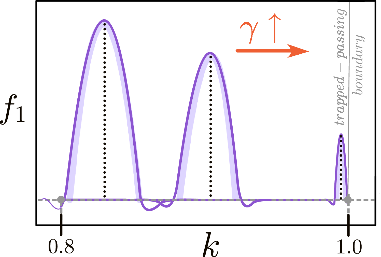
 q=m/n

 ν
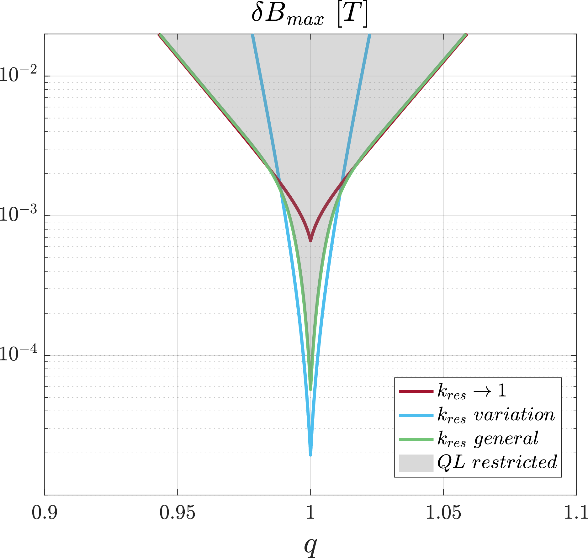
 δBmaxk→1
 δBmaxvar
 δBmaxgen

 Open access

