1. INTRODUCTION
In our modern society, the rapid advancements of technology have made computer systems easily available in diverse areas for various applications. A computer system basically consists of two parts: computer hardware and computer software. Although extensive research has focused on computer hardware reliability, the need and the importance for computer software quality are growing as the functionality of computer software becomes an essential and critical role. Furthermore, one of the most important attributes in software quality is software reliability, which has attracted an increasing amount of attention in the software engineering community. As a result, many models have been proposed to analyze software failure or reliability data (see, e.g., Musa, Iannino, and Okumoto [10], Singpurwalla and Wilson [17], and Pham [12]).
An important and practical application of software reliability is deciding when to stop testing and to release software; this application, which is specifically called the optimal software release problem, has been studied widely. Most of these software cost models are based on the nonhomogeneous Poisson process (NHPP). For example, Okumoto and Goel [11] proposed a cost-optimal software release policy to minimize the total expected software cost during the software development. Additionally, Yamada and Osaki [20] developed a cost–reliability-optimal software release policy. More examples can be found in Yamada, Narhisa, and Osaki [19], Kimura, Toyota, and Yamada [8], and Xie and Hong [18]. Meanwhile, Ross [14] considered a model with an estimating and stopping procedure. These approaches were followed by a Bayesian decision-theoretic approach suggested by Dalal and Mallows [6]. The work of Randolph and Sahinoglu [13] also provided a stopping rule based on a compound-Poisson model.
Additionally, Singpurwala and Soyer [15] contributed a nonhomogeneous autoregressive process, known as a Kalman filter, to describe reliability growth. Due to its superior predictive and tracking abilities for state space models (Singpurwalla and Wilson [16], Chen and Singpurwalla [5]), various Kalman filter models were discussed: to name a few, Gamma-Gamman-type invariant conditional distribution (Chen and Singpurwalla [4]) and exponential-Poisson-type invariant conditional distribution software reliability application (Chang and Leu [3]).
Cost is apparently a major factor during the process of software development; however, the reliability requirement is also an essential point, especially for the high-quality demanding systems such as the space shuttle. Following the discussion by Chang [2], our attention in this article focuses on the convergence of total testing time under the reliability constraint. In Section 2 we describe the cost model based on a non-Gaussian Kalman filter model. The convergence property of the total testing time with the reliability requirement is discussed in Section 3. We conclude by illustrating the framework with real data analysis.
2. MODELS
2.1. A Non-Gaussian Kalman Filter Model
Mainly because of their computational tractability, Gaussian Kalman filter models have been extensively used in many applications. However, the underlying distributions of failure data for software are generally highly skewed and, thus, the Gaussian assumption for modeling the data comes into question. Based on the idea of “invariant conditional distributions” introduced by Bather [1], Chen and Singpurwalla [4] developed a non-Gaussian Kalman filter model for tracking software failure data and this model outperformed the Gaussian model in its predictive performance. Consequently, this non-Gaussian Kalman filter model is used in our study.
A Kalman filter model is basically specified by two equations: an observation equation and a system equation. In the observation equation, we specify how observations and time change over different stages; however, the system equation describes how unknown parameters, θn and Cn, evolve with time. Let Tn represent the time between the (n − 1)st and the nth failure (nth stage), let θn represent the scale parameter of Tn, and let Dn = {T1,…,Tn} represent the collection of observations until n. Then the model is specified as follows:
Model Assumptions
The observation equation: (Tn|θn) ∼ Gamma(ωn,θn)
The system equation: (Cnθn /θn−1|θn−1) ∼ Beta(σn−1,υn−1)
The initial information: (θ0|D0) ∼ Gamma(σ0 + υ0,u0)
Cn, ωn,υn, and σn are assumed to be known and nonnegative. Furthermore, they are required to satisfy the condition

Results
The posterior of θn−1: (θn−1|Dn−1) ∼ Gamma(σn−1 + υn−1,un−1)
The prior of θn: (θn|Dn−1) ∼ Gamma(σn−1,Cnun−1)
The one-step forecast: (Tn /Cnun−1|Dn−1) ∼ Pearson type VI (p = ωn,q = σn−1); (see Johnson and Kotz [7, p.51])
The posterior for θn: (θn|Dn) ∼ Gamma(σn−1 + ωn,un), where un = Cnun−1 + Tn.
T0 ≥ 0 is arbitrarily chosen to reflect the best assessment about the interfailure time prior to observing any data. Given the history of the process, the conditional density of Tn is

According to Eq. (2.1), we can rewrite the one-step forecast as

Moreover, if ωn is a positive integer, then the reliability function in stage n is

2.2. A Cost Model
We define the following notations to present a cost model that specifies the cost of testing, of removing faults during the test phase, and of software failure during the mission time.

Additionally, we assume that (1) the cost for testing the system is proportional to the testing time, (2) the cost of removing each fault during the testing phase is a constant, and (3) the risk cost due to software failure is a constant. Accordingly, the expected software testing cost at the nth stage is

where Fn(t) = 1 − Rn(t) and Rn(x|t) = Rn(t + x)/Rn(t). The cost of removing a fault or bug during the testing phase should be much less than the cost of fixing it after release. Accordingly, we assume that c2 < c3.
2.3. The Algorithm and Properties of the Model
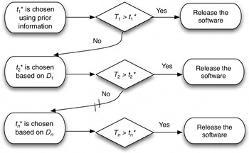
Without any reliability constraint, we can heuristically explain our model as a sequential software release algorithm. In the beginning, the optimal release time t1* is chosen according to prior information; that is, t1* is the root to minimize φ1(·). If the software's failure time is greater than the predetermined release time (i.e., T1 > t1*), then the software is released. Otherwise (i.e., T1 < t1*), we enter the next stage and the prior information for the second stage is updated. Simultaneously, an additional optimal release time t2* is chosen based on the updated information, T1. Let t2* be the value to minimize φ2(·). The software is released if T2 > t2*. Otherwise, the prior information is updated to the third stage, and the third optimal release time t3* is chosen, and so on. This proposed algorithm for determining the optimal release time does not minimize the expected total testing cost; however, it is designed to minimize the expected testing cost in every stage based on up-to-time information and assume that no more observation will be made in the future. Figure 1 is the flowchart showing our sequential steps.

Flowchart of the algorithm.
Note that in every stage, the optimal release time tn* minimizes the expected cost [Eq. (2.4)]. Thus, we have that

and it implies the finiteness of the optimal release time in every stage:

Specifically, the optimal release time in every stage can be determined by solving the following equation numerically:

Assume that n ≥ 0 and

. The remaining testing time after the nth stage is expressed as

if the software is actually released at stage m ≥ n + 1; in other words, Tm > tm* and Ti < ti* for all i < m.
For convenience, we do not allow the parameters to change from stage to stage but require them to have common fixed values. More specifically, we assume that σn ≡ σ > 1, Cn ≡ C ∈ (0,1), and ωn ≡ ω is a positive integer.
Lemma 1: If β ∼ Beta(ω,σ), then E [−ln(1 − β)] = −ln g(ω,σ), where

The proof of Lemma 1 is relegated to the Appendix.
In this article we restricted our cost model to the open loop–feedback optimal (OLFO) control problem; hence, we have the following theorem.
Theorem 1: Assume that our software reliability model satisfies Eqs. (2.1)–(2.3) and the cost model [Eq. (2.4)]. The total testing time Ttotal,0 and the total number of testing faults Ntotal,0 are finite when the following conditions are satisfied:
C > g(ω,σ).
The optimal release time, Tn*, is bounded in every stage (Tn* ≤ B, say).
Proof: According to Eq. (2.2), for all n ≥ 1, define

where βn ≡ Tn /(Tn + Cun−1) are independent and identical Beta(ω,σ) distributed. Equation (2.8) implies Cun = C × (Tn + Cun−1) = [C/(1 − βn)] × Cun−1, and we can iteratively repeat this process to obtain

.
According to condition (ii), the optimal release time is bounded in every stage. Therefore, the results will be proven if the failure time is greater than the optimal release time eventually under conditions. In other words, it is good enough to prove that Tn → ∞ almost surely as n → ∞. Here we will show that Eq. (2.9) holds under our conditions.

1. Provided C > g(ω,σ)(or C < g(ω,σ)),

2. For C = g(ω,σ), applying the central limit theorem, we have

where θ2 = Var([−ln(1 − β1)]). Thus, by Eq. (2.10),

From (1) and (2), we show Eq. (2.9) and it completes our proof of Theorem 1. █
3. RELEVANCE OF MODEL WITH RELIABILITY CONSTRAINT
Next, we discuss the optimal software release time with the software reliability requirement. It is also apparent to have a trade-off between releasing and keep testing. If we save the cost for testing and release too early, the cost might significantly increase due to the bug-fixing requests from customers. However, if we just keep testing in order to get bug-free systems, the cost for testing might be significant and also the software's place in the market might be lost. Thus, it is important to find a balance point. However, the requirement of reliability might differ enormously for different software systems. In actuality, some systems might require extremely high reliability, such as a military defense system, but others might not. Therefore, the reliability constraint should be incorporated in our release policy.
In this section we will treat both the software testing cost [Eq. (2.4)] and the reliability rate Rn(x|t) ≡ Rn(t + x)/Rn(t) as the evaluation criteria. In addition to minimize the expected software testing cost, the optimal release time is also constrained to attain a desired reliability level R0. Thus, the optimal software release problem is formulated as follows:

Note that

Using Eq. (2.1), if ωn > 1, we have ∂Rn(x|t)/∂t → −fn(x) as t → 0. Thus, Rn(x|t) is decreasing in t on the neighborhood of zero. We rewrite Eq. (2.3) as

Hence, the conditional reliability is

or

Since Rn(x|t) is a continuous function of t, there exists at least one value of t (say tR) such that Rn(x|t) ≥ R0 for all t ≥ tR. Let tR,n be the minimum value of tR such that Rn(x|t) ≥ R0, namely tR,n = min{tR ≥ 0|Rn(x|t) ≥ R0, ∀t ≥ tR}. From the above discussion, we know tR,n exists in every stage. Then it is reasonable to reformulate our problem as

hence, the optimal release time tR,n* = arg mint≥tR,n φn(t) also exists in every stage.
Next, we will prove the total testing time is finite with probability 1 under the reliability constraint. Using Eq. (3.2), we have

Thus, Rn(x|t) ≥ R0 if

or

This implies

Now from the definition of tR,n*, we have, for all n ≥ 1,

and it implies

In other words, the conditions of Theorem 1 hold for our case and, as a result, we have that both the total testing time Ttotal,0 and the total number of testing faults Ntotal,0 are finite.
4. NUMERICAL EXAMPLE
We illustrate the framework of our model by using an existing dataset; this popular dataset was collected by Musa [9] on 16 software systems to assist in monitoring the status and predicting schedules. Among them, the first 4 systems of the 16 were collected with the author being the responsible manager; the remaining 12 were collected with the guidance of the author. In order to illustrate the workings of our cost model, “system 1” is selected in our study.
Set σn = 2, ωn = υn = 1, and Cn = C = 0.64 and the model satisfies the assumptions in Theorem 1. According to Eq. (2.1), the conditional density of Tn given the history of the process is

and its distribution function is
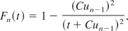
According to Eq. (4.2),

or we know Rn(x|t) ≥ R0 when t ≥ R01/2x/(1 − R01/2) − Cun−1.
From a previous discussion, we know the optimal release time for every stage can be obtained by solving Eq. (2.6); namely the optimal release time for every stage is the root of the equation

To attain the predetermined reliability requirement, we set tR,n = R01/2x/(1 − R01/2) − Cun−1.
As we discussed in Section 2, the risk cost due to software failure is naturally much higher than the testing cost. Otherwise, software testing is not necessary and does not make any sense. Therefore, we set up the cost of coefficients c1 = 0.1, c2 = 1, c3 = 5000, and the mission time x = 800 for our case to study.
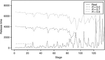
To illustrate the framework of our model, we study the cases with different reliability requirement levels, R0 = 0.7 and R0 = 0.8. Additionally, the unconstraint case, R0 = 0.0, is included in our study to compare the impact of the reliability requirement on the software release time.
The time to detect faults and the optimal release time in every stage are depicted in Figure 2. The solid line represents the true time to detect faults in Musa's “system 1.” The optimal release times based on the current stage's process history are shown in a dot-dash, dashed, and dotted lines according to its reliability requirement after the first stage. Once the optimal release time is less than the failure time, the software will be released. Otherwise, the testing will enter the next stage. Apparently, the higher the reliability requirement, the longer the optimal release time in every stage. From Figure 1, we notice that the software is released at stages 28, 93, and 129, respectively. In other words, software will take longer to test for releasing while meeting the reliability requirement and the constraint increases. This finite stopping time also validates our theorem.

Comparison of release time with different reliability requirements.
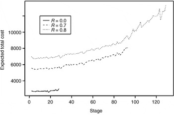
Another concern for software development is cost. Figure 3 gives the expected total cost in every stage. Provided that n + K is the last testing stage, the expected total cost in stage n is defined as follows:


Comparison of expected total cost in every stage.
where K ≥ 1. It is apparent that increasing the value of R0 will result in a greater testing cost. Note that the optimal release time tn* does not minimize the expected total test cost; it just minimizes the expected test cost in every stage under the assumption that no more data will be observed in the future. Thus, the expected total cost in an earlier stage might be higher than the cost in a latter stage. However, the expected total testing cost is still an increasing trend.
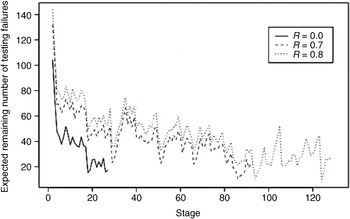
Finally, in Figure 4 we display the expected remaining number of testing faults after the nth stage. From Figure 4 we can see a decreasing trend for the remaining number of testing failures although it is not really decreasing for each stage. This can be partly explained by an imperfectly debugging property of testing, which is also an interesting and practical problem in the software development community.

Expected remaining number of testing failures after the nth stage.
Acknowledgment
The research by Y.C. Chang was supported by the National Science Council of ROC grant NSC 93-2118-M-238-002.
Appendix: Proof of Lemma 1
From the assumption that β ∼ Beta(ω,σ), the density function of β is

Let Y = −ln(1 − β); we then have β = 1 − exp(−Y) and dβ = exp(−Y) dY.
Case 1: ω ≠ 1 and σ ≠ 1. The density of Y can be expressed as

Therefore,

Case 2: ω = 1 and σ = 1. Under this case, β reduces to the uniform (0, 1) and the transformed variable Y = −ln(1 − β) will follow an exponential distribution with mean one, which can be expressed as Eq. (A1).
Case 3: ω = 1 and σ ≠ 1.
Case 4: ω ≠ 1 and σ = 1.
In Cases 3 and 4, the density functions of β are strictly decreasing and strictly increasing, respectively. The proofs are omitted since they are similar to the proof of Case 1. █