2.1 Basic equations

The starting point of this study is the continuity and momentum equations in a compressible fluid without any gravity effects:

where $\unicode[STIX]{x1D70C}$ , $\boldsymbol{v}$ , $p$ , $\unicode[STIX]{x1D707}$ and $\unicode[STIX]{x1D701}$ are the density, velocity, pressure, first coefficient of viscosity and second coefficient of viscosity (under the Stokes assumption, $\unicode[STIX]{x1D701}=-(2/3)\unicode[STIX]{x1D707}$ ) respectively. We now divide the density, velocity and pressure fields into mean and fluctuating components, i.e. $v_{i}=U_{i}+u_{i}$ , $\unicode[STIX]{x1D70C}=\overline{\unicode[STIX]{x1D70C}}+\unicode[STIX]{x1D70C}^{\prime }$ and $p=\overline{p}+p^{\prime }$ , where $U_{i}$ , $\overline{\unicode[STIX]{x1D70C}}$ and $\overline{p}$ are the mean components and $u_{i}$ , $\unicode[STIX]{x1D70C}^{\prime }$ and $p^{\prime }$ are the fluctuating components. In the Reynolds averaged equation, we assume $\unicode[STIX]{x1D70C}^{\prime }\ll \overline{\unicode[STIX]{x1D70C}}$ and neglect $\unicode[STIX]{x1D70C}^{\prime }$ when $\overline{\unicode[STIX]{x1D70C}}$ exists, and the density is linearized. This preserves the triad resonant condition in Fourier space, as seen in incompressible turbulence (Marion, Bertoglio & Mathieu Reference Marion, Bertoglio and Mathieu1988).

2.2 Rapid distortion theory assumptions for the turbulence–shock-wave interaction

Rapid distortion theory is a method for solving linearized governing equations under rapid deformation using a statistical technique; RDT solutions are exact solutions of the Navier–Stokes equations if the initial flow is a single plane wave, because the nonlinear terms are exactly zero throughout the triad interaction (Craik & Criminale Reference Craik and Criminale1986; Kevlahan & Hunt Reference Kevlahan and Hunt1997). Rapid distortion theory equations are obtained by neglecting the nonlinear terms in (2.18) and (2.19) which linearize the equations; this allows analytical solutions for a number of cases. The details of RDT can be found in Hunt & Carruthers (Reference Hunt and Carruthers1990), Hunt & Kevlahan (Reference Hunt and Kevlahan1993) and Kevlahan & Hunt (Reference Kevlahan and Hunt1997).

Figure 1.

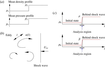
(a) Mean density and pressure profiles via the Rankine–Hugoniot relation, where the subscript 1 denotes the front of the planar shock wave and the subscript 2 denotes the back of the planar shock wave. (b) Schematic of the interaction between turbulence and a shock wave. (c) Schematic of the RDT analysis region.

Figure 1 shows a schematic of the turbulence–shock-wave interaction. The time scale of the turbulence–shock-wave interaction, $T_{SW}$ , is found to be small relative to the turbulence characteristic time scale, $\unicode[STIX]{x1D70F}(l)\sim l/u(l)$ , where $l$ is the turbulence characteristic length scale and $u(l)$ is a turbulence characteristic velocity. In addition, if the linear effects of the compression (e.g.  ${\sim}|S_{1}|(u(l)/l)$ for a compressing distortion) on the vorticity $\unicode[STIX]{x1D74E}$ are much stronger than the nonlinear self-induced compression by the turbulence ( ${\sim}(u(l)/l)^{2}$ ), the nonlinear terms do not play an important role. When turbulence is compressed by a planar shock wave, the strength of the characteristic compression can be given by

where $\unicode[STIX]{x1D6FF}_{SW}$ is the thickness of the region influenced by the shock-induced compression, $U_{SW}$ is the speed of the shock wave and $u_{0}$ is the mean velocity in front of the shock. Thus, the following relations are assumed for the interaction between turbulence and a shock wave:

Equation (2.22a ) is valid for small values of $T_{SW}$ , whereas (2.22b ) is valid for large values of $|S_{1}|$ . An overall criterion for the validity of RDT for calculating the statistics of the energy-containing eddies in a given turbulent flow can be derived from (2.22) in terms of the r.m.s. velocity $u_{0}$ and the integral length scale $L$ (Kevlahan & Hunt Reference Kevlahan and Hunt1997). This leads to

where $T_{L}$ is the integral time scale. This can be re-expressed as

This criterion should be valid at the start of the distortion. In the present RDT analysis, the deformation of the shock wave is ignored. Kevlahan (Reference Kevlahan1997) showed that the vorticity jump is connected with the shock curvature, the baroclinic effect and the conservation of angular momentum. In RDT analysis, vorticity amplification is interpreted as being caused by the angular momentum created by compression of the flow in the direction normal to the shock wavefront. Therefore, one must note that the present analysis is limited to the case in which the deformation of the shock wave can be ignored. Based on DNS results (Lee et al. Reference Lee, Lele and Moin1993; Larsson et al. Reference Larsson, Bermejo-Moreno and Lele2013), the deformation of a shock wave is slight for $M_{t}/(M_{s}-1)\ll 1$ , and therefore RDT is valid for $M_{t}/(M_{s}-1)\ll 1$ . The bases of the inviscid RDT equations are (2.13),

It should be noted that the dilatational mode in (2.26) disappears because of the symmetrical form of $S_{lj}(t)=\unicode[STIX]{x1D6FF}_{l1}S_{11}(t)\unicode[STIX]{x1D6FF}_{j1}$ . For one-dimensional compression, (2.26) is the same as in Mahesh et al. (Reference Mahesh, Lele and Moin1994) without shear. However, these authors did not obtain the analytical solutions and only performed a numerical analysis. The solutions to the system are expected to have the form

where $\boldsymbol{G}$ are Green functions.

2.3 Ordinary differential equations and analytical solution for inviscid RDT

We consider the analytical solution of the inviscid RDT equations. From (2.26) and the solenoidal condition (2.17), we obtain

Here, the method for solving the ordinary differential equations (ODEs) is described briefly, because cumbersome calculations are required to solve them analytically (see appendix A for details). The ODE will be set to $(\text{d}\hat{u} _{i}^{s}(\unicode[STIX]{x1D74C},t))/\text{d}t=A_{ij}(t)\hat{u} _{j}^{s}(\unicode[STIX]{x1D74C},t)$ if the tensor notation of (2.29) is utilized. We then determine the eigenvalues of $A_{ij}(t)$ . After some algebra, the eigenvalues of $A_{ij}(t)$ are as follows:

Each eigenvector can be obtained for the acquired eigenvalues. Let $\unicode[STIX]{x1D609}_{ij}$ be the transformation matrix which consists of eigenvectors. A diagonal matrix $\unicode[STIX]{x1D60B}_{\unicode[STIX]{x1D6FC}\unicode[STIX]{x1D6FD}}(t)$ can be expressed as $\unicode[STIX]{x1D60B}_{\unicode[STIX]{x1D6FC}\unicode[STIX]{x1D6FD}}(t)=\unicode[STIX]{x1D609}_{\unicode[STIX]{x1D6FC}i}^{-1}A_{ij}(t)\unicode[STIX]{x1D609}_{j\unicode[STIX]{x1D6FD}}$ . Multiplying $\unicode[STIX]{x1D609}_{ij}^{-1}$ to (2.29) from the left side, we obtain $(\text{d}y_{i}(\unicode[STIX]{x1D74C},t))/\text{d}t=\unicode[STIX]{x1D60B}_{ij}(t)y_{j}(\unicode[STIX]{x1D74C},t)$ , where $y_{i}(\unicode[STIX]{x1D74C},t)=\unicode[STIX]{x1D609}_{ij}^{-1}\hat{u} _{i}^{s}(\unicode[STIX]{x1D74C},t)$ . Because $\unicode[STIX]{x1D60B}_{ij}(t)$ is a symmetrical tensor, which has only diagonal components, the solution to $y_{i}(\unicode[STIX]{x1D74C},t)$ is obtained using separation of variables. If the relationship $\hat{u} _{i}^{s}(\unicode[STIX]{x1D74C},t)=\unicode[STIX]{x1D609}_{ij}y_{j}(\unicode[STIX]{x1D74C},t)$ and the initial conditions $y_{i}(\boldsymbol{k},0)=\unicode[STIX]{x1D609}_{ij}\hat{u} _{j}^{s}(\boldsymbol{k},0)$ are used, analytical solutions are given by

where

For convenience in later discussions, the analytical solutions in the Craya–Herring decomposition are given by

Interestingly, the vortex mode, $\hat{u} ^{(1)}(\unicode[STIX]{x1D74C},t)$ , is not affected by the rapid one-dimensional compression, whereas the wave mode, $\hat{u} ^{(2)}(\unicode[STIX]{x1D74C},t)$ , is strongly affected. Thus, the vorticity in the one-dimensional compressed direction does not change throughout the turbulence–shock-wave interaction in the limiting case, as discussed later. This situation is similar to that in stratified turbulence (Hanazaki & Hunt Reference Hanazaki and Hunt1996). The fact that the vorticity does not change in the compressed direction is a direct result of the jump conditions for vorticity. Kevlahan (Reference Kevlahan1997) also showed that the vorticity only increases in the plane tangent to a shock wave.

After some algebra, the inviscid RDT equation for the dilatational mode becomes

where $R(t)$ is given by

and the left-hand side of (2.38) is a typical Sturm–Liouville equation. Thus, the analytical solution is assumed to be a special function such as a Legendre function (e.g. Hanazaki & Hunt Reference Hanazaki and Hunt2004). In general, the analytical solution will take the form $\hat{u} ^{d}(\unicode[STIX]{x1D74C},t)=u_{0}(t)+C_{1}u_{1}(t)+C_{1}u_{2}(t)$ , where $u_{0}$ is a particular solution, and $u_{1}(t)$ and $u_{2}(t)$ are basis solutions. If one basis solution is found, the analytical solution of the dilatational mode can be obtained. When $S_{1}=0$ , the analytical solutions are expressed by trigonometric functions (Marion et al. Reference Marion, Bertoglio and Mathieu1988). Unfortunately, we could not find any analytical solutions for the dilatational mode. Thus, hereinafter we only discuss the RDT solutions of the solenoidal mode. It should be noted that Jacquin et al. (Reference Jacquin, Cambon and Blin1993) found the analytical solution for the case in which the second term of (2.38) is neglected.

4.1 Model spectra for homogeneous isotropic turbulence (model spectrum A)

The following model spectrum describes the different forms of energy over a wide range of wavenumbers (Davidson Reference Davidson2004):

where $K_{0}$ corresponds to the Kolmogorov constant, which was set to 1.52 in this study, and $m$ corresponds to the parameter that determines the slope of the energy spectrum at low wavenumbers: $E(k\rightarrow 0)\sim k^{2}$ for $m=11/2$ and $E(k\rightarrow 0)\sim k^{4}$ for $m=17/2$ . In this study, we adopted a Saffman-type energy spectrum as an initial condition because there is experimental evidence of Saffman turbulence in grid turbulence (Krogstad & Davidson Reference Krogstad and Davidson2010; Kitamura et al. Reference Kitamura, Nagata, Sakai, Sasoh, Terashima, Saito and Harasaki2014). In this study, the model spectrum (4.1) was transformed as a function of $Re_{\unicode[STIX]{x1D706}}$ to investigate the dependence on turbulence of the Reynolds number based on the Taylor microscale for the non-zero-viscosity RDT solutions. Using Taylor–Kolmogorov scaling, $\unicode[STIX]{x1D702}/L\approx 15^{3/4}Re_{\unicode[STIX]{x1D706}}^{-3/2}$ , the transformed model spectrum is described by

In this study, we investigated the following $Re_{\unicode[STIX]{x1D706}}$ dependences for non-zero-viscosity RDT: (i)  $Re_{\unicode[STIX]{x1D706}}=10^{2}$ and (ii)  $Re_{\unicode[STIX]{x1D706}}=10^{4}$ . The turbulent flow at $Re_{\unicode[STIX]{x1D706}}=10^{2}$ is a typical flow such as grid turbulence, whereas the turbulent flow at $Re_{\unicode[STIX]{x1D706}}=10^{4}$ is a typical flow such as atmospheric turbulence.

4.2 Model spectra for homogeneous axisymmetric turbulence

Sreenivasan & Narasimha (Reference Sreenivasan and Narasimha1978) proposed that a homogeneous axisymmetrical tensor can be described by the expansion in zonal harmonics of the two independent scalar functions. The terms $A_{1}$ and $A_{2}$ can be expanded in zonal harmonics with the Legendre polynomial $P_{2m}(\cos \unicode[STIX]{x1D703})$ as a basis function:

The expansion in terms of spherical harmonics was generalized by Cambon & Teissèdre (Reference Cambon and Teissèdre1985) for arbitrary anisotropy. This expansion is consistent with that of Sreenivasan & Narasimha (Reference Sreenivasan and Narasimha1978) for axisymmetry.

By postulating that some pair of functions $A_{i}$ $(i=1,\ldots ,4)$ depends only on $k$ and not on $\cos \unicode[STIX]{x1D703}$ , and using (4.3) and (4.4), a more concrete form of the energy spectral tensor can be obtained. Sreenivasan & Narasimha (Reference Sreenivasan and Narasimha1978) proposed the following three ansatzes for homogeneous axisymmetric turbulence.

1. (i) Ansatz 1: $A_{1}$ and $A_{2}$ depend only on $k$ .

2. (ii) Ansatz 2: $A_{2}$ and $A_{3}$ depend only on $k$ .

3. (iii) Ansatz 3: $A_{1}$ and $A_{3}$ depend only on $k$ .

In these three ansatzes, Ansatz 1 is the simplest model because the angular dependence appears throughout $P_{ij}(\boldsymbol{k})$ and $H_{ij}(\boldsymbol{k})$ . Ansatz 2 is the more harmonic form (as compared with Ansatz 1) because it contains higher-order Legendre polynomials, e.g. $F_{2}(k)P_{2}(\cos \unicode[STIX]{x1D703})$ . In Ansatz 3, $A_{2}(k,\cos \unicode[STIX]{x1D703})$ can be expressed as $A_{2}(k,\cos \unicode[STIX]{x1D703})=(1/\cos ^{2}\unicode[STIX]{x1D703})[A_{3}-k^{2}A_{1}]$ , where $A_{3}$ and $A_{1}$ are functions of $k$ . As mentioned by Sreenivasan & Narasimha (Reference Sreenivasan and Narasimha1978), $A_{1}(k,\cos \unicode[STIX]{x1D703})$ and $A_{2}(k,\cos \unicode[STIX]{x1D703})$ do not depend on the angular dependence when $k^{2}A_{1}=-A_{3}$ ; therefore, they become isotropic forms. On the other hand, $A_{2}(k,\cos \unicode[STIX]{x1D703})$ exhibits singularity for $\cos \unicode[STIX]{x1D703}=0$ when $k^{2}A_{1}\neq -A_{3}$ .

From the abovementioned background for the three ansatzes, we used Ansatzes 1 and 2 for the model spectra.

5.1 Angular distribution of the energy spectral tensor

In homogeneous anisotropic turbulence, there is an angular dependence for $Q^{(1)}(\unicode[STIX]{x1D74C},t)$ and $Q^{(2)}(\unicode[STIX]{x1D74C},t)$ . When we discuss the departure from isotropy, it is convenient to introduce the $e$ – $z$ decomposition (Sagaut & Cambon Reference Sagaut and Cambon2008). For instance, the angular dependence of the anisotropic turbulence has been discussed by Cambon, Mansour & Godefeferd (Reference Cambon, Mansour and Godefeferd1997). However, in this study, the angular distribution of the parallel and perpendicular energy spectral tensors is discussed to better understand the phenomena in turbulence–shock-wave interactions.

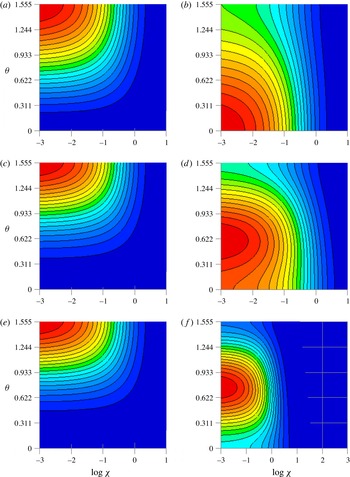
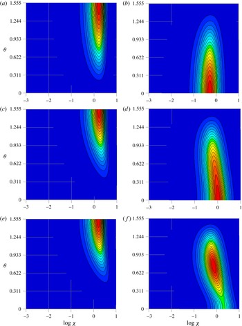
Figures 2 and 3 show the changes in angular dependence of the energy spectral tensors, $\unicode[STIX]{x1D6F7}_{\Vert }(\unicode[STIX]{x1D74C},t)$ and $\unicode[STIX]{x1D6F7}_{\bot }(\unicode[STIX]{x1D74C},t)$ , for model spectra A and B respectively. In model spectrum A, the spectral tensor has energy at low wavenumbers, and this is caused by the Saffman form at low wavenumbers, whereas in model spectrum B (and C, not shown), the spectral tensor has energy near the inverse of the integral length scale, and this is due to the Batchelor form at low wavenumbers. When initial isotropic conditions are considered, there is a slight change in the angular distribution of $\unicode[STIX]{x1D6F7}_{\Vert }(\unicode[STIX]{x1D74C},t)$ , whereas the energy concentrates to approximately $\unicode[STIX]{x1D703}=\unicode[STIX]{x03C0}/4$ in the angular distribution of $\unicode[STIX]{x1D6F7}_{\bot }(\unicode[STIX]{x1D74C},t)$ . As shown in figures 2 and 3, the shock-induced one-dimensional compression (hereinafter simply ‘compression’) transfers energy to high wavenumbers. This energy transfer was seen in $\unicode[STIX]{x1D6F7}_{\bot }(\unicode[STIX]{x1D74C},t)$ , regardless of the choice of Ansatz 1 or 2. On the other hand, there was a slight difference in $\unicode[STIX]{x1D6F7}_{\Vert }(\unicode[STIX]{x1D74C},t)$ between Ansatzes 1 and 2. These different changes contribute to the changes in the one-dimensional spectra at low wavenumbers. As discussed later, the energy changes at $\unicode[STIX]{x03C0}/2$ in $\unicode[STIX]{x1D6F7}_{\bot }(\unicode[STIX]{x1D74C},t)$ yield large changes at low wavenumbers in the compressed direction, whereas there are no changes in the longitudinal one-dimensional spectra at low wavenumbers because the energy remains at $\unicode[STIX]{x03C0}/2$ in $\unicode[STIX]{x1D6F7}_{\Vert }(\unicode[STIX]{x1D74C},t)$ .

Figure 2.

The angular distribution of the energy spectral tensors in homogeneous isotropic turbulence for model spectrum A (the Saffman–Pao model spectrum, $Re_{\unicode[STIX]{x1D706}}=10^{2}$ ) as an initial condition ( $\log \unicode[STIX]{x1D712}$ – $\unicode[STIX]{x1D703}$ plot). (a,c,e) The angular distribution of $\unicode[STIX]{x1D6F7}_{\Vert }(\unicode[STIX]{x1D74C},t)$ . (b,d,f) The angular distribution of $\unicode[STIX]{x1D6F7}_{\bot }(\unicode[STIX]{x1D74C},t)$ . Panels (a,b), (c,d) and (e,f) correspond to $\overline{\unicode[STIX]{x1D70C}}/\unicode[STIX]{x1D70C}_{0}=1$ , $\overline{\unicode[STIX]{x1D70C}}/\unicode[STIX]{x1D70C}_{0}=2$ and $\overline{\unicode[STIX]{x1D70C}}/\unicode[STIX]{x1D70C}_{0}=4$ respectively. It should be noted that each colour contour is normalized by the maximum value in each figure.

Figure 3.

The same data as figure 2 but for model spectrum B with exponential form and $R_{u}=7/4$ .

As shown in figures 2 and 3, the changes in the energy spectral tensors strongly depend on the initial distributions of the energy spectral tensors. Thus, we can interpret the change in the angular distribution as the effect of the initial anisotropy. When the initial anisotropy is strong, as discussed later, the amplifications of velocity variances are larger than in the case of homogeneous isotropic turbulence. These results suggest that the change in turbulence after compression is different for the near and far regions of the grid turbulence. In fact, these differences have been reported by Agui et al. (Reference Agui, Briassulis and Andreopoulos2005). Regardless of the initial energy spectral tensors, the distribution of $\unicode[STIX]{x1D6F7}_{\Vert }(\unicode[STIX]{x1D74C},t)$ tends to concentrate at $\unicode[STIX]{x1D703}=\unicode[STIX]{x03C0}/2$ , whereas that of $\unicode[STIX]{x1D6F7}_{\bot }(\unicode[STIX]{x1D74C},t)$ tends to concentrate at $\unicode[STIX]{x1D703}=\unicode[STIX]{x03C0}/4$ .

5.2 Velocity variances

When isotropic initial conditions are considered, $Q^{(1)}(k)=Q^{(2)}(k)=E(k)/4\unicode[STIX]{x03C0}k^{2}$ . From (3.6), (3.9) and (3.10), the energy spectral tensors are given by

where

is the initial TKE of the solenoidal mode. The variances of the parallel and perpendicular velocity fluctuations are given by

and the TKE of the solenoidal mode is given by

where $C=\overline{\unicode[STIX]{x1D70C}}/\unicode[STIX]{x1D70C}_{0}$ . The limiting cases for (5.5) and (5.6) have been derived by Ribner & Tucker (Reference Ribner and Tucker1953). For Ansatzes 1 and 2, the changes in each velocity variance and TKE value are described in § C.1. As confirmed by Larsson & Lele (Reference Larsson and Lele2009) using DNS, the maximum wavenumber, which corresponds to the resolution in the physical space, is important in turbulence–shock-wave interactions. Using RDT analysis, Jacquin et al. (Reference Jacquin, Cambon and Blin1993) obtained the TKE after the compression using the integration range $[k_{0,min}:k_{0,max}]$ for the initial homogeneous isotropic turbulence. However, as shown in the experiment of Barre et al. (Reference Barre, Alem and Bonnet1996), the TKE at high wavenumbers increases behind a shock wave. Furthermore, Larsson & Lele (Reference Larsson and Lele2009) showed that different numerical resolutions yielded different amplification ratios of velocity variance, and that their DNS results were different from those of Lee et al. (Reference Lee, Lele and Moin1997) and the LIA. Therefore, the maximum wavenumber, which corresponds to the resolution in the physical space, plays an important role in the statistical quantities of turbulence. In homogeneous turbulence, the TKE dissipation of the solenoidal mode is expressed by $\unicode[STIX]{x1D716}^{s}=\unicode[STIX]{x1D708}\langle \unicode[STIX]{x1D74E}^{2}\rangle$ . Thus, the Kolmogorov length scale is expressed by $\unicode[STIX]{x1D702}=(\unicode[STIX]{x1D708}^{2}/\langle \unicode[STIX]{x1D74E}^{2}\rangle )^{1/4}=(\overline{\unicode[STIX]{x1D707}}^{2}/\overline{\unicode[STIX]{x1D70C}}^{2}\langle \unicode[STIX]{x1D74E}^{2}\rangle )^{1/4}$ , and the ratio between the Kolmogorov length scales after and before the interaction with a shock wave can be written as follows using $\sqrt{\langle \unicode[STIX]{x1D74E}^{2}\rangle }/\sqrt{\langle \unicode[STIX]{x1D74E}_{0}^{2}\rangle }\sim \overline{\unicode[STIX]{x1D70C}}/\unicode[STIX]{x1D70C}_{0}$ (Mahesh et al. Reference Mahesh, Lele and Moin1997):

where $(\overline{\unicode[STIX]{x1D707}}/\unicode[STIX]{x1D707}_{0})^{2}=f(\overline{T})$ indicates that $\overline{\unicode[STIX]{x1D707}}$ is an increasing function of temperature $\overline{T}$ . Larsson & Lele (Reference Larsson and Lele2009) proposed a maximum wavenumber of $k_{max}/k_{0,max}=(\overline{\unicode[STIX]{x1D70C}}/\unicode[STIX]{x1D70C}_{0})(T_{0}/\overline{T})^{3/8}$ . 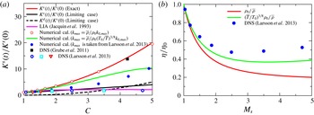Here, we adopted a maximum wavenumber of $k_{max}>(\overline{\unicode[STIX]{x1D70C}}/\unicode[STIX]{x1D70C}_{0})k_{0,max}$ in the numerical calculation. Figure 4(a,b) shows the changes in the TKE and the changes in $\unicode[STIX]{x1D702}/\unicode[STIX]{x1D702}_{0}(=\,k_{0,max}/k_{max})$ . When we set the maximum wavenumber to $k_{max}>(\overline{\unicode[STIX]{x1D70C}}/\unicode[STIX]{x1D70C}_{0})k_{0,max}$ , the obtained results agreed with the exact solution (5.7). 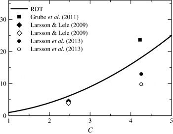On the other hand, when we set the maximum wavenumber to $k_{max}/k_{0,max}=(\overline{\unicode[STIX]{x1D70C}}/\unicode[STIX]{x1D70C}_{0})(T_{0}/\overline{T})^{3/8}$ as used in Larsson & Lele (Reference Larsson and Lele2009) and Larsson et al. (Reference Larsson, Bermejo-Moreno and Lele2013), the TKE amplification was underestimated in the RDT analysis. As confirmed by the high-resolution DNS of Larsson & Lele (Reference Larsson and Lele2009), the obtained results depend on the resolution. Furthermore, our RDT results suggest that the dependence on the resolution for the statistical quantities becomes remarkable with increase of Mach number. Thus, RDT analysis strongly suggests that high-resolution DNS is needed to obtain accurate results for turbulence–shock-wave interactions, especially for high-Mach-number flows. Of course, RDT is based on a linear theory, and the requirements of grid resolution for high-Mach-number flows should be carefully examined using DNS in future studies. The TKE amplification of the DNS results of Grube et al. (Reference Grube, Taylor and Martin2011) is shown in figure 4; their results are in good agreement with the RDT analysis. The LIA result in the near field (Jacquin et al. Reference Jacquin, Cambon and Blin1993) is also included in figure 4. Based on this result, $k_{max}>(\overline{\unicode[STIX]{x1D70C}}/\unicode[STIX]{x1D70C}_{0})k_{0,max}$ is used for the RDT analysis with non-zero viscosity in § 6.

Figure 4.

The amplification of the TKE versus the inviscid RDT solution for the initial homogeneous isotropic turbulence. Also included are the changes in the TKE from the LIA (near-field) result of Jacquin et al. (Reference Jacquin, Cambon and Blin1993) and the DNS result of Grube et al. (Reference Grube, Taylor and Martin2011) with the initial conditions $Re_{\unicode[STIX]{x1D706}}=26$ , $M_{t}=0.52$ and $M_{1}=3.46$ , and Larsson et al. (Reference Larsson, Bermejo-Moreno and Lele2013) with the initial condition $Re_{\unicode[STIX]{x1D706}}\approx 40$ , where $M_{1}$ is the Mach number of the upstream of a shock wave.

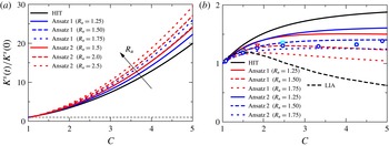
Figure 5(a) shows the amplification of the TKE for initial homogeneous axisymmetric turbulence. The amplification of the TKE depends on the initial degree of anisotropy; however, there is almost no dependence on the difference between Ansatzes 1 and 2. As discussed later, the amplification of $\langle u_{\bot }^{2}(t)\rangle$ contributes to the amplification of the TKE for the initial homogeneous axisymmetric turbulence. Figure 5(b) shows the changes in velocity anisotropy $\langle u_{\Vert }^{2}(t)\rangle /\langle u_{\Vert }^{2}(0)\rangle /(\langle u_{\bot }^{2}(t)\rangle /\langle u_{\bot }^{2}(0)\rangle )$ . The results of Larsson et al. (Reference Larsson, Bermejo-Moreno and Lele2013) for the far region are also included for reference. The changes in anisotropy against $\overline{\unicode[STIX]{x1D70C}}/\unicode[STIX]{x1D70C}_{0}$ for RDT are closer to the DNS results rather than the LIA result. Here, it is worth mentioning the difference between RDT and the LIA. First, the changes in the TKE in the near regions are associated with the energy transfer from the acoustic potential energy in the LIA. However, such changes are not incorporated into RDT. Thus, the predictive capabilities of the RDT analysis for turbulence–shock interaction are limited to only the vicinity of the shock wave. In the vicinity of the shock wave, the RDT result qualitatively agrees with the DNS result (Larsson & Lele Reference Larsson and Lele2009) in that the parallel component of the velocity fluctuations is amplified more than the perpendicular component. However, the LIA result shows the opposite result for $M_{s}=2.0$ (Lee et al. Reference Lee, Lele and Moin1997). This means that RDT is more accurate in the vicinity of the shock wave, whereas it cannot predict the statistical quantities for the far field. Then, RDT does not take into account of the entropy fluctuations. It is known that the entropy fluctuations are more significant than the acoustic fluctuations for high-Mach-number flows. Thus, the present RDT analysis is no longer valid for an inflow having the entropy fluctuations.

Figure 5.

(a) The amplification of the TKE versus the inviscid RDT solution for initial homogeneous axisymmetric turbulence. (b) The changes in $\langle u_{\Vert }^{2}(t)\rangle /\langle u_{\Vert }^{2}(0)\rangle /(\langle u_{\bot }^{2}(t)\rangle /\langle u_{\bot }^{2}(0)\rangle )$ . The symbols are taken from the DNS of Larsson et al. (Reference Larsson, Bermejo-Moreno and Lele2013); their results correspond to the post-shock turbulence anisotropy in the far field.

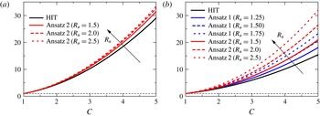
Figure 6 shows the changes in $\langle u_{\Vert }^{2}(t)\rangle$ and $\langle u_{\bot }^{2}(t)\rangle$ . As shown in figure 6, the changes in the variance of each velocity component depend on the initial degree of anisotropy. For the changes in $\langle u_{\bot }^{2}(t)\rangle$ , Ansatzes 1 and 2 yield different amplifications. When isotropic initial conditions are considered, the anisotropy of the velocity components is significant, but the anisotropy of the velocity components is not significant when the initial anisotropy is strong. However, this strong anisotropy cannot be seen in fully developed grid turbulence, as already shown in figure 5(b). Thus, the anisotropy of the velocity components may be a general consequence of homogeneous isotropic turbulence–shock-wave interactions.

Figure 6.

The amplification of velocity variances versus the inviscid RDT solution. (a) The variance of the parallel velocity components, $\langle u_{\Vert }^{2}(t)\rangle /\langle u_{\Vert }^{2}(0)\rangle$ , and (b) the variance of the perpendicular velocity components, $\langle u_{\bot }^{2}(t)\rangle /\langle u_{\bot }^{2}(0)\rangle$ . It should be noted that the changes in variance of the parallel velocity components for Ansatz 1 are the same as those for initial homogeneous isotropic turbulence, regardless of the initial anisotropy.

As shown in the DNS of Grube et al. (Reference Grube, Taylor and Martin2011), there is a slight contribution from the nonlinear term in the energy budget; however, it should be noted that the compressible contribution is much larger than the nonlinear effect. In addition, there is a slight contribution from the baroclinic effect. Following Kevlahan & Hunt (Reference Kevlahan and Hunt1997), we simply evaluate the evolution of the nonlinear term of the solenoidal mode by means of the primitive perturbation method. By non-dimensionalizing the equations for $\hat{u} _{i}^{s}(\unicode[STIX]{x1D74C},t)$ and $\unicode[STIX]{x1D74C}$ by the initial integral scale and the initial r.m.s. velocity $u_{0}$ , (2.19) and (2.20) become

where $\unicode[STIX]{x1D6FF}=(u_{0}/L)/|S_{1}|\ll 1$ is the ratio of the strain rate of the energy-containing eddies to the strength of compression and $Re_{L}=u_{0}L/\unicode[STIX]{x1D708}$ is the Reynolds number; $N_{i}^{s}(\hat{\boldsymbol{u}}(\unicode[STIX]{x1D74C},t),\unicode[STIX]{x1D74C},t)$ is the nonlinear term. Furthermore, we change the variable $\unicode[STIX]{x1D70F}=t/\unicode[STIX]{x1D6FF}$ in the dimensionless equations, and the RDT equations become

By expanding $\hat{u} _{i}(\unicode[STIX]{x1D74C},t)$ as a perturbation series in the ordering parameter $\unicode[STIX]{x1D6FF}$ , we obtain

On equating the powers of $\unicode[STIX]{x1D6FF}$ , the zeroth-order equation implies neglecting the nonlinear terms, which are of order $\unicode[STIX]{x1D6FF}$ (while retaining the viscous terms), which leads to the following solutions:

where the $\unicode[STIX]{x1D6FD}_{i}(\boldsymbol{k},\unicode[STIX]{x1D70F})$ are given by

and $f_{v}(\boldsymbol{k},\unicode[STIX]{x1D70F})$ is the viscous decay factor, which is given by

The nonlinear terms of the solenoidal mode are expanded in terms of $\hat{\boldsymbol{u}}^{(0)}(\unicode[STIX]{x1D74C},t)$ as

where $\unicode[STIX]{x1D74C}=\boldsymbol{p}+\boldsymbol{q}$ is called a resonant triad condition, which is the hallmark of incompressible fluids, whereas $\unicode[STIX]{x1D74C}=\boldsymbol{p}+\boldsymbol{q}+\boldsymbol{r}$ appears in compressible fluids without the assumption of $\overline{\unicode[STIX]{x1D70C}}\gg \unicode[STIX]{x1D70C}^{\prime }$ . Here, the zeroth- and first-order nonlinear terms are shown in figure 7 using the diagram representation. In the diagram representation of the perturbation series, the nonlinear terms can be written by representing the main constituents such as $\hat{\boldsymbol{u}}^{(0)}$ , $G^{(0)}$ and the projectors (2.15). As shown in figure 7, there are four convolutions in the zeroth-order nonlinear term. The first-order correction, $\hat{u} _{i}^{s(1)}(\unicode[STIX]{x1D74C},\unicode[STIX]{x1D70F})$ , to the RDT approximation is the solution to the equation

where

Here,

In the zeroth nonlinear term, the largest contribution to the first-order correction $\hat{u} _{i}^{s(1)}(\unicode[STIX]{x1D74C},\unicode[STIX]{x1D70F})$ to the RDT approximations is the convolution of the solenoidal modes when the initial conditions consist of the solenoidal mode. In fact, the contribution of the dilatational mode to the amplification of the TKE is less than that of the solenoidal mode (Jacquin et al. Reference Jacquin, Cambon and Blin1993). Thus, the evolutions of both the solenoidal mode and the dilatational mode are primarily caused by the change in the solenoidal mode (blue lines in figure 7), and the contribution of the first-order correction can be interpreted as an indirect effect of the Rankine–Hugoniot relation for any perturbation manner.

Figure 7.

Diagram representation of the nonlinear terms. The blue lines correspond to the solenoidal mode; the red lines correspond to the dilatational mode; the $\hat{\boldsymbol{u}}^{s(0)}$ correspond to the RDT solutions (5.14)–(5.16).

Regarding the answer to the first question of Andreopoulos et al. (Reference Andreopoulos, Agui and Briassulis2000), in this study, we cannot concretely determine how much of the TKE amplification after the interaction is caused solely by the Rankine–Hugoniot relation, because some causes of TKE amplification were neglected, e.g. the curved shock effect, the baroclinic effect, and so on. However, the present RDT analysis implies that the amplification of the TKE after the interaction is a direct consequence of the Rankine–Hugoniot relation, because the RDT governing equations for one-dimensional compression satisfy the Rankine–Hugoniot relation, and the effect of the nonlinear term contributes to the amplification of the TKE through the perturbation manner. Thus, the effect of the nonlinear term can be interpreted as an indirect consequence via the Rankine–Hugoniot relation.

5.3 Vorticity variances

When isotropic initial conditions are considered, the variances of the parallel and perpendicular vorticities after compression are given by

and the enstrophy is given by

Regarding Ansatzes 1 and 2, the changes in each vorticity variance and enstrophy are described in § C.2. As shown in figure 8, the variance of the perpendicular vorticity, $\langle \unicode[STIX]{x1D714}_{\bot }^{2}\rangle$ , is amplified more than that of the parallel vorticity, $\langle \unicode[STIX]{x1D714}_{\Vert }^{2}\rangle$ . Similar results have been obtained in the DNS of Lee et al. (Reference Lee, Lele and Moin1993, Reference Lee, Lele and Moin1997), Larsson & Lele (Reference Larsson and Lele2009) and Grube et al. (Reference Grube, Taylor and Martin2011). Regarding the limiting case of inviscid RDT analysis, $\langle \unicode[STIX]{x1D714}_{\Vert }^{2}\rangle$ does not change throughout the interaction. In the experiments of Agui et al. (Reference Agui, Briassulis and Andreopoulos2005), it was shown that $\langle \unicode[STIX]{x1D714}_{\Vert }^{2}\rangle$ was slightly reduced after the interaction. Using RDT analysis, their results may be interpreted as being caused by the lack of resolution (which may correspond to the limiting case in the RDT analysis). In fact, the high-resolution DNS of Grube et al. (Reference Grube, Taylor and Martin2011) showed slight amplification of $\langle \unicode[STIX]{x1D714}_{\Vert }^{2}\rangle$ .

Figure 8.

The amplification of the vorticity variances in inviscid RDT. The black solid, dashed and dotted lines correspond to the changes in $\langle \unicode[STIX]{x1D74E}^{2}(t)\rangle /\langle \unicode[STIX]{x1D74E}^{2}(0)\rangle$ , $\langle \unicode[STIX]{x1D714}_{\Vert }^{2}(t)\rangle /\langle \unicode[STIX]{x1D714}_{\Vert }^{2}(0)\rangle$ and $\langle \unicode[STIX]{x1D714}_{\bot }^{2}(t)\rangle /\langle \unicode[STIX]{x1D714}_{\bot }^{2}(0)\rangle$ respectively, for initial homogeneous isotropic turbulence. The blue and red lines correspond to the changes in $\langle \unicode[STIX]{x1D74E}^{2}(t)\rangle /\langle \unicode[STIX]{x1D74E}^{2}(0)\rangle$ for the initial homogeneous axisymmetric turbulence of Ansatzes 1 and 2 respectively.

Figure 9.

The change in vorticity anisotropy $\langle \unicode[STIX]{x1D714}_{\bot }^{2}\rangle /\langle \unicode[STIX]{x1D714}_{\Vert }^{2}\rangle$ . We also present the DNS results of Larsson & Lele (Reference Larsson and Lele2009), Grube et al. (Reference Grube, Taylor and Martin2011) and Larsson et al. (Reference Larsson, Bermejo-Moreno and Lele2013). The black and white diamonds correspond to the DNS results of the initial conditions $M_{s}=1.87$ and $M_{t}=0.22$ , and grids with $1040\times 384^{2}$ and $174\times 64^{2}$ respectively (Larsson & Lele Reference Larsson and Lele2009). The black and white circles correspond to the DNS results of the initial conditions $Re_{\unicode[STIX]{x1D706}}=40$ and $Re_{\unicode[STIX]{x1D706}}=74$ with $M_{s}=3.5$ and $M_{t}=0.16$ respectively (Larsson et al. Reference Larsson, Bermejo-Moreno and Lele2013). The initial conditions of Grube et al. (Reference Grube, Taylor and Martin2011) are the same as those in figure 4(a).

Figure 9 shows the change in vorticity anisotropy. The results of Larsson & Lele (Reference Larsson and Lele2009), Grube et al. (Reference Grube, Taylor and Martin2011) and Larsson et al. (Reference Larsson, Bermejo-Moreno and Lele2013) are also shown. As discussed by Larsson & Lele (Reference Larsson and Lele2009), the effect of resolution yields different results in the process of the return to isotropy behind a shock wave. In fact, the vorticity anisotropy of high-resolution DNS is closer to the RDT result than that of low-resolution DNS. Compared with the anisotropy of the velocity field, the anisotropy of the vorticity fields is significant. This phenomenon is due to the anisotropy at small scales after the interaction.

For the answer to the second question of Andreopoulos et al. (Reference Andreopoulos, Agui and Briassulis2000), the amplification of vorticity relates to the changes in wavenumber and the amplification of energy at high wavenumbers. Because the enstrophy can be calculated from (5.27), the integrand is given by $\unicode[STIX]{x1D712}^{2}\unicode[STIX]{x1D6F7}_{ii}(\unicode[STIX]{x1D74C},t)$ , which can be approximated by $C^{2}k_{1}^{2}\unicode[STIX]{x1D6F7}_{ii}(\unicode[STIX]{x1D74C},t)$ by neglecting the related term $k_{23}^{2}$ . Thus, the vorticity fluctuations are amplified more than the velocity fluctuations with order $C^{2}(=\,(\overline{\unicode[STIX]{x1D70C}}/\unicode[STIX]{x1D70C}_{0})^{2})$ . Then, as described later, the shock-induced compression transfers energy to the fluctuating components, and redistributes energy in the Fourier space. As a consequence of these effects, the energy at small eddies is amplified and contributes to the amplification of vorticity fluctuations.

5.4 Spectra

The one-dimensional energy spectrum for the $\unicode[STIX]{x1D712}_{1}$ direction is given by

Although one-dimensional energy spectra can be calculated analytically, we investigated them numerically because of the cumbersome algebra. Figure 10 shows the one-dimensional energy spectra in exponential form for initial conditions with $R_{u}=7/4$ for Ansatz 1. We confirmed that the main differences between the exponential form and the von Kármán form are apparent at high wavenumbers. Similar results are obtained for Ansatz 2, although differences between Ansatzes 1 and 2 are apparent at low wavenumbers.

Figure 10.

Normalized one-dimensional power spectra in the exponential form (a)  $\unicode[STIX]{x1D6E9}_{\Vert }(\unicode[STIX]{x1D712}_{|},t)/\langle u_{\Vert }^{2}(t)\rangle$ and (b)  $\unicode[STIX]{x1D6E9}_{\bot }(\unicode[STIX]{x1D712}_{|},t)/\langle u_{\bot }^{2}(t)\rangle$ for Ansatz 1 with $R_{u}=7/4$ as an initial condition.

Regardless of the initial forms of the energy spectra, the energy at high wavenumbers is amplified more than that at low wavenumbers. Regarding the changes in energy spectra at low wavenumbers, the changes in $\unicode[STIX]{x1D6E9}_{\bot }(\unicode[STIX]{x1D712}_{|},t)$ are larger than those in $\unicode[STIX]{x1D6E9}_{\Vert }(\unicode[STIX]{x1D712}_{|},t)$ . These results correspond to the changes in the integral length scales, as described later.

Regarding the changes in the normalized one-dimensional energy spectrum $\unicode[STIX]{x1D6E9}_{\Vert }(\unicode[STIX]{x1D712}_{|},t)/\langle u_{\Vert }^{2}(t)\rangle$ , the RDT results qualitatively agree with the experimental results of Barre et al. (Reference Barre, Alem and Bonnet1996) and Agui et al. (Reference Agui, Briassulis and Andreopoulos2005); however, it should be noted that these results are different from the experimental results of Honkan & Andreopoulos (Reference Honkan and Andreopoulos1992), who showed that the energy of large eddies is amplified more than that of small eddies. In RDT analysis, although turbulence is treated as homogeneous turbulence, inhomogeneous effects will appear in large eddy structures after interaction with a shock wave. However, RDT analysis may yield good results for changes in small eddies, because local homogeneities can be assumed for high-Reynolds-number flows.

For the answer to the third question of Andreopoulos et al. (Reference Andreopoulos, Agui and Briassulis2000), the amplification of energy at high wavenumbers is due to the extension of wavenumber. In terms of energy exchange, the shock-induced compression transfers energy to the fluctuating components, and redistributes energy in the Fourier space. These energy transfers are seen at high wavenumbers; as a consequence, the distant triad interactions, $\max (k,p,q)/\text{min}(k,p,q)\gg 1$ , will be more dominant than the local triad interactions, $\max (k,p,q)/\text{min}(k,p,q)\sim 1$ , in the small eddies when nonlinear effects are considered. These conclusions are based on the basic principles of RDT analysis.

5.5 Turbulence characteristic length scales

The integral length scale $L_{ij,n}$ is defined by the integration of the cross-correlation coefficient $r_{ij}(\unicode[STIX]{x1D709}_{n})$ from zero to infinity; it is given by

In homogeneous turbulence,

where $\unicode[STIX]{x1D74C}_{m}(=\,\unicode[STIX]{x1D712}_{m}\boldsymbol{e}_{m})$ is the vector orthogonal to $\unicode[STIX]{x1D74C}_{n}(=\,\unicode[STIX]{x1D712}_{n}\boldsymbol{e}_{n})$ and $\unicode[STIX]{x1D74C}_{l}(=\,\unicode[STIX]{x1D712}_{l}\boldsymbol{e}_{l})$ is the vector orthogonal to both $\unicode[STIX]{x1D74C}_{m}$ and $\unicode[STIX]{x1D74C}_{n}$ . Therefore, the integral length scale can be calculated from the planar integral.

When isotropic initial conditions are considered, the longitudinal integral length scale (e.g.  $L_{11,1}=L_{22,2}=L_{33,3}$ ) is defined as (Batchelor Reference Batchelor1953)

where the lateral integral length scale is $L_{g}=1/2L_{f}$ .

The analytical solutions of the integral length scales are presented in § C.3. Figure 11 shows the changes in the integral length scales for initial homogeneous isotropic turbulence. As shown in figure 11, most integral length scales (e.g.  $L_{11,1}$ , $L_{22,2}$   $(=\,L_{33,3})$ , $L_{22,1}$   $(=\,L_{33,1})$ and $L_{11,2}$   $(=\,L_{11,3})$ ) decrease after the compression, whereas $L_{22,3}$   $(=\,L_{33,2})$ increases. In these integral length scales, $L_{22,1}$   $(=\,L_{33,1})$ is significantly reduced after the compression. When initial isotropic conditions are considered, there are no differences between $L_{11,1}$ and $L_{11,2}$   $(=\,L_{11,3})$ ; however, one can see the differences between them for initial homogeneous axisymmetric turbulence.

Figure 11.

Changes in integral length scale in the inviscid RDT analysis.

The Taylor microscale, $\unicode[STIX]{x1D706}_{ii,j}$ , is defined by

When isotropic initial conditions are considered, the square of the longitudinal Taylor microscale $\unicode[STIX]{x1D706}_{f}^{2}$ is given by

and the square of the lateral Taylor microscale is $\unicode[STIX]{x1D706}_{g}^{2}=\unicode[STIX]{x1D706}_{f}^{2}/2$ . The analytical solutions of the Taylor microscales are described in § C.4. Figure 12 shows the changes in Taylor microscales for initial homogeneous isotropic turbulence. As shown in figure 12, most Taylor microscales (e.g.  $\unicode[STIX]{x1D706}_{11,1}$ , $\unicode[STIX]{x1D706}_{22,2}$   $(=\,\unicode[STIX]{x1D706}_{33,3})$ , $\unicode[STIX]{x1D706}_{22,1}$   $(=\,\unicode[STIX]{x1D706}_{33,1})$ and $\unicode[STIX]{x1D706}_{11,2}$   $(=\,\unicode[STIX]{x1D706}_{11,3})$ ) decrease after the compression, whereas $\unicode[STIX]{x1D706}_{22,3}$   $(=\,\unicode[STIX]{x1D706}_{33,2})$ increases. Unlike the changes in the integral length scales, there is a difference between the changes in $\unicode[STIX]{x1D706}_{\Vert ,|}$ and $\unicode[STIX]{x1D706}_{\bot \bot ,|}$ . Regarding the length scales related to the parallel velocity components and the parallel direction, the reduction of Taylor microscales is larger than that of the integral length scales. On the other hand, regarding the length scales related to the perpendicular components, the changes in the integral length scales are larger than those of the Taylor microscales.

Figure 12.

Changes in Taylor microscale in the inviscid RDT analysis.

To the best of our knowledge, the issue of whether $L_{22,3}$   $(=\,L_{33,2})$ and $\unicode[STIX]{x1D706}_{22,3}$   $(=\,\unicode[STIX]{x1D706}_{33,2})$ are reduced or amplified has not been investigated in previous studies. In RDT analysis, these length scales are amplified after the compression. The other length scales are reduced after the compression. These results qualitatively agree with those of previous experiments (e.g. Agui et al. Reference Agui, Briassulis and Andreopoulos2005) and DNS (e.g. Lee et al. Reference Lee, Lele and Moin1993; Hannappel & Friedrich Reference Hannappel and Friedrich1995; Grube et al. Reference Grube, Taylor and Martin2011). The abovementioned results are part of the answer to the fourth question of Andreopoulos et al. (Reference Andreopoulos, Agui and Briassulis2000) related to the changes in the turbulent length scales. The changes in the dissipation length will be discussed later.

6.1 Turbulence kinetic energy dissipation rate

The ensemble averaged TKE dissipation rate in a homogeneous compressible flow can be decomposed into the solenoidal mode, $\unicode[STIX]{x1D716}^{s}$ , and the dilatational mode, $\unicode[STIX]{x1D716}^{d}$ (Bertoglio, Bataille & Marion Reference Bertoglio, Bataille and Marion2001),

In weakly compressible homogeneous isotropic turbulence, Bertoglio et al. (Reference Bertoglio, Bataille and Marion2001) showed that $\unicode[STIX]{x1D716}^{d}$ is related to $\unicode[STIX]{x1D716}^{s}$ via $\unicode[STIX]{x1D716}^{d}=\unicode[STIX]{x1D6FC}_{1}M_{t}^{2}\unicode[STIX]{x1D716}^{s}$ , where $\unicode[STIX]{x1D6FC}_{1}\approx 0.5$ . Thus, the evolution of the dilatational TKE dissipation rate is assumed to be weak for one-dimensional compression when the initial velocity fields consist only of the solenoidal mode.

Figure 13 shows the changes in the TKE dissipation rate of the solenoidal mode. After the compression, the TKE dissipation rate of the solenoidal mode is amplified and there is a slight Reynolds number dependence. These results qualitatively agree with the experiments of Agui et al. (Reference Agui, Briassulis and Andreopoulos2005).

Figure 13.

The amplification of the TKE dissipation rate of the solenoidal mode.

For the answer to the fifth question of Andreopoulos et al. (Reference Andreopoulos, Agui and Briassulis2000), the TKE dissipation rate of the solenodal mode is amplified after the compression. The TKE dissipation rate of the dilatational mode is also amplified after the compression because it is related to the amplification of the velocity fluctuation of the dilatational mode.

6.2 Dissipation length scale

The dissipation length scale is defined by

Figure 14 shows the changes in $L_{\unicode[STIX]{x1D716}}$ ; it is amplified after the compression, and there is a slight Reynolds number dependence. The obtained results qualitatively agree with the experiments of Honkan & Andreopoulos (Reference Honkan and Andreopoulos1992) and the DNS of Lee et al. (Reference Lee, Lele and Moin1997); however, Hannappel & Friedrich (Reference Hannappel and Friedrich1995) showed the opposite results. Because the dissipation length scale is a ratio of the amplification of the TKE and the amplification of the TKE dissipation rate, the changes in $L_{\unicode[STIX]{x1D716}}$ may be related to both the initial strength of the turbulent Mach number and the initial Reynolds number.

Figure 14.

Changes in the dissipation scale.