





1 Introduction
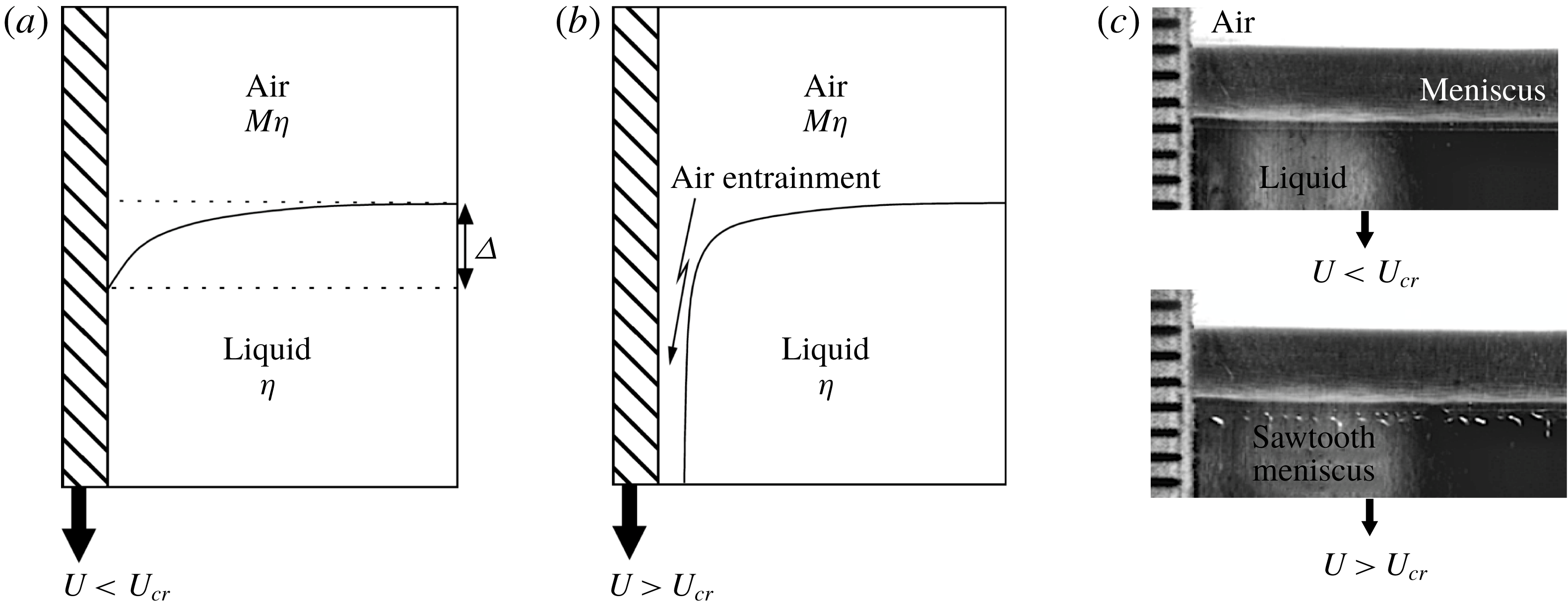
The dip coating process is commonly used in industry to coat solids with a liquid: an object is dragged into a viscous liquid at speed so that it becomes covered by the liquid. If the solid is dragged too fast, a thin film of air will be entrained between the liquid and the solid, and the coating is no longer continuous: this is known as wetting failure (Quéré Reference Quéré1999; Weinstein & Ruschak Reference Weinstein and Ruschak2004); see figure 1. To be able to coat as quickly as possible, one wants to operate at the highest speeds possible without wetting failure occurring; in other words, we are interested in the critical speed
 $U_{cr}$
above which air is entrained. In particular, how does this speed depend on material parameters of the system?
A sketch of the transition to air entrainment produced by a plate descending vertically into a liquid bath. Below the transition (a), the interface meets the solid at a contact line, above which the solid is dry, and below which it is covered with liquid. Above the transition (b), a thin film of air has been entrained. (c) Shows an experiment example of a quasi-steady interface before and after the transition to air entrainment, taken from Vandre, Carvalho & Kumar (Reference Vandre, Carvalho and Kumar2013). At the lower edge of the entrained sheet, sawtooth-shaped instabilities are often observed.
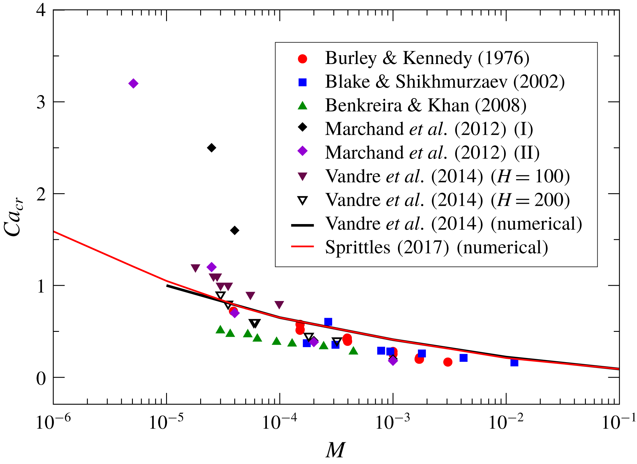
Simulations and experimental data of
 $Ca_{cr}$
for different
 $M$
. The experimental data are taken: from Vandre, Carvalho & Kumar (Reference Vandre, Carvalho and Kumar2014) for a glycerol–air experimental set-up with
 $\unicode[STIX]{x1D703}_{e}\approx 81^{\circ }$
and baths of different widths
 $H$
(
 $\unicode[STIX]{x03BC}\text{m}$
); from Marchand et al. (Reference Marchand, Chan, Snoeijer and Andreotti2012) for a silicone oil–air set-up with
 $\unicode[STIX]{x1D703}_{e}\approx (51^{\circ },57^{\circ })$
for either (I) the measured speed at which rupture of the free interface is first seen or (II) the speed of the growth of the rewetting ridge; from Benkreira & Khan (Reference Benkreira and Khan2008) for a silicone oil–air set-up (
 $\unicode[STIX]{x1D703}_{e}\approx 60^{\circ }$
); from Burley & Kennedy (Reference Burley and Kennedy1976); and from Blake & Shikhmurzaev (Reference Blake and Shikhmurzaev2002). The numerical data are from Sprittles (Reference Sprittles2017) and Vandre et al. (Reference Vandre, Carvalho and Kumar2014), with
 $\unicode[STIX]{x1D703}_{e}=90^{\circ }$
in both cases.
To address this problem systematically, many experimental studies (Blake & Ruschak Reference Blake and Ruschak1979; Benkreira & Khan Reference Benkreira and Khan2008; Benkreira & Ikin Reference Benkreira and Ikin2010; Marchand et al.
Reference Marchand, Chan, Snoeijer and Andreotti2012; Vandre, Carvalho & Kumar Reference Vandre, Carvalho and Kumar2012; Vandre et al.
Reference Vandre, Carvalho and Kumar2014) have considered an idealized configuration in which a solid plate is pulled at speed
 $U$
into a large bath of liquid of viscosity
 $\unicode[STIX]{x1D702}$
(see figure 2), making the problem close to two-dimensional. Below the critical speed, a contact line separates the dry half of the solid above from the wetted half, which in the steady state is at a depth
 $\unicode[STIX]{x1D6E5}$
below the level of the bath. Above the critical speed, a thin layer of air (or another gas) is entrained, whose shape depends on the way the experiment is conducted. One final state that is observed frequently is that of the contact line assuming an irregular unsteady sawtooth shape (Blake & Ruschak Reference Blake and Ruschak1979), also seen in figure 1(c). Our focus will be to calculate the critical speed
 $U_{cr}$
, using a two-dimensional description. The complicated three-dimensional, and usually unsteady, state past this transition is beyond the scope of the present paper.
As recorded in figure 2, many experiments and simulations have determined
 $U_{cr}$
as a function of the viscosity ratio
 $M=\unicode[STIX]{x1D702}_{g}/\unicode[STIX]{x1D702}$
, which is the most important control parameter, where
 $\unicode[STIX]{x1D702}_{g}$
is the viscosity of the gas. Assuming that the transition arises from a competition of viscous forces and surface tension forces, the plate speed is represented in dimensionless form as a capillary number
 $Ca=\unicode[STIX]{x1D702}U/\unicode[STIX]{x1D6FE}$
, where
 $\unicode[STIX]{x1D6FE}$
is the surface tension of the liquid–air interface. Plotting
 $Ca_{cr}$
as a function of
 $M$
, one finds a consistent weak dependence on
 $M$
, more or less independent of other parameters, such as the equilibrium contact angle
 $\unicode[STIX]{x1D703}_{e}$
(Bonn et al.
Reference Bonn, Eggers, Indekeu, Meunier and Rolley2009). Here and for the rest of this paper, we will make no attempt to account for a speed-dependent contact angle on a microscopic scale, using
 $\unicode[STIX]{x1D703}_{e}$
to define the interface slope at the solid substrate. Other dip coating experiments (e.g. Burley & Kennedy Reference Burley and Kennedy1976; Blake & Shikhmurzaev Reference Blake and Shikhmurzaev2002) also agree with this trend. An exception are the recent data of Marchand et al. (Reference Marchand, Chan, Snoeijer and Andreotti2012), who for small values of
 $M$
found somewhat larger critical capillary numbers. The reason for this discrepancy is not understood.
Included in figure 2 are also recent numerical simulations (Vandre et al. Reference Vandre, Carvalho and Kumar2014; Sprittles Reference Sprittles2015), which agree well with experimental data – see also Vandre et al. (Reference Vandre, Carvalho and Kumar2014) for direct comparisons between simulation and experiment for specific geometries and fluid parameters. Key to this success was the development of finite element methods (FEMs) with sufficiently high resolution near the contact line, such that length scales down to approximately 1 nm can be resolved (Sprittles Reference Sprittles2015). Thus we are able to focus our theoretical efforts on the relatively simple hydrodynamic description used in some simulations: the two-dimensional Stokes equation, which neglects inertia. This assumes that the fluid is sufficiently viscous for the Reynolds number to be small; even if this is not the case, the local Reynolds number based on flow features near the contact line is likely to be small. By adopting a two-dimensional description, the contact line is assumed to be straight, and instabilities associated with a wavy contact line are disregarded.
In the simulations considered by us, the contact line singularity (Bonn et al.
Reference Bonn, Eggers, Indekeu, Meunier and Rolley2009; Snoeijer & Andreotti Reference Snoeijer and Andreotti2013) is regularized using a slip length, whose numerical value for a fluid is typically between 1 and 10 nm (Lauga, Brenner & Stone Reference Lauga, Brenner, Stone, Tropea, Foss and Yarin2008). In a gas, on the other hand, the slip length
 $\unicode[STIX]{x1D706}_{g}$
is set by the mean free path (Sprittles Reference Sprittles2017), and thus may be quite different. We thus treat the slip lengths in the liquid and in the gas as separate quantities, although in the particular simulations presented above they are assumed equal. We also assume that the liquid bath is large, and approaches a constant level far from the plate. As a result, the only relevant external length scale is the capillary length
 $l_{c}=\sqrt{\unicode[STIX]{x1D6FE}/\unicode[STIX]{x1D70C}g}$
of the liquid, where
 $\unicode[STIX]{x1D70C}$
is the density of the liquid (the gas density being negligibly small) and
 $g$
is the acceleration due to gravity.
Thus our task is to calculate the critical dimensionless plate speed as a function of four dimensionless parameters:
 $$\begin{eqnarray}\displaystyle Ca_{cr}=Ca_{cr}(M,\unicode[STIX]{x1D703}_{e},\unicode[STIX]{x1D706}/l_{c},\unicode[STIX]{x1D706}_{g}/l_{c}). & & \displaystyle\end{eqnarray}$$
In the case of strong spatial confinement
 $H$
of the bath (Vandre et al.
Reference Vandre, Carvalho and Kumar2014),
 $l_{c}$
would have to be replaced by
 $H$
. This continuum description leaves out kinetic effects (Sprittles Reference Sprittles2017), which come from the gas no longer being in local equilibrium. These effects are a possible explanation for the observed dependence of
 $Ca_{cr}$
on the gas pressure (Benkreira & Khan Reference Benkreira and Khan2008), which otherwise would enter through
 $\unicode[STIX]{x1D706}_{g}$
(Marchand et al.
Reference Marchand, Chan, Snoeijer and Andreotti2012).
Since for a liquid–gas system
 $M$
is typically quite small, we will be interested in the limit of small
 $M$
, for which the critical capillary number becomes of order one, as seen in figure 2. Past theories of dynamic wetting transitions have been based on the idea that the transition is controlled by the stress divergence near a moving contact line, cut off only by the regularizing effect of the slip length (Huh & Scriven Reference Huh and Scriven1971). This idea has been applied to understand the dynamical wetting transition as a solid plate is withdrawn from a liquid bath which wets the plate partially (Eggers Reference Eggers2004, Reference Eggers2005), and for which the effect of the surrounding gas can be neglected. Since viscous stresses in a thin layer of fluid are strong, the transition towards a solid covered by a liquid occurs at small capillary numbers, and is within reach of a small-capillary-number expansion. Subsequently it was shown that the transition occurs by way of a saddle-node bifurcation (Snoeijer et al.
Reference Snoeijer, Andreotti, Delon and Fermigier2007b
; Chan, Snoeijer & Eggers Reference Chan, Snoeijer and Eggers2012), such that no solution exists above a critical speed.
In the present case of a plate plunging into a bath, interface angles are no longer small, so previous authors (Cox Reference Cox1986; Kistler Reference Kistler and Berg1993) have used an expansion for small capillary numbers valid for arbitrary angles (Voinov Reference Voinov1976; Cox Reference Cox1986), based on the Huh & Scriven (Reference Huh and Scriven1971) solution for the viscous flow in a wedge. This yields the interface angle
 $\unicode[STIX]{x1D703}_{d}$
(sometimes referred to as the dynamical or apparent contact angle) at a given distance
 $l_{d}$
from the contact line in terms of the equilibrium angle, evaluated at a microscopic distance from the contact line, set by the slip length. Similar approaches, based on a local balance between capillary, viscous and contact line forces, have been employed subsequently (Duez et al.
Reference Duez, Ybert, Clanet and Bocquet2007; Ledesma-Aguilar, Hernández-Machado & Pagonabarraga Reference Ledesma-Aguilar, Hernández-Machado and Pagonabarraga2013; Vandre et al.
Reference Vandre, Carvalho and Kumar2013) to describe entrainment speeds in both experiment and numerical simulation. Cox (Reference Cox1986) proposed that a transition occurs when
 $\unicode[STIX]{x1D703}_{d}$
has reached
 $180^{\circ }$
, although the underlying theory breaks down in that limit, as does the assumption of small capillary number. Using a constant value of
 $l_{d}$
, this predicts a logarithmic dependence of
 $Ca_{cr}$
, which appears to be qualitatively consistent with figure 2. However, to fit the data properly,
 $l_{d}$
has to be adjusted (Duez et al.
Reference Duez, Ybert, Clanet and Bocquet2007; Ledesma-Aguilar et al.
Reference Ledesma-Aguilar, Hernández-Machado and Pagonabarraga2013; Vandre et al.
Reference Vandre, Carvalho and Kumar2013), while
 $l_{d}$
should really be determined self-consistently by the theory.
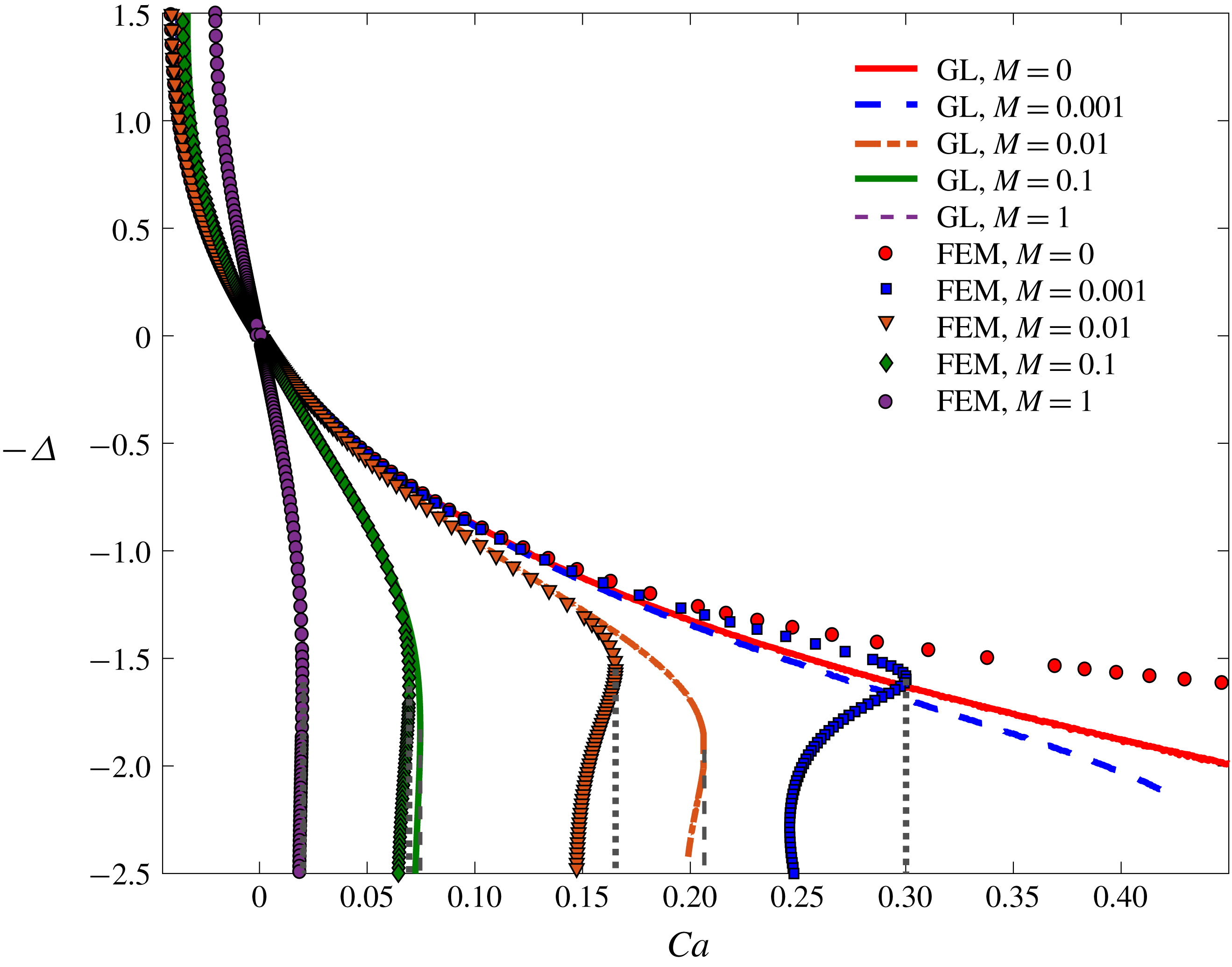
Bifurcation curves as obtained from FEM simulations for
 $\unicode[STIX]{x1D703}_{e}=\unicode[STIX]{x03C0}/2$
and different viscosity ratio
 $M$
, compared to results of the GL approximation (A 1); the slip length is
 $\unicode[STIX]{x1D706}=10^{-5}$
. The vertical lines represent the location of
 $Ca_{cr}$
for the FEM simulation (dotted) and the GL approximation (dashed). The upper branch is stable, the lower unstable. For small
 $M$
, the GL approximation bifurcates at much larger values of
 $Ca$
than predicted by numerical simulation.
To deal with this problem, Snoeijer (Reference Snoeijer2006) has generalized Cox’s (Reference Cox1986) description to include gravity and the effect of boundary conditions into the theory in a self-consistent fashion, valid for small
 $Ca$
, resulting in a theory free of adjustable parameters apart from the slip length, which is included in a phenomenological fashion (Chan et al.
Reference Chan, Srivastava, Marchand, Andreotti, Biferale, Toschi and Snoeijer2013). In appendix A, we describe an improved theory which removes the remaining freedom with regards to slip for contact angles close to
 $90^{\circ }$
. The resulting description is known as the ‘generalized lubrication’ (GL) approximation. It is written as a differential equation for the interface angle
 $\unicode[STIX]{x1D703}$
, which can be solved numerically by shooting from the known contact angle
 $\unicode[STIX]{x1D703}_{e}$
at the contact line towards a horizontal bath. In figure 3, the result is compared with FEM simulations for various values of
 $M$
. The depression of the contact line position below the bath is denoted by
 $\unicode[STIX]{x1D6E5}$
(as defined in figure 1
a), and plotted as a function of
 $Ca$
.
FEM simulations (to be described in somewhat more detail below) are set up to find stationary states, both stable and unstable. As the capillary number increases from zero,
 $\unicode[STIX]{x1D6E5}$
increases, until a maximum value
 $Ca_{cr}$
of the capillary number is found, where the saddle-node bifurcation is taking place. The upper branch corresponds to stable states, which are observed experimentally, while the lower branch is unstable, along which in a time-dependent simulation
 $\unicode[STIX]{x1D6E5}$
continues to increase to dynamically dry the solid. This structure agrees with that found analytically and computationally for the withdrawal of a plate (Chan et al.
Reference Chan, Snoeijer and Eggers2012). Indeed, as long as
 $M$
is of the order of one or larger, the critical capillary number is small and the GL approximation describes the entire bifurcation curve well. However, as
 $M$
decreases, the agreement deteriorates. Even for
 $M=10^{-2}$
, there is qualitative agreement, which might explain the success of local theories (Duez et al.
Reference Duez, Ybert, Clanet and Bocquet2007; Ledesma-Aguilar et al.
Reference Ledesma-Aguilar, Nistal, Hernández-Machado and Pagonabarraga2011, Reference Ledesma-Aguilar, Hernández-Machado and Pagonabarraga2013) to explain experimental observations at moderate viscosity ratios. However, beyond
 $M=10^{-2}$
, the GL approximation far overpredicts
 $Ca_{cr}$
, and for
 $M=10^{-3}$
, we were no longer able to detect a bifurcation in the GL approximation. If a bifurcation still exists within the GL approximation, it would predict a critical capillary number far too large to be realistic. However, if
 $M$
is strictly zero (no gas), there is no transition even in the full FEM numerical simulation, confirming that it is the presence of the gas, trapped in a narrow gap between the liquid and the plate, which drives the transition. In the present paper, we will address the small-
 $M$
region
 $10^{-6}\leqslant M\leqslant 10^{-2}$
, for which traditional theories based on a small-
 $Ca$
expansion fail.
One might think that at least along the upper branch, when the air has not yet become important for small values of
 $M$
, the GL approximation might be a reasonable description of the interface, as the bifurcation curves of figure 3 do not seem to be too far off. However, we will see that the low-capillary-number theory for
 $M=0$
does not describe the shape of the interface correctly even on a qualitative level. Instead, as first suggested by Jacqmin (Reference Jacqmin2002), for
 $Ca\gtrsim 1$
the interface becomes close to a cusp, with an apparent contact angle of
 $180^{\circ }$
. The local solution corresponding to this contact angle was described by Benney & Timson (Reference Benney and Timson1980). However, our simulations show that directly at the contact line the tip is rounded at a very small radius of curvature
 $R$
, similar to a solution found by Jeong & Moffatt (Reference Jeong and Moffatt1992) for a cusped interface created by a bulk flow rather than the presence of a solid wall.
In the following two subsections we will recall the equations being solved numerically, which also form the basis for our analytical description, and briefly describe the numerical method being used. Then § 2 describes the solution for the case
 $M=0$
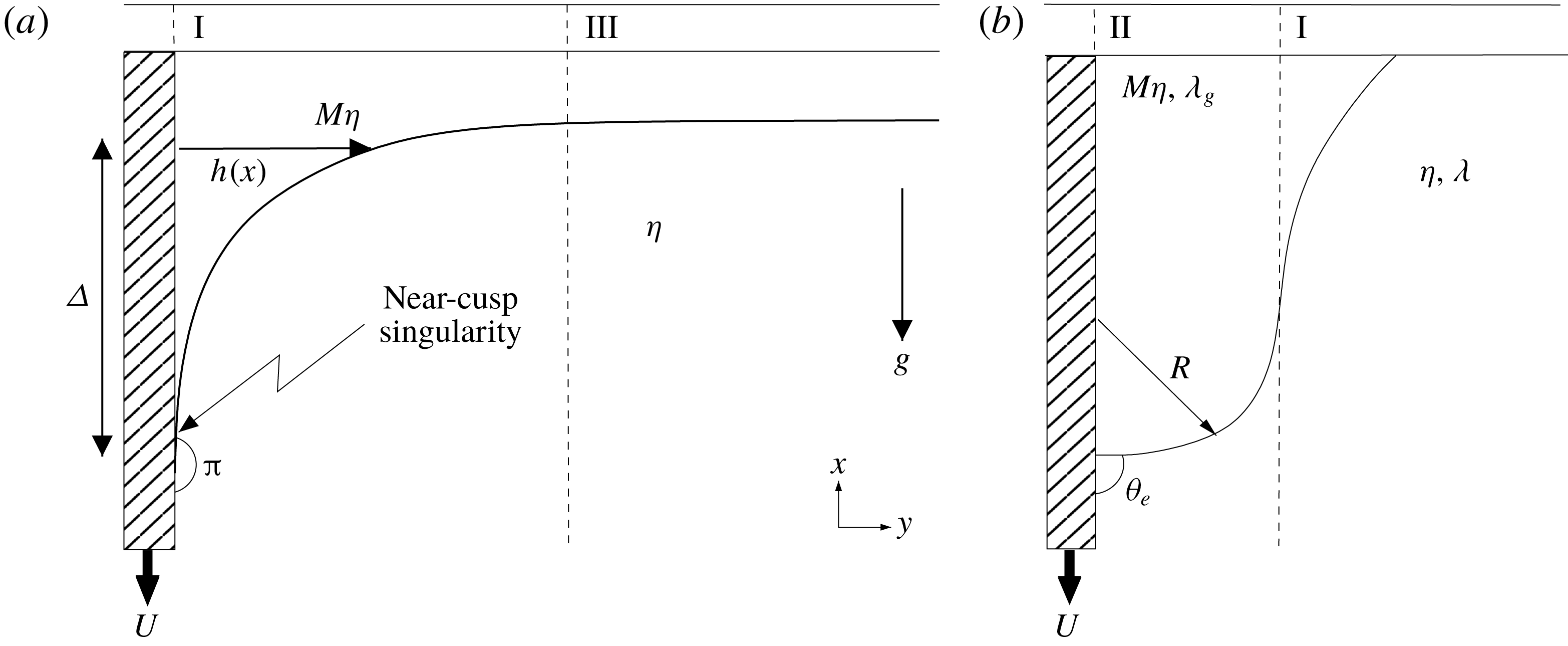
(no gas), in which case there is no transition. We show that the solution can be broken up into three different regions (see figure 4). These are the cusp (region I), described by Benney & Timson’s (Reference Benney and Timson1980) solution, and the tip (region II), which regularizes the cusp tip on a scale
 $R$
. The large-scale behaviour is described by the bath solution (region III), which asymptotes to a flat interface. In § 3 we show how, even for small
 $M$
, the gas trapped inside the cusp region drives a transition.
1.1 Theoretical formulation
Consider the steady two-dimensional, two-phase Stokes flow generated by a plate plunging at speed
 $U$
into a liquid bath in a direction aligned with the gravitational field (see figure 4); we assume that the bath is semi-infinite. The superscripts
 $[\;]^{l,g}$
are used to distinguish the quantity ‘
 $[\;]$
’ for the liquid and gas, respectively.
A sketch of a plate plunging vertically into a bath. On some outer scale (a), a near-cusp forms between the liquid interface and plate. This is the cusp region (I). Assuming the bath to be very wide compared to
 $\unicode[STIX]{x1D6E5}$
(the distance from the contact line to the bath), the interface eventually becomes very flat. This is represented by the bath region (III). On some inner scale,
 $R$
, the cusp must round and make contact with the plate (b). This is known as the contact line region (II). The numbering reflects the order in which the zones are analysed.
Neglecting inertial effects, both fluids satisfy the incompressible Stokes equation,
 $$\begin{eqnarray}\displaystyle \unicode[STIX]{x1D735}\boldsymbol{\cdot }\boldsymbol{u}^{l,g}=0,\quad \unicode[STIX]{x1D702}^{l,g}\unicode[STIX]{x1D6FB}^{2}\boldsymbol{u}^{l,g}=\unicode[STIX]{x1D735}p^{l,g}-\unicode[STIX]{x1D70C}^{l,g}\boldsymbol{g}, & & \displaystyle\end{eqnarray}$$
where
 $\boldsymbol{g}$
is the acceleration due to gravity and the stress of each fluid is defined by
 $$\begin{eqnarray}\displaystyle \unicode[STIX]{x1D70E}_{ij}^{l,g}=-\unicode[STIX]{x1D6FF}_{ij}p^{l,g}+\unicode[STIX]{x1D702}^{l,g}e_{ij}^{l,g},\quad e_{ij}^{l,g}=\frac{\unicode[STIX]{x2202}u_{i}^{l,g}}{\unicode[STIX]{x2202}x_{j}}+\frac{\unicode[STIX]{x2202}u_{j}^{l,g}}{\unicode[STIX]{x2202}x_{i}}. & & \displaystyle\end{eqnarray}$$
This system of equations (1.2) for both flows is solved subject to kinematic and dynamic boundary conditions at the interface (
 $y=h(x)$
with normal
 $\boldsymbol{n}$
and tangent
 $\boldsymbol{t}$
):
 $$\begin{eqnarray}\displaystyle \left.\begin{array}{@{}c@{}}\displaystyle \boldsymbol{u}^{l}\boldsymbol{\cdot }\boldsymbol{t}=\boldsymbol{u}^{g}\boldsymbol{\cdot }\boldsymbol{t},\quad \boldsymbol{u}^{l}\boldsymbol{\cdot }\boldsymbol{n}=\boldsymbol{u}^{g}\boldsymbol{\cdot }\boldsymbol{n}=0,\quad \boldsymbol{n}\boldsymbol{\cdot }\unicode[STIX]{x1D748}^{l}\boldsymbol{\cdot }\boldsymbol{t}=\boldsymbol{n}\boldsymbol{\cdot }\unicode[STIX]{x1D748}^{g}\boldsymbol{\cdot }\boldsymbol{t},\\ \displaystyle \boldsymbol{n}\boldsymbol{\cdot }\unicode[STIX]{x1D748}^{l}\boldsymbol{\cdot }\boldsymbol{n}-\boldsymbol{n}\boldsymbol{\cdot }\unicode[STIX]{x1D748}^{g}\boldsymbol{\cdot }\boldsymbol{n}=-\unicode[STIX]{x1D6FE}\unicode[STIX]{x1D705}\equiv -\unicode[STIX]{x1D6FE}\frac{\text{d}^{2}h}{\text{d}x^{2}}\left[1+\left(\frac{\text{d}h}{\text{d}x}\right)^{2}\right]^{-3/2}.\end{array}\right\} & & \displaystyle\end{eqnarray}$$
The far-field conditions of a semi-infinite bath imply that
 $$\begin{eqnarray}\displaystyle y\rightarrow \infty ,\quad |\boldsymbol{u}^{l,g}|\rightarrow 0. & & \displaystyle\end{eqnarray}$$
At the plate, the no-slip boundary condition leads to the ‘moving contact line singularity’ (Huh & Scriven Reference Huh and Scriven1971). In order for the contact line to be able to move over the solid, we allow the fluid to move with respect to the solid, at a speed proportional to the shear rate; this is the Navier slip law (Navier Reference Navier1827; Lauga et al.
Reference Lauga, Brenner, Stone, Tropea, Foss and Yarin2008). Defining the velocity of the fluid to be
 $\boldsymbol{u}^{l,g}=u^{l,g}\boldsymbol{e}_{x}+v^{l,g}\boldsymbol{e}_{y}$
, the Navier slip law is, at
 $y=0$
,
 $$\begin{eqnarray}\displaystyle v^{l,g}=0,\quad u^{l}+U=\unicode[STIX]{x1D706}\frac{\unicode[STIX]{x2202}u^{l}}{\unicode[STIX]{x2202}y},\quad u^{g}+U=\unicode[STIX]{x1D706}_{g}\frac{\unicode[STIX]{x2202}u^{g}}{\unicode[STIX]{x2202}y}, & & \displaystyle\end{eqnarray}$$
where
 $\unicode[STIX]{x1D706}$
and
 $\unicode[STIX]{x1D706}_{g}$
are the slip lengths in the liquid and in the gas, respectively. From here on, we will make all lengths dimensionless using
 $l_{c}$
, unless stated. At the contact line, we impose a fixed contact angle, disregarding non-equilibrium effects on the scale of the slip length:
 $$\begin{eqnarray}\displaystyle \frac{\unicode[STIX]{x2202}h}{\unicode[STIX]{x2202}x}=-\tan \unicode[STIX]{x1D703}_{e}. & & \displaystyle\end{eqnarray}$$
The above system of equations defines a stationary state of the problem, which is defined by the vanishing of normal velocities with respect to the interface or, equivalently, the interface being a streamline. The dimensionless numbers determining this problem are
 $Ca,~M,~\unicode[STIX]{x1D706}/l_{c}$
and
 $\unicode[STIX]{x1D706}_{g}/l_{c}$
.
1.2 Numerical formulation
We perform numerical simulations of (1.2)–(1.7) using the FEM, in order to find stationary states, as described in Sprittles & Shikhmurzaev (Reference Sprittles and Shikhmurzaev2012) and Sprittles (Reference Sprittles2015). The method is based on an arbitrary Lagrangian Eulerian mesh design which allows for the free surface to be captured with high accuracy. The domain size is made large enough so as not to affect the contact line dynamics. About the contact line, the mesh is graded with small elements to enable the dynamics of the flow on the scale of the slip length, and below, to be captured alongside the bulk flow where larger elements are permitted. The above set of equations are solved for in the domain, except for the far-field boundary condition (1.5), which would require an infinite domain. Instead, a boundary is located at a fixed ‘large’ distance from the contact line where the boundary conditions
 $\boldsymbol{u}\boldsymbol{\cdot }\boldsymbol{e}_{x}=0$
, no tangential stress at the interface and a perpendicular flat interface are set, equivalent to what one would expect at a plane of symmetry.
In simulations, the domain is taken to be a closed rectangle with dimensionless width of up to
 $H_{b}=10^{3}$
and depth
 $D=10$
above and below the otherwise flat interface. The slip length is chosen to compare to FEM simulations performed by Vandre et al. (Reference Vandre, Carvalho and Kumar2012),
 $\unicode[STIX]{x1D706}=\unicode[STIX]{x1D706}_{g}=10^{-4}$
, and benchmark calculations in Sprittles (Reference Sprittles2015) confirm excellent agreement between the two codes. Simulations are performed for
 $\unicode[STIX]{x1D703}_{e}=\unicode[STIX]{x03C0}/2$
unless otherwise stated. This can be compared to the estimated values of
 $\unicode[STIX]{x1D703}_{e}$
found for the experimental samples in the caption for figure 2. To find the bifurcation point,
 $M$
is held fixed while the distance from the contact line to the flat bath,
 $\unicode[STIX]{x1D6E5}$
, slowly increases. For each new
 $\unicode[STIX]{x1D6E5}$
, the speed of the plate
 $Ca$
is found. Continuing to increase
 $\unicode[STIX]{x1D6E5}$
, a bifurcation plot, as shown in figure 3, is obtained. This captures the unstable branch of the solution, which cannot be obtained by increasing
 $Ca$
and finding
 $\unicode[STIX]{x1D6E5}$
.
As
 $Ca$
increases past unity, calculations become significantly more challenging, even for
 $M=0$
. Our findings (cf. figure 10) will rationalize such observations by showing that the radius of curvature at the contact line scales with the slip length multiplied by an exponential of
 $-Ca$
. Interestingly then, even at moderate
 $Ca$
, the bottleneck to calculations is in resolving the interface’s curvature
 $R$
and not just the scale of the slip length
 $\unicode[STIX]{x1D706}$
, thus making computational requirements even more tough than already thought and calling into doubt the ‘well-resolvedness’ of many high-
 $Ca$
simulations.
Furthermore, for non-zero
 $M$
, as
 $Ca$
gets increasingly large, resolving past the bifurcation point onto the unstable branch of the solution eventually becomes impossible. One can see how sharp the turning from one branch onto the other is becoming even at smaller
 $Ca$
by looking at figure 3. Our work will show that this complication occurs because the size of the perturbation from the
 $M=0$
solution depends on the magnitude of the velocity of the gas, which (we will show in § 3) scales with
 $M$
. Thus, since a larger
 $Ca_{cr}$
corresponds to a smaller
 $M$
, the perturbation from the
 $M=0$
solution will be smaller, and consequently more difficult to capture numerically. Accurate resolution about the contact line thus rapidly gets increasingly hard for greater
 $Ca$
, and as a result, we restrict the analysis of numerical simulations to plate speeds
 $Ca\leqslant 2.51$
. The need for an accurate analytical theory of the bifurcation for very small
 $M$
thus becomes even more apparent. We will see that
 $Ca\gtrsim 0.5$
can already be considered ‘large’, and will be successfully described by an expansion for large capillary numbers.
The interface for
 $Ca=1.04$
and
 $M=0$
(solid line),
 $M=1.5\times 10^{-6}$
(dot-dashed line) and
 $M=10^{-5}$
(dashed line). On the macroscale, the interface approaches a
 $180^{\circ }$
contact angle, but bends on some inner scale towards
 $\unicode[STIX]{x1D703}_{e}=\unicode[STIX]{x03C0}/2$
, as seen in the inset. On the macroscale there is little difference as
 $M$
increases; only on some intermediate scale about the contact line (shown in the inset) can the effect of a finite
 $M$
be seen.
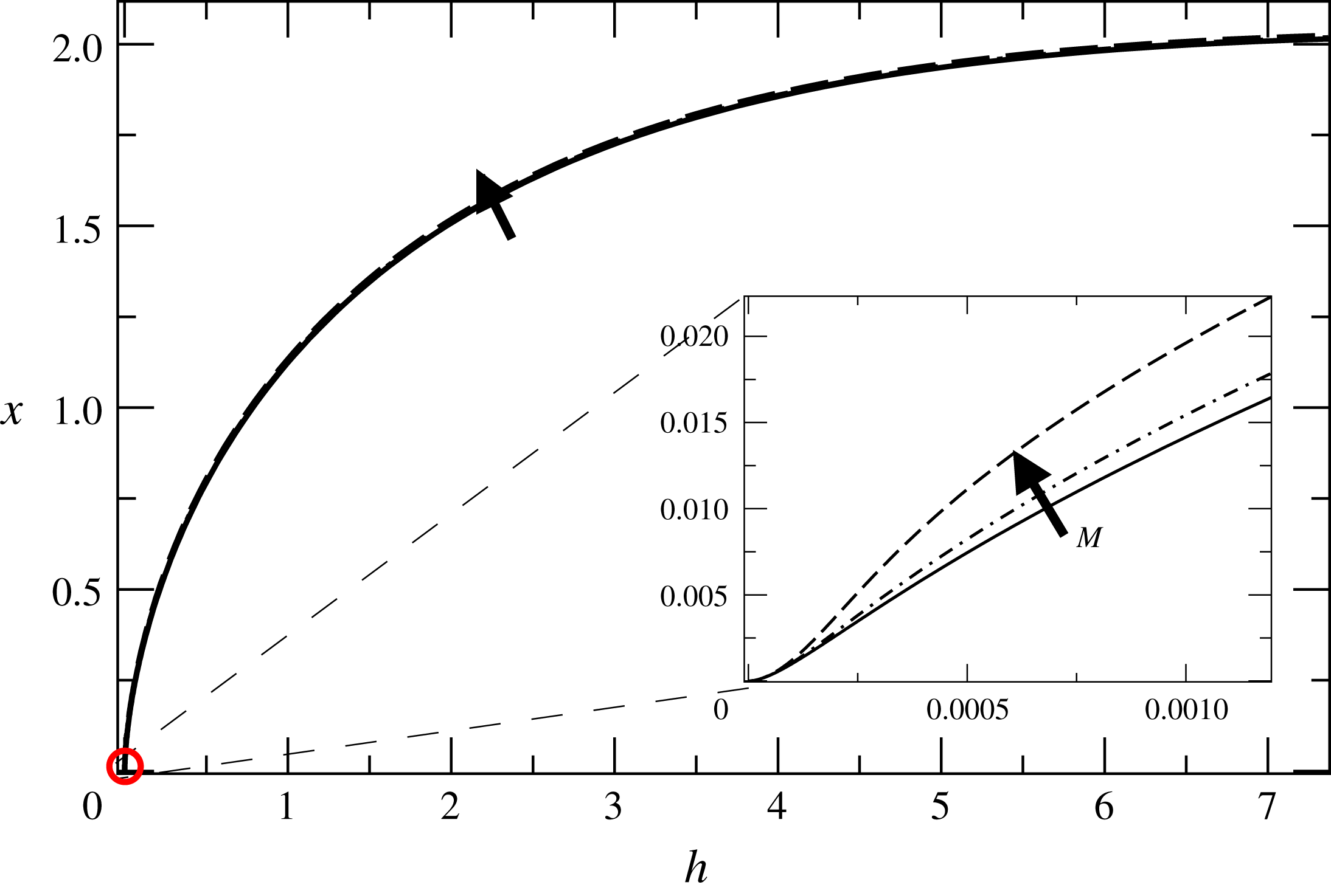
Typical results for the interface shape as found from numerical simulations are shown in figure 5 at
 $Ca\approx 1$
. As illustrated in the schematic sketch of figure 4, on the macroscale the interface approaches a cusp, which makes a
 $180^{\circ }$
apparent contact angle with the plate, so that the liquid flow becomes parallel to the plate. We show the stationary profiles for
 $M=0$
,
 $M=10^{-6}$
and
 $M=10^{-5}$
, close to the bifurcation at which air entrainment occurs. However, even close to the bifurcation, the interface shape hardly changes. This observation forms the basis of our approach: below in § 2 we first calculate the interface for
 $M=0$
, and then (see § 3) treat the presence of air as a small perturbation in order to calculate the bifurcation.
This is illustrated in the inset of figure 5, which shows a highly enlarged region around the contact line. At some very small inner scale (which will be discussed in more detail in § 2.2 below), the interface turns to make contact with the plate at
 $\unicode[STIX]{x1D703}=\unicode[STIX]{x1D703}_{e}$
. Only at an intermediate scale, seen in the inset, is there a noticeable change of the interface shape with
 $M$
.
2 The interface in the absence of gas
A sketch of the different regions introduced to analyse the problem is shown in figure 4. On a macroscopic scale (figure 4
a), the contact angle is close to
 $180^{\circ }$
, since
 $U$
(or more specifically
 $Ca$
) is very large, and drags down the interface. This produces a cusp shape (which we call region I), which dominates the flow close to the plate. This part of the flow is governed by viscous and surface tension forces. Eventually the interface must level off towards the bath, so there is another region (region III), which is dominated by viscous forces and gravity. However, as one comes close to the plate, the interface must meet the plate at a prescribed contact angle
 $\unicode[STIX]{x1D703}_{e}$
as shown on figure 4(b). This necessitates the existence of another region (region II) near the tip.
2.1 Region I: the cusp singularity
At very high speeds, the interface is bent so severely that it appears to meet the plate tangentially, at an apparent contact angle
 $\unicode[STIX]{x1D703}_{e}=\unicode[STIX]{x03C0}$
. We describe this situation using the asymptotic solution of the contact line problem of Benney & Timson (Reference Benney and Timson1980) for
 $M=0$
and
 $\unicode[STIX]{x1D703}_{e}=\unicode[STIX]{x03C0}$
, and assuming a no-slip boundary condition. This is appropriate for our case, as we are on an intermediate scale excluding the contact line region. Since the interface is parallel to the plate at the contact line, the contact line singularity is weakened and the local energy dissipation remains finite, as we will see. As a result, the paradox discovered by Huh & Scriven (Reference Huh and Scriven1971) does not exist, although the curvature does still diverge.
For
 $\unicode[STIX]{x1D703}_{e}=\unicode[STIX]{x03C0}$
, since viscous stresses dominate gravitational effects about the contact line, the liquid phase is described by the Stokes equation (1.2) with
 $g=0$
. This is equivalent to solving the biharmonic equation for the streamfunction
 $\unicode[STIX]{x1D713}$
, represented in polar coordinates
 $(r,\unicode[STIX]{x1D719})$
, defined in figure 6(a),
 $$\begin{eqnarray}\displaystyle \unicode[STIX]{x0394}^{2}\unicode[STIX]{x1D713}=0,\quad u_{r}=\frac{1}{r}\frac{\unicode[STIX]{x2202}\unicode[STIX]{x1D713}}{\unicode[STIX]{x2202}\unicode[STIX]{x1D719}},\quad u_{\unicode[STIX]{x1D719}}=-\frac{\unicode[STIX]{x2202}\unicode[STIX]{x1D713}}{\unicode[STIX]{x2202}r}, & & \displaystyle\end{eqnarray}$$
subject to the boundary conditions
 $$\begin{eqnarray}\displaystyle \left.\begin{array}{@{}rcl@{}}\unicode[STIX]{x1D719}=\unicode[STIX]{x03C0}: & \quad & \unicode[STIX]{x1D713}=0,\quad u_{r}=Ca,\\ \unicode[STIX]{x1D719}=g(r): & \quad & \unicode[STIX]{x1D713}=0,\quad \boldsymbol{n}\boldsymbol{\cdot }\unicode[STIX]{x1D748}\boldsymbol{\cdot }\boldsymbol{n}=-\unicode[STIX]{x1D705},\quad \boldsymbol{n}\boldsymbol{\cdot }\unicode[STIX]{x1D748}\boldsymbol{\cdot }\boldsymbol{t}=0.\end{array}\right\} & & \displaystyle\end{eqnarray}$$
Here we have written velocities in units of the capillary speed
 $\unicode[STIX]{x1D6FE}/\unicode[STIX]{x1D702}$
, stress in units of
 $\unicode[STIX]{x1D6FE}/l_{c}$
, and
 $\unicode[STIX]{x1D705}$
, the curvature of the interface, in units of
 $1/l_{c}$
. This corresponds to the no-slip boundary conditions at the plate, the dynamical stress conditions at the liquid–vacuum interface, and a further condition that the liquid–vacuum interface and the liquid–solid interface are streamlines, where the dividing streamline is taken to be
 $\unicode[STIX]{x1D719}=0$
. Benney & Timson (Reference Benney and Timson1980) commit a sign error in front of the curvature term which does not affect their method of calculation, but of course invalidates their results. Ngan & Dussan V. (Reference Ngan and Dussan V.1984) noticed the sign error, but claim that the corrected results lead to conclusions which are ‘physically meaningless’. Mahadevan & Pomeau (Reference Mahadevan and Pomeau1999) claim to have a found a singularity-free solution, and incorrectly conclude that the interface shape should be regular in the case of a
 $180^{\circ }$
contact angle. Here we hope to set the record straight, and test our conclusions by direct comparison with our numerical simulations.
(a) Sketch of the cusp solution for a
 $180^{\circ }$
contact angle. (b) Solutions of (2.9).
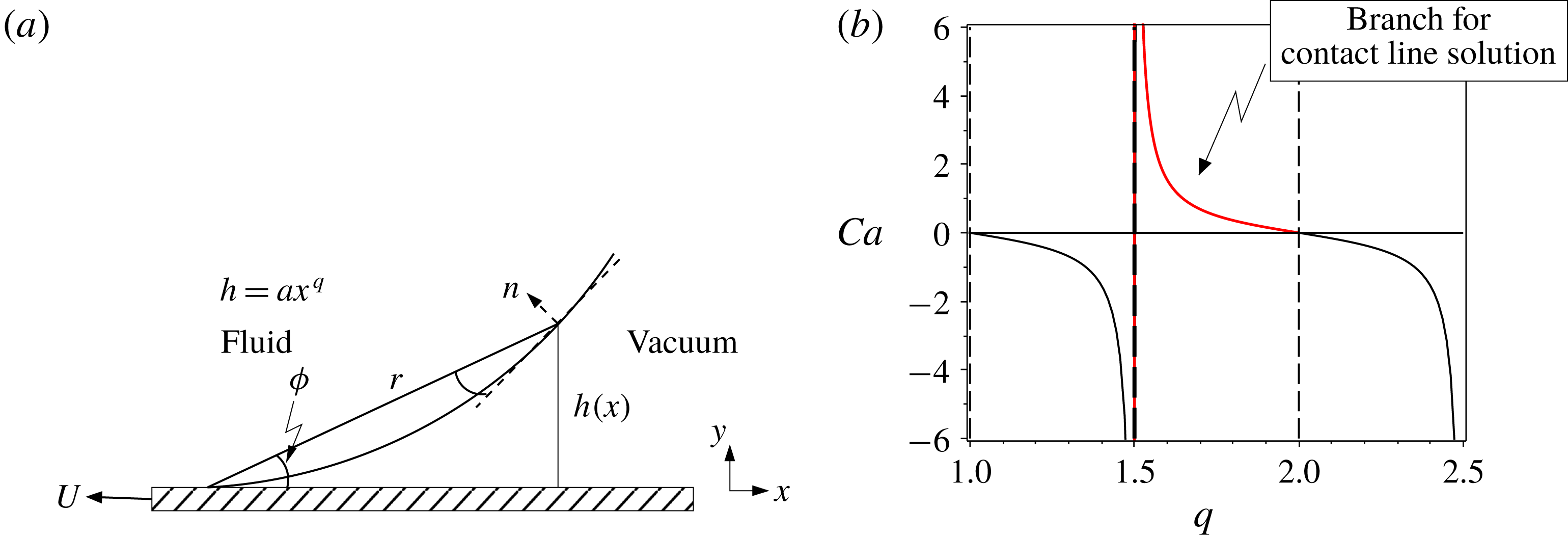
Following Benney & Timson (Reference Benney and Timson1980), we find a similarity solution for this problem, where the free surface, to leading order as one approaches the contact line, has the power-law form
 $$\begin{eqnarray}\displaystyle h(x)=ax^{q}. & & \displaystyle\end{eqnarray}$$
In order to produce a
 $180^{\circ }$
contact angle, we must have
 $q>1$
for consistency.
In the classical calculation of Huh & Scriven (Reference Huh and Scriven1971), (2.1) and (2.2) (with the exception of the normal stress balance) are solved in a wedge, such that
 $h(x)=x\tan \unicode[STIX]{x1D703}$
instead of (2.3). This gives a unique solution for the limit
 $r\rightarrow 0$
, and the normal stress balance will in general not be satisfied. The normal stress balance is then used to calculate corrections to the wedge-shaped interface in a perturbative fashion.
In the present calculation, we use the additional freedom of choosing the exponent
 $q$
in order to satisfy the normal stress balance as well; the value of
 $q$
then results from a solvability condition, which makes this an example of self-similarity of the second kind (Eggers & Fontelos Reference Eggers and Fontelos2015), as opposed to the Huh–Scriven problem, which is of the first kind. The constant
 $a$
in (2.3) sets the amplitude of the solution. In principle, it has to be determined by matching to an outer solution; we will find it below by comparing to the numerical solution.
In polar coordinates
 $(r,\unicode[STIX]{x1D719})$
, see figure 6, the surface becomes
 $\unicode[STIX]{x1D719}=g(r)\approx ar^{q-1}$
. The solution for
 $\unicode[STIX]{x1D713}$
, with a uniform flow
 $-Ca\,\boldsymbol{e}_{x}$
from the downwards velocity of the plate, has the similarity form
 $$\begin{eqnarray}\displaystyle \unicode[STIX]{x1D713}=-Ca\,r\sin \unicode[STIX]{x1D719}+r^{q}F(\unicode[STIX]{x1D719})+O(r^{2q}). & & \displaystyle\end{eqnarray}$$
This will ensure that, to leading order, the interface is the streamline
 $\unicode[STIX]{x1D713}=0$
, as long as
 $F(g(r))\simeq F(0)=a\,Ca$
is satisfied. For
 $\unicode[STIX]{x1D713}$
to be a solution of (2.1),
 $F$
has the form (if
 $q\neq 2$
)
 $$\begin{eqnarray}\displaystyle F(\unicode[STIX]{x1D719})=A\cos q\unicode[STIX]{x1D719}+B\sin q\unicode[STIX]{x1D719}+C\cos (q-2)\unicode[STIX]{x1D719}+E\sin (q-2)\unicode[STIX]{x1D719}, & & \displaystyle\end{eqnarray}$$
where
 $A,~B,~C$
and
 $E$
are unknown constants. To leading order, the curvature is
 $\unicode[STIX]{x1D705}\approx aq(q-1)r^{q-2}$
, and using
 $F(0)=A+C=a\,Ca$
, (2.2) can be written as a system of four homogeneous equations for
 $F$
, for which the determinant is
 $$\begin{eqnarray}\displaystyle \text{Det}=8q(q-1)^{2}(q-2)(\cos q\unicode[STIX]{x03C0})^{2}(2Ca+\tan q\unicode[STIX]{x03C0}). & & \displaystyle\end{eqnarray}$$
For a non-trivial solution to exist, this determinant must vanish. We are interested in solutions such that, in the limit
 $Ca\rightarrow 0$
, the profile converges towards a static meniscus, so that
 $q=2$
. This results in a solution that is regular at the contact line, characterized by finite curvature. Indeed, repeating the above calculation for
 $q=2$
, in which case
 $$\begin{eqnarray}\displaystyle F(\unicode[STIX]{x1D719})=A\cos 2\unicode[STIX]{x1D719}+B\sin 2\unicode[STIX]{x1D719}+C+E\unicode[STIX]{x1D719}, & & \displaystyle\end{eqnarray}$$
the pressure becomes logarithmically singular:
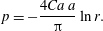 $$\begin{eqnarray}\displaystyle p=-\frac{4Ca\,a}{\unicode[STIX]{x03C0}}\ln r. & & \displaystyle\end{eqnarray}$$
The logarithmic behaviour of the pressure is reminiscent of the logarithmic pressure behaviour of a closing ‘hinged plate’ and a plate in contact with a constant surface stress (Moffatt Reference Moffatt1964). This contradicts Mahadevan & Pomeau’s (Reference Mahadevan and Pomeau1999) claim that the
 $q=2$
solution is singularity-free for any
 $Ca$
. In fact, the normal stress balance is satisfied to leading order only if
 $Ca=0$
.
Instead, to satisfy all boundary conditions (2.2) we make (2.6) vanish by choosing
 $$\begin{eqnarray}\displaystyle \tan (q\unicode[STIX]{x03C0})=-2Ca, & & \displaystyle\end{eqnarray}$$
the branches of which are shown in figure 6. The condition that
 $q=2$
for vanishing
 $Ca$
singles out the branch shown in red, since we expect
 $q$
to decrease with increasing
 $Ca$
, such that the interface curvature increases with increasing speed. Solving for
 $q$
, we find
 $$\begin{eqnarray}\displaystyle q=\frac{\arctan (-2Ca)+2\unicode[STIX]{x03C0}}{\unicode[STIX]{x03C0}}\in \left(\frac{3}{2},2\right]. & & \displaystyle\end{eqnarray}$$
Higher branches correspond to subdominant solutions, while lower branches are unphysical. Our conclusions, to be confirmed by comparison to numerical simulation below, are different from those of Mahadevan & Pomeau (Reference Mahadevan and Pomeau1999) and of Benilov & Vynnycky (Reference Benilov and Vynnycky2013), who find
 $q\geqslant 2$
. For large
 $Ca$
, the power law converges towards
 $q=3/2$
, which is the generic cusp (Eggers & Suramlishvili Reference Eggers and Suramlishvili2017) found for the problem without a solid plate (Jeong & Moffatt Reference Jeong and Moffatt1992).
Since the energy dissipation density
 $\unicode[STIX]{x1D716}$
behaves like the square of a velocity gradient, it is seen from power counting (and confirmed by direct calculation) that
 $\unicode[STIX]{x1D716}\propto r^{2(q-2)}$
, so the total dissipation is finite for
 $q>1$
. This confirms that the usual contact line singularity (Huh & Scriven Reference Huh and Scriven1971) is regularized in the region of interest. To compute the velocity field, we use that
 $A+C=Ca\,a$
, which leads to the streamfunction
 $$\begin{eqnarray}\displaystyle \unicode[STIX]{x1D713} & = & \displaystyle -Ca\,r\sin \unicode[STIX]{x1D719}\nonumber\\ \displaystyle & & \displaystyle +\,ar^{q}\left[\frac{2-q}{2}Ca\cos q\unicode[STIX]{x1D719}+\frac{2-q}{4}\sin q\unicode[STIX]{x1D719}+\frac{q}{2}Ca\cos (q-2)\unicode[STIX]{x1D719}+\frac{q}{4}\sin (q-2)\unicode[STIX]{x1D719}\right].\nonumber\\ \displaystyle & & \displaystyle\end{eqnarray}$$
Plots of FEM profiles of the liquid interface (black curved line) at different
 $Ca$
. The (red) solid straight lines are best fits to the intermediate region
 $h=ax^{q}$
, where
 $q$
is defined by (2.10), and the (red) dashed straight lines are those to the cusp exponent
 $3/2$
. The prefactor
 $a$
(in units of
 $l_{c}$
) is
 $0.76$
and
 $0.49$
, respectively. The best fits are made to approximate the shape of the free surface; the slip length is
 $\unicode[STIX]{x1D706}=10^{-4}$
.
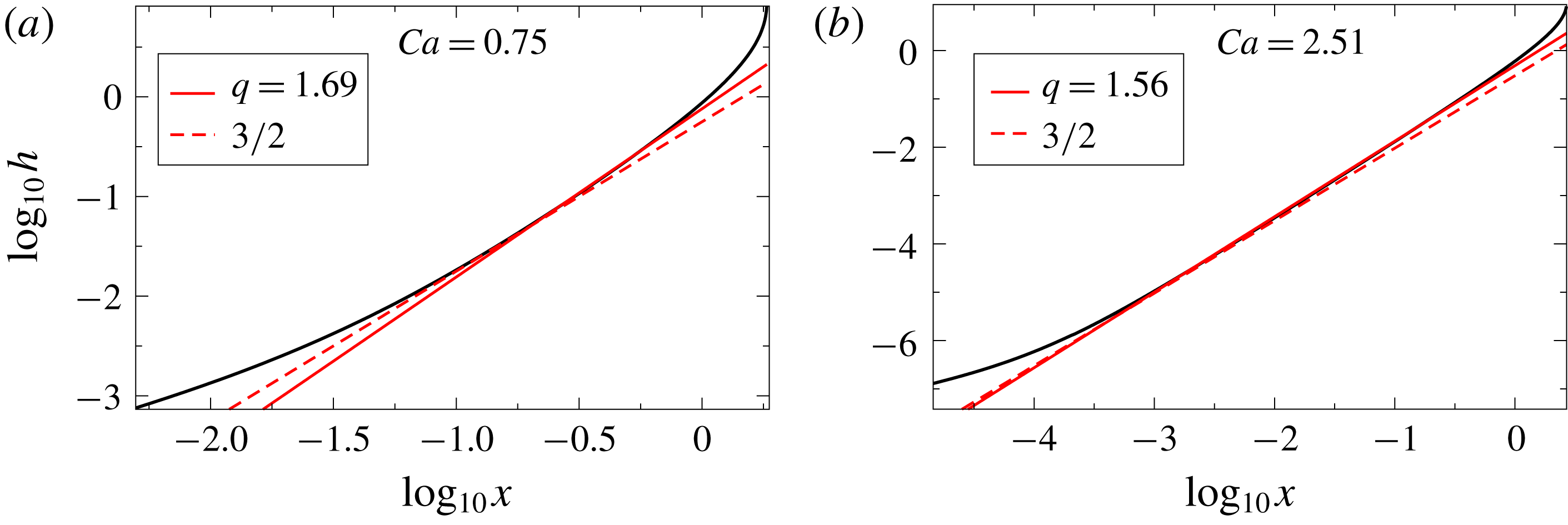
In figure 7 we compare (2.3) and (2.10) to numerical simulations of the full problem for two different values of
 $Ca$
and
 $\unicode[STIX]{x1D703}_{e}=\unicode[STIX]{x03C0}/2$
. For each
 $Ca$
, (2.3) is fitted in a region
 $1\gg h\gg R$
, where the prefactor
 $a$
is used as a fitting parameter (see figure 8). The fits are shown as solid straight lines, while corresponding fits using the asymptotic value
 $q=3/2$
are shown as the dashed straight lines. The quality of the fits increases rapidly with
 $Ca$
, and for
 $Ca=2.51$
the fit is over three decades in
 $x$
. Figure 7 also demonstrates that, while
 $q$
comes quite close to
 $3/2$
(which is the value used by Jacqmin (Reference Jacqmin2002)), the value (2.10) given by theory still provides an improved fit. This demonstrates that
 $a$
is determined as a result of the matching between the solution of Benney & Timson (Reference Benney and Timson1980) and an outer solution. By contrast, Ngan & Dussan V. (Reference Ngan and Dussan V.1984) rejected (2.3) on the grounds that
 $a$
was not determined as part of a local solution.
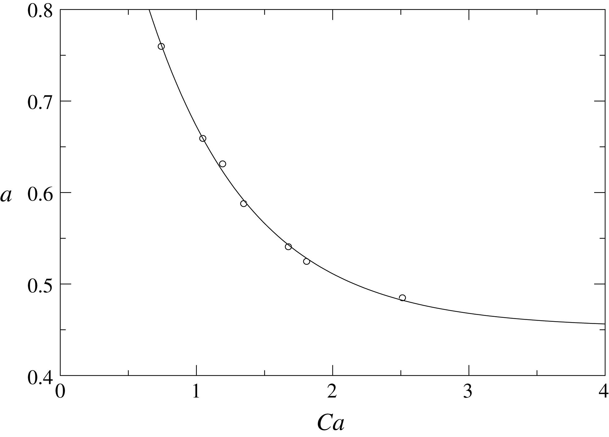
The prefactor
 $a$
in (2.3) as a function of
 $Ca$
. The circles represent values of
 $a$
obtained by fitting (2.3) to numerical simulations as shown in figure 7. The solid line is an empirical fit
 $a=0.45+0.82\exp (-1.31Ca)$
, suggesting that
 $a$
will rapidly approach a finite value as
 $Ca\rightarrow \infty$
.
2.2 Region II: cusp tip and the contact line
We begin by analysing the case
 $\unicode[STIX]{x1D703}_{e}=\unicode[STIX]{x03C0}/2$
. In the case of perfect slip, this would be the same solution as that of no wall, with a line of symmetry at
 $y=0$
. For that case, Jeong & Moffatt (Reference Jeong and Moffatt1992) have found a local similarity solution of the form
 $$\begin{eqnarray}\displaystyle h=\sqrt{2Rx}+ax^{3/2}, & & \displaystyle\end{eqnarray}$$
where
 $a$
is a constant and
 $R$
is the radius of curvature at the tip. The profile (2.12) is the generic form of the singularity of a smooth curve as it is about to make a self-intersection (Eggers & Suramlishvili Reference Eggers and Suramlishvili2017), so we expect it to be valid generically, independent of the flow geometry. In the case of a finite slip length, we now propose on phenomenological grounds that the local cusp solution is
 $$\begin{eqnarray}\displaystyle h=\sqrt{2Rx}+ax^{q}, & & \displaystyle\end{eqnarray}$$
where
 $q$
is the exponent (2.10). Just like the original solution of Jeong & Moffatt (Reference Jeong and Moffatt1992), this can be cast in the similarity form
 $$\begin{eqnarray}\displaystyle h=R^{q/(2q-1)}H(\unicode[STIX]{x1D709}),\quad \unicode[STIX]{x1D709}=R^{1/(1-2q)}x,\quad H(\unicode[STIX]{x1D709})\approx \sqrt{2\unicode[STIX]{x1D709}}+a\unicode[STIX]{x1D709}^{q}. & & \displaystyle\end{eqnarray}$$
This brings out the fact that the cusp solution possesses a single characteristic length scale,
 $R$
.
The composite solution (2.13) (red dashed line) fitted to a FEM simulation of the free surface (black solid line) for two different contact angles;
 $\unicode[STIX]{x1D706}=10^{-4}$
. The fitting parameters are
 $R/\unicode[STIX]{x1D706}\approx 3.4\times 10^{-4}$
and
 $a=0.52$
(a), and
 $R/\unicode[STIX]{x1D706}=0.011$
 $a=0.66$
(b). The inset on the left shows that the composite solution (2.13) slightly underestimates the rate of increase of the interface near the crossover.
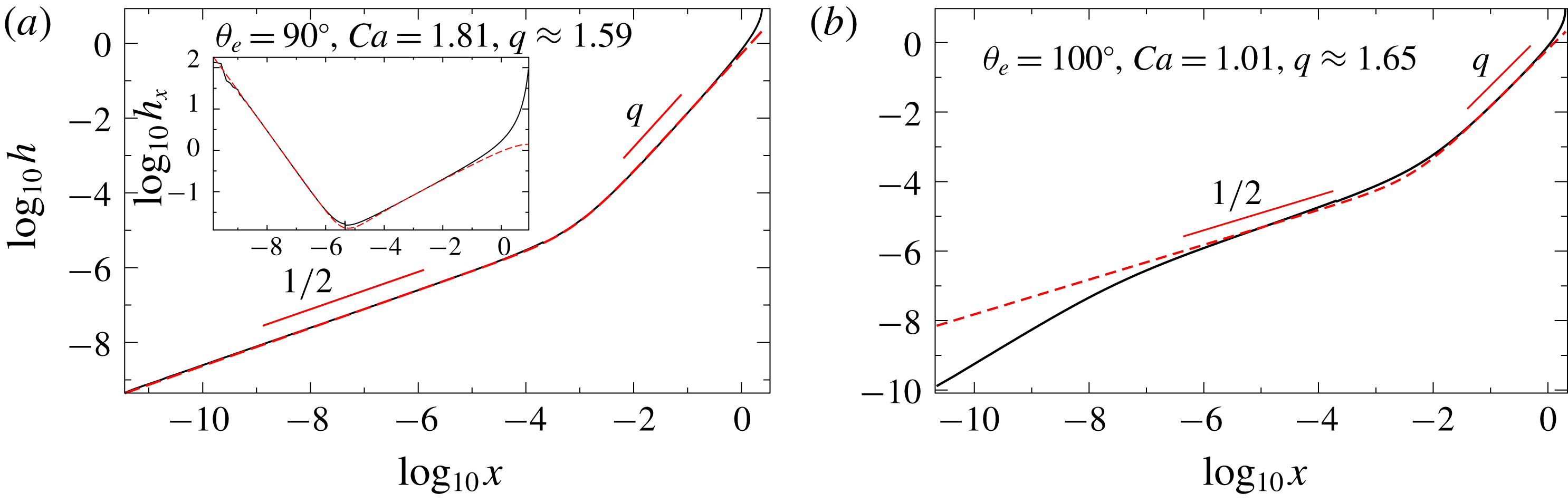
Figure 9(a) shows excellent agreement between our asymptotic description (2.13) and a numerical simulation for
 $\unicode[STIX]{x1D703}_{e}=\unicode[STIX]{x03C0}/2$
. Only when taking the first derivative can a small discrepancy in the crossover region be detected. The adjustable parameters are the amplitude
 $a$
of the cusp solution and the radius of curvature
 $R$
. It is clear that for
 $\unicode[STIX]{x1D703}_{e}\neq \unicode[STIX]{x03C0}/2$
the exponent
 $1/2$
naturally cannot be valid all the way to the contact line. However, figure 9(b) demonstrates that (2.13) is accurate for a remarkable portion of the interface before eventually failing on a very small scale.
This shows that, contrary to the assumptions underlying the conventional theory of the drying transition, the contact line region becomes all but obliterated. Even at modest
 $Ca\approx 1$
the crossover to the contact line region only takes place at a scale of
 $10^{-6}$
, which is two orders of magnitude below the slip length
 $\unicode[STIX]{x1D706}$
. The smallness of
 $R$
in the continuum description raises fundamental questions as to how the contact line region should be modelled in a physical description, to which we return in the discussion (§ 4). We were not able to provide a comparison for larger
 $Ca$
, since we can no longer guarantee that the contact line region is fully resolved. We believe the actual behaviour in the contact line region is not as important as is generally believed, since
 $R$
is the smallest scale that determines the transition. This is at least qualitatively consistent with the conclusions of Eddi, Winkels & Snoeijer (Reference Eddi, Winkels and Snoeijer2013), who find that wetting effects are unimportant for the early stages of drop spreading. Similarly, in Latka et al. (Reference Latka, Boelens, Nagel and de Pablo2018) it was found that the transition to splashing after drop impact on a solid surface is insensitive to the wetting properties of the substrate. The conventional theory of the drying transition based on the Cox–Voinov formula (Cox Reference Cox1986; Kistler Reference Kistler and Berg1993; Vandre et al.
Reference Vandre, Carvalho and Kumar2013) aims to describe how the interface angle increases from
 $\unicode[STIX]{x1D703}_{e}$
to a value close to
 $\unicode[STIX]{x03C0}$
, making a convex shape. However, at the turning point, the interface becomes concave, forming the cusp region, described above. This shows that the conventional theory fails to describe the interface in even a qualitative fashion.
2.2.1 The radius of curvature
 $R$

Returning to the tip region, our main task is to develop a theory for the radius of curvature
 $R$
. This is important, since
 $R$
determines the smallest scale of the cusp into which the gas phase is confined. As a result, in analogy to Eggers (Reference Eggers2001),
 $R$
determines the saddle-node bifurcation if gas is included. In the classical theory of Jeong & Moffatt (Reference Jeong and Moffatt1992) (in the absence of a plate),
 $R$
depends exponentially on the capillary number. In that paper, the authors report an argument by Hinch which represents the cusp tip by a point force of strength
 $2\unicode[STIX]{x1D6FE}$
, which comes from the vertical upward pull of each side of the cusp. At the tip of the cusp, the upward velocity generated by the point force (often called a stokeslet) must cancel the downward velocity along the cusp walls. Since the speed generated by a stokeslet depends logarithmically on the distance in two dimensions, this leads to an exponential dependence of the tip scale on the imposed velocity field.
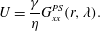
In order to adapt this idea to the present situation, we have to replace the free-space stokeslet with its analogue in the presence of a wall. In order for the tip of the cusp to be stationary, the speed generated at the contact line by a force
 $\boldsymbol{F}=\unicode[STIX]{x1D6FE}\boldsymbol{e}_{x}$
at a distance
 $r$
above the contact line must equal
 $U$
. This is the
 $(x,x)$
component of the Stokes Green function in the presence of a partial-slip wall, assuming that the force is situated on the wall
 $y=0$
:
 $$\begin{eqnarray}\displaystyle U=\frac{\unicode[STIX]{x1D6FE}}{\unicode[STIX]{x1D702}}G_{xx}^{PS}(r,\unicode[STIX]{x1D706}). & & \displaystyle\end{eqnarray}$$
In analogy with the three-dimensional case (Lauga & Squires Reference Lauga and Squires2005), the Green function can be written as the sum of the free-space Green function, its image and a correction factor
 $W_{xx}^{PS}(r,\unicode[STIX]{x1D706})$
. Since the force is on the wall, the image is the same as the Green function itself, and we obtain
 $$\begin{eqnarray}\displaystyle G_{xx}^{PS}(r,\unicode[STIX]{x1D706}) & = & \displaystyle \frac{1}{4\unicode[STIX]{x03C0}}(1-\ln r)+\int _{0}^{\infty }\text{e}^{-u/2}(\ln \hat{r}-1)\,\text{d}u\nonumber\\ \displaystyle & & \displaystyle -\,4\unicode[STIX]{x1D706}^{2}\int _{0}^{\infty }\left(1-\left(1+\frac{1}{2}\right)\text{e}^{-u/2}\right)\frac{1}{\hat{r}^{2}}\,\text{d}u,\quad \hat{r}=\sqrt{x^{2}+(\unicode[STIX]{x1D706}u)^{2}}.\end{eqnarray}$$
The slip length
 $\unicode[STIX]{x1D706}$
enters as a weighted integral of the no-slip Green function with respect to the slip length.
We have seen that the scale
 $R$
in fact becomes small compared to
 $\unicode[STIX]{x1D706}$
, hence we analyse (2.16) in the limit of small
 $r$
, which results in
 $$\begin{eqnarray}\displaystyle U=\frac{\unicode[STIX]{x1D6FE}}{2\unicode[STIX]{x03C0}\unicode[STIX]{x1D702}}[-\text{ln}\,r/\unicode[STIX]{x1D706}+1+(\unicode[STIX]{x1D6FE}_{E}+1)]+O(r/\unicode[STIX]{x1D706}), & & \displaystyle\end{eqnarray}$$
where
 $\unicode[STIX]{x1D6FE}_{E}$
is Euler’s constant.
Assuming that the radius of curvature
 $R=Cr$
of the tip scales like
 $r$
, we obtain
 $$\begin{eqnarray}\displaystyle R=\text{e}^{2+\unicode[STIX]{x1D6FE}_{E}}C\unicode[STIX]{x1D706}\exp (-2\unicode[STIX]{x03C0}Ca), & & \displaystyle\end{eqnarray}$$
where
 $C$
is an empirical constant. As a result of the point force now being at a distance
 $R$
from the fluid, the
 $r^{-1}$
stress singularity encountered by Huh & Scriven (Reference Huh and Scriven1971) is now converted into an integrable
 $r^{-1/2}$
singularity (Jeong & Moffatt Reference Jeong and Moffatt1992; Moffatt Reference Moffatt1993). One can also check that the scaling of (2.18) with
 $Ca$
is what is needed to make the local dissipation finite, independent of the fluid viscosity. To calculate its exact numerical value of
 $R$
, a complete theory of the flow in the tip region would be necessary. In figure 10 we find excellent agreement with (2.18), fitting the constant to find
 $C=4.29$
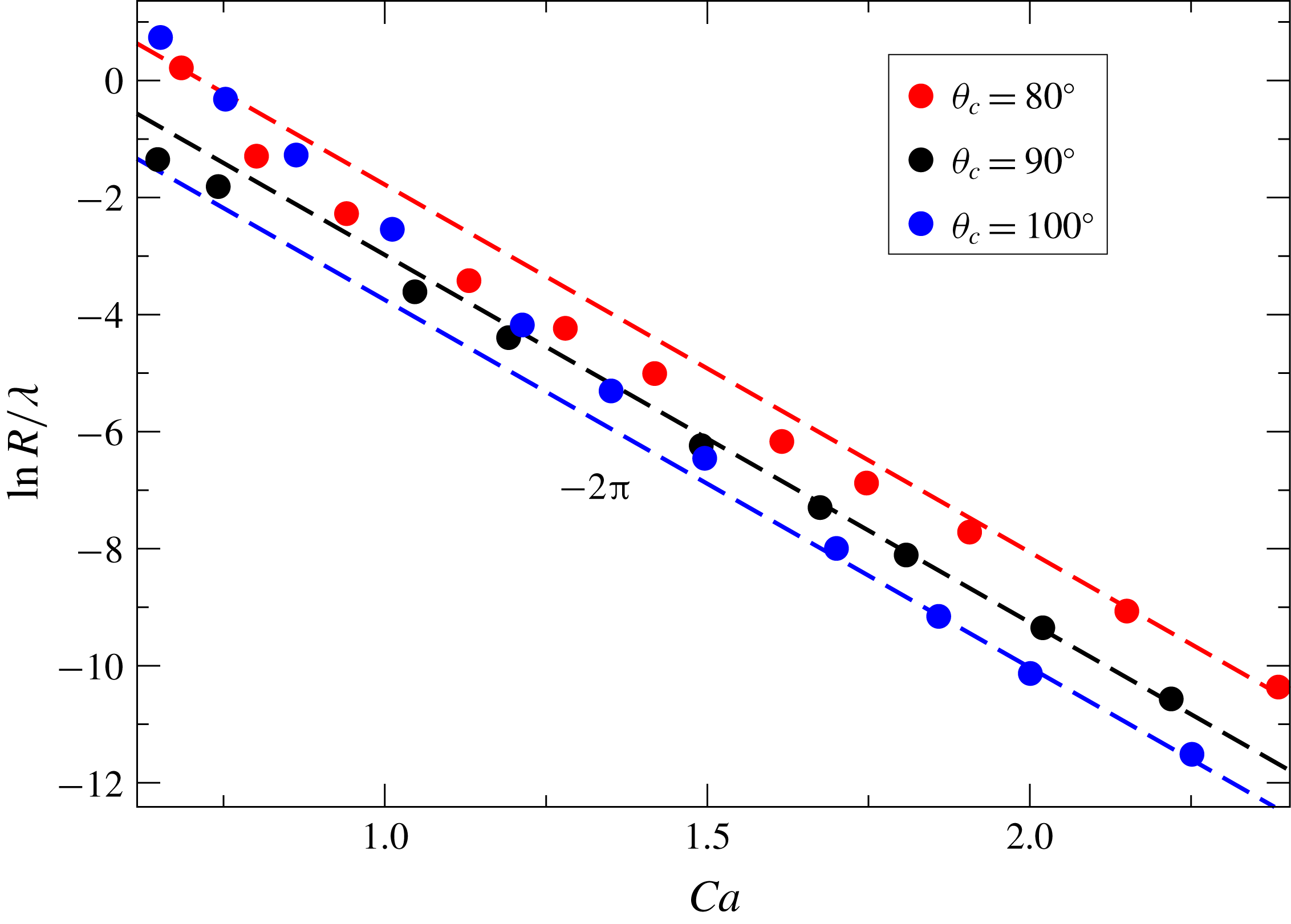
. Finally, figure 11 shows the dependence for different
 $\unicode[STIX]{x1D703}_{e}$
. We find that (2.18) is still valid, at least for high enough
 $Ca$
. This confirms our earlier conclusion that the form of the cusp region is independent of
 $\unicode[STIX]{x1D703}_{e}$
; however, the value of
 $C$
depends significantly on
 $\unicode[STIX]{x1D703}_{e}$
.


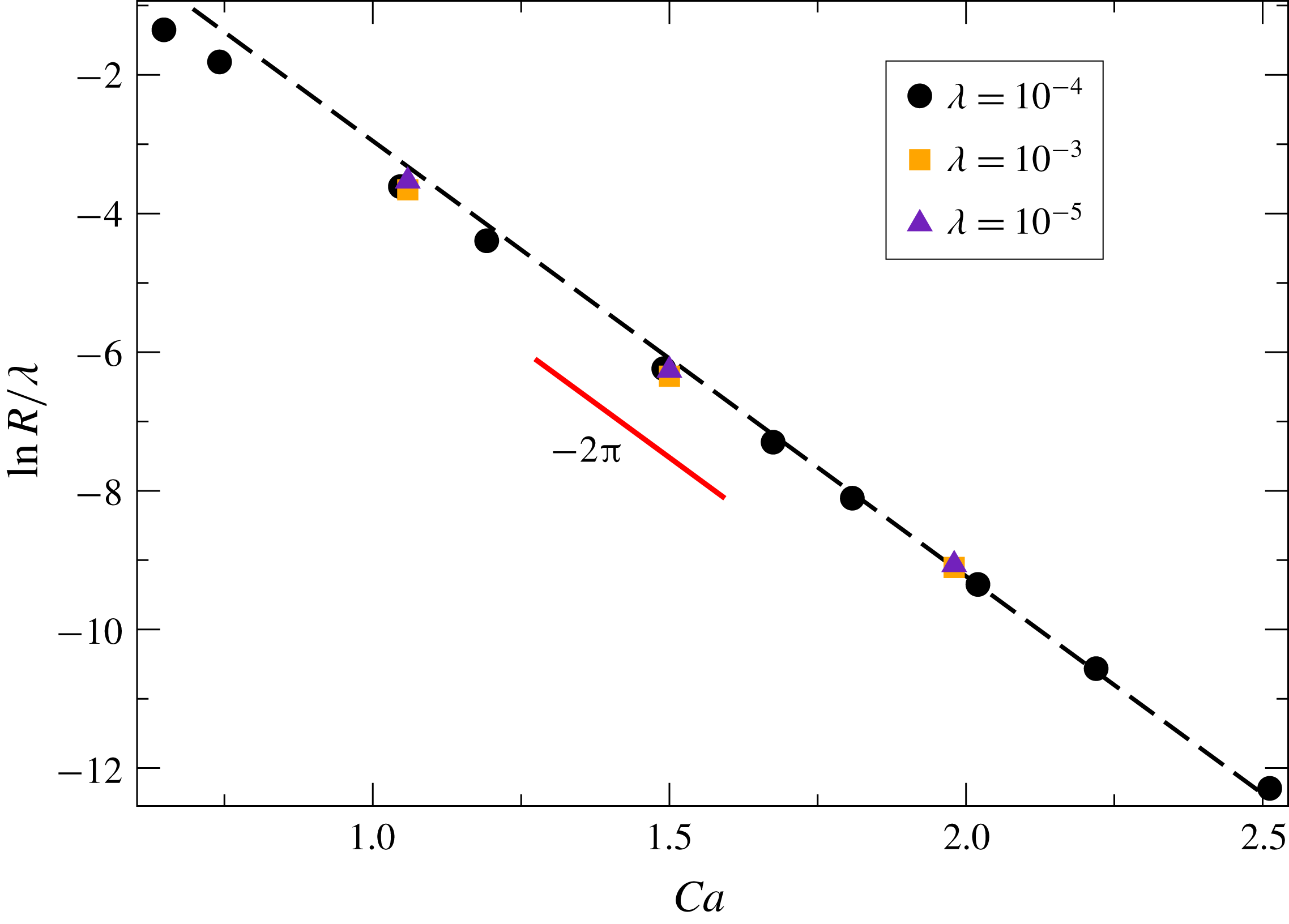
Plot of
 $R/\unicode[STIX]{x1D706}$
for different
 $\unicode[STIX]{x1D703}_{e}$
. The radius
 $R$
is found by fitting (2.13) to FEM simulations, just like for
 $\unicode[STIX]{x1D703}_{e}=90^{\circ }$
. As
 $Ca$
increases, all curves eventually collapse onto a line with exponent
 $-2\unicode[STIX]{x03C0}$
. The value of
 $C$
in (2.18) is
 $C=3.22$
for
 $\unicode[STIX]{x1D703}_{e}=80^{\circ }$
,
 $C=4.29$
for
 $\unicode[STIX]{x1D703}_{e}=90^{\circ }$
and
 $C=146$
for
 $\unicode[STIX]{x1D703}_{e}=100^{\circ }$
.
2.3 Region III: the bath
To complete the description of the profile for
 $M=0$
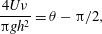
, we consider how the profile levels off towards a flat bath. The flow far from the interface should be well described by a flow in a rectangular corner, driven by the moving vertical plate. The other side of the corner is formed by the free surface. This amounts to using the GL approximation (see appendix A) in the limit
 $\unicode[STIX]{x1D703}\rightarrow \unicode[STIX]{x03C0}/2$
, for which
 $F\approx -4/(3\unicode[STIX]{x03C0})$
, as found from (A 2). Surface tension is subdominant on a scale much larger than
 $l_{c}$
, as we will confirm self-consistently; of course, we can set
 $\unicode[STIX]{x1D706}=0$
as well. Thus from (A 1) we obtain to leading order in
 $\unicode[STIX]{x1D703}-\unicode[STIX]{x03C0}/2$
in dimensional variables
 $$\begin{eqnarray}\displaystyle \frac{4U\unicode[STIX]{x1D708}}{\unicode[STIX]{x03C0}gh^{2}}=\unicode[STIX]{x1D703}-\unicode[STIX]{x03C0}/2, & & \displaystyle\end{eqnarray}$$
where
 $\unicode[STIX]{x1D708}=\unicode[STIX]{x1D702}/\unicode[STIX]{x1D70C}$
. From (A 4) we obtain to leading order
 $$\begin{eqnarray}\displaystyle \frac{\text{d}h}{\text{d}x}=\frac{1}{\unicode[STIX]{x1D703}-\unicode[STIX]{x03C0}/2}, & & \displaystyle\end{eqnarray}$$
so that
 $$\begin{eqnarray}\displaystyle \frac{4U\unicode[STIX]{x1D708}}{\unicode[STIX]{x03C0}g}\frac{\text{d}h}{h^{2}}=\text{d}x. & & \displaystyle\end{eqnarray}$$
Integrating, we find
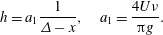 $$\begin{eqnarray}\displaystyle h=a_{1}\frac{1}{\unicode[STIX]{x1D6E5}-x},\quad a_{1}=\frac{4U\unicode[STIX]{x1D708}}{\unicode[STIX]{x03C0}g}. & & \displaystyle\end{eqnarray}$$
This agrees well with numerical simulations for
 $H_{b}=10^{3}$
(dimensionally a domain width
 $1000$
times the capillary length); as shown in the inset in figure 12, data points approach the theoretical prediction for large
 $Ca$
.
FEM simulations of the interface about the bath for
 $Ca=0.75$
, 1.04 and 1.49 (bottom to top) for
 $H_{b}=10^{3}$
(black lines). The short (red) line in the main panel represents the power law
 $h\sim (\unicode[STIX]{x1D6E5}-x)^{-1}$
. In the inset we show the coefficient of proportionality
 $a_{1}$
as found by fitting FEM simulations to
 $h=a_{1}(\unicode[STIX]{x1D6E5}-x)^{-1}$
and compare to the theoretical prediction (2.22) (red line).

3 The drying transition
We have found that, for high capillary numbers, the structure of the solution in the absence of a gas atmosphere is very similar to the free-surface cusps found on the surface of a viscous liquid in the absence of a solid (Jeong & Moffatt Reference Jeong and Moffatt1992; Eggers & Fontelos Reference Eggers and Fontelos2013). To describe the bifurcation towards a state where gas is entrained, we can therefore use the theory developed for free-surface cusps (Eggers Reference Eggers2001), which has been confirmed experimentally (Lorenceau, Restagno & Quéré Reference Lorenceau, Restagno and Quéré2003; Kiger & Duncan Reference Kiger and Duncan2012).
The idea is that the air being dragged into the narrow cusp produces a lubrication pressure, which forces the two sides apart. Making use of the slenderness of the cusp, we calculate the extra velocity generated by the gas forcing. The condition for a steady profile leads to an integral equation for the perturbed profile, which has a saddle-node bifurcation with a stable upper branch and an unstable lower branch, as in figure 3. A key point is that the perturbation to the
 $M=0$
profile necessary to create a bifurcation is very small, so that a quantitative description can be obtained by adding the velocity generated by the gas as a perturbation.
We begin by testing this theoretical description using the full numerical profiles for
 $M=0$
, adding the perturbation coming from the gas, finding good quantitative agreement with the theoretical bifurcation curves. Then we present an approximate description based on the theoretical approximation (2.13) for the cusp. At the same time we use an approximate method to solve the integral equation, which still reproduces all the essential features of the original solution, while giving analytical insight into the bifurcation.
3.1 The bifurcation
We solve the gas flow in the narrow space between the liquid and solid for a given
 $M=0$
solution. Since the geometry is slender, we can use lubrication theory (Eggers & Fontelos Reference Eggers and Fontelos2015) to calculate the pressure inside the gap. As usual in lubrication theory, the pressure is constant over a cross-section of the gap, and the normal stress the gas exerts on the fluid is dominated by the pressure. The shear stress is subdominant in lubrication theory. If
 $u_{0}(x)$
is the vertical velocity of the fluid on the interface, the vertical velocity in the gap, using a quadratic approximation, is
 $$\begin{eqnarray}\displaystyle u_{g}(x,y)=a_{2}y^{2}+a_{1}y+a_{1}\unicode[STIX]{x1D706}_{g}-U,\quad a_{2}=\frac{p_{x}}{2M\unicode[STIX]{x1D702}},\quad a_{1}=\frac{u_{0}+U-a_{2}h^{2}}{h+\unicode[STIX]{x1D706}_{g}}. & & \displaystyle\end{eqnarray}$$
It is easily verified that, for
 $y=h(x)$
, the velocity is continuous, while for
 $y=0$
(on the plate), the partial-slip condition (1.6) (third equation) is satisfied. From the condition that the total flux
 $\int _{0}^{h}u_{g}\,\text{d}y$
through the gap must vanish, we obtain
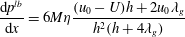 $$\begin{eqnarray}\displaystyle \frac{\text{d}p^{lb}}{\text{d}x}=6M\unicode[STIX]{x1D702}\frac{(u_{0}-U)h+2u_{0}\unicode[STIX]{x1D706}_{g}}{h^{2}(h+4\unicode[STIX]{x1D706}_{g})} & & \displaystyle\end{eqnarray}$$
for the derivative of the lubrication pressure with respect to
 $x$
. To obtain the pressure, one can integrate (3.2) starting from the bath, where the pressure is that of the ambient gas. The lubrication pressure increases rapidly as the gap becomes narrower, which is the root cause of the bifurcation. The growth of the pressure is mitigated somewhat by the presence of the slip
 $\unicode[STIX]{x1D706}_{g}$
. The liquid flow is calculated for
 $M=0$
, which supplies
 $u_{0}$
, from which the lubrication pressure is calculated via (3.2). This produces a correction to the stress balance on the free surface, which changes the liquid flow, so both liquid and gas flow have to be calculated self-consistently. A scheme of calculating the effect of the gas by lubrication theory was implemented numerically by Liu et al. (Reference Liu, Vandre, Carvalho and Kumar2016) and Sprittles (Reference Sprittles2017). In both papers it is confirmed that, at least when the capillary number is sufficiently high, results based on the lubrication approximation in the gas are almost indistinguishable from numerical simulations where both phases are treated equally.
However, this approach still requires a full numerical simulation of the liquid phase for each value of
 $M$
. In order to capture the effect of the gas analytically, as in Eggers (Reference Eggers2001) we observe that the cusp is similar to a crack in an infinite two-dimensional fluid domain, with a normal load imposed on it. Exploiting the equivalence between linear elasticity and the Stokes equation in two dimensions, one can use classical results from elasticity (Sun Reference Sun2011) to compute the extra velocity
 $v_{M}(x)$
coming from the stress on the cusp surface:
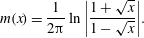
 $$\begin{eqnarray}\displaystyle v_{M}(x)=\frac{1}{\unicode[STIX]{x1D702}}\int _{0}^{\unicode[STIX]{x1D6E5}}p^{lb}(x^{\prime })m(x^{\prime }/x)\,\text{d}x^{\prime }, & & \displaystyle\end{eqnarray}$$
where
 $$\begin{eqnarray}\displaystyle m(x)=\frac{1}{2\unicode[STIX]{x03C0}}\ln \left|\frac{1+\sqrt{x}}{1-\sqrt{x}}\right|. & & \displaystyle\end{eqnarray}$$
The upper limit
 $\unicode[STIX]{x1D6E5}$
represents the undisturbed bath, where the ambient pressure has been reached. Note the crucial feature that
 $v_{M}$
is a non-local function of the load
 $p^{lb}$
, while in the GL approximation, where (3.2) enters into (A 1) through
 $F(\unicode[STIX]{x1D703},M)$
, the interface description is affected by
 $p^{lb}$
only locally.
Integrating (3.3) by parts gives
 $$\begin{eqnarray}\displaystyle v_{M}(x)=-\frac{x}{\unicode[STIX]{x1D702}}\int _{0}^{\unicode[STIX]{x1D6E5}}p_{x}^{lb}(x^{\prime }){\mathcal{M}}(x^{\prime }/x)\,\text{d}x^{\prime }, & & \displaystyle\end{eqnarray}$$
where
 $$\begin{eqnarray}\displaystyle {\mathcal{M}}(x)=\int _{0}^{x}m(x^{\prime })\,\text{d}x^{\prime }=\frac{1}{\unicode[STIX]{x03C0}}\left[\sqrt{x}+\frac{x-1}{2}\ln \left|\frac{1+\sqrt{x}}{1-\sqrt{x}}\right|\right]. & & \displaystyle\end{eqnarray}$$
The requirement that the free surface be a streamline of the flow is
 $$\begin{eqnarray}\displaystyle \frac{\unicode[STIX]{x2202}h}{\unicode[STIX]{x2202}x}=\frac{v(x)}{u(x)}\approx \frac{v_{0}(x)+v_{M}(x)}{u_{0}(x)}=\frac{\unicode[STIX]{x2202}h_{0}}{\unicode[STIX]{x2202}x}+\frac{\unicode[STIX]{x2202}h^{c}}{\unicode[STIX]{x2202}x},\quad h=h_{0}+h^{c}(x), & & \displaystyle\end{eqnarray}$$
where we have assumed that
 $v_{M}$
can be added to the base flow in a perturbative fashion, as explained before. Here
 $h_{0}(x)$
represents the initial
 $M=0$
base profile, and
 $h^{c}(x)$
the perturbation from this base profile for a given
 $M$
. Since
 $v_{0}$
and
 $v_{M}$
have opposite signs, the effect of the air is to push the interface so as to make it steeper, effectively narrowing the gap, decreasing
 $h$
. According to (3.2), the pressure rapidly increases with decreasing
 $h$
, amplifying the effect of the air. This positive feedback leads to a bifurcation at a critical value of the capillary number.
As described in the introduction and seen in figure 3, to find both stable and unstable branches of the bifurcation curve, one fixes the depression
 $\unicode[STIX]{x1D6E5}$
, and searches for the corresponding value of
 $Ca$
. However, since the base profile, which is available to us numerically only, depends on
 $Ca$
but is by definition independent of
 $M$
, it is more convenient to fix
 $\unicode[STIX]{x1D6E5}$
as well as
 $Ca$
and search for
 $M$
, as seen in figure 13. Once the critical value of
 $M$
has been found for different values of
 $Ca$
, one can produce the conventional plot of
 $Ca_{cr}$
as a function of
 $M$
(cf. figure 14).
Equations (3.5) and (3.7) are solved numerically for
 $h^{c}(x)$
. The unperturbed profile
 $h_{0}$
, as well as the base solution
 $u_{0}(x)$
and
 $v_{0}(x)$
for the velocity field, evaluated at the free surface, are taken from the numerical simulation for
 $M=0$
. Starting from
 $\unicode[STIX]{x1D6E5}(M=0)$
, the depression is increased slowly, and the value of
 $M$
is sought, using the previous solution as an initial condition. At each new value of
 $\unicode[STIX]{x1D6E5}$
, the profile
 $h(x)$
is discretized, and (3.7) is solved using Newton’s method. Since the changes in both the profile and
 $M$
from the preceding step are very small, only a few iterations are needed for both the new profile and value of
 $M$
to converge to high accuracy. The process is repeated and the value of
 $M(\unicode[STIX]{x0394})$
recorded. Successive iterations result in a bifurcation curve as shown in figure 13 as the solid black line, for
 $Ca=0.65$
and
 $Ca=1.04$
. Thus, to compare how the perturbation
 $\unicode[STIX]{x0394}(M)$
and
 $h_{M}^{c}(x)$
increases compared to the numerical simulations, we first compare bifurcation plots perturbing from the same
 $M=0$
solution, found from the FEM simulations. This is shown in figure 13.
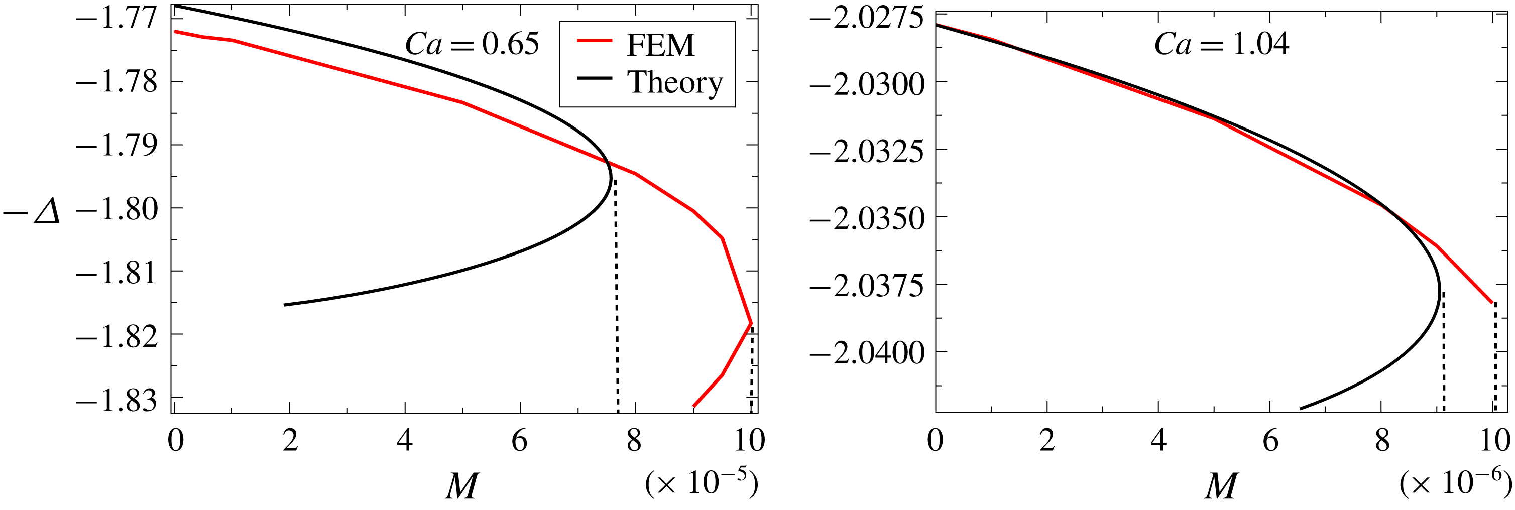
Bifurcation curve obtained from theory, using the base flow obtained from numerical simulation at
 $M=0$
for
 $Ca=0.65$
and
 $Ca=1.04$
(solid black line), compared to full FEM simulations (red line). The contact angle is
 $\unicode[STIX]{x1D703}_{e}=\unicode[STIX]{x03C0}/2$
and slip lengths are
 $\unicode[STIX]{x1D706}_{l}=\unicode[STIX]{x1D706}_{g}=10^{-4}$
. Vertical dashed lines mark the critical values
 $M_{cr}$
.
The critical capillary number
 $Ca_{cr}$
as a function of
 $M$
according to FEM data (red squares) and theory (blue circles), for
 $\unicode[STIX]{x1D706}=\unicode[STIX]{x1D706}_{g}=10^{-4}$
and
 $\unicode[STIX]{x1D703}_{e}=\unicode[STIX]{x03C0}/2$
. The solid line corresponds to the analytical prediction according to (3.14), and the dashed line is the analytical prediction including slip between gas and the liquid; the vertical dotted line denotes the theoretical limit (3.19) below which no bifurcation occurs.

The plots for
 $M(\unicode[STIX]{x1D6E5})$
in figure 13 show a saddle-node bifurcation: there is a critical
 $M_{cr}$
at which the upper branch from this point is stable and the lower branch is unstable. This bifurcation point corresponds to the point where a dynamic drying transition would occur as the value of
 $M$
is raised. The lower branch is unstable. The red line corresponds to the result of the FEM simulation; it was obtained by extrapolating the bifurcation curve
 $Ca(\unicode[STIX]{x1D6E5})$
obtained numerically for a range of
 $M$
values to a curve
 $M(\unicode[STIX]{x1D6E5})$
at fixed
 $Ca$
. It is seen that, for the larger value of
 $Ca$
(
 $Ca=1.04$
), the agreement is almost perfect along the upper branch, and the extrapolated value of
 $M$
where the bifurcation occurs is very close to the bifurcation point predicted by theory. However, owing to computational issues, previously described, we were not able to capture the lower branch in numerical simulations. We estimate the bifurcation point from a sudden increase of the curvature of the bifurcation curve. Trying to extrapolate our data beyond the bifurcation point, we estimate that our critical values of
 $M$
might be too low by as much as 10 %. For the smaller
 $Ca$
(
 $Ca=0.65$
), a lower branch is seen in both the numerical simulation and theory. The price we have to pay is that our asymptotic description is not quite as good, and the value of the critical
 $M$
is overestimated by approximately
 $20\,\%$
. Still, the bifurcation curve is predicted convincingly, without adjustable parameters. The comparison between FEM results and theory is summarized in figure 14 for an angle of
 $\unicode[STIX]{x1D703}_{e}=\unicode[STIX]{x03C0}/2$
and slip lengths
 $\unicode[STIX]{x1D706}=\unicode[STIX]{x1D706}_{g}=10^{-4}$
. The FEM data are the same as given in figure 2, with slip lengths chosen to match the simulations of Vandre et al. (Reference Vandre, Carvalho and Kumar2013). As shown in Sprittles (Reference Sprittles2017), the experimental results of figure 2 are well reproduced by numerical simulations, if appropriate physical slip lengths are chosen. Good agreement is found between our theory and simulations in figure 14 as long as
 $M$
values are sufficiently small for our asymptotic theory to be applicable. For small
 $M$
one observes a small rise of the critical capillary number over a generally logarithmic behaviour. This is because the presence of slip reduces the amount of air being dragged into the cusp region. To gain a better analytical understanding of these behaviours, we now present a simplified analytical theory of the transition.
3.2 Similarity description
We formulate (3.5) and (3.7) in terms of the phenomenological cusp solution (2.13). In order to be able to write the resulting equation in self-similar variables, we assume that the velocity
 $u_{0}=-U$
along the cusp is constant. If (2.14) represents the base solution for
 $M=0$
, the full solution reads in similarity variables:
 $$\begin{eqnarray}\displaystyle h=R^{q/(2q-1)}H(\unicode[STIX]{x1D709}),\quad \unicode[STIX]{x1D709}=R^{1/(1-2q)}x,\quad H(\unicode[STIX]{x1D709})=H_{0}(\unicode[STIX]{x1D709})+H^{c}(\unicode[STIX]{x1D709}), & & \displaystyle\end{eqnarray}$$
where
 $H_{0}(\unicode[STIX]{x1D709})$
is the unperturbed (
 $M=0$
) similarity solution described by (2.14), and
 $H^{c}(\unicode[STIX]{x1D709})$
is the correction coming from the effect of air in the narrow gap. Using
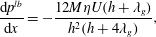
 $u_{0}=-U$
, we have
 $$\begin{eqnarray}\displaystyle \frac{\text{d}p^{lb}}{\text{d}x}=-\frac{12M\unicode[STIX]{x1D702}U(h+\unicode[STIX]{x1D706}_{g})}{h^{2}(h+4\unicode[STIX]{x1D706}_{g})}, & & \displaystyle\end{eqnarray}$$
so using (3.7) and (3.6), the equation for
 $H^{c}(\unicode[STIX]{x1D709})$
becomes
 $$\begin{eqnarray}\displaystyle \frac{\text{d}H^{c}}{\text{d}\unicode[STIX]{x1D709}}=-12s\unicode[STIX]{x1D709}\int _{0}^{\infty }\frac{{\mathcal{M}}(\unicode[STIX]{x1D70F}/\unicode[STIX]{x1D709})(H(\unicode[STIX]{x1D70F})+\bar{\unicode[STIX]{x1D706}}_{g})\,\text{d}\unicode[STIX]{x1D70F}}{H^{2}(\unicode[STIX]{x1D70F})(H(\unicode[STIX]{x1D70F})+4\bar{\unicode[STIX]{x1D706}}_{g})}, & & \displaystyle\end{eqnarray}$$
where
 $$\begin{eqnarray}\displaystyle s=MR^{3(q-1)/(1-2q)},\quad \bar{\unicode[STIX]{x1D706}}_{g}=R^{q/(1-2q)}\unicode[STIX]{x1D706}_{g}. & & \displaystyle\end{eqnarray}$$
Together with (3.8), this is an equation for the perturbation
 $H^{c}(\unicode[STIX]{x1D709})$
. From the behaviour of the kernel,
 $$\begin{eqnarray}\displaystyle \lim _{x\rightarrow 0}{\mathcal{M}}(x)=\frac{2x^{3/2}}{3\unicode[STIX]{x03C0}},\quad \lim _{x\rightarrow \infty }{\mathcal{M}}(x)=\frac{2\sqrt{x}}{\unicode[STIX]{x03C0}}, & & \displaystyle\end{eqnarray}$$
one can deduce that
 $(\text{d}H^{c}/\text{d}\unicode[STIX]{x1D709})\unicode[STIX]{x1D709}^{1/2}$
for
 $\unicode[STIX]{x1D709}\rightarrow 0$
and
 $\text{d}H^{c}/\text{d}\unicode[STIX]{x1D709}\propto \,\unicode[STIX]{x1D709}^{-1/2}$
for
 $\unicode[STIX]{x1D709}\rightarrow \infty$
. It follows that
 $H_{c}(\unicode[STIX]{x1D709})$
behaves asymptotically as
 $$\begin{eqnarray}\displaystyle \lim _{\unicode[STIX]{x1D709}\rightarrow 0}H^{c}(\unicode[STIX]{x1D709})=-H_{0}\unicode[STIX]{x1D709}^{3/2},\quad \lim _{\unicode[STIX]{x1D709}\rightarrow \infty }H^{c}(\unicode[STIX]{x1D709})=-H_{i}\unicode[STIX]{x1D709}^{1/2}, & & \displaystyle\end{eqnarray}$$
where
 $H_{0}$
and
 $H_{i}$
are constants, which need to be found as part of the solution of (3.10). In particular, the integral in (3.10) is convergent at both the lower and upper boundary, so non-universal effects having to do with either the bath or the contact line region do not play a role asymptotically.
Now we solve (3.10) numerically for a given capillary number, putting
 $H(\unicode[STIX]{x1D709})=\sqrt{2\unicode[STIX]{x1D709}}+a\unicode[STIX]{x1D709}^{q}+H^{c}(\unicode[STIX]{x1D709})$
. This is essentially the same equation as that solved numerically in Eggers (Reference Eggers2001) using Newton’s method. We find a saddle-node bifurcation at a critical value
 $s=s_{c}$
, above which there is no more solution, while below
 $s_{c}$
there are two branches, one stable and one unstable. To identify both branches, we treat
 $s$
as an unknown in (3.10), holding
 $H_{i}$
(cf. (3.13)) constant. Clearly, the larger values of
 $H_{i}$
correspond to the unstable branch, the smaller values to the stable branch; solving (3.10), we find
 $s$
for each value of
 $H_{i}$
. The maximum of the curve
 $s(H_{i})$
corresponds to
 $s_{c}$
.
With
 $s_{c}(q,a,\bar{\unicode[STIX]{x1D706}}_{g})$
in hand, we are able to make a theoretical prediction for the critical capillary number shown in figure 14, without using a FEM simulation of the
 $M=0$
solution. The dependence of the radius of curvature on
 $Ca$
is given by (2.18), and so the first equation of (3.11) yields
 $$\begin{eqnarray}\displaystyle M=s_{c}(q,a,\bar{\unicode[STIX]{x1D706}}_{g})(\text{e}^{2+\unicode[STIX]{x1D6FE}_{E}}C\unicode[STIX]{x1D706})^{3(1-q)/(1-2q)}\exp \left(-\frac{6\unicode[STIX]{x03C0}(q-1)}{2q-1}Ca_{cr}\right). & & \displaystyle\end{eqnarray}$$
This is the inverse of
 $Ca_{cr}(M)$
, and is shown as the solid line in figure 14. We have used
 $C=4.29$
(cf. figure 10),
 $q$
as calculated from (2.10), and
 $a$
using the fit from figure 8. The rescaled slip length
 $\bar{\unicode[STIX]{x1D706}}_{g}$
in the gas is found from (3.11). The expression (3.14) combines all theoretical results from this paper, providing a unified asymptotic description of the critical capillary number in terms of all relevant parameters.
The solid line agrees well with both full FEM simulations (red squares) and the abridged theory based on knowledge of the full solution for
 $M=0$
(blue circles), as long as
 $Ca_{cr}$
is sufficiently high, meaning that
 $M$
is smaller than approximately
 $10^{-4}$
. For moderate values of
 $M$
, meaning that
 $Ca$
is small, the rescaled slip length
 $\bar{\unicode[STIX]{x1D706}}_{g}$
is small and can effectively be put to zero. Thus, apart from the weak dependence of
 $q$
and
 $a$
on
 $Ca$
,
 $s_{c}$
is a constant, and solving (3.14) for
 $Ca_{cr}$
leads to the logarithmic behaviour
 $$\begin{eqnarray}\displaystyle Ca_{cr}=\frac{2q-1}{6\unicode[STIX]{x03C0}(1-q)}\ln \frac{M}{s_{c}}+\frac{2+\unicode[STIX]{x1D6FE}_{E}+\ln (C\unicode[STIX]{x1D706})}{2\unicode[STIX]{x03C0}}, & & \displaystyle\end{eqnarray}$$
which is seen in figure 14 for
 $M\lesssim 10^{-4}$
. For smaller values of
 $M$
, on the other hand,
 $Ca_{cr}$
becomes somewhat larger than predicted by this logarithmic law. The reason is that slip between the gas and the solid wall regularizes the growth of the lubrication pressure, so higher speeds are needed to trigger the bifurcation. However, as seen from (3.10), even in the limit of
 $\bar{\unicode[STIX]{x1D706}}_{g}\rightarrow \infty$
, the gradient is reduced by a factor of
 $1/2$
only, compared to
 $\bar{\unicode[STIX]{x1D706}}_{g}=0$
.
The reason for the insensitivity to
 $\unicode[STIX]{x1D706}_{g}$
is that we still do not allow slip between the gas and the liquid, so that the gas is still dragged into the gap by the liquid’s motion, with the channel effectively twice as wide, as the gas does not encounter any resistance at the wall. If one were to treat the gas flow near the interface with the same slip law as with the wall, as suggested by kinetic effects (Li Reference Li2016; Sprittles Reference Sprittles2017), (3.10) would turn into
 $$\begin{eqnarray}\displaystyle \frac{\text{d}H^{c}}{\text{d}\unicode[STIX]{x1D709}}=-12s\unicode[STIX]{x1D709}\int _{0}^{\infty }\frac{{\mathcal{M}}(\unicode[STIX]{x1D70F}/\unicode[STIX]{x1D709})\,\text{d}\unicode[STIX]{x1D70F}}{H(\unicode[STIX]{x1D70F})(H(\unicode[STIX]{x1D70F})+6\bar{\unicode[STIX]{x1D706}}_{g})}. & & \displaystyle\end{eqnarray}$$
Clearly, the effect of the gas on the right-hand side now becomes small for large
 $\bar{\unicode[STIX]{x1D706}}$
, i.e. for small
 $R$
. Instead of the solid line in figure 14, we now obtain the dashed line, which rises rapidly at
 $M\approx 10^{-6}$
, leading to a sharp deviation from the weak logarithmic dependence usually associated with the drying transition.
To make this observation more quantitative, we consider the asymptotic limit of
 $\bar{\unicode[STIX]{x1D706}}_{g}$
very large in (3.16), so that
 $H(\unicode[STIX]{x1D70F})$
can be neglected in comparison. As a result, we obtain
 $$\begin{eqnarray}\displaystyle \frac{\text{d}H^{c}}{\text{d}\unicode[STIX]{x1D709}}=-2\bar{s}\unicode[STIX]{x1D709}\int _{0}^{\infty }\frac{{\mathcal{M}}(\unicode[STIX]{x1D70F}/\unicode[STIX]{x1D709})\,\text{d}\unicode[STIX]{x1D70F}}{H(\unicode[STIX]{x1D70F})}, & & \displaystyle\end{eqnarray}$$
where we have introduced
 $\bar{s}=s/\bar{\unicode[STIX]{x1D706}}_{g}$
. For large
 $Ca$
, the cusp exponent (2.10) becomes
 $q=3/2$
, so the only remaining parameter in (3.17) is
 $a$
; we take it to be its asymptotic value
 $a=0.45$
. Solving the integral equation (3.17) as before, we obtain a critical value
 $\bar{s}_{c}=0.0272$
above which no solution exists. Combining the definition of
 $\bar{s}_{c}$
with (3.11), we obtain
 $$\begin{eqnarray}\displaystyle M=\bar{s}_{c}\unicode[STIX]{x1D706}_{g}R^{(3-2q)/(1-2q)}. & & \displaystyle\end{eqnarray}$$
Note that, for the asymptotic value
 $q=3/2$
, the exponent vanishes, so we have to include the next order
 $q=3/2+1/(2\unicode[STIX]{x03C0}Ca)$
to obtain
 $1/(2\unicode[STIX]{x03C0}Ca)$
for the exponent in (3.18) to leading order as
 $Ca\rightarrow \infty$
. Together with the formula (2.18) for
 $R$
, this yields, to leading order as
 $Ca\rightarrow \infty$
, that the right-hand side of (3.18) reaches a finite value in the limit. This means there exists a critical value
 $$\begin{eqnarray}\displaystyle M_{c}=0.0272\unicode[STIX]{x1D706}_{g}/e & & \displaystyle\end{eqnarray}$$
of
 $M$
below which no bifurcation occurs, regardless of how large the capillary number is. For the parameters of figure 14, this is
 $\log _{10}M_{c}=-6$
(shown as the dotted vertical line), in good agreement with the sharp rise of the dashed line at that point.
4 Discussion
In this paper, we present a theory of air entrainment which takes account of the fact that critical capillary numbers are not small, so an expansion in the capillary number fails. First we develop an asymptotic description of the interface for large capillary numbers, for which the interface forms a cusp, described by (2.14). The radius of curvature
 $R$
at the contact line scales like the slip length, multiplied by an exponential of the capillary number. As a result, the typical scale of the solution near the contact line, below which wetting properties come into play, may be much smaller than the slip length. In a second step we take into account the air by calculating the lubrication pressure inside the narrow cusp, which affects the flow in a non-local fashion. Changes in the no-slip boundary condition (for example, increasing the slip length) can delay the onset of the transition significantly.
By contrast, the conventional theory of the drying transition is based on an expansion for small capillary numbers (Voinov Reference Voinov1976; Cox Reference Cox1986), which yields for the angle
 $\unicode[STIX]{x1D703}_{d}$
at a distance
 $l_{d}$
from the contact line:
 $$\begin{eqnarray}\displaystyle g(\unicode[STIX]{x1D703}_{d},M)=g(\unicode[STIX]{x1D703}_{e},M)+\ln (l_{d}/\unicode[STIX]{x1D706})Ca. & & \displaystyle\end{eqnarray}$$
In the limit
 $M=0$
, the function
 $g(\unicode[STIX]{x1D703},M)$
is
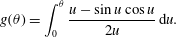 $$\begin{eqnarray}\displaystyle g(\unicode[STIX]{x1D703})=\int _{0}^{\unicode[STIX]{x1D703}}\frac{u-\sin u\cos u}{2u}\,\text{d}u. & & \displaystyle\end{eqnarray}$$
Cox (Reference Cox1986) proposed that a transition takes place when
 $\unicode[STIX]{x1D703}_{d}=\unicode[STIX]{x03C0}$
at some unspecified distance
 $l_{d}$
, although he himself acknowledged that the theory breaks down in this limit, even if
 $Ca$
is small. In (4.1) we have taken the inner length scale to be the slip length in the liquid, although the full picture may be more complicated; see appendix A. For small
 $M$
,
 $g(\unicode[STIX]{x03C0},M)\approx -(\unicode[STIX]{x03C0}/6)\ln (3\unicode[STIX]{x03C0}M/4)$
; assuming
 $\unicode[STIX]{x1D703}_{e}=\unicode[STIX]{x03C0}/2$
,
 $g(\unicode[STIX]{x03C0}/2,M)\approx g(\unicode[STIX]{x03C0}/2)=G-1/2$
, where
 $G\approx 0.915\ldots \,$
is Catalan’s constant. Thus the critical capillary number becomes
 $$\begin{eqnarray}\displaystyle Ca_{cr}=-\frac{\unicode[STIX]{x03C0}}{6\ln (l_{d}/\unicode[STIX]{x1D706})}\ln \frac{3\unicode[STIX]{x03C0}M}{4}-\frac{G-1/2}{\ln (l_{d}/\unicode[STIX]{x1D706})}. & & \displaystyle\end{eqnarray}$$
Assuming, somewhat arbitrarily, that
 $l_{d}$
is a constant independent of
 $Ca$
, (4.3) provides a prediction which contains a single adjustable constant. For example, fitting to the slope of the right-hand portion of figure 14 (which yields
 $\ln (l_{d}/\unicode[STIX]{x1D706})\approx 7.4$
), one obtains a reasonable description of the corresponding portion of the graph. However, the description (4.3) completely misses the upturn of the curve towards the left, for which slip in the gas phase is responsible. This is because the low-capillary-number theory is not able to account for the separate regularizing effect of gas slip in the narrow gap. Even more importantly, (4.1), on which Cox’s theory is based, fails to describe the concave shape of the cusp (2.13), as it has a concave shape, with the angle
 $\unicode[STIX]{x1D703}$
increasing monotonically. By contrast, in our theory, the slip in the gas phase enters in a way that is very different from the slip of the liquid. The latter sets the local scale for the size of the cusp tip, while the former regularizes the flow inside the cusp in a non-local fashion. In fact, it has been argued (Sprittles Reference Sprittles2017) that this regularizing effect is amplified even more if non-equilibrium effects are taken into account in the gas. It would be a straightforward addition to our theory to account for this when describing the gas flow in the gap.
Another important question is how (if at all) the wetting properties of the liquid (i.e. the equilibrium contact angle
 $\unicode[STIX]{x1D703}_{e}$
) come into play. In the low-capillary-number theory, wetting plays a crucial role, as (4.1) describes how the interface angle is bent away from its initial value at the contact line. On the other hand, there is recent experimental evidence (Eddi et al.
Reference Eddi, Winkels and Snoeijer2013; Latka et al.
Reference Latka, Boelens, Nagel and de Pablo2018) that wetting properties play no role for the spreading dynamics once the contact line speed is sufficiently high. As seen from (3.15), in the present theory the wetting angle comes in indirectly through the constant
 $C$
. According to the values reported in figure 11, there can thus be a variation of
 $Ca_{cr}$
by approximately 0.6 even in the narrow range
 $\unicode[STIX]{x1D703}_{e}=80^{\circ }{-}100^{\circ }$
. However, as shown in figure 9(b), the crossover towards the equilibrium contact angle takes place on a length scale that is much smaller than the slip length, which itself is of the order of the size of a few molecules. Thus the smallest length scale at an elevated capillary number may formally be smaller than a molecular scale. This suggests that it might in fact not be physically correct to resolve the flow to the smallest length scale produced by continuum theory. It remains an open question what the boundary condition should be, which correctly accounts for the presence of a molecular length scale.
Finally we mention that an interesting and important challenge would be to move beyond the two-dimensional theory developed here, to be able to describe the triangular air pockets which are often observed for
 $Ca=Ca_{cr}$
, as seen in figure 1(c). This problem has been looked at for the case of triangular liquid films formed when a solid plate is withdrawn from a bath (Snoeijer et al.
Reference Snoeijer, Le Grand, Limat, Stone and Eggers2007a
). In that case it was found that the entire three-dimensional flow in the film plays a role, rather than the inclination angle of the triangle being determined by a local argument alone.
Acknowledgements
J.E.S. acknowledges the support of the Leverhulme Trust (Research Project Grant) and the Engineering and Physical Sciences Research Council (grant nos EP/N016602/1, EP/P020887/1 and EP/P031684/1). J.E. acknowledges the support of the Leverhulme Trust International Academic Fellowship IAF-2017-010. We are grateful to T. S. Chan for providing us with figure 3.
Appendix A. The GL approximation for a
$90^{\circ }$
contact angle

The GL approximation for two-phase flow has been developed by Chan et al. (Reference Chan, Srivastava, Marchand, Andreotti, Biferale, Toschi and Snoeijer2013). The dependence of the model on the slip length is calculated phenomenologically by comparing to the result of lubrication theory at small contact angles
 $\unicode[STIX]{x1D703}_{e}$
. Here we are interested in contact angles closer to
 $\unicode[STIX]{x03C0}/2$
, needed to produce the data shown in figure 3. We report on the results of a recent investigation, details of which are to be published shortly (Chan et al.
Reference Chan, Eggers, Kamal and Snoeijer2018). To this end we start from the structure proposed by Chan et al. (Reference Chan, Srivastava, Marchand, Andreotti, Biferale, Toschi and Snoeijer2013), in which the effect of slip is accounted for by assuming the structure found for small angles:
 $$\begin{eqnarray}\displaystyle \frac{\text{d}^{2}\unicode[STIX]{x1D703}}{\text{d}s^{2}}=\frac{3Ca}{h(h+c\unicode[STIX]{x1D706})}F(\unicode[STIX]{x1D703},M)-\cos \unicode[STIX]{x1D703}. & & \displaystyle\end{eqnarray}$$
Here
 $\unicode[STIX]{x1D703}$
is the angle between the interface and the vertical (such that
 $\unicode[STIX]{x1D703}=\unicode[STIX]{x1D703}_{e}$
at the plate), and
 $s$
is the arclength of the interface from the contact line. The term on the left is the gradient of the Laplace pressure (since
 $\text{d}\unicode[STIX]{x1D703}/\text{d}s$
is the curvature), the first term on the right is the gradient of the pressure jump across the interface, as calculated from the Huh–Scriven solution (Huh & Scriven Reference Huh and Scriven1971), and the second term on the right comes from gravity. The function
 $F(\unicode[STIX]{x1D703},M)$
is given in Chan et al. (Reference Chan, Srivastava, Marchand, Andreotti, Biferale, Toschi and Snoeijer2013); to correct a small sign error, we report the result here:
 $$\begin{eqnarray}\displaystyle F=-\frac{2\sin ^{3}\unicode[STIX]{x1D703}}{3}\frac{M^{2}F_{1}(\unicode[STIX]{x1D703})+2MF_{3}(\unicode[STIX]{x1D703})+F_{1}(\unicode[STIX]{x03C0}-\unicode[STIX]{x1D703})}{MF_{1}(\unicode[STIX]{x1D703})F_{2}(\unicode[STIX]{x03C0}-\unicode[STIX]{x1D703})+F_{1}(\unicode[STIX]{x03C0}-\unicode[STIX]{x1D703})F_{2}(\unicode[STIX]{x1D703})}, & & \displaystyle\end{eqnarray}$$
where
 $$\begin{eqnarray}\displaystyle F_{1}=\unicode[STIX]{x1D703}^{2}-\sin ^{2}\unicode[STIX]{x1D703},\quad F_{2}=\unicode[STIX]{x1D703}-\sin \unicode[STIX]{x1D703}\cos \unicode[STIX]{x1D703},\quad F_{3}=\unicode[STIX]{x1D703}(\unicode[STIX]{x03C0}-\unicode[STIX]{x1D703})+\sin ^{2}\unicode[STIX]{x1D703}. & & \displaystyle\end{eqnarray}$$
The profile
 $h(x)$
is recovered from
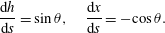 $$\begin{eqnarray}\displaystyle \frac{\text{d}h}{\text{d}s}=\sin \unicode[STIX]{x1D703},\quad \frac{\text{d}x}{\text{d}s}=-\text{cos}\,\unicode[STIX]{x1D703}. & & \displaystyle\end{eqnarray}$$
Integrating (A 1) in the absence of gravity one can show that for small
 $Ca$
the solution has the structure of the general form given by Cox (Reference Cox1986), but where the constant
 $c$
is unknown. Comparing (A 1) to lubrication theory with slip, one finds
 $c=3$
for small angles (Chan et al.
Reference Chan, Srivastava, Marchand, Andreotti, Biferale, Toschi and Snoeijer2013). To generalize this result to larger angles, we make use of the total shear force on the solid plate generated by a moving contact line with slip, which was calculated beyond the leading-order logarithmic behaviour by Hocking (Reference Hocking1977). Since the shear force must be balanced by the force supported by the interface, leading to the interface being curved, we can calculate the constant
 $c$
in terms of the shear force. The result (Chan et al.
Reference Chan, Eggers, Kamal and Snoeijer2018) is
 $$\begin{eqnarray}\displaystyle c=\sin \unicode[STIX]{x1D703}\exp \left(\frac{\sin \unicode[STIX]{x1D703}(h_{1}+Mh_{2})}{3F(\unicode[STIX]{x1D703},M)}\right), & & \displaystyle\end{eqnarray}$$
where, for
 $\unicode[STIX]{x1D703}_{e}=\unicode[STIX]{x03C0}/2$
,
 $$\begin{eqnarray}\displaystyle h_{1}=\frac{(1-M)h_{a}+2Mh_{b}}{1+M},\quad h_{2}=\frac{-(1-M)h_{a}+2Mh_{b}}{1+M}, & & \displaystyle\end{eqnarray}$$
and
 $h_{a}=(4/\unicode[STIX]{x03C0})(\unicode[STIX]{x1D6FE}-\ln 2)$
and
 $h_{b}=-1.539$
. In particular,
 $c\approx 1.12$
for
 $M=0$
, significantly smaller than the lubrication result
 $c=3$
. Equation (A 1) with
 $c$
as given in (A 5) was used to produce the results in figure 3.


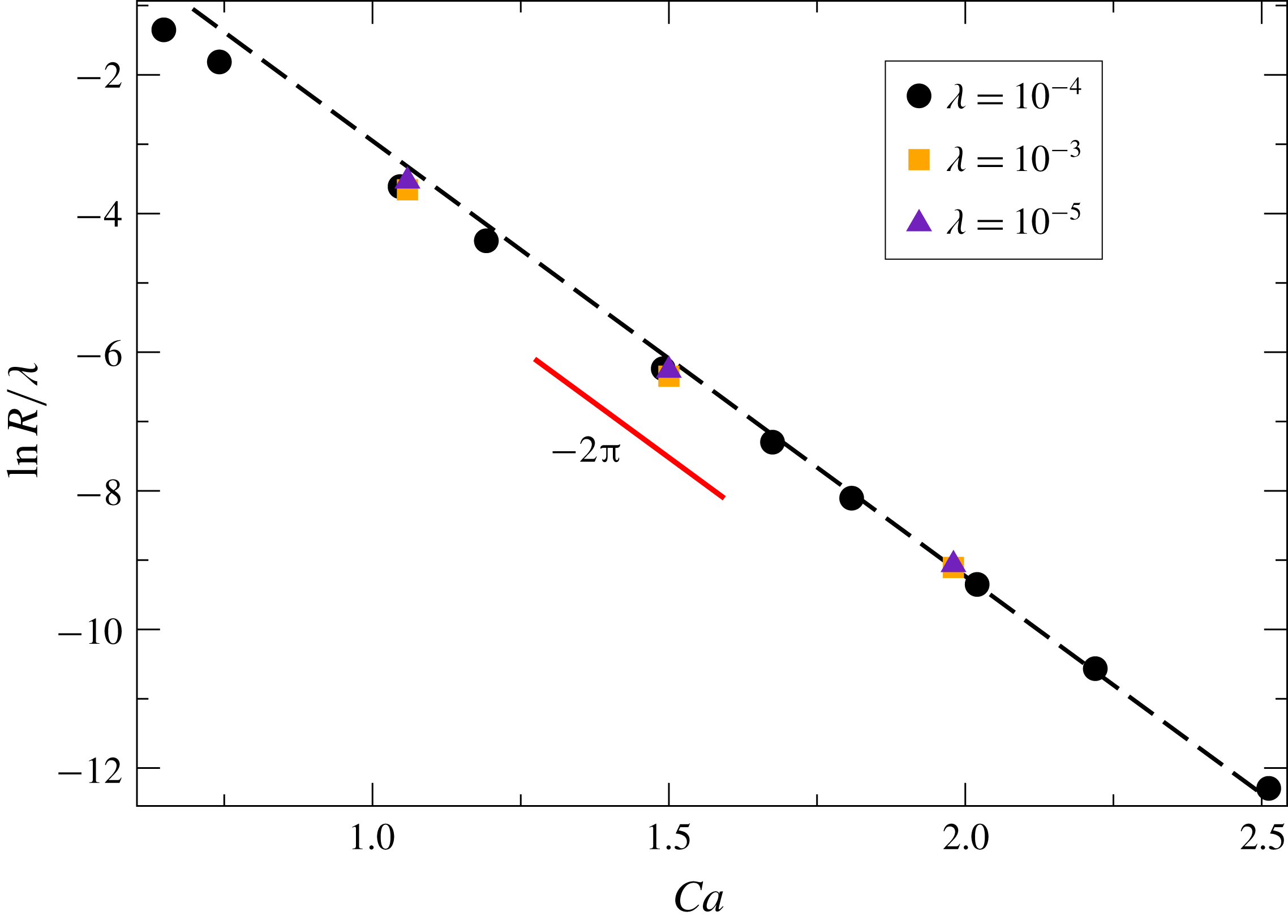


 Open access

