1 Introduction
The large-scale low-frequency variability (LFV) of the midlatitude ocean circulation on interannual to interdecadal time scales plays an important role in climate variability. Some of the LFV is either imposed by the atmosphere or is due to the ocean–atmosphere coupling, but this study focuses on the intrinsic, ocean-only LFV. Since the existence of the LFV was established observationally (Deser & Blackmon Reference Deser and Blackmon1993; Kushnir Reference Kushnir1994), many modelling studies have attempted to determine its patterns and mechanisms (McCalpin & Haidvogel Reference McCalpin and Haidvogel1996; Berloff & McWilliams Reference Berloff and McWilliams1999; Meacham Reference Meacham2000; Chang et al. Reference Chang, Ide, Ghil and Lai2001; Nauw & Dijkstra Reference Nauw and Dijkstra2001; Schmeits & Dijkstra Reference Schmeits and Dijkstra2002; Berloff, Hogg & Dewar Reference Berloff, Hogg and Dewar2007a ; Berloff et al. Reference Berloff, Kravtsov, Dewar and McWilliams2007b ; Kravtsov et al. Reference Kravtsov, Berloff, Dewar, Ghil and McWilliams2010; Simonnet Reference Simonnet2010; Feliks, Ghil & Robertson Reference Feliks, Ghil and Robertson2011; Pierini, Dijkstra & Mu Reference Pierini, Dijkstra and Mu2014; Kondrashov & Berloff Reference Kondrashov and Berloff2015). It is known now that collective action of oceanic mesoscale eddies is one of the main drivers of the midlatitude LFV (Kwon et al. Reference Kwon, Alexander, Bond, Frankignoul, Nakamura, Qiu and Thompson2010), which is generated in models only when a significant part of the mesoscale eddies is dynamically resolved. However, the computational cost of the eddy-resolving solutions is one of the main constraining factors that restricted most of the process studies to relatively viscous flow regimes characterized by transition to chaos rather than by developed turbulence. In contrast, patterns and mechanisms of the large-scale LFV revealed from the fully eddy-resolving, low-viscosity flow regimes still elude our understanding. Nevertheless, we already know that in eddy-permitting quasi-geostrophic (QG) models of ocean gyres, the robust LFV pattern is characterized by changes in the position and shape of the eastward jet and its adjacent recirculation zones (Berloff & McWilliams Reference Berloff and McWilliams1999). Berloff et al. (Reference Berloff, Hogg and Dewar2007a ) argue that this LFV is a fundamentally turbulent phenomenon driven by a dynamical competition between the eddy rectification process and the potential vorticity (PV) anomalies induced by changes of the intergyre PV transport. This LFV pattern and mechanism have been named the ‘turbulent oscillator’, and its stochastic statistical models were recently developed by Kondrashov & Berloff (Reference Kondrashov and Berloff2015). Analysis of similar LFV from a comprehensive ocean model is presently underway (Sérazin et al. Reference Sérazin, Penduff, Grégorio, Barnier, Molines and Terray2015). Despite the steady progress, the following important questions remain largely unanswered. What are the LFV patterns in highly turbulent flow regimes? To what extent can these patterns be deduced from the low-order bifurcations? What are the underlying physical mechanisms of the LFV? Can the LFV be simulated by simple reduced models?
In this work, we study the LFV in an eddy-resolving flow regime and propose a new approach for its dynamical interpretation. The key idea is to project the LFV, described here statistically by the leading empirical orthogonal functions (EOFs) and their principal components (PCs), onto the dynamically consistent eigenmodes obtained as solutions of the governing quasi-geostrophic equations linearized around the underlying time-mean circulation, and thus to develop a dynamical interpretation of the LFV. The novelty here is that, by using advanced computational technology, we are able to solve for spatially inhomogeneous eigenmodes of a general three-dimensional flow with a large number of degrees of freedom and to analyse and compare individual contributions of these modes to the LFV. The proposed approach can be extended to other idealized or comprehensive ocean models, as well as to more turbulent flow regimes.
2 Problem formulation
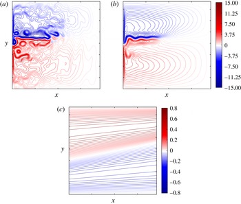
In this part we consider the classical double-gyre QG model, which describes idealized midlatitude ocean circulation and its linearization around the dynamically consistent time-mean background flow (figure 1 b) obtained from the reference eddy-resolving solution (figure 1 a). The explored flow regime was studied earlier by Shevchenko & Berloff (Reference Shevchenko and Berloff2015), who focused on the flow dependencies on the Reynolds number and other physical parameters.
Reference eddy-resolving double-gyre solution. Shown are (a) typical snapshot and (b) time-mean component of the transport velocity streamfunction
 ${\it\psi}_{1}$
(contour interval is 1.0 Sv), and (c) wind stress (contour interval is 0.05, arbitrary units). Note that most of the transient flow variability is concentrated around the eastward jet extension of the western boundary currents and its adjacent recirculation zones. Significant part of this variability is decadal and coherent on large scales.

2.1 Midlatitude ocean model
The three-layer QG equations (Pedlosky Reference Pedlosky1987; Vallis Reference Vallis2006) for the PV anomaly
 $q$
in a domain
 ${\it\Omega}$
are given by the PV material conservation law augmented with forcing and dissipation:
 $$\begin{eqnarray}\partial _{t}q_{j}+\text{J}({\it\psi}_{j},q_{j}+{\it\beta}y)={\it\delta}_{1j}F_{w}-{\it\delta}_{j3}{\it\mu}{\rm\Delta}{\it\psi}_{j}+{\it\nu}{\rm\Delta}^{2}{\it\psi}_{j},\quad j=1,2,3,\end{eqnarray}$$
where the Jacobian
 $\text{J}(f,g)\equiv f_{x}g_{y}-f_{y}g_{x}$
, and
 ${\it\delta}_{ij}$
is the Kronecker symbol; the computational domain
 ${\it\Omega}$
is a square, closed, flat-bottom basin of dimensions
 $L\times L\times H~\text{km}$
, with
 $L=3840~\text{km}$
, and
 $H=H_{1}+H_{2}+H_{3}$
is given by three stacked isopycnal fluid layers with depths (from top to bottom):
 $H_{1}=0.25~\text{km}$
,
 $H_{2}=0.75~\text{km}$
,
 $H_{3}=3.0~\text{km}$
.
The asymmetric wind curl forcing (figure 1 c), driving the double-gyre ocean circulation, is given by
 $$\begin{eqnarray}F_{w}=\left\{\begin{array}{@{}ll@{}}-1.80{\rm\pi}{\it\tau}_{0}\sin ({\rm\pi}y/y_{0}),\quad & y\in [0,y_{0}),\\ 2.22{\rm\pi}{\it\tau}_{0}\sin ({\rm\pi}(y-y_{0})/(L-y_{0})),\quad & y\in [y_{0},L],\end{array}\right.\end{eqnarray}$$
with the wind stress amplitude
 ${\it\tau}_{0}=0.3~\text{N}~\text{m}^{-2}$
and the tilted zero forcing line
 $y_{0}=0.4L+0.2x$
,
 $x\in [0,L]$
. The planetary vorticity gradient is
 ${\it\beta}=2\times 10^{-11}~\text{m}^{-1}~\text{s}^{-1}$
, the bottom friction parameter is
 ${\it\mu}=4\times 10^{-8}~\text{s}^{-1}$
and the lateral eddy viscosity is
 ${\it\nu}=100~\text{m}^{2}~\text{s}^{-1}$
.
The layerwise PV anomaly
 $q_{j}$
and the velocity streamfunction
 ${\it\psi}_{j}$
are dynamically coupled through the system of elliptic equations:
 $$\begin{eqnarray}q_{j}={\rm\Delta}{\it\psi}_{j}-(1-{\it\delta}_{j1})s_{j1}({\it\psi}_{j}-{\it\psi}_{j-1})-(1-{\it\delta}_{j3})s_{j2}({\it\psi}_{j}-{\it\psi}_{j+1}),\quad j=1,2,3,\end{eqnarray}$$
where the stratification parameters
 $s_{j1}$
,
 $s_{j2}$
are the entries of the stratification matrix
 $$\begin{eqnarray}\unicode[STIX]{x1D64E}=\left(\begin{array}{@{}ccc@{}}1.1862\times 10^{-3} & -1.1862\times 10^{-3} & 0.0\\ -3.9540\times 10^{-4} & 1.1424\times 10^{-3} & -7.4702\times 10^{-4}\\ 0.0 & -1.8675\times 10^{-4} & 1.8675\times 10^{-4}\end{array}\right).\end{eqnarray}$$
The stratification parameters are given in units of
 $\text{km}^{-2}$
and chosen so that the first and second Rossby deformation radii are
 $Rd_{1}=40~\text{km}$
and
 $Rd_{2}=23~\text{km}$
, respectively.
System (2.1)–(2.3) is augmented with the integral mass conservation constraints (McWilliams Reference McWilliams1977):
 $$\begin{eqnarray}\partial _{t}\iint _{{\it\Omega}}({\it\psi}_{j}-{\it\psi}_{j+1})\,\text{d}y\,\text{d}x=0,\quad j=1,2,\end{eqnarray}$$
with the zero initial condition, and with the partial slip lateral boundary condition:
 $$\begin{eqnarray}(\partial _{\boldsymbol{n}\boldsymbol{n}}{\it\psi}_{j}-{\it\alpha}^{-1}\partial _{\boldsymbol{ n}}{\it\psi}_{j})|_{\partial {\it\Omega}}=0,\quad j=1,2,3,\end{eqnarray}$$
where
 ${\it\alpha}=120~\text{km}$
is the partial slip parameter, and
 $\boldsymbol{n}$
is the normal-to-wall unit vector.
The QG model (2.1)–(2.6) is solved with the high-resolution CABARET method based on a second-order, non-dissipative and low-dispersive conservative advection scheme (Karabasov, Berloff & Goloviznin Reference Karabasov, Berloff and Goloviznin2009). The distinctive feature of this method is its ability to simulate large Reynolds number flow regimes at much lower, compared to conventional methods computational costs. We carried out the main computations on a uniform horizontal grid of size
 $G=257^{2}$
, resulting in the nominal grid resolution of approximately 15 km, which allows to resolve baroclinic instability that leads to mesoscale eddies.
2.2 Eigenmodes of the time-mean circulation
The eigenmodes are defined as the solutions of the linearized QG model (2.1)–(2.6). In the inviscid barotropic case with no background flow, rectangular domain
 ${\it\Omega}$
and
 ${\it\psi}|_{\partial {\it\Omega}}=0$
, there is an analytical expression for the eigenmodes referred to as the basin modes (Pedlosky Reference Pedlosky1987). Our situation is more complicated, because the eigenmodes are to be found for the multilayer, viscous and partial slip problem (2.1)–(2.6) linearized around a general steady background flow given by
 $\widetilde{{\it\psi}}_{j}(x,y)$
and
 $\widetilde{q}_{j}(x,y)$
:
 $$\begin{eqnarray}\displaystyle & \dot{q}_{j}+\text{J}(\widetilde{{\it\psi}}_{j},q_{j})+\text{J}({\it\psi}_{j},\widetilde{q}_{j})+{\it\beta}{\it\psi}_{x,j}=-{\it\delta}_{j3}\,{\it\mu}{\rm\Delta}{\it\psi}_{j}+{\it\nu}{\it\Delta}^{2}{\it\psi}_{j}, & \displaystyle\end{eqnarray}$$
 $$\begin{eqnarray}\displaystyle & \widetilde{q}_{j}={\rm\Delta}\widetilde{{\it\psi}}_{j}-(1-{\it\delta}_{j1})S_{j1}(\widetilde{{\it\psi}}_{j}-\widetilde{{\it\psi}}_{j-1})-(1-{\it\delta}_{jN})S_{j2}(\widetilde{{\it\psi}}_{j}-\widetilde{{\it\psi}}_{j+1}),\quad j=1,2,3. & \displaystyle\end{eqnarray}$$
We solve (2.7) combined with (2.5), and seek three layer complex-valued solutions of the form
 ${\it\psi}_{j}=\widehat{{\it\psi}}_{j}(x,y)\text{e}^{-\text{i}{\it\omega}t},q_{j}=\widehat{q}_{j}(x,y)\text{e}^{-\text{i}{\it\omega}t},j=1,2,3$
, where
 ${\it\omega}$
is the frequency that has to be a part of the solution; note that we do not assume any harmonic dependence in
 $\widehat{{\it\psi}}_{j}(x,y)$
. This Substitution of
 ${\it\psi}_{j}$
and
 $q_{j}$
into (2.7) leads to the following system of equations for
 $\widehat{{\it\psi}}_{j}$
:
 $$\begin{eqnarray}\displaystyle & \displaystyle \text{i}({\it\nu}{\it\Delta}^{2}\widehat{{\it\psi}}_{j}-{\it\delta}_{j3}{\it\mu}{\rm\Delta}\widehat{{\it\psi}}_{j}-\text{J}(\widetilde{{\it\psi}}_{j},\widehat{q}_{j})-\text{J}(\widehat{{\it\psi}}_{j},\widetilde{q}_{j})-{\it\beta}\widehat{{\it\psi}}_{x,j})={\it\omega}\widehat{q}_{j},\quad j=1,2,3, & \displaystyle\end{eqnarray}$$
 $$\begin{eqnarray}\displaystyle & \displaystyle \widehat{q}_{j}={\rm\Delta}\widehat{{\it\psi}}_{j}-(1-{\it\delta}_{j1})S_{j1}(\widehat{{\it\psi}}_{j}-\widehat{{\it\psi}}_{j-1})-(1-{\it\delta}_{jN})S_{j2}(\widehat{{\it\psi}}_{j}-\widehat{{\it\psi}}_{j+1}),\quad j=1,2,3, & \displaystyle\end{eqnarray}$$
 $$\begin{eqnarray}\displaystyle & \displaystyle 0={\it\omega}\int _{{\it\Omega}}(\widehat{{\it\psi}}_{j}-\widehat{{\it\psi}}_{j+1})\,\text{d}y\,\text{d}x,\quad j=1,2, & \displaystyle\end{eqnarray}$$
 $\widehat{{\it\psi}}_{j}$
. After discretization with the second-order finite difference method system (2.8) together with (2.6) can be recast in the matrix notation as a generalized eigenvalue problem for the eigenpair
 $(\widehat{{\bf\psi}},{\it\omega})$
:
 $$\begin{eqnarray}\unicode[STIX]{x1D63C}\widehat{{\bf\psi}}={\it\omega}\unicode[STIX]{x1D63D}\widehat{{\bf\psi}},\end{eqnarray}$$
where
 $\unicode[STIX]{x1D63C}$
and
 $\unicode[STIX]{x1D63D}$
are the linear dynamics non-singular matrices,
 $\widehat{{\bf\psi}}$
is a complex-valued three-layer eigenmode (which we normalize by the full energy norm (Pedlosky Reference Pedlosky1987)), and
 ${\it\omega}$
is the corresponding frequency eigenvalue.
To be properly resolved, highly turbulent ocean flows require very dense grids, therefore, it is natural to assume that description of the ocean dynamics in terms of the full set of the corresponding linear eigenmodes requires the same grids. In this work, using
 $n\times n\times 3$
grid implies complex-valued non-symmetric matrices
 $\unicode[STIX]{x1D63C}$
and
 $\unicode[STIX]{x1D63D}$
of the dimension
 $3n^{2}\times 3n^{2}$
. In our case, we kept the same computational grid of size
 $3\times 257^{2}$
and parameters as in the nonlinear double-gyre model, although our methodology and resources allowed us to use grid resolution up to
 $3\times 400^{2}$
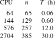
. Computation of the resulting eigenmode spectrum required only several terabytes of memory and approximately 600 cores on Cray XC30 (UK National High Performance Computing Facility), due to the efficient parallelization and scalability of the numerical algorithms for solving large non-symmetric generalized eigenvalue problems (table 1). In brief, the algorithm transforms the generalized eigenproblem (2.9) to the standard form
 $\unicode[STIX]{x1D63E}\widehat{{\bf\psi}}={\it\omega}\widehat{{\bf\psi}}$
, with
 $\unicode[STIX]{x1D63E}=\unicode[STIX]{x1D63D}^{-1}\unicode[STIX]{x1D63C}$
, and finds the Schur decomposition of
 $\unicode[STIX]{x1D63E}\unicode[STIX]{x1D650}=\unicode[STIX]{x1D650}\unicode[STIX]{x1D64E}$
computed via the QR iteration, where
 $\unicode[STIX]{x1D650}$
is an orthogonal matrix and
 $\unicode[STIX]{x1D64E}$
is an upper quasi-triangular matrix (with
 $1\times 1$
and
 $2\times 2$
diagonal blocks). Finally, the eigenvectors
 $\widehat{{\bf\psi}}$
are extracted from
 $\unicode[STIX]{x1D650}$
and
 $\unicode[STIX]{x1D64E}$
via triangular solves. All the computations are done in parallel with ScaLAPACK (Blackford et al.
Reference Blackford, Choi, Cleary, D’Azevedo, Demmel, Dhillon, Dongarra, Hammarling, Henry and Petitet1997) enriched with newly developed algorithms.
Execution time
 $T$
of the eigenvalue solver for problem (2.9) with complex-valued non-symmetric matrices
 $\unicode[STIX]{x1D63C}$
and
 $\unicode[STIX]{x1D63D}$
of the dimension
 $3n^{2}\times 3n^{2}$
; all timings are recorded on ARCHER (Cray XC30, the UK National Supercomputing Service).

Our eigenmode solving approach is a natural extension of the earlier studies, where either just two most unstable eigenmodes were found (Simonnet & Dijkstra Reference Simonnet and Dijkstra2002), or the whole spectrum was computed but on very coarse grids (Sheremet, Ierley & Kamenkovich Reference Sheremet, Ierley and Kamenkovich1997; Berloff Reference Berloff2005) thus limiting the outcome to only large eddy viscosity values. For example, Berloff (Reference Berloff2005) solved a similar problem on a
 $62^{2}$
horizontal grid. Here, we extend and continue previous studies, and (i) reach much higher spatial resolution, (ii) compute full spectrum of the eigenmodes and (iii) dynamically interpret the LFV in terms of the obtained eigenmodes.
3 Low-frequency variability of the midlatitude ocean and eigenmodes
In this section we employ the empirical orthogonal functions (EOF) analysis to extract the LFV of the flow and then apply the proposed method to obtain dynamical interpretation of the LFV.
3.1 LFV in the double gyres
The EOF analysis is a powerful tool for extracting spatially coherent and statistically significant transient variations from multivariable time series. In particular, this approach is efficient for the dimensionality reduction, compression and spatio-temporal variability analysis of atmospheric and oceanic data (Preisendorfer Reference Preisendorfer1988; Hannachi, Jolliffe & Stephenson Reference Hannachi, Jolliffe and Stephenson2007).
We applied the EOF method to extract the LFV of the statistically equilibrated, 100 year long QG solution, which has been low-pass filtered in time by a three-year running-window averaging and sampled on a
 $129^{2}$
uniform grid. It can be argued that in order to extract the LFV a low-pass filter can be used instead of the EOF method. However, the principal difference between using the EOFs and a low-pass filter is that the EOF method finds spatial patterns of variability most frequently realized in the solution, ranks them in terms of the variance and under the orthogonality constraint and gives a measure of the ‘importance’ of each pattern, while the low-pass filter merely cuts off the high-frequency component of the solution. In other words, the EOF method is one of the most optimal ways to pull out and rank in terms of importance all spatially coherent patterns of variability. The temporal variability of each coherent pattern is neither restricted nor imposed, but determined by the method.
For the extracted LFV we used the data of the upper-ocean streamfunction
 ${\it\psi}_{1}(t,x,y)$
, since most of the signal is localized in the upper ocean;
 ${\it\psi}_{1}$
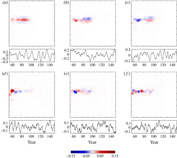
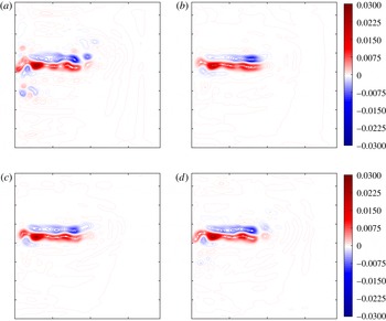
is used not only in the EOF method to extract LFV but also in the projection on the eigenmodes (see next section). There is no fundamental problem with extending the projection to all layers, if this is needed. We found that the upper ocean contains a robust large-scale 12 year LFV regime concentrated around the eastward jet. This LFV can be accurately approximated by the six leading EOFs and their principal components (PCs) (figure 2), that capture about 75 % of the total flow variability. As can be seen from figure 3, using 6 leading EOF–PC pairs in the approximation of the upper-layer velocity streamfunction are enough to accurately reconstruct the large-scale structure of the flow, and more accurate EOF–PC approximations do not lead to substantially more accurate results, although they enrich the flow with small-scale features, including some high-frequency components. These components are the intrinsic part of the solution but with small contribution to the LFV. The higher-order EOFs can be interpreted as meanders of the eastward jet, whereas the first and third EOFs, characterized by large time lag mutual correlations of
 $+$
0.52 and
 $-$
0.63 at
 $+$
3 and
 $-$
3 year lags, respectively, capture more than 40 % of the variability and determine the dominant 12 year period of the broadband LFV. This part of the signal is analogous to the ‘turbulent oscillator’ (Berloff et al.
Reference Berloff, Hogg and Dewar2007a
) and to the similar flow variability reported in Hogg et al. (Reference Hogg, Killworth, Blundell and Dewar2005). Thus, the turbulent oscillator is a robust phenomenon for the low-frequency behaviour in the midlatitude ocean circulation; it captures approximately 40 % of the variability and defines its dominant frequency. Detailed analysis of this LFV in more turbulent and higher-resolution flow regimes is beyond the scope of this paper.
Statistically extracted large-scale LFV of the eddying double gyres. Six leading, dimensionless empirical orthogonal functions (EOFs;
 $\text{EOF}_{1}$
(a),
 $\text{EOF}_{2}$
(b),
 $\text{EOF}_{3}$
(c),
 $\text{EOF}_{4}$
(d),
 $\text{EOF}_{5}$
(e),
 $\text{EOF}_{6}$
(f)) of the upper-layer velocity streamfunction
 ${\it\psi}_{1}$
and their principal components (below); contour interval is 0.01 (arbitrary units). These EOFs captures 75 % of the total variance of the flow fluctuations. Note that the amplitude of the EOFs gradually fades out (as the index of the EOF increases), so does its colour, since all EOFs are shown with the same colour scale.

Reconstruction of (a) the instantaneous upper-layer velocity streamfunction
 ${\it\psi}_{1}^{\prime }$
from (b) 6, (c) 12, and (d) 24 leading EOFs containing 75 %, 85 %, and 94 % of the upper-ocean flow variability, respectively; contour interval is 0.001 (arbitrary units). Note that using only 6 leading EOF–PC pairs in the approximation of the upper-layer velocity streamfunction is enough to accurately reconstruct the large-scale structure of the flow. Adding more EOF–PCs mainly enriches the flow reconstruction with small-scale details including some high-frequency components.

3.2 Projection of LFV onto eigenmodes
The EOF method’s skill in approximating the LFV with just a few statistical modes is contrasted by the lack of dynamical interpretation for these modes. To overcome this problem, we solved for the eigenmode spectrum of the linearized model (2.7), then, projected the 6-modes EOF–PC approximation of the LFV onto the eigenmodes and identified the contributing eigenmodes. It is important to note that nonlinear stresses estimated from the linear eigenmodes are often very good predictors of the actual nonlinear stresses. The number of examples is massive, ranging from classical textbooks to more recent results from geophysical turbulence (e.g. Berloff et al. Reference Berloff, Karabasov, Farrar and Kamenkovich2011; Berloff & Kamenkovich Reference Berloff and Kamenkovich2013a ,Reference Berloff and Kamenkovich b ; Davidson Reference Davidson2014; Dijkstra Reference Dijkstra2016).
The proposed method consists of three steps: (i) extracting the LFV in terms of EOF modes; (ii) finding the eigenmodes of the linearized dynamics; and (iii) projecting the LFV onto the set of relevant eigenmodes (note that the LFV is projected at different instants of time and covers all records of the solution). This approach is general enough and can be used for a wide spectrum of inhomogeneous turbulence problems with spatially varying background flows. Note that in homogeneous turbulence the eigenmodes are given by the Fourier modes that are a lot easier to deal with.
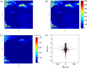
In order to project the extracted LFV onto the eigenmodes, we used the least-squares method, because the problem becomes overdetermined when the redundant eigenmodes are removed from the projection (see next section). Using the least-squares method can lead to some accuracy loss, especially for noisy data sets. To check the ability of this method to calculate accurate solutions, we carried out a number of numerical tests in which we selected eigenmodes with random numbers, assigned an arbitrary amplitude to each of these eigenmodes, and constructed an artificial flow by summing them up. Then, we used the least-squares method to project this flow on the eigenmodes with those randomly selected numbers and analysed the difference between the original and reconstructed flows. Our results show a high accuracy of the least-squares method (figure 4), thus proving it suitable for the projection algorithm.
Shown are (a) non-dimensional artificial flow constructed, on
 $127^{2}$
-grid, from 100 randomly selected eigenmodes with arbitrary amplitudes,
 $|{\it\psi}|$
; (b) artificial flow computed with the least-square method
 $|\widetilde{{\it\psi}}|$
; (c) difference between
 $|{\it\psi}|$
and
 $|\widetilde{{\it\psi}}|$
; (d) spectrum of the eigenproblem (2.9), the real and imaginary parts of the eigenvalue
 ${\it\omega}$
(
 $\text{year}^{-1}$
) correspond to the horizontal and vertical axis, respectively; eigenvalues corresponding to the selected eigenmodes are marked with red crosses. Although most of the selected eigenmodes are highly damped and noisy (due their proximity to the vertical axis of the spectrum) the least-squares method shows high accuracy, that makes it suitable for using in the projection algorithm.

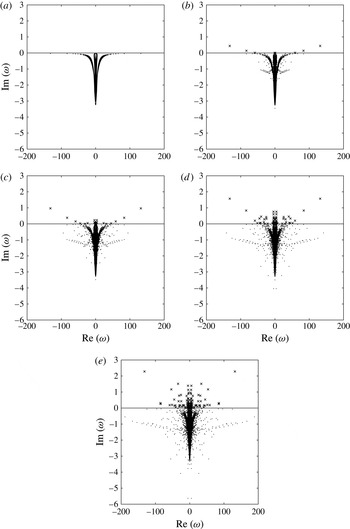
Evolution of the eigenmode spectrum for the fixed grid resolution of
 $65^{2}$
and gradually increasing flow intensity
 $I$
: (a)
 $I=0.0$
, (b)
 $I=0.25$
, (c)
 $I=0.5$
, (d)
 $I=0.75$
, (e)
 $I=1.0$
; stable and unstable eigenmodes are denoted by dots and crosses, respectively; the real and imaginary parts of the eigenvalue
 ${\it\omega}$
(
 $\text{year}^{-1}$
) correspond to the horizontal and vertical axis. Note that the flow intensity significantly influences the range of frequencies (the more intensive is the flow, the wider is the range), but has a minor effect on the range of eigenmode damping rates (almost no highly damped modes appear in the spectrum as the flow intensity increases).

We also estimated how both intensity of the flow and grid resolution affect the eigenmode characteristics, by solving the eigenproblem problem (2.9) with the gradually increasing flow intensity
 $I_{k}=\{0,0.25,0.50,0.75,1.00\}$
,
 $k=0,1,\ldots ,4$
and for the grid resolution fixed at
 $G=65^{2}$
, as well as on the other uniform grids with progressively increasing size
 $G_{k}=\{33^{2},65^{2},129^{2},257^{2}\}$
,
 $k=0,1,2,3$
.
As the flow intensity grows, so does the number of unstable modes, denoted as
 ${\it\sigma}^{+}$
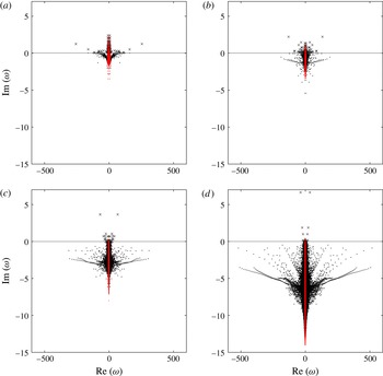
, (figure 5). On the contrary, as the resolution increases, the number of unstable eigenmodes gradually decreases (figure 6), and, thus, poorly resolved double gyres have even more unstable modes in the spectrum, because their viscous damping is underestimated. In particular, we found that
 ${\it\sigma}^{+}|_{I_{k}}=\{0,8,22,69,148\}$
,
 $k=0,1,\ldots ,4$
and
 ${\it\sigma}^{+}|_{G_{k}}=\{222,148,51,24\}$
,
 $k=0,1,2,3$
. Thus, we conclude that the reason for unstable eigenmodes to appear is the intensity of the background flow (the larger is the amplitude of the background flow, the more unstable modes appear in the spectrum) rather than the resolution. Note that although we work with numerically converged solutions in terms of the time-mean
 $l^{2}$
-norm relative error, the convergence in terms of the number of unstable modes
 ${\it\sigma}^{+}|_{G_{k}}$
is much stronger criterion and requires higher grid resolutions to be seen. We did not obtain the eigenmodes on the grids finer than those used for the eddying flow solutions, and further exploration of the resolution effects on the eigenmodes is beyond the scope of this paper.
Spectrum of the eigenproblem (2.9) for different grid resolutions: (a)
 $33^{2}$
, (b)
 $65^{2}$
, (c)
 $129^{2}$
, (d)
 $257^{2}$
. The removed part of the spectrum (80 % which is not used in the projection of LFV onto the eigenmodes) is marked by red colour; stable and unstable regimes are denoted by dots and crosses, respectively; the real and imaginary parts of the eigenvalue
 ${\it\omega}$
(
 $\text{year}^{-1}$
) correspond to the horizontal and vertical axis, respectively. The
 $257^{2}$
spectrum corresponds to the true grid used in the fully nonlinear model. Note that the eigenmodes become more damped as the grid resolution increases.

Another finding is that increasing flow intensity does not significantly elongate the spectrum, that results in a very small number of highly damped eigenmodes at low resolutions and high intensities of the flow. However, as the flow intensity increases, the spectrum widens, i.e. the range of frequencies becomes wider, and more and more fast eigenmodes come into play.
The situation with the spectrum on finer grids is different. As the grid is refined, the spectrum not only widens but also elongates (figure 6), thus showing increased damping rates of the eigenmodes. However, we found that these damped, long period, modes are not included in the LFV, while the short period ones are. The presence of the short period modes in the LFV is explained by the criterion we used to minimize the number of the eigenmodes the LFV is projected the best onto (see next section for more details).
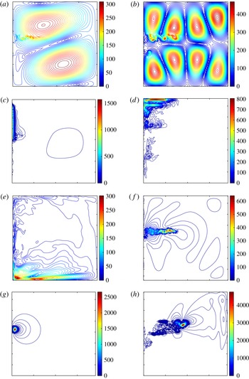
Classification of the eigenmodes and analyses of their interactions are beyond the scope of this paper, therefore, we restrict ourselves to exemplifying the most typical modes found (figure 7). As it can be seen, the LFV combines both large-scale basin-size modes (figure 7 a,b) and small-scale localized patterns (figure 7 c–h). Most of the small-scale modes are either boundary-trapped (figure 7 c–e) or eastward-jet-localized features (figure 7 f–h), and they can be interpreted as inhomogeneous Rossby waves that are strongly modified and controlled by the underlying large-scale flow. Most of these eigenmodes are stable, but with relatively slow damping rates, hence, they can be easily excited and maintained by interactions with other modes or by the wind forcing.
Spatial patterns of the eigenmodes. Non-dimensional amplitudes and frequencies
 ${\it\omega}$
(in units of (
 $\text{year}^{-1}$
)) of typical non-dimensional upper-layer eigenmodes
 $|{\it\psi}_{1}|$
used in the projection of the EOF-modes: (a) nearly barotropic mode,
 ${\it\omega}=-42.5-0.251\text{i}$
; (b) large-scale baroclinic mode,
 ${\it\omega}=-21.2-0.08\text{i}$
; (c) western-boundary trapped mode,
 ${\it\omega}=-58.7-2.9\text{i}$
; (d) northern-boundary trapped mode,
 ${\it\omega}=-4.0-1.5\text{i}$
; (e) southern-boundary trapped mode,
 ${\it\omega}=2.8-0.23\text{i}$
; (f) eastward-jet mode,
 ${\it\omega}=-30.8-2.7\text{i}$
; (g) jet-separation-point mode,
 ${\it\omega}=-155.2-1.0\text{i}$
and (h) jet-eastern-tip mode
 ${\it\omega}=10.5-2.4\text{i}$
. Contour interval is 10.0 (arbitrary units).

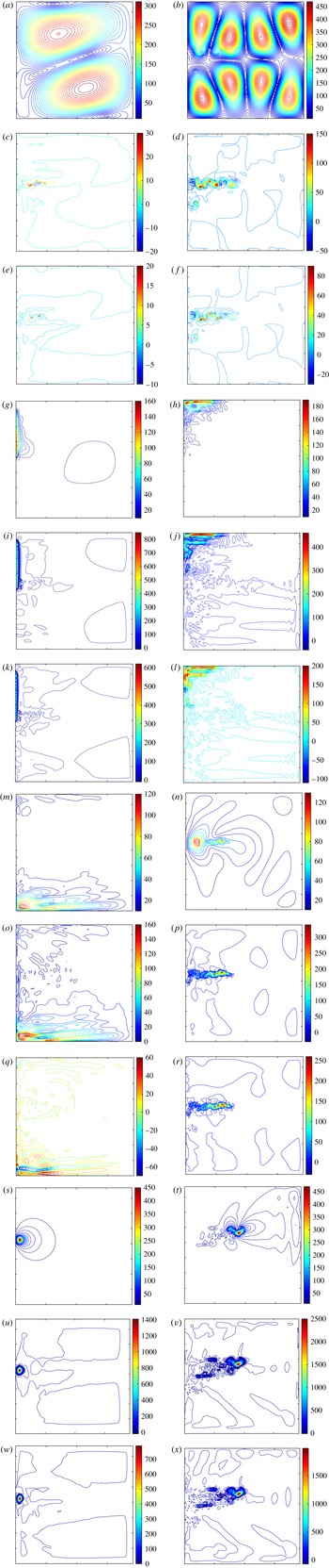
Vertically most of the eigenmodes are significantly mixed, because of the significant background flow effect. Thus, the modes are multiscale features both in horizontal and vertical directions (figure 8). The eigenmodes with significant basin-scale barotropic component contain significant small-scale baroclinic deformations around the eastward jet (figure 8 a–f). The large variety of scales contained in most of the eigenmodes makes them truly multiscale dynamical patterns that couple variability of the eastward jet to the largest available Rossby waves. Complete and systematic classification of the eigenmodes in terms of their multiscale contents is important but remains beyond the scope of this paper. Note that each eigenmode can be Fourier transformed and described in terms of the corresponding Fourier power spectrum and phase information, and such description will quantify its multiscale content.
Vertical structure of the eigenmodes. Projection of a typical eigenmode streamfunctions
 ${\it\psi}_{1}$
on the barotropic (BRT) (a,b,g,h,m,n,s,t), first (
 $\text{BCL}_{1}$
) (c,d,i,j,o,p,u,v) and second (
 $\text{BCL}_{2}$
) (e,f,k,l,q,r,w,x) baroclinic modes. Typical non-dimensional upper-layer eigenmodes used in the projection of the EOF-modes: (a,c,e) horizontally mixed nearly barotropic mode, (b,d,f) vertically and horizontally mixed mode, (g,i,k) western-boundary trapped mode, (h,j,l) northern-boundary trapped mode, (m,o,q) southern-boundary trapped mode, (n,p,r) eastward-jet mode, (s,u,w) jet-separation-point mode and (t,v,x) jet-eastern-tip mode, and contour interval is 10.0 (arbitrary units). By horizontally mixed modes we mean multiscale modes, i.e. with both large and small scales. All eigenmodes are normalized by the total energy. Note that the baroclinic fields clear exhibit small-scale patterns concentrated around the eastward jet. These baroclinic patterns are coupled to the well-structured large-scale barotropic fields characterized by very large (order of magnitude) spatial variations of the amplitude.

Our main result is that the LFV consists of very large number of eigenmodes, and these modes have very different characteristics. Almost all contributing eigenmodes have periods that are much shorter than the dominant LFV time scales, therefore, we conclude that the LFV is not a single-mode pattern, but it is a coherent pattern phenomenon consisting of a large number of short period phase-related eigenmodes interacting with each other.
3.3 Reconstruction of LFV from eigenmodes
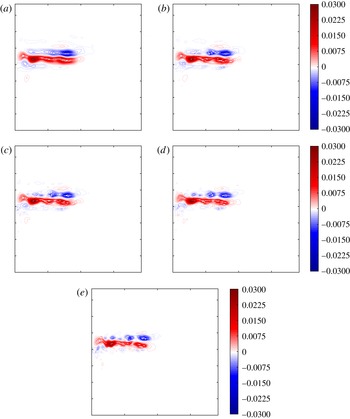
The projection of LFV onto eigenmodes begs the question as to how many eigenmodes are needed to reconstruct the LFV up to a given accuracy? To answer this question, we analysed different minimizing criteria and found that retaining the eigenmodes with the largest eigenfrequencies is the most efficient criterion leading to a minimal set of the eigenmodes. Other criteria we tried were based on retaining eigenmodes with the largest growth rates, or with the largest/smallest potential energy. In order to construct the minimal set of relevant eigenmodes, we gradually removed the eigenmodes with the smallest eigenfrequencies and tracked the accuracy of the projection of the LFV on the rest of the eigenmodes. It is clear that the more modes are removed from the projection the lower the projection accuracy becomes (figure 9). Our study shows that 20 % of the eigenmodes is required to keep the accuracy within a 15 % limit, and the accuracy is proportional to the grid resolution (table 2).
Degrading effect of the removed eigenmodes from the flow projections, as illustrated by arbitrary snapshots. Snapshot of the dimensionless upper-layer velocity streamfunction
 ${\it\psi}_{1}$
describing the LFV and consisting of the six leading EOFs is reconstructed from (a) 100 %, (b) 20 %, (c) 10 %, (d) 5 %, and (e) 2.5 % of the eigenmodes with the accuracy
 ${\it\delta}({\it\psi}_{1}^{(b)},{\it\psi}_{1}^{(a)})=16\,\%$
,
 ${\it\delta}({\it\psi}_{1}^{(c)},{\it\psi}_{1}^{(a)})=22\,\%$
,
 ${\it\delta}({\it\psi}_{1}^{(d)},{\it\psi}_{1}^{(a)})=28\,\%$
, and
 ${\it\delta}({\it\psi}_{1}^{(e)},{\it\psi}_{1}^{(a)})=39\,\%$
, respectively. Here, the superscript indicates the corresponding subfigure, and
 ${\it\delta}(f,g)=\Vert f-g\Vert _{2}/\Vert g\Vert _{2}$
is the
 $l^{2}$
-norm relative error with
 $f$
denoting the corresponding reconstructed
 ${\it\psi}_{1}$
, and
 $g$
standing for the reference solution
 ${\it\psi}_{1}^{(a)}$
; contour interval is 0.001 (arbitrary units). Note that all other snapshots provide a similar degrading effect.

Time-average
 $l^{2}$
-norm relative error
 ${\it\delta}(f,g)=\overline{\Vert f-g\Vert }_{2}/\overline{\Vert g\Vert }_{2}$
for different grid sizes
 $G$
in the spectral problem (2.8);
 $f$
is the flow reconstructed from the six leading EOF modes approximated by 20 % of the eigenmodes,
 $g$
is the reference solution. Our study shows that only 20 % of the eigenmodes is required to keep the accuracy within a 15 % limit, and the accuracy is proportional to the grid resolution.

Another finding is how the orthonormalization of the eigenmodes influences the projection accuracy (table 2). More specifically, we applied the Gram–Schmidt orthonormalization method to the eigenmodes, and thus turned them into orthonormalized modes (also called normal modes), and then projected the LFV onto such eigenmodes. Our results show a negligible difference in accuracy between the two projections, although the normal modes are not the individual solutions to the linearized dynamics. Thus, we conclude that using specifically tailored approximations of the generalized eigenvalue problem (2.9) which lead to the set of the orthonormalized modes yields no advantages, but results in the excessive complications of the numerical method and obscures the dynamical interpretations.
4 Conclusions
The goal of this work was to study the intrinsic large-scale LFV obtained in the eddy-resolving nonlinear model of the midlatitude ocean gyres, and to interpret it in terms of dynamically consistent (i.e. satisfying the formal dynamical constraints) eigenmodes of the corresponding linearized problem. The key question we asked is whether the LFV can be interpreted in terms of relatively few dynamically consistent modes, or even a single mode. Previous studies attempted such interpretations (e.g. see the review by Dijkstra (Reference Dijkstra2016)), but none of them were extended to highly nonlinear and turbulent flow regimes, such as the one considered in this paper.
With the EOF method applied, we extracted the LFV pattern and found, that it can be approximated by only six leading EOFs and their principal components. We also found that the LFV is predominantly decadal and concentrated around the eastward jet extension of the western boundary currents. Among the leading EOFs, we detected the LFV regime known as the ‘turbulent oscillator’ (Berloff et al. Reference Berloff, Hogg and Dewar2007a ).
In order to study the dynamical constituents of the LFV, we projected it onto the full spectrum of spatially inhomogeneous eigenmodes of the governing equations linearized around the time-mean flow solution of the nonlinear model. For the first time, by employing efficient and scalable computational methods, we were able to find the corresponding eigenmodes without any loss of accuracy, on the same computational grid as in the nonlinear eddy-resolving model. Note that because of the spatial inhomogeneity of the mesoscale eddy turbulence in the double gyres, these eigenmodes are very different from the Fourier modes that happen to be the homogeneous turbulence eigenmodes. We found that the LFV is a coherent structure phenomenon composed of the multitude of eigenmodes of different types and scales. Most of these modes have time scales significantly shorter than those suggested by the power spectrum of the PCs, therefore, their contributions come in terms of their nonlinear interactions. Most of the eigenmodes are multiscale patterns combining large and small horizontal length scales, and both barotropic and baroclinic vertical modes. This multiscale nature is mostly due to the background flow effect.
Another finding is that the number of unstable eigenmodes depends on the intensity of the background flow (the higher is the amplitude of the background flow, the more of the unstable modes appear in the spectrum) than on the grid resolution. However, the grid resolution affects both the range of frequencies (the higher the resolution the wider the range) and the damping rates (the higher the resolution the faster the damping rates become), while the flow intensity mostly influences the range of frequencies (the more intensive is the flow, the wider is the range), and induces only small changes in the damping rates.
An important future extension of this study is a classification of the eigenmodes in terms of their multiscale contents, partitioning of the eigenmode spectrum into distinct regions and systematic analysis of the linear and nonlinear interactions between the eigenmodes contributing to the nonlinear flow. Other future research avenues may study how the decreasing eddy viscosity affects the LFV and extend the proposed eigenproblem methodology to comprehensive ocean circulation models. Finally, our methodology can be significantly improved by application of non-uniform horizontal grids with spatially varying resolution.
Acknowledgements
The first two authors are thankful to the Natural Environment Research Council for the support of this work through the grant NE/J006602/1 and the use of ARCHER (the UK National Supercomputing Service). We express our gratitude to S. Burbidge and M. Harvey for their help with Imperial College London cluster, as well as to A. Thomas for his help with managing and maintaining the data storage. The last two authors were supported by the Spanish Ministry of Economy and Competitiveness under grant TIN2013-41049-P, and this support is gratefully acknowledged. We would also like to thank unknown referees for valuable comments and suggestions, which helped us to improve the paper.