1. Introduction
The Boltzmann equation is the fundamental equation in the study of rarefied gas dynamics that has found applications in space vehicle re-entry (Ivanov & Gimelshein Reference Ivanov and Gimelshein1998), microelectromechanical system processing (Karniadakis, Beskok & Aluru Reference Karniadakis, Beskok and Aluru2005), vacuum technology (Sharipov & Seleznev Reference Sharipov and Seleznev1998; Sone Reference Sone2002) and shale gas extraction (Wu et al. Reference Wu, Liu, Reese and Zhang2016, Reference Wu, Ho, Germanou, Gu, Liu, Xu and Zhang2017). In Boltzmann's description, all molecules move in straight lines with fixed velocities until they encounter elastic collisions with other molecules. The free transport is described by the streaming operator, while the binary collision is modelled by the Boltzmann collision operator (BCO), which is a nonlinear function of the velocity distribution function (VDF) and incorporates the effect of intermolecular potential. In the past century, the complicated structure of BCO has stimulated the development of kinetic models that strive to imitate as closely as possible the behaviour of the Boltzmann equation. In gas kinetic modelling, the streaming operator remains unchanged, while the BCO is replaced by simpler expressions, not only making the problems tractable, but also reducing the computational cost. For example, in the deterministic solver, the computational complexity of the BCO solved by the fast spectral method is approximately  $O(M^{2}N^{3}\log {N})$, where
 $N$ is the number of the discretised velocity grid in each velocity direction, and
 $M^{2}\sim {N}$ is the number of the discretised solid angle (Wu et al. Reference Wu, White, Scanlon, Reese and Zhang2013). However, the computational cost for the kinetic models is only
 $O(N^{3})$.
Several basic considerations are taken into account when simplifying the BCO (Struchtrup Reference Struchtrup2005). First, the conservation laws of mass, momentum and energy must be satisfied. Second, the VDF must be reduced to the Maxwellian equilibrium distribution when the gas system reaches equilibrium. Third, transport coefficients such as the viscosity and thermal conductivity derived from the kinetic model equation should coincide with those from the Boltzmann equation. Fourth, the H-theorem, which states that the production of entropy is always positive and vanishes only if the system is in equilibrium, should be satisfied. Note that the first two are basic physical requirements, and the third is crucial as it yields consistent solutions with the Boltzmann equation in the continuum flow regime (governed by the Navier–Stokes–Fourier equations). The fourth requirement determines whether the kinetic model works in a physical way and influences the stability/robustness, although it does not necessarily guarantee the accuracy of the kinetic model. Due to the complexity in mathematical analysis, there is often no strict proof of the H-theorem for existing kinetic models, e.g. the Shakhov (Reference Shakhov1968a,Reference Shakhovb) kinetic model where the H-theorem has not been proved in nonlinear cases. Nevertheless, the Shakhov model works well in many cases and is one of the most popular kinetic models.
In the Boltzmann equation, if the total cross-section is finite (either through the cut-off of impact parameter or from the quantum calculation), the collision operator can be decomposed into the gain term,  $Q^{+}$, and loss term,
 $\nu f$, as
 $Q=Q^{+} -\nu f$. Therefore, the modelled collision operator is often formulated in the relaxation-time approximation,
 \begin{equation} Q=\nu[f_{r}(t,\boldsymbol{v},\boldsymbol{x}) -f(t,\boldsymbol{v},\boldsymbol{x})], \end{equation}
where  $t$ is the time,
 $\boldsymbol {x}=(x_1,x_2,x_3)$ is the spatial coordinate,
 $\boldsymbol {v}=(v_1,v_2,v_3)$ is the molecular velocity,
 $\nu$ is the collision frequency (inverse relaxation time) and
 $f_{r}$ is the target VDF. Therefore, the two terms to be modelled are
 $f_{r}$ and
 $\nu$, which are connected with the gain and loss terms of the BCO, respectively. Many relaxation-type kinetic models assume
 $\nu$ to be a constant throughout the molecular velocity space and concentrate on the modelling of
 $f_{r}$. Three popular kinetic models of this kind are the BGK model (Bhatnagar, Gross & Krook Reference Bhatnagar, Gross and Krook1954), the ESBGK model (Holway Reference Holway1966) and the Shakhov model (Shakhov Reference Shakhov1968a). The BGK model cannot recover the shear viscosity and thermal conductivity simultaneously, hence it will not be discussed in this paper. The ESBGK model satisfies the H-theorem, while the Shakhov model satisfies the H-theorem only in linearised flows. Nevertheless, the ESBGK model by no means absolutely outperforms the Shakhov model: the Shakhov model is better in simulating the shock wave, Couette flow and Poiseuille flow, while the ESBGK model is better in some heat transfer problems (Liu & Zhong Reference Liu and Zhong2014; Chen, Xu & Cai Reference Chen, Xu and Cai2015; Ambruş, Sharipov & Sofonea Reference Ambruş, Sharipov and Sofonea2020).
It is noted that although these models assume velocity-independent collision frequency, the collision frequency of the BCO depends on the molecular velocity and this dependence influences the rarefied gas dynamics (Cercignani Reference Cercignani2000; Zheng & Struchtrup Reference Zheng and Struchtrup2005). For example, in the linearised Poiseuille flow and thermal transpiration, the Boltzmann equation yields different solutions for different intermolecular potentials even when the viscosity is same (Sharipov & Bertoldo Reference Sharipov and Bertoldo2009; Takata & Funagane Reference Takata and Funagane2011; Wu, Reese & Zhang Reference Wu, Reese and Zhang2014; Wu et al. Reference Wu, Liu, Zhang and Reese2015a). However, the ESBGK model and the Shakhov model do not have this capability: after linearisation their collision operators are only determined by the value of shear viscosity at some reference temperature.
To increase the accuracy of kinetic models, it would be highly desirable to add more information to the collision frequency and target VDF. Based on the eigenvalues and eigenfunctions of the linearised BCO for Maxwellian molecules, Gross & Jackson (Reference Gross and Jackson1959) proposed a systematic way to construct kinetic models with arbitrary order of accuracy. However, this is only limited to the linearised flow of Maxwellian gas. To be more general, the relaxation model (1.1) with velocity-dependent collision frequency becomes a natural consideration. To this end, kinetic models based on eigenfunctions of the linearised Boltzmann operator combined with variable collision frequency have been proposed by Cercignani (Reference Cercignani1966) and Loyalka & Ferziger (Reference Loyalka and Ferziger1967, Reference Loyalka and Ferziger1968); however, flows considered in the above studies are limited to the simple velocity and temperature slip problems where the variation of collision frequency has very limited influence on the slip coefficients. Relevant work has also been done by Larina & Rykov (Reference Larina and Rykov2007), but the linearised variable-collision-frequency model performs even worse than the constant-collision-frequency one. For the nonlinear case, Krook (Reference Krook1959) and Cercignani (Reference Cercignani1975) have mentioned a BGK-type model with velocity-dependent collision frequency and Maxwellian-type  $f_r$. This model is further developed by Struchtrup (Reference Struchtrup1997) and Mieussens & Struchtrup (Reference Mieussens and Struchtrup2004), where the collision frequency
 $\nu$ is some power-law function of the molecular velocity and the model is called the
 $\nu$-BGK model. The
 $\nu$-BGK model, however, fails to satisfactory predict the normal shock wave and the Couette flow. Zheng & Struchtrup (Reference Zheng and Struchtrup2005) then developed the
 $\nu$-ESBGK model, where a more physically meaningful collision frequency derived from the BCO is applied. It performs better than the
 $\nu$-BGK in the normal shock wave, but shows worse accuracy than the standard ESBGK model in the Couette flow. We also mention the recent work of Xu, Chen & Xu (Reference Xu, Chen and Xu2021), where a velocity-dependent collision frequency has been used in the particle-based unified gas-kinetic scheme and improved results in supersonic flows are observed.
Besides the relaxation-time approximations, the Fokker–Planck model (Jenny, Torrilhon & Heinz Reference Jenny, Torrilhon and Heinz2010; Gorji, Torrilhon & Jenny Reference Gorji, Torrilhon and Jenny2011; Gorji & Jenny Reference Gorji and Jenny2013) is another popular kinetic model. This model is applied to rarefied gas dynamics because, when compared with the direct simulation Monte Carlo method (DSMC) (Bird Reference Bird1994), it allows a much larger time step in the near-continuum flow regime where the Knudsen number ( $Kn$, the ratio of molecular mean free path to characteristic flow length)
 $Kn\ll 1$, and hence reduces the computational cost significantly. In terms of the model accuracy, despite its more complicated formulation, the Fokker–Planck model does not to have absolute advantage over relaxation-type models in the transition flow regime where
 $Kn\sim 1$. For instance, in the simulation of normal shock waves, it is found that the Fokker–Planck model works well for argon gas where the viscosity index is
 $\omega =0.81$, but its predication capability deteriorates for hard-sphere (HS) and Maxwell molecules (Liu et al. Reference Liu, Yuan, Javid and Zhong2019; Fei et al. Reference Fei, Liu, Liu and Zhang2020), where
 $\omega =0.5$ and 1, respectively. Moreover, like the BGK, ESBGK and Shakhov models, this model does not distinguish between the influence of intermolecular potentials in the simulation of Poiseuille flow and thermal transpiration (Sharipov & Bertoldo Reference Sharipov and Bertoldo2009), as well as the Rayleigh–Brillouin scattering (Wu et al. Reference Wu, White, Scanlon, Reese and Zhang2015b).
In view of the above facts, we aim to further develop the relaxation model (1.1) with velocity-dependent collision frequency to recover more details of the BCO, while keep the computation complexity in an affordable level. The  $\nu$-model we propose adopts the velocity-dependent collision frequency based on the equilibrium collision frequency of the BCO with empirical modification. The influence of intermolecular potential (Sharipov & Bertoldo Reference Sharipov and Bertoldo2009) is appropriately accounted for, including the Lennard-Jones potential which is accurate in a wide range of temperatures. To recover the correct Prandtl number, considering that in our most concerned cases the Shakhov model outperforms the ESBGK model (Liu & Zhong Reference Liu and Zhong2014; Chen et al. Reference Chen, Xu and Cai2015; Ambruş et al. Reference Ambruş, Sharipov and Sofonea2020), a Shakhov-type target VDF is employed. With these two critical improvements, we find that the model accuracy is greatly improved; moreover, the multiscale numerical method that is efficient from the continuum to free-molecular flow regimes can be adopted, and the computational cost only increases slightly when compared with conventional kinetic models.
The rest of the paper is organised as follows. The Boltzmann equation, as well as the transport coefficients and equilibrium collision frequency, are introduced in § 2. In § 3, different kinetic models with velocity-independent or velocity-dependent collision frequency are introduced, and our  $\nu$-model is proposed. Section 4 describes the numerical method used to solve the proposed model equation. In §§ 5 and 6, the accuracy of our kinetic model is assessed by numerous canonical test cases and the underlying mechanisms on how the
 $\nu$-model improves the results are discussed. Summaries and outlooks are given in § 8.
2. The Boltzmann equation
A kinetic model is proposed to imitate the behaviour of the Boltzmann equation. Therefore, some basic properties of the Boltzmann equation, including the differential cross-section, the intermolecular potential, the link to transport coefficients and the equilibrium collision frequency are introduced. These form the theoretical basis of constructing kinetic models.
A fundamental theory at the mesoscopic level that bridges the microscopic and mesoscopic behaviours is much required to describe the rarefied gas dynamics. As we are not interested in the individual dynamics of gas molecules but their collective behaviours, the VDF  $f(t,\boldsymbol {x},\boldsymbol {v})$ is introduced to describe the state of the gas. It is defined in such a way that the quantity
 $f(t,\boldsymbol {x},\boldsymbol {v})\, {{\rm d}}\kern0.7pt \boldsymbol {x}\, {{\rm d}} \boldsymbol {v}$ is the molecular number in the phase-space volume
 ${\rm d}\kern0.7pt \boldsymbol {x}\, {{\rm d}} \boldsymbol {v}$. Therefore, macroscopic quantities such as the molecular number density
 $n(t,\boldsymbol {x})$, flow velocity
 $\boldsymbol {u}(t,\boldsymbol {x})$, temperature
 $T(t,\boldsymbol {x})$, pressure tensor
 $p_{ij}(t,\boldsymbol {x})$ and heat flux
 $\boldsymbol {q}(t,\boldsymbol {x})$ can be calculated as
 \begin{equation} [n,\boldsymbol{u}, T, p_{ij}, \boldsymbol{q}]=\int \left[1,\frac{\boldsymbol{v}}{n}, \frac{m}{3k_Bn(t,x)}c^{2},mc_ic_j,\frac{m}{2}c^{2} \boldsymbol{c}\right]f(t,\boldsymbol{x},\boldsymbol{v})\, {{\rm d}} \boldsymbol{v}, \end{equation}
where  $\boldsymbol {c}=\boldsymbol {v}-\boldsymbol {u}$ is the peculiar velocity,
 $k_B$ is the Boltzmann constant, and
 $m$ is the molecular mass. Note that the ideal gas law holds for dilute gas, where the gas pressure is
 $p=nk_BT$. Also, we introduce the pressure deviation tensor
 $\sigma _{ij}$ as
 $\sigma _{ij}=p_{ij}-p\delta _{ij}$, where
 $\delta$ is the Kronecker delta.
In the absence of external force, the Boltzmann equation reads
 \begin{equation} \frac{\partial {f}}{\partial{t}}+{\boldsymbol{v}}\boldsymbol{\cdot}\frac{\partial {f}}{\partial{\boldsymbol{x}}}= \iint B(|\boldsymbol{v}_r|,\theta) [f(t,\boldsymbol{x},\boldsymbol{v}'_\ast)f(t,\boldsymbol{x}, \boldsymbol{v}')-f(t,\boldsymbol{x},\boldsymbol{v}_\ast)f(t, \boldsymbol{x},\boldsymbol{v})]\, {{\rm d}} \varOmega \, {{\rm d}} {\boldsymbol{v}}_\ast, \end{equation}
where the term in the right-hand side is the BCO. The subscript  $\ast$ represents the second molecule in the binary collision, the superscript
 $'$ stands for quantities after the collision,
 $\boldsymbol {v}_r=\boldsymbol {v}-\boldsymbol {v}_\ast$ is the relative precollision velocity and
 $\theta$ is the deflection angle. The postcollision molecular velocities are given by
 $\boldsymbol {v}'=\boldsymbol {v}+({|\boldsymbol {v}_r|\varOmega - \boldsymbol {v}_r})/{2}$ and
 $\boldsymbol {v}'_\ast =\boldsymbol {v}_\ast - ({|\boldsymbol {v}_r|\varOmega -\boldsymbol {v}_r})/{2}$, with
 $\varOmega$ being the unit vector in the direction of the solid angle. The deflection angle
 $\theta$ between the precollision and postcollision relative velocities satisfies
 $\cos \theta = \varOmega \boldsymbol {\cdot }\boldsymbol {v}_r/|\boldsymbol {v}_r|$,
 $0\le \theta \le {\rm \pi}$.
The collision kernel  $B(|\boldsymbol {v}_r|,\theta )$ in the BCO is a product of the differential cross-section
 $\sigma _D$ and the relative collision speed,
 \begin{equation} B(|\boldsymbol{v}_r|,\theta)=\sigma_D|\boldsymbol{v}_r| \equiv\frac{b|{{\rm d}}b|}{\sin\theta|{{\rm d}} \theta|}|\boldsymbol{v}_r|, \end{equation}
which is always non-negative. Note that the calculation of  $\sigma _D$ follows the classical mechanics, since when the gas temperature is not too low, both the classical mechanics and quantum mechanics yield the same transport coefficients (Sharipov & Benites Reference Sharipov and Benites2017). Given the intermolecular potential
 $\phi$, the deflection angle is calculated based on the impact parameter
 $b$ and the relative velocity
 $|\boldsymbol {v}_r|$, as follows:
 \begin{equation} \theta(b,{v}_r)={\rm \pi}-2\int_0^{W_1}\left[1-W^{2}- \frac{4\phi(r)}{m{v}_r^{2}}\right]^{{-}1/2}\, {{\rm d}}W, \end{equation}
where  $W=b/r$ with
 $r$ being the intermolecular distance and
 $W_1$ is positive root of the term in brackets. In gas kinetic theory, the inverse power-law potentials are normally considered,
 \begin{equation} \phi(r)=\frac{K}{\eta-1}r^{1-\eta}, \end{equation}
although the Lennard-Jones potential is more realistic (it is widely used in the molecular dynamics simulation),
 \begin{equation} \phi(r)=4\epsilon\left[\left(\frac{d_{LJ}}{r}\right)^{12}- \left(\frac{d_{LJ}}{r}\right)^{6}\right], \end{equation}
where  $\epsilon$ is the potential depth, and
 $d_{LJ}$ is the distance between two molecules where the potential is zero. The power-law potentials are called hard- and soft-potentials when
 $\eta >5$ and
 $\eta <5$, respectively. Maxwell molecules have the potential with
 $\eta =5$. Another special case is the HS gas, where the repulsive potential is infinity (and zero) when
 $r$ is less (larger) than the molecular diameter
 $\sigma$.
For the power-law potential, it is seen from (2.4) that the deflection angle is only a function of
 \begin{equation} s=\left[\frac{m(\eta-1)}{4K}\right]^{{1}/({\eta-1})}bv^{{2}/({\eta-1})}_r. \end{equation}
That is,  $\theta =\theta (s)$. Thus, the differential cross-section is
 \begin{equation} B(|\boldsymbol{v}_r|,\theta)=\left[\frac{m(\eta-1)}{4K} \right]^{{2}/({1-\eta})}v^{({\eta-5})/({\eta-1})}_r \times\underbrace{\frac{s\, {{\rm d}}s}{\sin\theta{{{\rm d}} \theta}}}_{\varTheta(\theta)}. \end{equation}
For Maxwell molecules, the collision kernel is independent of the relative collision speed, while for HS gas the collision kernel is independent of the deflection angle:  $B(|\boldsymbol {v}_r|,\theta )=({\sigma ^{2}}/{4})|\boldsymbol {v}_r|.$
2.1. Transport coefficients and modelled collision kernel
The collision kernel  $B(|\boldsymbol {v}_r|,\theta )$ determines the transport coefficients such as the shear viscosity and thermal conductivity. In the continuum flow regime, the Navier–Stokes–Fourier equations can be derived from the Chapman–Enskog expansion of the Boltzmann equation, where the shear viscosity, when the leading order in the Sonnie expansion is considered, is given by (Chapman & Cowling Reference Chapman and Cowling1970)
 \begin{equation} \mu=\frac{5\sqrt{{\rm \pi}{m}k_BT}}{8D},\quad D = 2{\rm \pi} {\left( {\frac{m}{{4{k_B}T}}} \right)^{4}}\int_0^{\infty} {\int_0^{\rm \pi} {v_r^{7}{\sigma _D}{{\sin }^{3}}\theta \exp \left( { - \frac{{mv_r^{2}}}{{4{k_B}T}}} \right)\, {{\rm d}} \theta \, {{\rm d}} {v_r}} } . \end{equation}
The corresponding thermal conductivity is given by
 \begin{equation} {\kappa}=\frac{15}{4}\frac{k_B}{m}\mu, \end{equation}
which results in a Prandtl number of  $Pr =({5k_B}/{2m})({\mu }/{\kappa })=\frac {2}{3}$.
Therefore, for the inverse-power potential, we have  $\mu \propto {T^{\omega }}$, where
 \begin{equation} \omega=\frac{\eta+3}{2(\eta-1)}, \end{equation}
is the viscosity index; for the Lennard-Jones potential, the viscosity is not a power-law function of the temperature, since  $D$ is approximated by (Wu et al. Reference Wu, White, Scanlon, Reese and Zhang2013)
 \begin{equation} \frac{D}{d_{LJ}^{2}}=b_1\left(\frac{k_BT}{\epsilon}\right)^{{-}0.4} +b_2 \left(\frac{k_BT}{\epsilon}\right)^{{-}0.45}+b_3 \left(\frac{k_BT}{\epsilon}\right)^{{-}0.5}, \end{equation}
where  $b_1=407.4, b_2=-811.9$ and
 $b_3=414.4$; each term can be viewed as the inverse power-law potential with the viscosity indices
 $\omega _1=0.9$,
 $\omega _2=0.95$ and
 $\omega _3=1$, respectively. Note that this approximation is accurate when
 $1< k_BT/\epsilon <25$.
In the DSMC method (Bird Reference Bird1963) and the fast spectral approximation of the BCO (Wu et al. Reference Wu, White, Scanlon, Reese and Zhang2013), the modelled collision kernels such as the variable HS and variable soft-sphere models are used: the transport coefficients are recovered, but the detailed form of  $\varTheta (\theta )$ in (2.8) is modified to make the computation simple. For example, in the inverse power-law and Lennard-Jones potentials, the modelled collision kernel are, respectively,
 \begin{align} \left.\begin{array}{c@{}}
B=\dfrac{5\sqrt{{\rm \pi}{m}k_BT_0}(4k_BT_0/m)^{(1-\alpha)/2}}{64{\rm \pi}
\mu(T_0)\varGamma[(3+\alpha+\gamma)/2]\varGamma(2-\gamma/2)}
\sin^{\alpha+\gamma-1}\left(\dfrac{\theta}{2}\right)
\cos^{-\gamma}\left(\dfrac{\theta}{2}\right)
|\boldsymbol{v}_r|^{\alpha},\\ \displaystyle
B=\dfrac{d_{LJ}^{2}}{8{\rm \pi}}\sum_{j=1}^{3}
\dfrac{({m}/{4\epsilon})^{(\alpha_j-1)/2}}{\varGamma
\left(\dfrac{3+\alpha_j}{2}\right)}b_j
\sin^{\alpha_j-1}\left(\dfrac{\theta}{2}\right)
|\boldsymbol{v}_r|^{\alpha_j}, \end{array}\right\}
\end{align}
where  $\varGamma$ is the gamma function,
 $\mu (T_0)$ is the shear viscosity at the reference temperature
 $T_0$,
 \begin{equation} \alpha=\frac{\eta-5}{\eta-1}=2(1-\omega), \end{equation}
and  $\alpha _1=0.2, \alpha _2=0.1$ and
 $\alpha _3=0$. Note that
 $\gamma$ is a free parameter, the different value of which leads to different value of equilibrium collision frequency but always the same value of shear viscosity.
2.2. Equilibrium velocity distribution and collision frequency
It is well known that in equilibrium the BCO vanishes, and the VDF takes the form of the Maxwellian distribution
 \begin{equation} F_{eq}=n\left(\frac{m}{2{\rm \pi} k_BT}\right)^{3/2}\exp\left(-\frac{mc^{2}}{2k_BT}\right). \end{equation}
If the total cross-section is finite (either through the cut-off of impact parameter or from the quantum calculation of differential cross-section), the BCO can be separated into a gain term  $Q^{+}$ and a loss term
 $\nu {f}$ as
 $Q(f,f_*)=Q^{+} -\nu (|\boldsymbol {v}|){f}$, where the collision frequency is
 \begin{equation} \nu(|\boldsymbol{v}|)=\iint B(|\boldsymbol{v}_r|,\theta) f(\boldsymbol{v}_{{\ast}}) \, {{\rm d}} \varOmega \, {{\rm d}} \boldsymbol{v}_\ast. \end{equation}
For inverse power-law potentials, the equilibrium collision frequency corresponding to the collision kernel (2.8) and equilibrium VDF (2.15) is (Struchtrup Reference Struchtrup2005)
 \begin{align} \nu_{eq}(|\boldsymbol{v}|)\!=\!2{\rm \pi}\frac{\eta\!-\!1}{3\eta\!-\!7}\nu_\eta^{0} \underbrace{\int_0^{\infty} \frac{\xi_\ast}{\xi}\exp(\!-\!\xi^{2}_\ast) [ (\xi+\xi_\ast)^{({3\eta-7})/({\eta-1})} -|\xi-\xi_\ast|^{({3\eta-7})/({\eta-1})}] \, {{\rm d}} \xi_\ast}_{\nu^{0}_{eq}}, \end{align}
where
 \begin{align} \left.\begin{array}{c@{}}
\displaystyle
\nu_\eta^{0}=\left[\dfrac{m(\eta-1)}{4K}\right]^{{2}/({1-\eta})}
\dfrac{2n}{\sqrt{\rm \pi}}\sqrt{\dfrac{2k_BT}{m}}^{({\eta-5})/({\eta-1})}
\int s\, {{\rm d}}s,\\ \displaystyle
\nu_{HS}^{0}=n\sqrt{\dfrac{2k_BT}{m{\rm \pi}}}\sigma^{2}
\end{array} \right\}
\end{align}
and  $\xi ={c}/{v_m}$ with
 \begin{equation} v_m=\sqrt{\frac{2k_BT}{m}}, \end{equation}
being the most probable speed at temperature  $T$.
Specifically, for Maxwellian molecules with  $\eta =5$, the collision frequency is independent of the molecular velocity, and independent of the temperature:
 $\nu _{eq}={\rm \pi} ^{3/2}\nu _5^{0}$, while for HS molecules,
 \begin{equation} \nu_{eq}(|\boldsymbol{v}|)=n\sqrt{\frac{2{\rm \pi}{k_B}T}{m}}\sigma^{2} \underbrace{ \left[ \exp(-\xi^{2})+\frac{\sqrt{\rm \pi}}{2} \left(\frac{1}{\xi}+2\xi\right)\text{erf}(\xi) \right]}_{2\nu^{0}_{eq}/3}, \end{equation}
where  $\textrm {erf}(x)$ is the Gauss error function.
3. Kinetic models
In this section we first introduce the popular kinetic models with velocity-independent collision frequency and the history of kinetic models with velocity-dependent collision frequency, which helps to understand the line of thought in constructing the present kinetic model. Then we give details of our new variable-collision-frequency kinetic model. All models involved share the same form of (1.1).
3.1. Velocity-independent collision frequency
From (1.1) we can see that, in the velocity-independent collision-frequency model, the only term to be modelled is the target VDF  $f_{r}$, which is connected with the gain term of the BCO and directly determines the velocity distribution of the postcollision molecules. The BGK model (Bhatnagar et al. Reference Bhatnagar, Gross and Krook1954) adopts the local Maxwellian
 $F_{eq}$ to approximate
 $f_{r}$ and is the simplest kinetic model being widely used. One can verify that it satisfies the conservation laws. Also, in the equilibrium where the collision operator vanishes,
 $f=F_{eq}$, which fulfils the second requirement of kinetic modelling. The H-theorem can also be proved. However, from the Chapman–Enskog expansion, it can be found that the shear viscosity and thermal conductivity are
 \begin{equation} \mu=\frac{p}{\nu}, \quad \kappa=\frac{p}{\nu}\frac{5k_B}{2m}, \end{equation}
which results in a Prandtl number of unity. That is to say, the BGK model cannot recover the viscosity and thermal conductivity simultaneously. Therefore, many kinetic models have been proposed to correct the Prandtl number, among which the ESBGK model (Holway Reference Holway1966) and the Shakhov model (Shakhov Reference Shakhov1968a,Reference Shakhovb) are two of the most popular kinetic models.
In the ESBGK model of Holway (Reference Holway1966), the target VDF is obtained by maximising the entropy function  $H=-\int {f\ln }f\, {\textrm {d}} \boldsymbol {v}$ under the given information of mass, momentum, energy and the stress tensor. This can be finished by the Lagrange multipliers method and the target VDF finally has a form of an anisotropic Gaussian,
 \begin{equation} f_r^{ES}=\frac{n}{\sqrt{\operatorname{det} [2{\rm \pi}\lambda_{ij}]}}\exp\left(-\frac{1}{2}\lambda_{ij}^{{-}1}c_i{c_j}\right), \end{equation}
where
 \begin{equation} \lambda_{ij}=\frac{k_BT(1-b)}{m}\delta_{ij}+ \frac{bp_{ij}}{nm}=\frac{p\delta_{ij}+b\sigma_{ij}}{nm}, \end{equation}
with a constant  $b$. If
 $b=0$,
 $\lambda _{ij}$ becomes diagonal, and the BGK model is recovered. According to the Chapman–Enskog expansion, the transport coefficients are
 \begin{equation} \mu=\frac{p}{\nu(1-b)}, \quad \kappa=\frac{p}{\nu}\frac{5k_B}{2m}. \end{equation}
Therefore,  $b$ should take the value of
 $-\frac {1}{2}$ to produce a Prandtl number of
 $\frac {2}{3}$ for monatomic gas.
The ESBGK model satisfies the mass, momentum and energy conservations, as well as the H-theorem (Andries et al. Reference Andries, Tallec, Perlat and Perthame2000). At first sight it may appear that the VDF is guided towards the target one which is not the equilibrium distribution. However, in spatial-homogeneous problems we have
 \begin{equation} \frac{\partial \sigma_{ij}}{\partial t}={-}\frac{p}{\mu}\sigma_{ij}, \end{equation}
which means that the deviational stress will decay to zero. Thus, the route to equilibrium of the ESBGK model is as follows: as  $f$ approaches
 $f_r^{ES}$,
 $f_r^{ES}$ itself approaches
 $F_{eq}$ as per (3.2) and (3.3); eventually
 $f=F_{eq}$ when the equilibrium state is reached. Therefore, the ESBGK model satisfies all the four requirements of kinetic modelling detailed in § 1, and it has attracted much attention.
In contrast to the ESBGK model where the stress tensor is introduced in the target VDF, in the Shakhov model the heat flux is introduced on top of the BGK model (Shakhov Reference Shakhov1968a,Reference Shakhovb) through the Hermite polynomial,
 \begin{equation} f_r^{S}=F_{eq}\left[1+(1-{Pr})\frac{2m\boldsymbol{q}\boldsymbol{\cdot} \boldsymbol{c}}{5n(k_BT)^{2}}\left(\frac{mc^{2}}{2k_BT}-\frac{5}{2}\right)\right], \end{equation}
where the two transport coefficients are
 \begin{equation} \mu=\frac{p}{\nu}, \quad \kappa=\frac{1}{{Pr}}\frac{5k_B}{2m}\frac{p}{\nu}. \end{equation}
Thus, the correct value of the Prandtl number is recovered. The route to equilibrium of the Shakhov model is as follows: as  $f$ approaches
 $f_r^{S}$,
 $f_r^{S}$ itself approaches
 $F_{eq}$ since in spatial-homogeneous problems the heat flux decays to zero according to the equation
 \begin{equation} \frac{\partial \boldsymbol{q}}{\partial t}={-}\frac{2}{3}\frac{\mu}{p}\boldsymbol{q}. \end{equation}
Eventually  $f=F_{eq}$ when the equilibrium state is reached.
Comparing with the ESBGK model, the Shakhov model has two shortcomings. First, the H-theorem can be proved only for linearised flows, while one can neither prove nor disprove the H-theorem in nonlinear flows. Second, the VDF may become negative, which is not physical. However, despite the two deficiencies, the Shakhov model has been widely used, and it outperforms the ESBGK model in some cases.
3.2. Velocity-dependent collision frequency
Kinetic models with velocity-dependent collision frequency have been investigated in very early years. For the linearised Boltzmann equation, Cercignani (Reference Cercignani1966) and Loyalka & Ferziger (Reference Loyalka and Ferziger1967, Reference Loyalka and Ferziger1968) presented variable-collision-frequency models based on eigenfunctions of the linearised operator. These models are applied to simple velocity and temperature slip problems, and a limited influence on the slip coefficient due to the variation of collision frequency has been found. Larina & Rykov (Reference Larina and Rykov2007) have also developed a linearised model with velocity-dependent collision frequency, but in the simulation of normal shock waves, their model performs even worse than its constant-collision-frequency counterpart. For the nonlinear case, Krook (Reference Krook1959) and Cercignani (Reference Cercignani1975) have mentioned a variable-collision-frequency model where the target VDF is approximated as a Maxwellian with modified density, velocity and temperature determined by the collision conservation condition. Further investigations about this model have been done by Struchtrup (Reference Struchtrup1997) and Mieussens & Struchtrup (Reference Mieussens and Struchtrup2004), where the collision frequency is some power-law function of the molecular velocity; the model is called the  $\nu$-BGK model, but the numerical results for normal shock wave are not satisfactory.
It is interesting to note that although the original motivation of developing kinetic models with velocity-dependent collision frequency is to correct the Prandtl number of the standard BGK model, it is found that setting  $\nu$ to be the equilibrium collision frequency of the Boltzmann equation in the
 $\nu$-BGK model leads to an approximate unit Prandtl number (Mieussens & Struchtrup Reference Mieussens and Struchtrup2004). This suggests that the wrong Prandtl number of the standard BGK model is mainly due to the error in target VDF
 $f_{r}$ (the gain term), but not the error of collision frequency (the loss term). Therefore, it is less important to adjust the Prandtl number through modifying the collision frequency
 $\nu$. In contrast, one should modify the target VDF to guarantee a correct Prandtl number while applying a physically meaningful collision frequency. This has been done by Zheng & Struchtrup (Reference Zheng and Struchtrup2005) in their
 $\nu$-ESBGK model, where the equilibrium collision frequency is applied and an ESBGK-type target VDF is adopted to adjust the Prandtl number. The
 $\nu$-ESBGK model performs better than the
 $\nu$-BGK and ESBGK models in shock wave simulations, but performs worse than standard ESBGK in Couette flow (Zheng & Struchtrup Reference Zheng and Struchtrup2005).
3.3. New kinetic model with velocity-dependent collision frequency
Here we propose a new kinetic model with velocity-dependent collision frequency, that we call the  $\nu$-model. We design the target VDF as
 \begin{equation} f_r=\left[\hat{\varrho}+\hat{\varGamma}c^{2}+\gamma_ic_i +\beta\frac{2m\boldsymbol{q}\boldsymbol{\cdot} \boldsymbol{c}}{5n(k_BT)^{2}} \left(\frac{mc^{2}}{2k_BT}-\frac{5}{2}\right) \right] F_{eq}, \end{equation}
where  $\hat {\varrho }$,
 $\hat {\varGamma }$ and
 $\gamma _i$ are velocity independent, which can be solved directly from the conservation condition. Note that in the
 $\nu$-BGK model (Mieussens & Struchtrup Reference Mieussens and Struchtrup2004),
 $\hat {\varGamma }$ and
 $\gamma _i$ appear in the exponential function so Newton's iteration method should be applied; here we put them in the brackets to avoid the use of Newton's iteration method in the numerical simulation. The heat flux term as in the Shakhov model is used, and the velocity-independent parameter
 $\beta$ is used to adjust the Prandtl number. Thus, the collision frequency can be an arbitrary function of the molecular velocity. When
 $\nu$ is velocity-independent, this model will be reduced to the Shakhov (Reference Shakhov1968a,Reference Shakhovb) model.
We choose an isotropic velocity-dependent collision frequency  $\nu (|\boldsymbol v|)$. Applying the Chapman–Enskog expansion, the VDF to the first-order approximation reads
 \begin{align} f&=F_{eq}(\hat{\varrho}+\hat{\varGamma}c^{2}+\gamma_ic_i) +F_{eq}\beta\frac{2m\boldsymbol{q}\boldsymbol{\cdot} \boldsymbol{c}}{5n(k_BT)^{2}} \left(\frac{mc^{2}}{2k_BT}-\frac{5}{2}\right) \nonumber\\ &\quad -\frac{F_{eq}}{\nu(|\boldsymbol v|)} \left\{ \frac{m}{k_BT}\frac{\partial u_{\langle i}}{\partial x_{j\rangle}} c_{\langle i}c_{j\rangle} +\frac{1}{T}\frac{\partial T}{\partial x_i}c_i\left(\frac{mc^{2}}{2k_BT}-\frac{5}{2}\right) \right\}, \end{align}
where  $\hat {\varrho }=1, \hat {\varGamma }=0$ and
 \begin{equation} \gamma_i=\frac{8}{3\sqrt{\rm \pi}}\frac{1}{T}\frac{\partial{T}}{\partial{x_i}} \int_0^{\infty}\frac{\xi^{4}}{{\nu}(\xi)}\left(\xi^{2}-\frac{5}{2}\right) \exp(-\xi^{2})\, {{\rm d}} {\xi}. \end{equation}
Therefore, the shear viscosity and thermal conductivity are
 \begin{align} \left.\begin{array}{c@{}}
\displaystyle \mu=\dfrac{16p}{15\sqrt{\rm \pi}}\int_0^{\infty}
\dfrac{\xi^{6}}{\nu(\xi)}\exp(-\xi^{2})\, {{\rm d}}
{\xi},\\ \displaystyle
\kappa=\dfrac{1}{1-\beta}\dfrac{16p}{15\sqrt{\rm \pi}}
\dfrac{5k_B}{2m}\int_0^{\infty} \dfrac{\xi^{4}
\left(\xi^{2}-\dfrac{5}{2}\right)^{2}}{\nu(\xi)}\exp(-\xi^{2})\,
{{\rm d}} {\xi}. \end{array}\right\}
\end{align}
Thus, to recover the viscosity, an arbitrary positive collision frequency function  $v'(\xi )$ can be used in the
 $\nu$-model with the normalisation
 \begin{equation} \nu (\xi ) = A\frac{p}{\mu }\nu '(\xi ), \quad A = \frac{{16}}{{15\sqrt {\rm \pi}}}\int_0^{\infty} \frac{1}{{\nu '(\xi )}}{\xi ^{6}} \, {\rm e}^{ - {\xi ^{2}}}\, {{\rm d}} \xi , \end{equation}
and to recover the thermal conductivity, the parameter  $\beta$ can be calculated based on the Prandtl number
 \begin{equation} \beta = 1 - Pr \frac{\displaystyle {{{\int_0^{\infty} {\frac{{{\xi ^{4}}}}{{\nu ' (\xi )}}\left( {{\xi ^{2}} - \frac{5}{2}} \right)} }^{2}}\exp ( - {\xi ^{2}})\, {{\rm d}} \xi }}{\displaystyle {\int_0^{\infty} {\frac{{{\xi ^{6}}}}{{\nu ' (\xi )}}\exp ( - {\xi ^{2}})\, {{\rm d}} \xi } }}. \end{equation}
As for the velocity-dependent collision frequency  $\nu (\xi )$, as analysed above there are many forms to be chosen. In the current work, a half-theoretical and half-empirical formula has been established for
 $\nu (\xi )$, which will be discussed in § 5.1.
It is clear that the  $\nu$-model satisfies the conservation laws. Also, the VDF can be properly relaxed to the Maxwellian distribution (2.15), because when the equilibrium is reached the heat flux vanishes in a way similar to (3.8), meanwhile according to (3.11) there will be
 $\hat {\varrho }=1, \hat {\varGamma }=0, \gamma _i=0$, and finally the target VDF (3.9) turns to a Maxwellian. On the other hand, as is similar to the situation of the Shakhov model, we can neither prove nor disprove the H-theorem for the
 $\nu$-model. Nevertheless, according to (3.12), the
 $\nu$-model recovers the correct viscosity and thermal conductivity, and thus naturally satisfies the H-theorem in flows with small Knudsen number.
4. Numerical method
For practical calculations, it is convenient to introduce the following dimensionless variables:
 \begin{align} \left.\begin{array}{c@{}}
\displaystyle \tilde{f}=\dfrac{v_m^{3}}{n_0}f, \quad
\tilde{\boldsymbol{x}}=\dfrac{\boldsymbol{x}}{L}, \quad
(\tilde{\boldsymbol{v}},\tilde{\boldsymbol{u}},
\tilde{\boldsymbol{c}})=\dfrac{(\boldsymbol{v},\boldsymbol{u},
\boldsymbol{c})}{v_m},\quad \tilde{t}=\dfrac{v_m}{L}t, \\
\displaystyle \tilde{n}=\dfrac{n}{n_0}, \quad
\tilde{T}=\dfrac{T}{T_0}, \quad
\tilde{p}_{ij}=\dfrac{{p}_{ij}}{n_0k_BT_0}, \quad
\tilde{\boldsymbol{q}}=\dfrac{\boldsymbol{q}}{n_0k_BT_0v_m},
\end{array}\right\} \end{align}
where  $n_0$ is the average number density of gas molecules,
 $L$ is the characteristic flow length,
 $v_m=\sqrt {2k_BT_0/m}$ is the most probable speed at the reference temperature
 $T_0$. For simplicity, the tildes on normalised quantities will be omitted hereafter.
Under these normalisations, the Boltzmann equation for inverse power-law potentials takes the following form:
 \begin{align} \frac{\partial {f}}{\partial{t}}+{\boldsymbol{v}}\boldsymbol{\cdot}\frac{\partial {f}}{\partial{\boldsymbol{x}}}=\frac{1}{Kn'}\iint \sin^{\alpha+\gamma-1}\left(\frac{\theta}{2}\right)\cos^{-\gamma} \left(\frac{\theta}{2}\right){v}_r^{\alpha} [{f}({\boldsymbol{v}}'_{{\ast}}){f}({\boldsymbol{v}}')-{f} ({\boldsymbol{v}}_{{\ast}}){f}({\boldsymbol{v}})] \, {{\rm d}} \varOmega \, {{\rm d}} {\boldsymbol{v}}_\ast, \end{align}
where
 \begin{equation} {Kn'}=\frac{64\sqrt{2}^{\alpha}}{5}\varGamma \left(\frac{\alpha+\gamma+3}{2}\right) \varGamma\left(2-\frac{\gamma}{2}\right)Kn, \end{equation}
with
 \begin{equation} Kn=\frac{\mu(T_0)}{n_0{L}}\sqrt{\frac{\rm \pi}{2mk_BT_0}}, \end{equation}
being the unconfined Knudsen number, with  $n_0$ the reference molecular number density, and
 $T_0$ the reference temperature. For the Lennard-Jones potential, the term
 $\sin ^{\alpha +\gamma -1}(\theta /2)\cos ^{-\gamma }(\theta /2){v}_r^{\alpha }/Kn'$ in (4.2) should be replaced by
 \begin{equation} \frac{ \displaystyle 5\sum_{j=1}^{3}{}b_j (k_BT_0/2\epsilon)^{(\alpha_j-1)/2} \sin^{\alpha_j-1}({\theta}/{2}) {v}_r^{\alpha_j}/{\varGamma\left(\frac{\alpha_j+3}{2}\right)}}{\displaystyle 64\sqrt{2}Kn\sum_{j=1}^{3}b_j(k_BT_0/\epsilon)^{(\alpha_j-1)/2}}. \end{equation}
Considering the above normalisation, the normalised macroscopic quantities are related to the normalised VDF as  $[{n},\boldsymbol {u},T,p_{ij},q_i]=\int [1,{1}/{n},(4/3n) |{\boldsymbol {c}}|^{2}, 2c_ic_j, |{\boldsymbol {c}}|^{2}c_i] {f}\, {\textrm {d}} {\boldsymbol {v}}$, and the ideal gas law is
 $p=nT$. The collision operator for the
 $\nu$-model with the collision frequency (5.1) or (5.2) becomes
 \begin{align} Q&=\frac{\sqrt{\rm \pi}}{2Kn}\times\frac{\mu(T_0)}{n_0k_BT_0} \times\nu\left(\frac{c}{T}\right)\nonumber\\ &\quad \times\left\{ \left[\hat{\varrho}+\hat{\varGamma}c^{2}+\gamma_ic_i +\beta\frac{4\boldsymbol{q}\boldsymbol{\cdot} \boldsymbol{c}}{5nT^{2}} \left(c^{2}-\frac{5}{2}\right) \right] \frac{n}{({\rm \pi}{}T)^{3/2}} \exp\left(-\frac{c^{2}}{T}\right)-f \right\}. \end{align}
A multiscale numerical method is proposed to solve the  $\nu$-model deterministically, the merit of which is that the streaming and collision are handled simultaneously, so (i) the numerical cell size can be much larger than the molecular mean free path while keeping the numerical dissipation small (Wang et al. Reference Wang, Ho, Wu, Guo and Zhang2018) and (ii) the time step is not limited by the Courant–Friedrichs–Lewy (CFL) condition. Comparing with the corresponding method with constant collision frequency (Yuan & Zhong Reference Yuan and Zhong2019), the main improvements of the current algorithm are: (i) the velocity-dependent collision frequency is updated for every discrete velocity point at every cell centre and cell interface; (ii) the three variables
 $\hat \varrho,\hat \varGamma,\gamma$ in the target VDF (3.9) are interpolated to calculate the target VDF at the cell interface; (iii) after the discrete VDF has been updated,
 $\hat \varrho,\hat \varGamma,\gamma$ are updated through a simple algorithm satisfying the conservation laws in the discrete level. The detailed computation process is described in Appendix A.
5. Numerical results in supersonic flows
In this section, the collision frequency of the  $\nu$-model is determined by comparing its solution of the normal shock wave with that of the Boltzmann equation. Then, the space-homogeneous relaxation is simulated to demonstrate the improved performance of the
 $\nu$-model in recovering the relaxation rates of high-order moments. Finally, the
 $\nu$-model is compared with the DSMC in the simulation of two-dimensional supersonic flows passing through a circular cylinder.
5.1. Normal shock waves
5.1.1. Inverse power-law potential
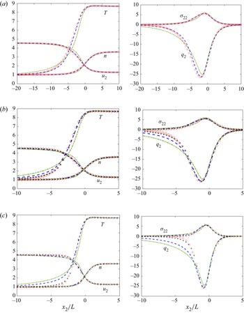
Figure 1 compares the shock wave structures obtained from the Boltzmann equation, the Shakhov model and the ESBGK model, when the upstream Mach number is  $5$. Different inverse power-law potentials, reflected through the viscosity index
 $\omega$ in (2.11), are considered. The Boltzmann equation is solved by the fast spectral method (Wu et al. Reference Wu, White, Scanlon, Reese and Zhang2013). For the Maxwellian gas with
 $\omega =1$, it is found that the Shakhov model gives a very good prediction of the shock structure, while the ESBGK model overpredicts the temperature and heat flux in the upstream part. When the viscosity index decreases to 0.75 and eventually to 0.5 of the HS gas, the Shakhov model still predicts the density and velocity profiles well but significantly overpredicts the temperature and heat flux in the upstream part: the smaller the value of
 $\omega$, the larger the deviation. For the ESBGK model, the deviations of temperature and heat flux from those of the Boltzmann equation are large for all values of
 $\omega$, and similarly the overprediction of the upstream temperature and heat flux can be clearly observed. The better performance of the Shakhov model over the ESBGK model suggests the importance of including the heat flux in the gain term of the modelled collision operator (3.9).
The Mach 5 shock wave structures for molecules interacting through inverse power-law potentials: Shakhov model, blue dashed line; ESBGK model, green dash-dotted lines; Boltzmann equation, red circles;  $\nu$-model, Asterisks. Note that the characteristic length is chosen to be the mean free path
 $L=({16}/{5{\rm \pi} })\sqrt {{{\rm \pi} }/{2mk_BT_0}} ({\mu (T_0)}/{n_0})$ in the upstream part of the normal shock wave, so we take
 $Kn=5{\rm \pi} /16$ in the numerical simulation. The shock density centre is at
 $x_2=0$. (a) Maxwell gas,
 $\omega =1$; (b) inverse power-law potential,
 $\omega =0.75$; and (c) HS gas,
 $\omega =0.5$.

To determine the velocity-dependent collision frequency  $\nu (\xi )$ in the
 $\nu$-model, we first use the equilibrium collision frequency
 $\nu _{eq}(\xi )$ defined in (2.17) and (2.20) with the normalisation (3.13), and find that the upstream temperature is underestimated (not shown). Therefore, a flatter collision frequency curve is required; after a few trial-and-errors we find that good agreement in the shock structures can be achieved (see figure 1) when the following semiempirical formula is used:
 \begin{equation} \nu_\omega(\xi)=A\frac{p}{\mu}[\nu^{0}_{eq}(\xi)+2\nu^{0}_{eq}(0)], \end{equation}
where  $A$ is determined from (3.13). Note that the velocity-independent parameter
 $\nu _\eta ^{0}$ in (2.17) is automatically eliminated after the normalisation (3.13) so we directly use
 $\nu ^{0}_{eq}$ in (5.1).
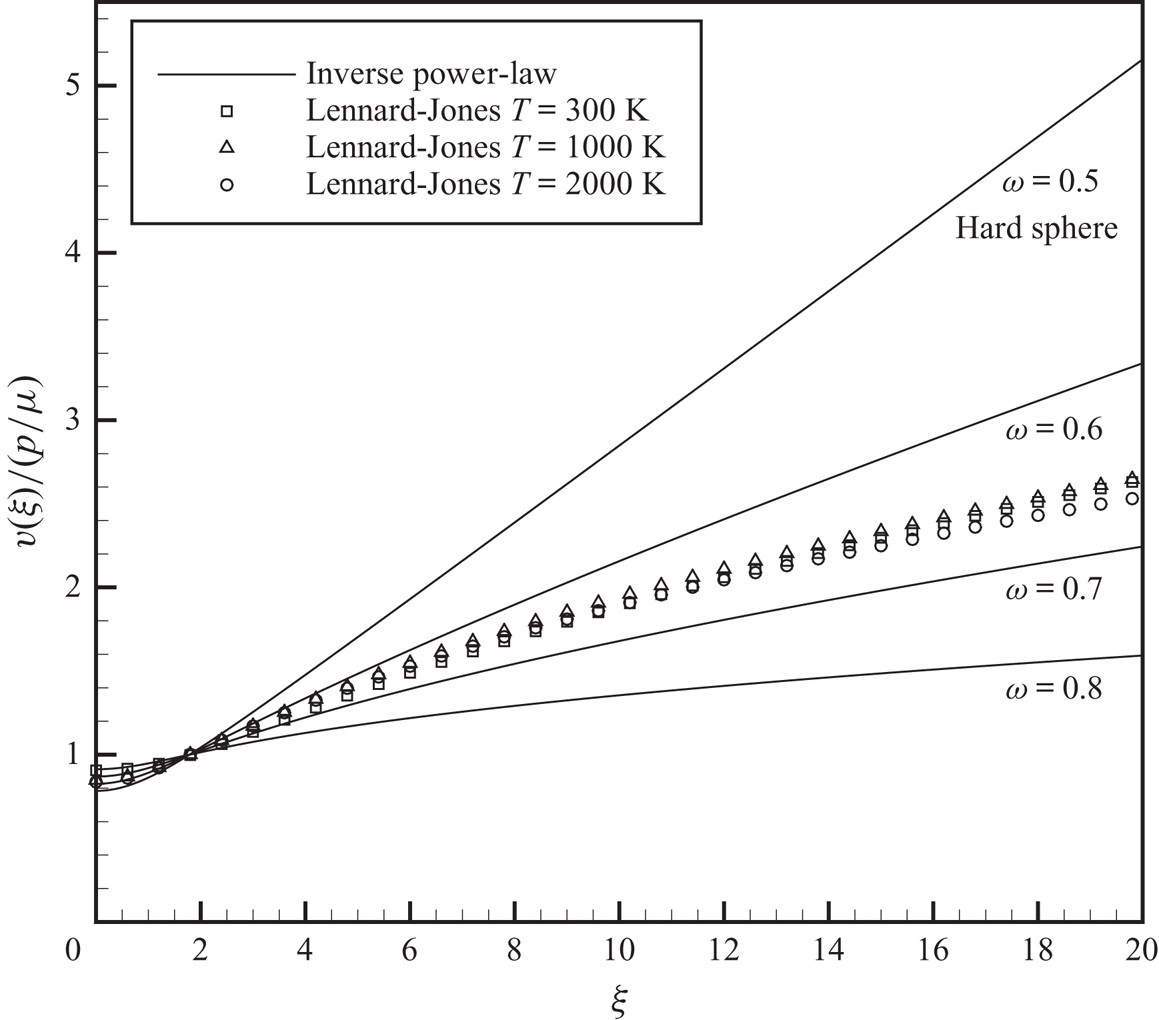
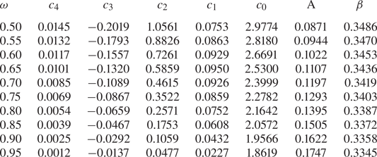
The collision frequency (5.1) for typical inverse power-law potential is shown in figure 2. In numerical simulations,  $\nu ^{0}_{eq}(\xi )$ can be calculated by fitting functions and the parameters for typical values of viscosity index are summarised in table 1. The term
 $2\nu ^{0}_{eq}(0)$ is an empirical parameter, which makes the collision frequency curve flatter and accounts for the deviation of collision frequency in non-equilibrium state from that in the Maxwellian distribution. The semiempirical formula (5.1) is implemented in all of the test cases performed in this paper. It will be demonstrated that this semiempirical formula works well not only in normal shock waves, but also in other test cases and has a certain degree of universality. It is also worth noting that for Maxwellian molecules the collision frequency
 $\nu (\xi )$ is velocity-independent, so the
 $\nu$-model reduces to the Shakhov model.


Numerical fitting of the equilibrium collision frequency by the quartic function  $\nu ^{0}_{eq}(\xi )=\sum _{j=0}^{4}c_j\xi ^{j}$, when
 $\xi \le 5$, as well as the constants
 $A$ in (3.13) and
 $\beta$ in (3.14). When
 $\xi >5$, the collision frequency
 $\nu ^{0}_{eq}$ can be approximated when the first-order Taylor expansion is applied to (2.17), resulting in
 $\nu ^{0}_{eq}= (2-\omega )\sqrt {{\rm \pi} }\xi ^{2(1-\omega )}$. In the calculation of
 $\beta$ we take the Prandtl number to be
 ${Pr}=2/3$, while the collision frequency is given by (5.1).

5.1.2. Lennard-Jones potential
The  $\nu$-model for the Lennard-Jones potential can be proposed straightforwardly, where the velocity-dependent collision frequency is designed to be a linear combination of those based on the inverse power-law potentials, in accordance with (2.12),
 \begin{equation} \nu_{LJ}(v)=A_{LJ}\sum_{j=1}^{3}b_j\left(\frac{k_BT}{\epsilon} \right)^{0.5-\omega_j}\times\nu_{\omega_j}(\xi), \end{equation}
and  $A_{LJ}$ can be determined from (3.13). Figure 2 shows the typical collision frequency curves calculated by (5.2) for the Lennard-Jones potential. Unlike the inverse power-law potential, the shape of the collision frequency curve is different at different temperatures for the Lennard-Jones potential.
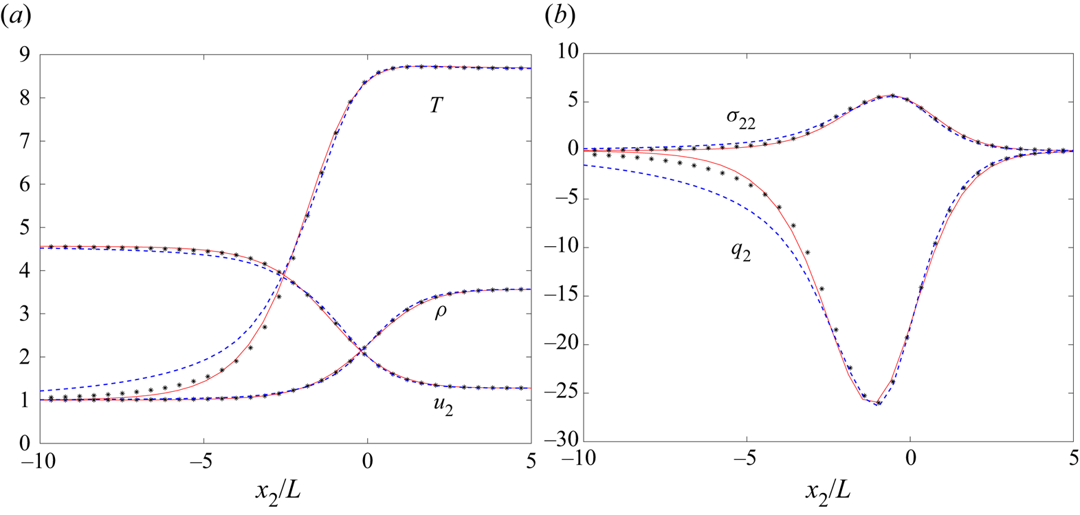
For the normal shock wave with Mach number 5 and upstream temperature  $T_0=300$ K, the downstream temperature is 2604 K. For argon with potential depth
 $\epsilon =119.2k_B$ in (2.6), the viscosity given by (2.9) and (2.12) works well when the temperature is between 100 and 3000 K. Figure 3 shows the macroscopic variable distributions along the flow direction calculated by different kinetic models. It is seen that the
 $\nu$-model yields consistent results with those from the Boltzmann equation, while the Shakhov model significantly overpredicts the temperature and heat flux in the upstream area. Note that Wu et al. (Reference Wu, White, Scanlon, Reese and Zhang2013) have shown that the density, velocity and temperature from the Boltzmann equation with the collision kernel (4.5) agree with those from the molecular dynamics simulations of Valentini & Schwartzentruber (Reference Valentini and Schwartzentruber2009).


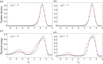
To further assess the accuracy of different kinetic models, figure 4 compares the marginal velocity distributions, especially the thermal energy distribution
 \begin{equation} F_{{thermal}}=\iint_{-\infty}^{\infty} {c^{2}f}\, {{\rm d}}v_1 \, {{\rm d}}v_3, \end{equation}
at the upstream locations  $x_2/L=-5$ and
 $-7$, where the deviations in temperature and heat flux are large. It can be found that the number density distributions are nearly the same for different collision models, while the thermal energy distributions exhibit large discrepancy. The latter is analysed as follows. At
 $x_2/L=-5$ and
 $-7$, comparing with the Boltzmann solution, an extra bump around
 $v_2=-3$ for the thermal energy curve of the
 $\nu$-model and Shakhov model is observed. This energy peak soon diminishes going upstream in the
 $\nu$-model, while in the Shakhov model there still exists an obvious energy peak even at the very upstream location
 $x_2/L= -7$. This suggests that, in the Shakhov model, molecules with large negative velocities arising from the high temperature postshock gas can travel a very long distance from downstream to upstream, which significantly heats the gas therein. This is why the Shakhov model (and also for the ESBGK model) overpredicts the temperature and heat flux in the upstream.
Marginal VDFs in the argon normal shock wave of  ${Ma}=5$, using the Lennard-Jones potential. (a,b) Number density distribution
 $\int {f}\, {\textrm {d}}v_1\, {\textrm {d}}v_3$ and (c,d) thermal energy distribution
 $\int {c^{2}f}\, {\textrm {d}}v_1\, {\textrm {d}}v_3$. Solid lines, Boltzmann solutions; asterisks,
 $\nu$-model with the collision frequency (5.2); blue dashed lines, Shakhov model.

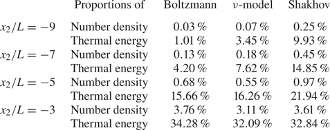
Table 2 further quantifies the number density and thermal energy occupied by molecules with  $v_2<0$. Although the number of molecules with
 $v_2<0$ are small (less than 3.76 %), they carry quite a part of the energy (up to 34.28 %). In the upstream region
 $x_2/L<-5$, the proportion of thermal energy carried by molecules with
 $v_2<0$, predicted by the Shakhov model, is much larger than those of the
 $\nu$-model and Boltzmann equation.
Proportions of the molecular number density  $\int _{{v_2} < 0} {f\, {\textrm {d}}\boldsymbol v}/\int {f\, {\textrm {d}}\boldsymbol v}$ and thermal energy
 $\int _{{v_2} < 0} {c^{2}f\, {\textrm {d}}\boldsymbol v} /\int {c^{2}f\, {\textrm {d}}\boldsymbol v}$ occupied by molecules with
 $v_2<0$, in the argon normal shock wave with
 ${Ma}=5$.

Based on the above analysis, in order to fix the overprediction of temperature and heat flux on top of the Shakhov model, the collision frequency of molecules with large speed should be increased to prevent high-speed molecules travelling too far to the upstream. Therefore, in our  $\nu$-model, we design the velocity-dependent collision frequency based on the equilibrium collision frequency (2.17), where high-speed molecules have higher collision frequency (figure 2), which effectively suppresses the heating of upstream gas due to the high speed
 $v_2<0$ molecules from the shock downstream.
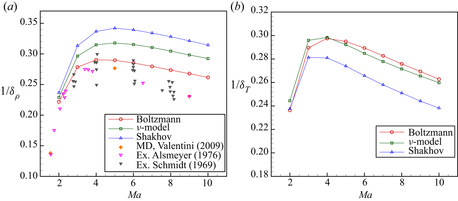
At the end of this subsection, to show that our  $\nu$-model works for other values of Mach number, the reciprocal shock thickness is calculated by different kinetic equations in a wide range of Mach number, as shown in figure 5. The discrepancy between the Boltzmann solution and the experimental results in
 $Ma >6$ is because the approximation (2.12) for the Lennard-Jones potential is only applicable between 100 and 3000 K (Wu et al. Reference Wu, White, Scanlon, Reese and Zhang2013). Here we mainly focus on the difference between the Boltzmann solution and the results of kinetic models. For the density-based thickness, the deviation between the results of the Shakhov model and the Boltzmann solution is around
 $7\,\%$–
 $20\,\%$. However, the deviation of the results predicted by the
 $\nu$-model is much smaller. For the temperature-based thickness, the results of the
 $\nu$-model are quite consistent with the Boltzmann solution in a wide range of Mach number, with a maximum deviation around 3 %. The Shakhov model, however, predicts significantly thicker shock waves in the large Mach number. This shows the
 $\nu$-model can yield more accurate temperature distribution than the Shakhov model in the large Mach number.
Reciprocal shock thickness in argon normal shock wave.  $\delta _\rho =({{{\rho _1} - {\rho _0}}})/{{\max ({\textrm {d}}\rho /{\textrm {d} x})}}$ and
 $\delta _T=({{{T _1} - {T _0}}})/{{\max ({\textrm {d}}T /{\textrm {d} x})}}$, where
 $\rho _0,T_0$ and
 $\rho _1,T_1$ are the upstream and downstream quantities, respectively. Results of molecular dynamics (MD) simulations are adopted from Valentini & Schwartzentruber (Reference Valentini and Schwartzentruber2009). Experimental results are adopted from Alsmeyer (Reference Alsmeyer1976) and Schmidt (Reference Schmidt1969). (a) Density-based thickness and (b) temperature-based thickness.

5.2. Space-homogeneous relaxation of bimodal distribution function
A space-homogeneous relaxation is further performed to investigate the evolution of bimodal VDF (typical in shock waves) as well as high-order moments. The initial distribution function is set as a blend of two different Maxwellian distributions, and with the normalisation (4.1) the initial VDF has the form
 \begin{align} f &= \frac{1}{{13}}{\left( {\frac{2}{{\rm \pi} }} \right)^{3/2}}{\exp\{{ - 2[ {{{({v_x} - 3)}^{2}} + v_y^{2} + v_z^{2}} ]}\}} \nonumber\\ &\quad + \frac{{12}}{{13}}{\left( {\frac{2}{{\rm \pi} }} \right)^{3/2}}{\exp\left\{ - 2\left[ {{{\left({v_x} + \frac{1}{4}\right)}^{2}} + v_y^{2} + v_z^{2}} \right]\right\}}, \end{align}
which corresponds to the macroscopic state  $n=1$,
 $\boldsymbol {u}=\boldsymbol {0}$ and
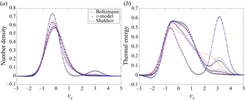
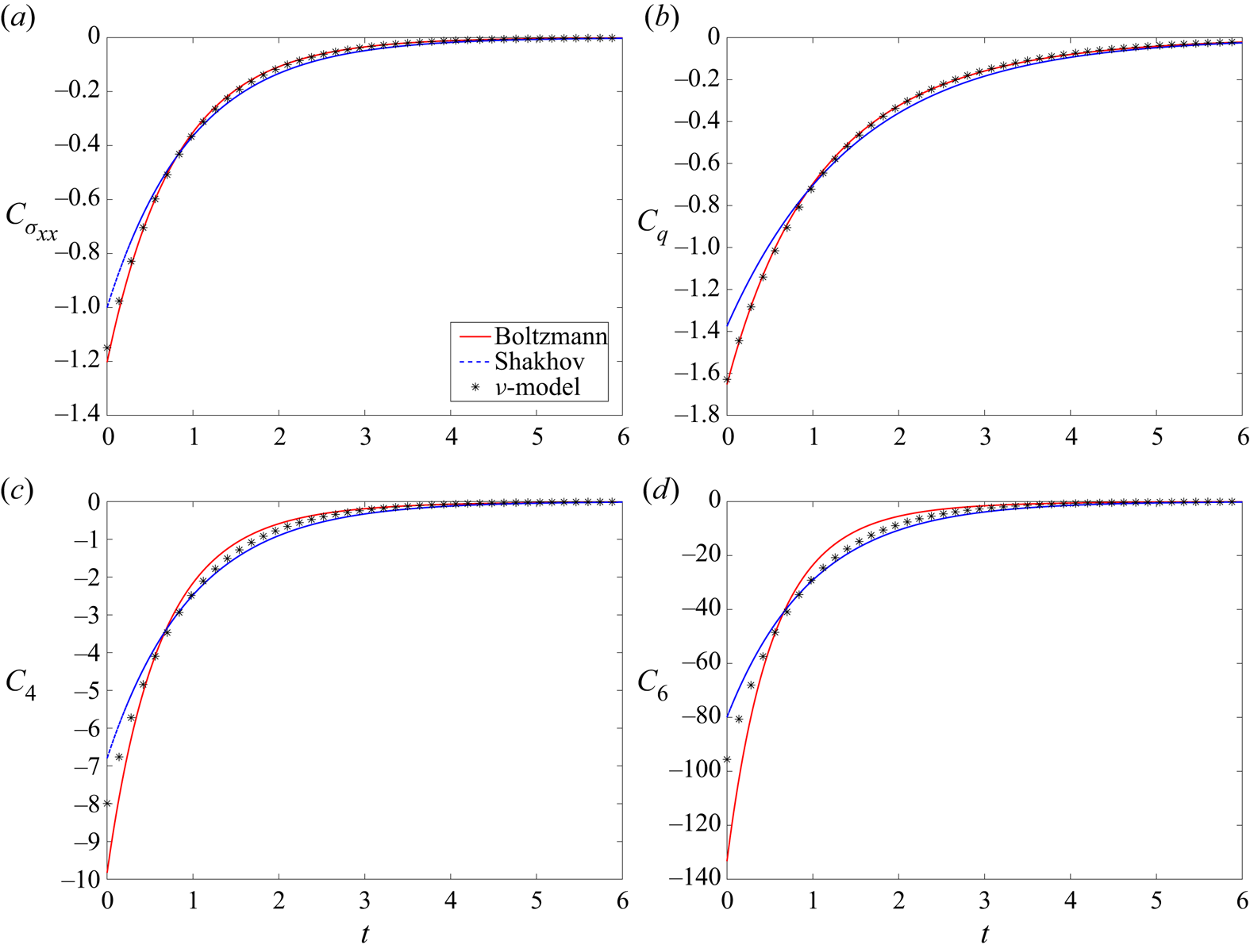
 $T=1$. As shown in figure 4, such a bimodal distribution characterises the VDF in front of the shock wave where strong non-equilibrium effects exist. The Lennard-Jones potential is used. The time evolutions of the distribution function and the collision integrals obtained by different kinetic models are compared with the Boltzmann solution in figures 6 and 7. It is shown that both kinetic models cannot completely recover the relaxation behaviour of the Boltzmann operator. Nevertheless, as shown in figure 7, the collision integrals for different moments obtained from the
 $\nu$-model are more accurate than those from the Shakhov model, especially for collision integrals about the viscous stress and the heat flux where the
 $\nu$-model agrees perfectly well with the Boltzmann equation. This improvement is because, as shown in figure 6, the
 $\nu$-model has relatively faster relaxation of high-speed molecules than that of the Shakhov model, and hence faster (more accurate) relaxation of the moments.
Space-homogeneous relaxation of bimodal distribution function. Evolution of (a) the reduced number density distribution  $\int f \, {\textrm {d}}v_y\, {\textrm {d}}v_z$ and (b) the thermal energy distribution
 $\int \boldsymbol {c}^{2}f \, {\textrm {d}}v_y\, {\textrm {d}}v_z$. The time, normalised by
 $\mu /p$, corresponding to each line (in the direction towards Maxwellian distribution) is
 $t=0, 1.2, 2.4, 3.6$.

Evolution of the collision integrals for different moments in the space-homogeneous relaxation of bimodal distribution function: (a)  $C_{\sigma _{xx}}=2\int (c_x^{2}-|\boldsymbol {c}|^{2}/3)Q \, {\textrm {d}} \boldsymbol {v}$; (b)
 $C_{q}=\int c_x|\boldsymbol {c}|^{2}Q \, {\textrm {d}} \boldsymbol {v}$; (c)
 $C_{4}=\int c_x^{4}Q \, {\textrm {d}} \boldsymbol {v}$; (d)
 $C_{6}=\int c_x^{6}Q \, {\textrm {d}} \boldsymbol {v}$. The time
 $t$ is normalised by
 $\mu /p$.

5.3. Supersonic flow around a circular cylinder
The supersonic flow around a circular cylinder is simulated to further assess the performance of our  $\nu$-model. The inverse power-law potentials with
 $\omega =0.81$ and
 $\omega =0.5$ are implemented. It is demonstrated that the results of
 $\omega =0.81$ from the
 $\nu$-model share a similar accuracy with those of
 $\omega =0.5$, so only the results of
 $\omega =0.5$ (the HS gas) are shown here to save space. Four free stream conditions,
 $Ma =5,20$ and
 ${Kn}_{{HS}}=0.1,1$ are considered, where the Knudsen number
 ${Kn}_{{HS}}$ is defined by the cylinder radius
 $r$ and the mean free path
 $L_{{HS}}$ of the HS model, i.e.
 \begin{equation} {L_{{{HS}}}} = \frac{16}{5}\frac{\mu(T_\infty) }{{\rho \sqrt {2{\rm \pi} RT_\infty} }}. \end{equation}
The full diffuse reflection condition is imposed on the cylinder surface and the wall temperature is fixed at the free stream temperature:  $T_{{w}}=T_{\infty }$. For the discretisation of physical space, a structured mesh in polar coordinates is used. The mesh size in the normal direction is refined approaching the cylinder surface, with the minimum mesh height set as
 $0.004r$ for
 $Ma =5$ and
 $0.0006r$ for
 $Ma =20$ to ensure the grid independence of surface stress and heat flux. Due to the multiscale and implicit nature of our numerical scheme, the computational cost is kept small. For the discretisation of velocity space,
 $90 \times 90 \times 50$ uniform points in the velocity range
 $[-15a_{\infty },15a_{\infty }]$ and
 $160 \times 160 \times 128$ uniform points in the velocity range
 $[-55a_{\infty },55a_{\infty }]$ are adopted for
 $Ma =5$ and
 $Ma =20$, respectively, where
 $a_{\infty }$ is the free stream acoustic velocity.
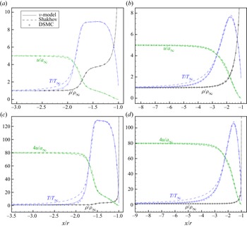
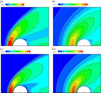
Numerical results of the flow variable distributions along the central horizontal line are shown in figure 8. It is seen that the  $\nu$-model predicts quite satisfactory results consistent with the DSMC results calculated by the DS2V code (Bird Reference Bird2005). For the Shakhov model, the accuracy in velocity profiles deteriorates slightly, and the upstream temperature is significantly overpredicted. Figure 9 shows that the temperature distributions around the cylinder obtained from the
 $\nu$-model agree well with the DSMC results, while the Shakhov model exhibits large deviation, especially in the upstream of bow shock.
Density, velocity and temperature variables along the central horizontal line in the front of cylinder, in supersonic flows of HS gas around a circular cylinder: (a)  $Ma =5$,
 ${Kn}_{{HS}}=0.1$; (b)
 $Ma =5$,
 ${Kn}_{{HS}}=1$; (c)
 $Ma =20$,
 ${Kn}_{{HS}}=0.1$; (d)
 $Ma =20$,
 ${Kn}_{{HS}}=1$.

Temperature contours in supersonic flows of HS gas around a circular cylinder. Colour bands,  $\nu$-model; black dashed lines, Shakhov model; black solid lines, DSMC results. Here (a)
 $Ma =5$,
 ${Kn}_{{HS}}=0.1$; (b)
 $Ma =5$,
 ${Kn}_{{HS}}=1$; (c)
 $Ma =20$,
 ${Kn}_{{HS}}=0.1$; (d)
 $Ma =20$,
 ${Kn}_{{HS}}=1$.

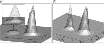
To further investigate the mechanism of such an improvement of the  $\nu$-model for temperature prediction, the thermal energy distributions in the upstream of the bow shock for
 $Ma =5$ are shown in figure 10. For this set of figures we sum up the following notable points.
(i) Molecules with
 $v_x<0$ form an obvious energy peak, especially in the case of ${Kn}_{{HS}}=1$. As a supplement to the data shown in figure 10 when $Ma =5$, at $Ma =20$ in the temperature early-rising region, the Shakhov model predicts the proportions of thermal energy occupied by molecules with $v_x<0$ to be 42.03 % when ${Kn}_{{HS}}=0.1$ and 61.62 % when ${Kn}_{{HS}}=1$, while in the $\nu$-model these data are 9.38 % and 37.18 %, respectively. This suggests that the high speed (large peculiar velocity) $v_x<0$ molecules arising from the postshock gas have a big impact on the thermal energy of the upstream preshock gas and cause a significant heating.
(ii) The thermal energy peak due to the high speed
$v_x<0$ molecules predicted by the $\nu$-model is much lower than that predicted by the Shakhov model. This is because that in the $\nu$-model the velocity-dependent collision frequency (5.1) is adopted, where the molecule with larger peculiar velocity has higher collision frequency; and intensive collisions prevent them from transporting upstream too far, and thus the overprediction of upstream temperature observed in the Shakhov model is suppressed in the $\nu$-model. This also suggests that, when the viscosity index $\omega$ approaches $0.5$ and when the Mach number gets larger, temperature overprediction by the Shakhov model will become more severe due to the steeper collision frequency curve (figure 2) and higher peculiar velocity of $v_x<0$ molecules.


Thermal energy distributions  $\int {c^{2}f\, {\textrm {d}} {v_z}}$ in supersonic flows of HS gas of
 $Ma =5$ around a circular cylinder, at locations before the bow shock: (a)
 ${Kn}_{{HS}}=0.1$ at
 $(x,y)=(-2.2r,-0.055r)$, molecules with
 $v_x<0$ occupy 15.38 % and 5.65 % of the total thermal energy in the Shakhov model and
 $\nu$-model, respectively; (b)
 ${Kn}_{{HS}}=1$ at
 $(x,y)=(-4.4r,-0.11r)$, molecules with
 $v_x<0$ occupy 23.63 % and 14.70 % of the total thermal energy in the Shakhov model and
 $\nu$-model, respectively. Grey surface,
 $\nu$-model; wire frame, Shakhov model.

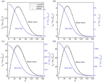
Distributions of the shear stress and heat flux on the cylinder surface are shown in figure 11. When  ${Ma }=5$, the
 $\nu$-model and the Shakhov model predict almost the same results and they both agree well with DSMC. This is because for the high-temperature postshock gas, there are few molecules with large peculiar velocity and the collision frequency in the Shakhov model is comparable to that in the
 $\nu$-model. When
 ${Ma }=20$, a certain degree of discrepancy exists between the results of the Shakhov and
 $\nu$-models, and the
 $\nu$-model shows better agreement with DSMC. The drag coefficient
 $C_d$ and heat transfer coefficient
 $C_h$ for the cylinder at
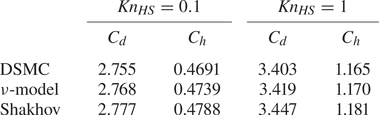
 ${Ma }=20$ are further shown in table 3, where it can be found that the
 $\nu$-model predicts slightly more consistent results than the Shakhov model, although in general the difference among the three sets of results is small.
Distributions of the shear stress and heat flux along the cylinder surface, in supersonic flows of HS gas around a circular cylinder: (a)  $Ma =5$,
 ${Kn}_{{HS}}=0.1$; (b)
 $Ma =5$,
 ${Kn}_{{HS}}=1$; (c)
 $Ma =20$,
 ${Kn}_{{HS}}=0.1$; (d)
 $Ma =20$,
 ${Kn}_{{HS}}=1$.

Drag coefficient  $C_d$ and heat transfer coefficient
 $C_h$ in supersonic flows of HS gas of
 ${Ma }=20$ around a circular cylinder. Here
 $C_d=D/(\frac {1}{2}\rho _\infty \boldsymbol {u}_\infty ^{2}r)$,
 $C_h=H/(\frac {1}{2}\rho _\infty \boldsymbol {u}_\infty ^{3}r)$, where
 $D$ and
 $H$ are the total stress and the total heat flux on the cylinder surface, respectively. The numerical errors for the results of kinetic models are estimated as 0.2 % for
 $C_d$ and 0.45 % for
 $C_h$.

6. Numerical results in microflows
In this section we assess the accuracy of the  $\nu$-model in canonical rarefied microflows, with the velocity-dependent collision frequency determined from the strong normal shock waves.
6.1. Planar Couette flow
Unlike the normal shock wave that is dominated by the effects of compressibility, the Couette flow is shear dominated. It is a typical rarefied gas flow since the heat flux parallel to the plates is not zero, in sharp contrast to the Navier–Stokes–Fourier equations. Here we consider the Couette flow between two parallel plates with temperature  $T_0$, where the wall speed is equal to the most probable speed of gas molecules at
 $T_0$, i.e.
 $Ma =\sqrt {1.2}$. The case of a much lower Mach number
 $Ma =0.1\sqrt {1.2}$ has also been performed and the comparison of results from different kinetic models is similar to the case shown here. For simplicity we only consider the Maxwellian and HS gases, since for other gases with viscosity index
 $0.5\le \omega \le 1$, the results fall between those of Maxwellian and HS gases. The characteristic flow length
 $L$ in (4.4) is chosen to be the distance between the two plates.
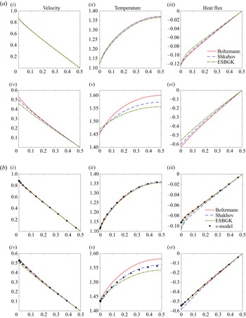
For the Maxwellian gas, when  ${Kn}=0.1$, figure 12(a) shows that the Shakhov model produces close results to those of the Boltzmann equation, while the ESBGK model has slight errors in temperature and heat flux. When
 $Kn=1$, the difference between the Shakhov/ESBGK model and the Boltzmann equation increases, but we see that the Shakhov model is better than the ESBGK model, in velocity, temperature and heat flux. However, when the HS gas is considered, figure 12(b) shows that the Shakhov model is better than the ESBGK model in terms of temperature, but is worse in heat flux.
Couette flow: panels (i–iii),  $Kn=0.1$; panels (iv–vi),
 $Kn=1$. The abscissas
 $x_2$ are for the spatial coordinate, which is in the direction perpendicular to the two plates and normalised by the wall distance. The two plates are located in
 $x_2=0$ and
 $x_2=1$. Variables are under the normalisation of (4.1). The heat flux is parallel to the wall velocity. Due to symmetry, only the half-spatial region is shown. (a) Maxwell gas and (b) HS gas.

When the  $\nu$-model is used, we find that its heat flux agrees well with the solution of the Boltzmann equation. However, there is no improvement in the temperature profile as compared with the Shakhov model; nevertheless, the relative error in temperature to that of the Boltzmann equation is within 3 %. It is also worth noting that the
 $\nu$-BGK and
 $\nu$-ESBGK models (Mieussens & Struchtrup Reference Mieussens and Struchtrup2004; Zheng & Struchtrup Reference Zheng and Struchtrup2005) predict even worse results than the standard ESBGK, and they are not suggested for Couette flow (Zheng & Struchtrup Reference Zheng and Struchtrup2005).
6.2. Thermal transpiration
Another typical phenomenon in rarefied gas dynamics is thermal transpiration, where the gas moves towards a hotter region even in the absence of a pressure gradient (Maxwell Reference Maxwell1879; Reynolds Reference Reynolds1879). Harnessing this unique property leads to the design of the Knudsen compressor that pumps the gas without any moving mechanical parts (Vargo et al. Reference Vargo, Muntz, Shiflett and Tang1999; Gupta & Gianchandani Reference Gupta and Gianchandani2008). This problem is a good test case since even when the value of viscosity is the same, different intermolecular potentials yield a different thermal slip velocity (Wang, Su & Wu Reference Wang, Su and Wu2020) and mass flow rate (Sharipov & Bertoldo Reference Sharipov and Bertoldo2009; Wu et al. Reference Wu, Liu, Zhang and Reese2015a); and this can be captured neither by the relaxation model (1.1) with velocity-independent collision frequency, nor by the Fokker–Planck model.
Here we assess the performance of our  $\nu$-model in thermal transpiration between two parallel plates and focus on the steady-state solutions. The governing equation reads
 \begin{equation} v_2\frac{\partial {f}}{\partial{x_2}}=Q+{\rm{source}}, \end{equation}
where the source term is  $-a_0v_1(c^{2}-5/2)F_{eq}$, with
 $a_0$ being a small constant related to the temperature gradient along the solid wall. The induced flow velocity due to rarefaction effects is proportional to
 $a_0$, and the final result will be further normalised by
 $a_0$.
Figure 13 shows the induced velocity for Maxwell and HS gases. Numerical solutions of the Boltzmann equation with different values of the viscosity index  $\omega$ are different. However, the viscosity index does not affect the solution in the Shakhov and ESBGK models. This is because the gas temperature does not change in the direction perpendicular to the solid wall, so that the coefficient in the collision operator (4.6) has nothing to do with the viscosity index
 $\omega$. That is,
 \begin{equation} \frac{\sqrt{\rm \pi}}{2Kn}\times\frac{\mu(T_0)}{n_0k_BT_0}\times\nu \left(\frac{c}{T}\right)=\frac{\sqrt{\rm \pi}}{2Kn}. \end{equation}
Thus, the Shakhov and ESBGK models with molecular-velocity-independent collision frequency do not have the degree of freedom to describe the change of intermolecular potential, while for the  $\nu$-model the intermolecular potential has an impact on the velocity-dependent collision frequency (5.1) and it predicts different results.
Velocity profiles in the thermal transpiration between two parallel plates. Abscissas are for the spatial coordinate  $x_2$ which is perpendicular to the two plates and normalised by the wall distance. The two plates are located in
 $x_2=0$ and 1. Due to symmetry, only half-spatial region is shown. Note that the Shakhov and ESBGK models do not distinguish the influence of intermolecular potential, and the
 $\nu$-model is reduced to the Shakhov model for Maxwellian gas. Here (a)
 $Kn=0.01$; (b)
 $Kn=0.1$; (c)
 $Kn=1$.

When  $Kn=0.01$, it is seen from figure 13(a) that the Shakhov model well predicts the velocity profile of the Maxwell gas (i.e. the thermal slip velocity and the Knudsen layer function are all captured (Wang et al. Reference Wang, Su and Wu2020)), while the ESBGK model predicts a slight low velocity. However, both kinetic models cannot predict the velocity profile of HS gas. This problem is fixed in the
 $\nu$-model. When the Knudsen number is increased to 0.1, the Shakhov and ESBGK models predict a close velocity profile to that of the Maxwell and HS gas, respectively. When the
 $\nu$-model is used, good agreement with the Boltzmann equation solution is observed. When the Knudsen number further increases, the
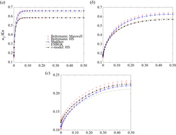
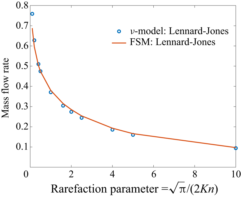
 $\nu$-model always predicts better velocity profiles than the Shakhov and ESBGK models. We also solve the thermal transpiration using the Lennard-Jones potential. The fast spectral solution is obtained from Wu et al. (Reference Wu, Liu, Zhang and Reese2015a), while the
 $\nu$-model uses the collision frequency (5.2). It can be seen in figure 14 that the
 $\nu$-model has good accuracy for the Knudsen number up to approximately unity.
Mass flow rate  $2\int _0^{1} {{u_1}\, {\textrm {d}} {x_2}}$ versus the rarefaction parameter in the thermal transpiration of argon when the Lennard-Jones potential is used. The wall temperature is 300 K. The reference result is the Boltzmann solution calculated by the fast spectral method (FSM).

From this test case we can clearly see that there are more degrees of freedom in the  $\nu$-model to recover more details of the intermolecular collision, and thus yield more accurate results than the standard Shakhov and ESBGK models with velocity-independent collision frequency.
6.3. Thermal transpiration in cavity
We further investigate the thermal transpiration of an HS gas in a two-dimensional cavity with a length-to-width ratio of 5. The temperature at the right-hand wall is set to be twice that of the left-hand wall, while the temperature of the top and bottom walls varies linearly along the channel. The Knudsen number  $Kn$ is defined at the average temperature of the left-hand and right-hand walls, the average molecular number density
 $n$, and the cavity height
 ${L}$. Due to symmetry, only the half-spatial region
 $0\le y\le {L}/2$ is considered.
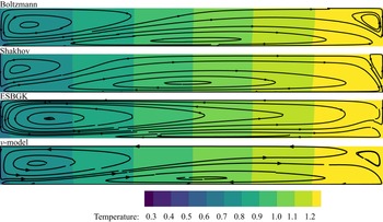
The temperature fields and the streamlines obtained from the Boltzmann equation, Shakhov model, ESBGK model and  $\nu$-model are compared in figure 15, when
 $Kn=0.5$. All kinetic models predict a good temperature field with the Boltzmann solution, but not for velocity. For the Boltzmann solution the flow is characterised by three vortexes: the left-hand vortex, the bottom vortex and the right-hand vortex adjoining the left-hand wall, the bottom wall and the right-hand wall, respectively. For the Shakhov and ESBGK models their streamlines deviate largely from the Boltzmann solution in a different trend. The Shakhov model predicts a larger bottom vortex but smaller right-hand and left-hand vortexes, while the ESBGK model predicts a much larger left-hand vortex with a significantly shrunken bottom vortex and the right-hand vortex completely disappears. By contrast, the
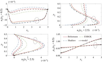
 $\nu$-model predicts nearly the same flow pattern with the Boltzmann solution. The velocity and normal stress profiles are further shown in figure 16, when
 $Kn=0.1$ and
 $0.5$. The profiles coincide with the above observations about the flow field data that all kinetic models predict similar normal stress profiles agreeing well with the Boltzmann solution, but quite different velocity profiles where only those from the
 $\nu$-model show good agreement with the Boltzmann solution at different
 $Kn$ numbers.
Thermal transpiration of HS gas in a rectangular cavity of aspect ratio 5: temperature fields and streamlines (in half of the channel) calculated by Boltzmann equation and different kinetic models. The Knudsen number is 0.5.

Thermal transpiration of HS gas in a rectangular cavity: velocity and normal stress profiles calculated by Boltzmann equation and different kinetic models. The cavity aspect ratio is 5, Knudsen numbers are 0.1 (results passing through circles) and 0.5, respectively.

7. The computational efficiency
As previously stated, the main motivation for constructing a kinetic model is to reduce the computational cost while imitating as closely as possible the behaviour of the Boltzmann equation. This means that for any kinetic model there must be a trade-off between accuracy and efficiency. In previous sections, the improved accuracy of the  $\nu$-model has been demonstrated and here the efficiency of the
 $\nu$-model will be investigated through benchmark cases.
The multiscale implicit scheme described in Appendix A is used to do the numerical simulations, with the  $\nu$-model and the Shakhov model applied, respectively. The convergence criterion for the numerical tests is that the global root mean square residuals are less than
 $10^{-9}$, where the residual vector is defined as (see (A11) for definitions of the variables)
 \begin{equation} {\boldsymbol{R}_i} ={-} {\frac{1}{{{V_i}}}\sum_{j \in N(i)} {{A_{ij}}{\boldsymbol{\mathcal{F}}}_{ij}} } . \end{equation}
In all the tests argon gas is assumed and the inverse power-law potential with viscosity index  $\omega =0.81$ is applied.
The first benchmark case is the lid-driven cavity flow. Three conditions including  ${{Re}}=1000$ and
 $Kn=0.1, 10$ are considered and the Mach number is around
 $0.16$. The computational time required to reach convergence is shown in table 4. The second benchmark case is Mach 5 flow around a circular cylinder. Two conditions,
 $Kn=0.1$ and 1 (based on the radius of the cylinder) are considered. The computational time is shown in table 5. It can be found that in different test cases the additional computational cost for the
 $\nu$-model relative to the Shakhov model ranges from 12.3 % to 21.2 %. Considering the significant accuracy improvement of the
 $\nu$-model detailed in the previous sections, an extra computation cost of 20 % is acceptable.
Computational time of the multiscale implicit scheme (see the Appendix A) to reach the residual  $10^{-9}$ for the lid-driven cavity flow simulation. The spatial mesh is
 $61\times 61$. Computation is executed on a single core of the computer with Intel(R) Xeon(R) Gold 6148 CPU @ 2.40 GHz.

Computational time of the multiscale implicit scheme (see the Appendix A) to reach the residual  $10^{-9}$ for the Mach 5 flow around a circular cylinder. The spatial mesh is
 $50\times 128$ and the velocity space is discretised as
 $90\times 90\times 50$. Parallel computing is used for these calculations on 40 cores of a computer with Intel(R) Xeon(R) Gold 6148 CPU @ 2.40 GHz.

We would like to also mention about the DSMC method which is widely employed in the rarefied flow simulation. The current kinetic model combined with the multiscale numerical scheme described in Appendix A mainly has two advantages over the DSMC method.
(i) The present method is a deterministic method and can efficiently yield smooth results for low-speed microflow. In contrast, as a stochastic simulation method, DSMC requires much more computing time to reduce the statistical noise to capture small variations of flow variables in the low-speed flow. As a reference, John, Gu & Emerson (Reference John, Gu and Emerson2011) have studied the cavity flow at
$Kn=10, 1, 0.075$ by DSMC, and the results have been obtained through intensive parallel computation on the supercomputer Blue Gene/P (BGP) with hundreds of processors. In the present study, the similar numerical results have been obtained by a single CPU core in a few hours, as shown in table 4.(ii) The present method applies to all flow regimes. While for DSMC, the cell size and time step are, respectively, limited by the mean free path and mean collision time, and the particle number per cell has some inherent constraints. This makes DSMC inapplicable to the continuum flow simulation. The case of cavity flow at
${Re}=1000$ shown in table 4 is unrealistic for DSMC.


On the other hand, DSMC shows superiority in the high-speed rarefied flow simulation, where the discretisation of the velocity phase space consumes plenty of memory for the deterministic discrete velocity method. Some comparisons about the accuracy and efficiency between the deterministic kinetic method and DSMC can be found in Huang, Xu & Yu (Reference Huang, Xu and Yu2012) and Zhu, Zhong & Xu (Reference Zhu, Zhong and Xu2017).
8. Conclusions
The  $\nu$-model has been developed to better approximate the BCO while keeping the computational cost at the same level as traditional gas kinetic models. The new model takes the relaxation-time approximation, where the target VDF to which the VDF relaxes is as simple as that in the Shakhov model, and the collision frequency is a function of the molecular velocity. A multiscale numerical method is used to solve the proposed model equation deterministically.
Based on the numerical simulation of normal shock waves, semiempirical formulae for the collision frequency are proposed for different intermolecular potentials, which showed certain universality for other rarefied gas flows. Specifically, in supersonic flows, the overprediction of temperature and heat flux in the upstream of shock wave caused by the heating of high-speed reflected molecules is suppressed or even eliminated; in thermal transpiration, the  $\nu$-model captures more derails of the intermolecular collision and predicts better results, while the Shakhov and ESBGK models with velocity-independent collision frequency cannot distinguish the influence of intermolecular potential.
In summary, the  $\nu$-model is able to recover more details of the intermolecular collision and predicts satisfactory results in a wide range of flow cases with various intermolecular potentials. In view of its good accuracy and easy implementation, we expect that it can be extended to better model rarefied flows of polyatomic gas and gas mixtures.
Funding
This work is supported by the National Natural Science Foundation of China under the grant number 12172162 and the Guangdong-Hong Kong-Macao Joint Laboratory for Data-Driven Fluid Mechanics and Engineering Applications in China under grant 2020B1212030001.
Declaration of interests
The authors report no conflict of interest.
Appendix A. Multiscale implicit scheme for steady state solution of the $\nu$-model

Discretising the physical space by the finite volume method, applying the implicit backward Euler formula for the time, and discretising the velocity space into discrete velocity points, the implicit discrete equation for the  $\nu$-model can be written as
 \begin{equation} \frac{{{V_i}}}{{{\rm \Delta} t}_i^{n+1}}( {f_{i,k}^{n + 1} - f_{i,k}^{n}} ) + \sum_{j \in N( i )} ({{A_{ij}}{\boldsymbol{v}_k} \boldsymbol{\cdot} {\boldsymbol{n}_{ij}}f_{ij,k}^{n + 1}}) = {V_i}\nu _{i,k}^{n + 1}( {f_{{r},i,k}^{n + 1} - f_{i,k}^{n + 1}} ), \end{equation}
where  $i,n,k$ correspond to the discretisation in physical space, time and velocity space, respectively;
 $j$ denotes the neighbouring cell of cell
 $i$ and
 $N( i )$ is the set of all of the neighbours of
 $i$;
 $ij$ denotes the variable at the interface between cell
 $i$ and
 $j$;
 $A_{ij}$ is the interface area,
 ${\boldsymbol {n}_{ij}}$ is the outward normal unit vector of interface
 $ij$ relative to cell
 $i$, and
 $V_i$ is the volume of cell
 $i$;
 ${{\rm \Delta} t}_i^{n+1}$ is the local time step and can be handled by various of traditional implicit time step control techniques.
Equation (A1) can be rearranged into incremental form as
 \begin{align} &\left( {\frac{{{V_i}}}{{{\rm \Delta} t}_i^{n+1}} + {V_i}\nu_{i,k}^{n+1}} \right){\rm \Delta} f_{i,k}^{n + 1} + \sum_{j \in N(i)} {{A_{ij}}{{\boldsymbol v}_k} \boldsymbol{\cdot} {{\boldsymbol n}_{ij}}{\rm \Delta} f_{ij,k}^{n + 1}} \nonumber\\ &\quad = {V_i}\nu_{i,k}^{n+1}({f_{{{r}},i,k}^{ n + 1} - f_{i,k}^{n}}) - \sum_{j \in N(i)} {{A_{ij}}{{\boldsymbol v}_k} \boldsymbol{\cdot} {{\boldsymbol n}_{ij}}f_{ij,k}^{n}}, \end{align}
where terms on the left-hand side of the equal sign are the increments and will converge to zero when the steady state is reached. In the following paragraphs, the terms on the right-hand side of (A2) are determined first, and then the increment of the distribution function  ${\rm \Delta} f_{i,k}^{n + 1}$ can be worked out to update the variables for one time step.
It is well known that the conventional discrete velocity method will suffer from excessive numerical viscosity and yield over-dissipating results in the case of small  $Kn$ number. To avoid this problem and ensure good accuracy both in the collisionless limit as well as the hydrodynamic limit, the calculation of the interface distribution function
 $f_{ij,k}^{n}$ should be carefully handled. Here, the construction of the interface distribution function proposed by Yuan & Zhong (Reference Yuan and Zhong2019) is adopted to ensure the multiscale property of the scheme:
 \begin{equation} {f_{ij,k}} = \frac{1}{{1 + {\nu _{ij,k}}{h_{ij}}}}f( {{\boldsymbol{ x}_{ij}} - {\boldsymbol{ v}_k}{h_{ij}},{\boldsymbol{ v}_k}} ) + \frac{{{\nu _{ij,k}}{h_{ij}}}}{{1 + {\nu _{ij,k}}{h_{ij}}}}{f_{{{r}},ij,k}}, \end{equation}
where
 \begin{equation} f({\boldsymbol{x}_{ij}}
- {\boldsymbol{v}_k}{h_{ij}},{\boldsymbol{v}_k}) = \left\{
\begin{array}{@{}ll} f_{i,k} + ({{\boldsymbol{x}}_{ij}} -
{{\boldsymbol{x}}_i} -
{{\boldsymbol{v}}_k}{h_{ij}})\boldsymbol{\cdot}\boldsymbol{\nabla}
f_{i,k}, & {{\boldsymbol{v}}_k} \boldsymbol{\cdot}
{{\boldsymbol{n}}_{ij}} \ge 0,\\ f_{j,k} +
({{\boldsymbol{x}}_{ij}} - {{\boldsymbol{x}}_j} -
{{\boldsymbol{v}}_k}{h_{ij}})\boldsymbol{\cdot}\boldsymbol{\nabla}
f_{j,k}, & {{\boldsymbol{v}}_k} \boldsymbol{\cdot}
{{\boldsymbol{n}}_{ij}} < 0. \end{array} \right.
\end{equation}
The calculation of the terms in the above equations is detailed as follows:  $\boldsymbol {\nabla } f_{i,k}^{n+1}$ and
 $\boldsymbol {\nabla } f_{j,k}^{n+1}$ are gradients of the VDF and can be obtained by reconstruction based on the initial VDF data;
 $f_{{{r}},ij,k}$ is the target VDF at the cell interface, and according to (3.9) the target VDF should be determined by the macroscopic variables including the conserved variables
 $\boldsymbol {{W}} = {(\rho,\rho \boldsymbol u,\rho E)^{T}}$, the heat flux
 $\boldsymbol q$, and the parameters
 $\boldsymbol {w}=(\hat \varrho,\hat \varGamma,\gamma )^{T}$. For
 $\boldsymbol q_{ij}$ and
 $\boldsymbol {w}_{ij}$ at the interface
 $ij$, they are simply calculated via interpolation, as follows:
 \begin{equation} {\boldsymbol q_{ij}} = \frac{{{V_j}}}{{| {{V_i} + {V_j}} |}}{\boldsymbol q_i} + \frac{{{V_i}}}{{| {{V_i} + {V_j}} |}}{\boldsymbol q_j}, \quad {\boldsymbol w_{ij}} = \frac{{{V_j}}}{{| {{V_i} + {V_j}} |}}{\boldsymbol w_i} + \frac{{{V_i}}}{{| {{V_i} + {V_j}} |}}{\boldsymbol w_j}. \end{equation}
For the conserved variable  $\boldsymbol {{W}}_{ij}$, it is calculated based on the idea of upwind splitting
 \begin{equation} {\boldsymbol { W}_{ij}} = \int_{\boldsymbol v \boldsymbol{\cdot} {{\boldsymbol n}_{ij}} \ge 0} {\boldsymbol \psi F_{{eq},ij}^{{l}}\, {{\rm d}} \boldsymbol v} + \int_{\boldsymbol v \boldsymbol{\cdot} {{\boldsymbol n}_{ij}} < 0} {\boldsymbol \psi F_{{eq},ij}^{{{r}}}\, {{\rm d}} \boldsymbol v} , \end{equation}
where  $\boldsymbol \psi =(2,2\boldsymbol v,\boldsymbol v^{2})^{T}$ is the vector of moments,
 $F_{{eq},ij}^{{l}}$ and
 $F_{{eq},ij}^{{{r}}}$ are Maxwellian distributions determined by the conserved variables on the left-/right-hand sides of the interface, and these conserved variables are obtained by data reconstruction. Here
 ${h_{ij}} = \min ({h_i},{h_j})$ in (A3) is the physical local time step to evolve the interface distribution
 $f_{ij,k}$ to match the scale of the local cell size, and is calculated by the local CFL condition as
 \begin{equation} {h_i} = \frac{{{V_i}}}{{\displaystyle \mathop {\max }_k \left( {\sum_{j \in N(i)} {\left( {{{\boldsymbol v}_k} \boldsymbol{\cdot} {{\boldsymbol n}_{ij}}{A_{ij}}{{H}}[{{\boldsymbol v}_k} \boldsymbol{\cdot} {{\boldsymbol n}_{ij}}]} \right)} } \right)}}{\rm{CFL}}, \end{equation}
where  ${{H}}[x]$ is the Heaviside function. The collision frequency
 $\nu _{ij,k}$ in (A3) is calculated considering the artificial viscosity to stabilise the scheme in the region of the discontinuity,
 \begin{equation} {\nu _{ij,k}} = \frac{{{\nu _{ij,k,{{physical}}}}}}{{1 + {\mathcal{K}_{ij,{{artificial}}}}}}, \end{equation}
where  ${{\nu _{ij,k,{{physical}}}}}$ is the collision frequency calculated from (3.13) based on the interface conserved variables
 ${\boldsymbol { W}_{ij}}$. Meanwhile
 ${{\mathcal {K}_{ij,{{artificial}}}}}$ is calculated as
 \begin{equation} {\mathcal{K}_{ij,{{artificial}}}} = \frac{{| {p_{ij}^{{l}} - p_{ij}^{{{r}}}} |}}{{| {p_{ij}^{{l}} + p_{ij}^{{{r}}}} |}}{h_{ij}}{\nu _{ij,k,{{physical}}}}, \end{equation}
in which  ${p_{ij}^{{l}}}$ and
 ${p_{ij}^{{{r}}}}$ are the reconstructed pressure values on the two sides of the interface. More details including the idea of constructing such a interface distribution function are discussed in Yuan & Zhong (Reference Yuan and Zhong2019).
For the target VDF  $f_{{{r}},i,k}^{n+1}$ at the
 $(n+1)$th step on the right-hand side of (A2), it is handled by the macroscopic variable prediction technique (Zhu, Zhong & Xu Reference Zhu, Zhong and Xu2016) to guarantee fast convergence of the scheme in both rarefied and continuum flow regimes. As stated above, the target VDF
 $f_{{r}}$ should be determined by
 $\boldsymbol {{W}}$,
 $\boldsymbol q$ and
 $\boldsymbol {w}$. Here, a predicted value
 $\tilde f_{{{r}},i,k}^{n+1}$ is used to approximate
 $f_{{{r}},i,k}^{n+1}$ on the right-hand side of (A2), which is calculated by
 $\boldsymbol q_i^{n}$,
 $\boldsymbol {w}_i^{n}$ and a predicted conserved variable
 $\tilde {\boldsymbol {{W}}}_i^{n+1}$. To calculate the predicted
 $\tilde {\boldsymbol {{W}}}_i^{n+1}$, taking the moment of the
 $\nu$-model for
 $\boldsymbol \psi$, the corresponding discrete macroscopic governing equation can be expressed as
 \begin{equation} \frac{{{V_i}}}{{{\rm \Delta} t}_i^{n+1}}( {{\boldsymbol{{W}}}_i^{n + 1} - \boldsymbol{{W}}_i^{n}} ) + \sum_{j \in N(i)} {{A_{ij}}\boldsymbol{\mathcal{F}}_{ij}^{n + 1}} = \boldsymbol 0. \end{equation}
Then replacing  $\boldsymbol {{W}}_i^{n + 1}$ with the predicted
 $\tilde {\boldsymbol {{W}}}_i^{n+1}$, and rearranging (A10) into incremental form,
 \begin{equation} \frac{{{V_i}}}{{{\rm \Delta} t}_i^{n+1}}{\rm \Delta} \tilde {\boldsymbol{{W}}}_i^{n + 1} + \sum_{j \in N(i)} {{A_{ij}}{\rm \Delta} \tilde{\boldsymbol{\mathcal{F}}}_{ij}^{n + 1}} ={-} \sum_{j \in N(i)} {{A_{ij}}\boldsymbol{\mathcal{F}}_{ij}^{n}}, \end{equation}
where the symbol  $\sim$ denotes the predicted variables for the
 $(n+1)$th step. The flux
 $\boldsymbol {\mathcal {F}}_{ij}^{n}$ on the right-hand side of (A11) is obtained by the numerical integration of the interface distribution function
 $f_{ij,k}^{n}$ in the discrete velocity space, i.e.
 \begin{equation} \boldsymbol{\mathcal{F}}_{ij}^{n} = \sum_{k} {{{\boldsymbol \psi }_k}{{\boldsymbol v}_k} \boldsymbol{\cdot} {{\boldsymbol n}_{ij}}f_{ij,k}^{n}{\rm \Delta} \boldsymbol v_k }, \end{equation}
where the interface distribution function  $f_{ij,k}^{n}$ is just calculated by (A3). The variation of the flux
 ${\rm \Delta} \tilde {\boldsymbol {\mathcal {F}}}_{ij}^{n + 1}$ on the left-hand side of (A11) is handled as in the traditional macroscopic implicit scheme based on the Navier–Stokes equation, i.e.
 \begin{equation} {\rm \Delta} \tilde{\boldsymbol{\mathcal{F}}}_{ij}^{n + 1} = \tilde {\boldsymbol{\mathsf{F}}}_{ij}^{n + 1} - {\boldsymbol{\mathsf{F}}}_{ij}^{n}, \end{equation}
where  $\boldsymbol {\mathsf {F}}_{ij}$ has the form of the well known Roe's flux function
 \begin{equation}
\boldsymbol{\mathsf{F}}_{ij} = \tfrac{1}{2}({{\boldsymbol{\mathbb{F}}_{ij}}({{\boldsymbol{{W}}}_i}) +
{\boldsymbol{\mathbb{F}}_{ij}}({\boldsymbol{{W}}_j}) + \mathfrak{r}_{ij}{{\boldsymbol{{W}}}_i} -
{\mathfrak{r}_{ij}}{{\boldsymbol{{W}}}_j}} ).
\end{equation}
Here  ${\boldsymbol {\mathbb {F}}_{ij}}({\boldsymbol { {W}}})$ is the Euler flux
 \begin{equation}
{\boldsymbol{\mathbb{F}}_{ij}}({\boldsymbol{ {W}}}) =
\begin{pmatrix} \rho \boldsymbol u
\boldsymbol{\cdot} {{\boldsymbol n}_{ij}}\\ \rho
\boldsymbol u \boldsymbol u \boldsymbol{\cdot}
{{\boldsymbol n}_{ij}} + p{\boldsymbol n_{ij}}\\ (\rho E +
p)\boldsymbol u \boldsymbol{\cdot} {{\boldsymbol n}_{ij}}
\end{pmatrix}\end{equation}
and  $\mathfrak {r}_{ij}$ is
 \begin{equation} {\mathfrak r_{ij}} = | {{{\boldsymbol u}_{ij}} \boldsymbol{\cdot} {{\boldsymbol n}_{ij}}} | + {a_{ij}} + 2\frac{{{\mu _{ij}}}}{{{\rho _{ij}}| \boldsymbol x_i -\boldsymbol x_j|}}, \end{equation}
in which  $a_{ij}$ is the acoustic speed. Substituting (A13) and (A14) into (A11), and noting that
 $\sum _{j \in N(i)} {{A_{ij}}{\boldsymbol {\mathbb {F}}_{ij}}({{\boldsymbol { {W}}}_i})} = \boldsymbol 0$ holds, the equation for the increment
 ${\rm \Delta} \tilde {\boldsymbol {{W}}}_i^{n + 1}$ can be then expressed as
 \begin{align} \left({\frac{{{V_i}}}{{{\rm \Delta} t}_i^{n+1}} + \frac{1}{2}\sum_{j \in N(i)} {{\mathfrak{r}_{ij}^{n}}{A_{ij}}} } \right){\rm \Delta} \tilde {\boldsymbol{{W}}}_i^{n + 1} &={-} \sum_{j \in N(i)} {{A_{ij}}\boldsymbol{\mathcal{F}}_{ij}^{n}} + \frac{1}{2}\sum_{j \in N(i)} {{\mathfrak{r}_{ij}^{n}}{A_{ij}}{\rm \Delta} \tilde {\boldsymbol{{W}}}_j^{n + 1}} \nonumber\\ &\quad - \frac{1}{2}\sum_{j \in N(i)} {{A_{ij}}( {\boldsymbol{\mathbb{F}}_{ij}(\tilde {\boldsymbol{{W}}}_j^{n + 1}) - \boldsymbol{\mathbb{F}}_{ij}(\boldsymbol{{W}}_j^{n})} )}. \end{align}
Equation (A17) is solved by the symmetric Gauss–Seidel (SGS) method, or also known as the point relaxation symmetric Gauss–Seidel (PRSGS) method (Rogers Reference Rogers1995; Yuan Reference Yuan2002). The SGS method includes several iterations of forward/backward sweep from the first/last cell to the last/first cell, during which the conserved variable  $\tilde {\boldsymbol {{W}}}_i^{n + 1}$ (or the increment
 ${\rm \Delta} \tilde {\boldsymbol {{W}}}_i^{n + 1}$) of the cell
 $i$ is always updated by the latest data of its neighbouring cells by (A17), and after several iterations an estimation for
 $\tilde {\boldsymbol {{W}}}_i^{n + 1}$ can be obtained with certain accuracy. After
 $\tilde {\boldsymbol {{W}}}_i^{n + 1}$ is determined, the predicted target VDF
 $\tilde {f}_{{{r}},i,k}^{n+1}$ can be calculated, and a prediction for the collision frequency
 $\tilde {\nu }_{i,k}^{n+1}$ can be calculated for (A2) as well.
Since the terms on the right-hand side of (A2) have all been determined, we can approximate the variation of the interface distribution function  ${{\rm \Delta} f_{ij,k}^{n + 1}}$ on the left-hand side by the first-order upwind scheme, and then the equation for the increment
 ${\rm \Delta} f_{i,k}^{n+1}$ can be written as
 \begin{align} &\left( {\frac{{{V_i}}}{{{\rm \Delta} t}} + {V_i}\tilde{\nu}_{i,k}^{n+1} + \sum_{j \in N_k^ + (i)} {{A_{ij}}{{\boldsymbol v}_k} \boldsymbol{\cdot} {{\boldsymbol n}_{ij}}} } \right){\rm \Delta} f_{i,k}^{n + 1} = {V_i}\tilde{\nu}_{i,k}^{n+1}({\tilde{f}_{{{r}},i,k}^{n + 1} - f_{i,k}^{n}}) \nonumber\\ &\quad - \sum_{j \in N(i)} {{A_{ij}}{{\boldsymbol v}_k} \boldsymbol{\cdot} {{\boldsymbol n}_{ij}}f_{ij,k}^{n}} - \sum_{j \in N_k^ - (i)} {{A_{ij}}{{\boldsymbol v}_k} \boldsymbol{\cdot} {{\boldsymbol n}_{ij}}{\rm \Delta} f_{j,k}^{n + 1}}, \end{align}
where  $N_k^ + (i)$ is the set of cell
 $i$'s neighbours satisfying
 ${\boldsymbol v_k} \boldsymbol {\cdot } {\boldsymbol n_{ij}} \ge 0$ while for
 $N_k^ - (i)$ it satisfies
 ${\boldsymbol v_k} \boldsymbol {\cdot } {\boldsymbol n_{ij}} < 0$. Likewise, (A18) is solved by the SGS method. After several iterations of SGS, the increment
 ${\rm \Delta} f_{i,k}^{n+1}$ can be obtained and the distribution function
 $f_{i,k}^{n+1}$ for the next time step can be updated. Once
 $f_{i,k}^{n+1}$ has been determined, the conserved variable
 $\boldsymbol {{W}}_i^{n+1}$ and the heat flux
 $\boldsymbol q_i^{n+1}$ can also be updated through numerical integration in the velocity space (2.1), and the remaining procedure required is the update of the parameter
 $\boldsymbol {w}_i^{n+1}$. This can be finished by solving the collision conservation constraint equation at the discrete level, i.e.
 \begin{equation} \sum_k {{\boldsymbol{\varphi} _k}\nu _{i,k}^{n + 1}( { f_{{{r}},i,k}^{n + 1} - f_{i,k}^{n + 1}} ){\rm \Delta} {{\boldsymbol v}_k}}=\boldsymbol 0, \end{equation}
where  $\boldsymbol {\varphi }$ is defined as
 $\boldsymbol {\varphi }=(1,\vec c,{{\vec c}^{2}})^{T}$. Substituting the expression of the target VDF (3.9) into (A19) will yield
 \begin{align} &\left(\sum_k
{{{\boldsymbol \varphi }_k}\boldsymbol \varphi _k^{T}\nu
_{i,k}^{n + 1}F_{{eq,}i,k}^{n + 1}{\rm \Delta} {{\boldsymbol
v}_k}}\right)\boldsymbol w_i^{n + 1}\nonumber\\ &\quad = \sum_k
{{{\boldsymbol \varphi }_k}\nu _{i,k}^{n + 1}\left(
{f_{i,k}^{n + 1} - \beta \frac{{4\boldsymbol q_i^{n + 1}
\boldsymbol{\cdot} {{\boldsymbol c}_k}}}{{5n_i^{n +
1}{{(T_i^{n + 1})}^{2}}}}\left( {\frac{{\boldsymbol
c_k^{2}}}{{T_i^{n + 1}}} - \frac{5}{2}}
\right)F_{{eq,}i,k}^{n + 1}} \right){\rm \Delta} {{\boldsymbol
v}_k}}, \end{align}
which is actually a linear set of five equations and can be easily solved. The above conservation treatment can guarantee the conservation laws in the discrete level (Mieussens Reference Mieussens2000a,Reference Mieussensb), which can significantly reduce the requirement for the discrete velocity point number. Furthermore, according to the conservative compensation technique proposed by Yuan & Zhong (Reference Yuan and Zhong2019), there is also an alternative approach to calculate  $\boldsymbol {w}_i^{n+1}$. That is, first calculate the moments of the target VDF
 $f_{{{r}},i}^{n+1}$ as
 \begin{equation} \int {\boldsymbol {\varphi} \nu _i^{n + 1}f_{{{r}},i}^{n + 1}\, {{\rm d}} \boldsymbol v} = \sum {{{\boldsymbol {\varphi} }_k}\nu _{i,k}^{n + 1}f_{i,k}^{n + 1}{\rm \Delta} {{\boldsymbol v}_k}} + \int {\boldsymbol {\varphi} \nu _i^{n}f_{{{r}},i}^{n}\, {{\rm d}} \boldsymbol v} - \sum {{{\boldsymbol {\varphi} }_k}\nu _{i,k}^{n}f_{{{r}},i,k}^{n}{\rm \Delta} {{\boldsymbol v}_k}}, \end{equation}
where the last two terms on the right-hand side are just the integral error for the moments of the target VDF due to the discretisation of the velocity space. Then according to the analytical integral of the target VDF (3.9),  $\boldsymbol w_i^{n + 1}$ can be solved easily as explicit expressions
 \begin{align} \left.\begin{array}{c@{}}
\displaystyle \hat \varrho _i^{n + 1} = \dfrac{{\sqrt {\rm \pi}
}}{{4n_i^{n + 1}}}\left( {\dfrac{{{\varepsilon
_2}}}{{{\varepsilon _0}{\varepsilon _2} - \varepsilon
_1^{2}}}\int {\nu _i^{n + 1}f_{{{r}},i}^{n + 1}\, {{\rm d}}
\boldsymbol v} - \dfrac{{{\varepsilon _1}}}{{{\varepsilon
_0}{\varepsilon _2} - \varepsilon _1^{2}}}\dfrac{1}{{T_i^{n
+ 1}}}\int {{c^{2}}\nu _i^{n + 1}f_{{{r}},i}^{n + 1}\,
{{\rm d}} \boldsymbol v} } \right),\\ \displaystyle \hat
\varGamma _i^{n + 1} = \dfrac{{\sqrt {\rm \pi}}}{{4n_i^{n +
1}}}\left( {\dfrac{{{\varepsilon _0}}}{{{\varepsilon
_0}{\varepsilon _2} - \varepsilon
_1^{2}}}\dfrac{1}{{{{(T_i^{n + 1})}^{2}}}}\int {{c^{2}}\nu
_i^{n + 1}f_{{{r}},i}^{n + 1}\, {{\rm d}} \boldsymbol v} -
\dfrac{{{\varepsilon _1}}}{{{\varepsilon _0}{\varepsilon
_2} - \varepsilon _1^{2}}}\dfrac{1}{{T_i^{n + 1}}}\int {\nu
_i^{n + 1}f_{{{r}},i}^{n + 1}\, {{\rm d}} \boldsymbol v} }
\right),\\ \displaystyle \boldsymbol{ \gamma} _i^{n + 1} =
\dfrac{1}{{n_i^{n + 1}T_i^{n + 1}}}\left( {\dfrac{{3\sqrt
{\rm \pi} }}{{4{\varepsilon _1}}}\int {\boldsymbol c\nu _i^{n +
1}f_{{{r}},i}^{n + 1}\, {{\rm d}} \boldsymbol v} - \beta
\dfrac{2}{5}\dfrac{{(2{\varepsilon _2} - 5{\varepsilon
_1})}}{{{\varepsilon _1}}}\dfrac{1}{{T_i^{n +
1}}}\boldsymbol {q}_i^{n + 1}} \right), \end{array}
\right\} \end{align}
where  $[{\varepsilon _0},{\varepsilon _1}, {\varepsilon _2}]= \int _0^{\infty } [{\xi ^{2}},{\xi ^{4}},{\xi ^{6}}]{\nu (\xi )\exp ({-{\xi ^{2}}})\, {\textrm {d}} \xi }$.
When the whole algorithm converges, (A21) will turn into
 \begin{equation} \sum {{{\boldsymbol {\varphi} }_k}\nu _{i,k}f_{i,k}{\rm \Delta} {{\boldsymbol v}_k}} - \sum {{{\boldsymbol {\varphi} }_k}\nu _{i,k} f_{{{r}},i,k} {\rm \Delta} {{\boldsymbol v}_k}} = \boldsymbol 0, \end{equation}
which is in fact the same as (A19). Thus this compensation approach, (A21) combined with (A22), is just as accurate as (A19) with less computational cost.
In summary, the computation procedure from the time step  $n$ to
 $n+1$ is listed as follows.
Step 1. Reconstruct the data and calculate  $f_{ij,k}^{n}$ at the interface by (A3).
Step 2. Calculate the flux  $\boldsymbol {\mathcal {F}}_{ij}^{n}$ on the right-hand side of (A17) based on the numerical integration of
 $f_{ij,k}^{n}$ in the discrete velocity space.
Step 3. Solve (A17) by SGS iterations to get the predicted  $\tilde {\boldsymbol {{W}}}_i^{n + 1}$.
Step 4. Calculate  $\tilde f_{{{r}},i,k}^{n + 1}$ and
 $\tilde {\nu }_{i,k}^{n+1}$ in (A18) based on the predicted
 $\tilde {\boldsymbol {{W}}}_i^{n + 1}$.
Step 5. Solve (A18) by SGS iterations to obtain  ${f_{i,k}^{n + 1}}$ at the
 $(n+1)$th time step.
Step 6. Integrate  ${f_{i,k}^{n + 1}}$ numerically in the discrete velocity space to obtain
 ${\boldsymbol {{W}}}_i^{n + 1}$ and
 ${\boldsymbol {q}}_i^{n + 1}$ at the
 $(n+1)$th time step.
Step 7. Calculate  $\boldsymbol {w}_i^{n+1}$ by (A19) or (A21).