I. INTRODUCTION
The multiple-input multiple-output (MIMO) concept has received considerable attention in the radar community in recent years. By using waveform diversity, a virtual aperture of N × M antenna elements can be synthesized with N transmitters (Tx) and M receivers (Rx) in a MIMO radar system [Reference Hanzo, Wong and Yee1]. This way, the total number of physical elements can be reduced, while a large aperture is maintained. Thus, a high resolution can be achieved at lower cost.
The challenge of synthesizing linear arrays with large aperture has been investigated in [Reference Hopperstad and Holm2] by using non-linear signal-processing concepts. A difference co-array constructed from autocorrelation is able to virtually double the aperture, thereby achieving the same system performance at nearly half the cost.
A nested array with periodically thinned receiver as proposed in [Reference Pal and Vaidyanathan3] combines the advantages of MIMO and non-linear processing techniques. In [Reference Pham and Jacob4], the nested array concept is combined with a genetic algorithm (GA) to design a hybrid receiver array yielding a larger virtual aperture. However, a joint Tx/Rx array design has not been investigated so far. The non-uniform MIMO array arrangement in [Reference Chen and Vaidyanathan5] is optimized by intensive search to obtain the minimum redundancy configuration. This approach is however difficult to be extended to larger systems. In [Reference Dong, Shi, Lei and Guo6, Reference Kirschner, Siart, Guetlein and Detlefsen7], minimum redundancy MIMO arrangements are synthesized by applying cyclic difference sets to both Tx/Rx arrays. The constraints of practical systems such as minimum element distance or grouping of elements are however difficult to be taken into account.
In this work, the concept of a symmetrical sparse MIMO radar system presented in [Reference Pham and Jacob4] is extended to the joint optimization of Tx/Rx array arrangements subject to system constraints. A linear array is examined here to prove the design concept, while two-dimensional (2D) arrays, which can be synthesized in a similar way, will be considered in further work. The hybrid Rx array consists of a large periodically thinned array and two small non-uniform sub-arrays. The transmitter is comprised two small non-uniform sub-arrays placed symmetrically on either side of the receiver. A stochastic optimizer based on a GA [Reference Haupt8] is used to synthesize configurations of the non-uniform sub-arrays minimizing the array redundancy and filling the gaps in the difference co-array. System constraints are taken into account in the optimization procedure.
A combination of fast Fourier transform (FFT) and high-resolution spectrum estimation techniques is suggested for the joint range/direction-of-arrival (DOA) estimation in [Reference Curry and Kuga9, Reference Feger, Haderer, Schuster, Scheiblhofer and Stelzer10]. Here this approach is extended to the difference co-array and spatial smoothing [Reference Pillai and Kwon11] is applied to reduce the cross-correlation between objects. In comparison to traditional high-resolution techniques such as 2D-MUltiple SIgnal Classification (MUSIC) or 2D-Estimation of signal parameters via rotational invariance techniques (ESPRIT), the proposed technique is computationally more efficient.
In summary, the main contributions of this work are: (1) a low-cost optimization approach of the MIMO array arrangement and (2) a joint low-effort estimation technique for range/DOA.
The remainder of this paper is organized as follows. In Section II, the virtual array concept of the MIMO array and the difference co-array are briefly reviewed. In Section III, the optimization procedure is described, while the joint estimation concept is illustrated in Section IV. Section V presents the measurement results to validate the proposed system concept. Finally, conclusions are drawn in Section VI.
II. VIRTUAL ARRAY CONCEPT
A) MIMO RADAR
A MIMO radar system consisting of N transmitters and M receivers with amplitude distributions
 $\vec A_{Tx} $
and
 $\vec A_{Rx} $
(column vectors), respectively, is considered. As demonstrated by the example in Fig. 1(a), a transmitter/receiver pair can be represented by a virtual single-input single-output (SISO) element. The amplitude distribution
 $\vec A_{SISO} $
of the SISO array of maximum N × M elements can be constructed according to
 $\vec A_{SISO} = \vec A_{Tx} \;\ast \vec A_{Rx} $
with * being the convolution operator as shown in Fig. 1(b). As proven in [Reference Kirschner, Siart, Guetlein and Detlefsen7], a uniform quarter-wave (λ/4) spacing of the virtual elements, instead of λ/2, is required to avoid grating lobes as the SISO array works like a synthetic aperture radar (SAR) system with collocated movement of the transmitter and the receiver. Because of the coherent signal processing of the virtual array, the MIMO concept is also termed sum co-array.
Exemplary MIMO radar system with two transmitting and three receiving elements: (a) virtual element concept, (b) virtual array of six SISO elements, and (c) its corresponding co-array.

Various schemes, such as time division multiple access (TDMA), code division multiple access (CDMA), or frequency division multiple access (FDMA) orthogonal frequency division multiplexing (OFDM) [Reference Hanzo, Wong and Yee1], have been proposed in literature to construct the probing signals of MIMO systems. Despite of its limited update rate, the TDMA scheme is often preferred to CDMA or FDMA as it comes along with the lowest hardware complexity while offering full signal bandwidth. Thus, we choose a TDMA scheme for the measurements reported in Section V as a proof of concept.
B) Difference co-array
As proved in [Reference Hopperstad and Holm2] the detection capability of a linear array depends only on the relative and not the absolute positions of the sensors. Thus, in order to virtually fill the gaps in the SISO array, a difference co-array
 $\vec A_{co} $
of N
co
elements as depicted in Fig. 1(c) can be constructed by means of the auto-correlation function of the SISO array, i.e.
 $\vec A_{co} = \vec A_{SISO} \ast \left( {\vec A_{SISO}} \right)^{\ast} $
with
 $^{\ast} $
denoting the complex conjugate. The aperture is thereby doubled.
If all array elements i with 1 ≤ N
co1 ≤ i ≤ N
co2 ≤ N
co
fulfill the condition
 ${\rm \parallel} d_{i + 1} - d_i {\rm \parallel} \le \lambda /4$
, then the array length L can be defined as L = max{N
co2 − N
co1 + 1}. Here, d
i
(i = 1, …, N
co
) denotes the positions of the N
co
elements in the co-array. The thinning rate is then determined by T = 1 − N + M/L.
III. ARRAY SYNTHESIS
A) Optimization procedure
The linear MIMO array arrangement with M receivers and N = 2N T transmitters suggested in [Reference Pham and Jacob4] is sketched in Fig. 2. The transmit arrays are (initially) dense arrays with N T elements each and displaced by a few wavelengths off broadside to reduce direct coupling with the Rx array. They are located on both sides of the receiver array and laterally offset by (initially) d os = λ/4. This is referred to as split configuration.
MIMO system configuration with a split dense Tx- (red) and a hybrid Rx-array (blue).

The receiver is composed of three sparse sub-arrays. Sub-array 1 consists of two periodically thinned sub-arrays 1a and 1b. Their
 $\lfloor \left( {M - 2k} \right)/2 \rfloor$
elements are d
uni
= kN
T
λ/2 apart. They lie symmetrically at the position ± d
sub
with d
sub
= d
uni
or d
uni
/2 if M is odd or even, respectively. In case M is odd, the last element of the sub-array 1 is located at the center of the receiver array. Sub-arrays 2 and 3 have k elements each. If these are spaced by N
T
λ/2, a filled virtual SISO is obtained [Reference Pal and Vaidyanathan3]. To finalize the design of the initial configuration k has to be determined. As proposed in [Reference Pham and Jacob4], it is chosen as
 $k = \lfloor M/4 \rfloor$
as this maximizes the length [(k + 1)(M − 2k − 1) + 2k]N
T
λ/4 of the virtual co-array.
In the following, the individual positions of the N T elements in the transmitter and of the k elements in the receiver sub-arrays 2 (or 3) as well as the offset d os between Tx- and Rx arrays are optimized to achieve the largest possible virtual co-array with no gaps. Constraints, such as the minimum element spacing, are denoted by Ω and taken into account in the procedure. The constrained minimization problem is formulated as
 $$\mathop {\min} \limits_{\vec d_{Tx}, d_{os}, \vec d_{Rx}, d_{uni}, d_{sub}} \left[ {\displaystyle{{N + M} \over L}} \right]\;{\rm subjected \,to}\;\left[ {\vec d_{Tx}, \vec d_{Rx}} \right] \in {\rm \Omega} $$
with
 $\vec d_{Tx} $
and
 $\vec d_{Rx} $
denoting the position vector of the N
T
elements in the transmitter and that of the k elements in sub-arrays 2 and 3, respectively. As a result of the optimization, these sub-arrays become non-uniform in general.
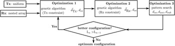
A three-step procedure is proposed as outlined in Fig. 3. The pattern is first optimized with respect to
 $\vec d_{Tx} $
and d
os
by means of a GA [Reference Haupt8] to fulfill the constraints in the transmitter array. Then, the same optimizer is applied to d
os
and
 $\vec d_{Rx} $
with the receiver constraints. Lastly, the optimum configuration can be found by applying the pattern search to d
uni
, d
sub
and d
os
. The search is conducted on a λ/4 grid. This configuration can be used as an initial array arrangement, and all three steps can be performed again to achieve a better solution. If an improved configuration with larger virtual aperture is found in the n
th attempt (L
n
>L
n−1), the optimization procedure performs the next attempt with an updated configuration. Otherwise the procedure is stopped and the last configuration is used. It was found that in most cases a solution to (1) is obtained after the first iteration, so that the loop is processed only twice.
Optimization procedure.

As a result, the optimization cost and time are dramatically decreased compared to a one-step optimization as the number of variables is reduced from (N + M) to (
 $\lfloor M/4 \rfloor + N/2 + 5$
). Because of the statistical property of the genetic optimizer, the whole procedure should be repeated several times to obtain the best configuration. The constraints can be slightly modified in the process as demonstrated in the examples below. One should note, however, that because of the complexity of the problem the solution most likely represents only a local minimum. In these cases, the redundancy of the array is not minimum, albeit is sufficiently low, in general.
B) Examples
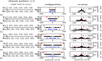
To validate the concept, the synthesis procedure is assessed in MATLAB. A MIMO Radar system with ten transmitters (N T = 5) and 13 receivers (M = 13) is examined. This yields k = 3 elements for the receiver sub-arrays 2 and 3 and a uniform spacing of d uni = 15λ/2 for the seven elements of the receiver sub-array 1. All antennas are considered as isotropic radiators.
As shown in Fig. 4(a), the nested structure is used as the initial system configuration with a large virtual aperture and a thinning rate exceeding 95%. However, redundancy is still observed in the virtual co-array, and the configuration can thus be optimized.
MIMO Radar system with ten transmitters (N T = 5) and 13 receivers (M = 13) and its co-array: (a) initial configuration, (b) only the transmitters are optimized, (c) only the receivers are optimized, (d) the whole non-uniform array is optimized without (system C0) and with element spacing constraint of (e) λ (system C1), and (f) 4 λ (system C2).

If the genetic optimizer is applied only to either the transmitter (optimization 1) or the receiver (optimization 2), the virtual aperture increases by more than 52% (Fig. 4(b)) and 125% (Fig. 4(c)), respectively. If the whole array is optimized, then the aperture can be increased by nearly 147% as illustrated in Fig. 4(d). The thinning rate then exceeds 98%.
In addition, system configurations with a minimum element spacing constraint of Δd = λ (system C1) and Δd = 4 λ (system C2) are shown in Fig. 4(e) and 4(f), respectively. The aperture of system C2 is 9% smaller than that of the configuration without constraint, whilst the aperture of system C1 is nearly 6% larger. The thinning rate varies between 97.9 and 98.2%. This observation indicates that for large N and M the search space is reduced when constraining the element spacing even to small values. This, in turn, improves the convergence of the GA. Thus, the design procedure can be performed for several Δd (Δd ≥ Δd min ) to yield the best array arrangement.
IV. JOINT FFT/MUSIC ESTIMATION
In this study, the range and the DOA are estimated by means of an FFT and a MUSIC algorithm, respectively. In comparison to 2D-MUSIC or 2D-ESPRIT, the proposed technique is suitable for real-time applications because of its lower computational effort. The procedure is summarized in Fig. 5.
The proposed signal-processing scheme.

A) Range estimator
The range of the objects is estimated by Fourier transform [Reference Stoica and Moses12]. The 1D-FFT spectrum can be defined as
 $$Z_q \left( r \right) = \sum\limits_{k = 0}^{K - 1} z_q \left( k \right) \cdot \exp \left( { - j2\pi rk/K} \right).$$
Here, Z q and z q denote the received signals of the q th virtual SISO element in the rth range bin and at the k th normalized frequency (k = 0, …, K − 1), respectively. Besides, q = nm (q = 1, …, NM) denotes the SISO element of the n th transmitter (n = 1, …, N) and the m th receiver (m = 1, …, M).
The range of the objects is allocated to range bins noted as r = r 1, …, r T for T detected peaks. The joint range/DOA estimation problem is transformed into T-independent DOA-estimation problems in range bin r t (t = 1, …, T).
B) DOA estimator
A combination of difference co-array and MUSIC is proposed to solve the DOA-detection problem [Reference Pham and Jacob4]. First, the co-array of the SISO array signals
 $\vec Z(r_t ) = \left[ {Z_1 (r_t ), \ldots, Z_{N \cdot M} (r_t )} \right]^T $
in range bin r
t
is constructed and renormalized to form a uniform virtual co-array of L elements with the amplitude distribution
 $\vec A_{co} = \left[ {x_1, \ldots, x_L} \right]^T $
.
Because of the non-linear processing path, the correlation between the sources deteriorates the image. To deal with this problem in the MUSIC spectrum, a forward–backward spatial smoothing technique as described in [Reference Pillai and Kwon11] is applied to the response of the virtual co-array. The effective aperture is however equal to the aperture P of the sub-arrays, which is limited by
 $\lfloor 3L/4 \rfloor$
as proved in [Reference Pillai and Kwon11]. The method can be summarized as follows:
-
• The virtual co-array of L elements is divided into (L − P + 1) overlapping sub-arrays of
 $P\;( \le \lfloor 3L/4 \rfloor$
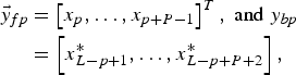
) elements as depicted in Fig. 6. The amplitude distributions
$\vec y_{fp} $
and
$\vec y_{bp} $
of the pth sub-array in forward/backward directions are
(3)with T being the transpose operator.
$$\eqalign{\vec y_{fp} & = \left[ {x_p, \ldots, x_{p + P - 1}} \right]^T, \;{\rm and}\; y_{bp} \cr & = \left[ {x_{L - p + 1}^\ast, \ldots, x_{L - p + P + 2}^{\ast}} \right]\comma}$$
-
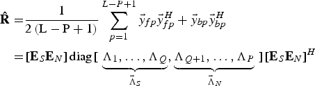
• The estimated correlation matrix
${\bf \hat R}$
is
(4)with H being the Hermitian operator and the subscripts S and N denoting the signal and the noise subspace, respectively. If the number Q of targets within the current range bin is known, the vectors
$$\eqalign{{\bf \hat R} = & \displaystyle{1 \over {2\left( {{\rm L} - {\rm P} + {\rm 1}} \right)}}\sum\limits_{p = 1}^{L - P + {\rm 1}} \vec y_{fp} \vec y_{fp}^H + \vec y_{bp} \vec y_{bp}^H \cr = & \left[ {{\bf E}_S {\bf E}_N} \right]{\rm diag}\left[ {} \right.\underbrace {\Lambda _1, \ldots, \Lambda _Q} _{{\bf \vec \Lambda} _S}, \underbrace {\Lambda _{Q + 1}, \ldots, \Lambda _P} _{{\bf \vec \Lambda} _N} \left. {} \right]\left[ {{\bf E}_S {\bf E}_N} \right]^H} $$
${\bf \vec \Lambda} _S $
and
${\bf \vec \Lambda} _N $
consist of Q and P–Q eigenvalues of the matrix
${\bf \hat R}$
with Λ1 > · · · >Λ
Q
>Λ
Q+1 > · · · >Λ
P
while
$\left[ {{\bf E}_S {\bf E}_N} \right]$
contains the corresponding eigenvectors.
-
• With
$\vec a = [1,\exp \left( { - j\pi \sin (\theta )} \right), \ldots, \exp \left( { - j(P - 1)\pi \sin (\theta )} \right)]^T $
being the DOA vector, the estimated angular positions
$\hat \theta $
of the far-field sources can be determined as peaks in the MUSIC spectrum:
(5)
$$\Psi \left( \theta \right) = \displaystyle{1 \over {\vec a^H (\theta ){\bf E}_N {\bf E}_N^H \vec a(\theta )}}.$$








Forward/backward spatial smoothing scheme.

The computational effort can be further reduced by applying other high-resolution spectrum estimation methods such as ESPRIT or Root-MUSIC instead of MUSIC after the spatial smoothing step. However, the estimation accuracy decreases slightly in scenarios having radar signals with lower signal-to-noise-ratio (SNR). More information can be found in [Reference Waweru, Konditi and Langat13].
V. EXPERIMENTS
A SAR setup is used for experimental validation at W-band (75–81 GHz) in our laboratory. The receive antennas are emulated by a W-band horn (gain of 21 dBi) mounted on a carriage rail [Reference Rezer and Jacob14]. A vector network analyzer (PNA E8361) serves as the transceiver with transmit power of 0 dBm and measurement bandwith of 1 kHz. Various equivalent SISO configurations can be easily composed with high flexibility. This configuration is equivalent to a MIMO system with TDMA scheme as mentioned above.
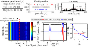
Because of the limited available space in the laboratory, the targets, composed of corner reflectors with an edge length of 3 cm (point targets) or metallic plates with a size of 13 × 11 × 5 cm3 (spatially distributed objects), are placed at a distance of only 3.3 and 4.1 m, respectively. Since far-field conditions are not met, the data have to be refocused [Reference Soumekh15]. Furthermore, for a given target scenario the array size is limited by the directivity of the horn antennas. Here, it was set to 0.3 m (85 λ at 79 GHz). Hence, an optimized array configuration with only six transmitters and 11 receivers is used as shown in Fig. 7(a). The thinning rate still reaches 96.9%.
(a) Experimental MIMO radar system with N = 6 transmitters (N T = 3) and M = 11 receivers and image of three corner reflectors (point targets), (b) received signals of SISO antennas over range, (c) MUSIC spectrum in the object plane, and (d) the eight largest eigenvalues of the covariance matrix.

Additionally, as a compromise between cross-correlation reduction and high resolution, a window length of P = (L + 1)/2 of the spatial smoothing scheme is chosen in the signal processing path. Finally, the image obtained by the dense SISO system with the same aperture is used as a reference.
The images of the three-point-target scenario over range and DOA are depicted in Fig. 7(b) and 7(c), respectively. Instead of only one peak at the angle of 4° detected by the dense SISO system without difference co-array processing and spatial smoothing techniques, two close targets are clearly resolved with the proposed system. This demonstrates a high angular resolution of better than 1°. The contrast between the peaks and the background in the image is however lower than the one of the filled SISO array with co-array processing.
The eigenvalues of the covariance matrix are related to the radar cross-section of the targets as well as of small scatterers in the background. As shown in Fig. 7(d), difference of more than 10 dB between the first (signal subspace) and the fourth eigenvalues (noise subspace) can be observed. This suggests that the number Q of targets, which is assumed to be known in this work, could be determined by applying a threshold Λ thr . This issue will be examined more closely in future work.
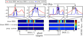
The images of two spatially distributed objects appear as groups of multiple scattered points (Fig. 8). Due to the lower SNR of the radar signal (longer distance) and higher cross-correlation noise in the non-linear processing path (more point scatterers), ghost targets are still observed in the image of the proposed system in contrast to the reference system. These observations underline the need of high SNR in the radar measurements with the sparse system.
Measurement results for two metal plates (distributed targets): MUSIC spectrum in the object plane of the proposed system (left) at position 1 and (right) at position 2 with a lateral offset Δd pos1,pos2 = 4λ( ≈ 6 cm).

Furthermore, as Fig. 8 demonstrates, the positions of the ghost targets change rapidly, whilst those of the real objects remain nearly unchanged if the radar system is displaced laterally by ≈ 4λ. This suggests that filter methods such as tracking over time or image correlation of sub-arrays allow to suppress the ghost targets.
VI. CONCLUSION
A novel MIMO radar concept combining a symmetric hybrid receiver array as well as two transmitter arrays in split configuration and employing difference co-array processing is presented. A periodically thinned and two non-uniform small sub-arrays are used to construct the receiver. Then a fast and low-cost three-step optimization procedure is implemented to determine an optimum array arrangement satisfying the system requirements such as high angular resolution and element spacing constraints. A large virtual aperture as well as a thinning rate in excess of more than 95% are achieved.
Finally, high-resolution images of three-point targets and of two spatially distributed objects are demonstrated in laboratory experiments. Additionally, the possibility of ghost-target suppression with e.g. tracking filter in scenarios of lower SNR radar measurement is also illustrated. In consequence, the validity of the proposed approach is confirmed.
 M. Nhat Pham received the Dipl.-Ing. degree in Electrical Engineering in 2011. Then, he joined in the Institut fuer Hochfrequenztechnik, Technische Universitaet Hamburg–Harburg, Hamburg, Germany, and is working toward the Dr.-Ing. degree. His current research interests include the signal processing and calibration methods for phased array systems.
 Arne F. Jacob received the Dipl.-Ing. degree in Electrical Engineering in 1979 and the Dr.-Ing. degree in 1986 from the Technische Universitaet Braunschweig, Germany. From 1986 to 1988 he was a Fellow at CERN, the European Organization for Nuclear Research, Geneva, Switzerland. In 1988, he joined Lawrence Berkeley Laboratory, University of California at Berkeley for almost 3 years as a Staff Scientist at the Accelerator and Fusion Research Division. In 1990, he became a professor at the Institut fuer Hochfrequenztechnik, Technische Universitaet Braunschweig. Since 2004 he has been a professor at the Technische Universitaet Hamburg–Harburg, Hamburg, Germany, where he heads the Institut fuer Hochfrequenztechnik. His current research interests include the design, packaging, and application of integrated (sub-) systems up to millimeter frequencies, and the characterization of complex materials.