

Introduction
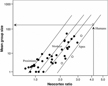
The Social Brain Hypothesis (Dunbar, Reference Dunbar1992, Reference Dunbar1998; Barton, Reference Barton1996; Dunbar and Shultz, Reference Dunbar and Shultz2007) provides an explanation for evolutionary pressures selecting for large brains within the order Primates, the order of mammals to which humans belong. It proposes that the principal selection pressure acting on the evolution of brains has been the cognitive demands of sociality. One outcome of this is a relationship between mean social group size for a species and its relative neocortex volume. The assumption underlying the Social Brain Hypothesis is that the computational capacity of a species’ brain (principally reflected in the volume of its neocortex) sets a limit on the number of individuals who can be held together in a coherent social group. The core evidence to support this is the fact that primates exhibit a distribution of group size in relation to relative brain size that is surprisingly consistent (Figure 1). The relationship between neocortex volume and social group size can be extrapolated to humans, and, based on the great ape regression equation, predicts a fundamental social group size of ~150 in modern humans (Dunbar, Reference Dunbar1993). There is a considerable body of evidence to suggest that this figure is characteristic of both natural human communities and personal social networks (Dunbar, Reference Dunbar1993, Reference Dunbar2008; Hill and Dunbar, Reference Hill and Dunbar2003; Roberts et al., Reference Roberts, Dunbar, Pollet and Kuppens2009).
Mean group size for individual primate genera plotted against neocortex ratio (ratio of neocortex to rest of brain). Open symbols: apes; closed symbols: prosimians (on left) and monkeys.
Source: see Dunbar (Reference Dunbar1992).

Presumably, species-typical group sizes, and the brains that underpin them, represent the outcome of an evolutionary tradeoff between the benefits of living in groups of a particular size (in the case of primates, principally a reduction in predation risk: Shultz et al., Reference Shultz, Noe, McGraw and Dunbar2004; Shultz and Dunbar, Reference Shultz and Dunbar2007) and the energetic costs of evolving and then maintaining the required additional brain tissue (Aiello and Wheeler, Reference Aiello and Wheeler1995). What is less clear is what is involved in the cognitive interface between brain size and social group size. The essence of the Social Brain Hypothesis is that what differentiates primate sociality from that of other species of animals (and hence requires that they have much larger brains for body size: Jerison, 1974) is that primate sociality is more complex. Exactly what that involves is, however, by no means obvious, though there is plenty of evidence to suggest that behavioural aspects of social complexity do correlate with relative brain size among primates (e.g. grooming clique size: Kudo and Dunbar, Reference Kudo and Dunbar2001; male mating strategies: Pawłowski et al., Reference Pawłowski, Lowen and Dunbar1998; the frequency of social play; Lewis, Reference Lewis2001; the frequency of tactical deception: Byrne and Corp, Reference Byrne and Corp2004; coalition formation: Dunbar and Shultz, Reference Dunbar and Shultz2007; social network structure: Lehmann and Dunbar, Reference Lehmann and Dunbar2009). Nonetheless, in principle, it has seemed reasonable to claim that, in some explicit sense, individuals’ abilities to compute and choose between alternative future social scenarios lie at the root of this. Some evidence to support this claim has now been provided by neuroimaging studies which have revealed correlations between the size of individuals’ socials networks and the volume of key brain regions known to be involved in social cognition (Powell et al., in press). Thus, there appear to be real cognitive constraints on social network size that are underpinned by what is colloquially referred to as the ‘wetware’.
Of more interest for present purposes, however, is the fact that social networks themselves are highly structured. Hill and Dunbar (Reference Hill and Dunbar2003), Zhou et al. (Reference Zhou, Sornette, Hill and Dunbar2005), and Hamilton et al. (Reference Hamilton, Milne, Walker, Burger and Brown2007) found that both human social networks and human grouping patterns consist of a series of hierarchically inclusive layers that have a scaling ratio of approximately 3. In effect, the ‘natural’ group size of ~150 that is characteristic of humans is, in fact, just one of a series of nested layers whose successively inclusive sizes are approximately 5, 15, 50, 150, 500, and 1,500 (Zhou et al., Reference Zhou, Sornette, Hill and Dunbar2005).
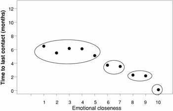
These layers are not equal in terms of strength of relationship. First, there appears to be a significant difference between relationships with those individuals who lie within the 150 layer compared to those who lie without. The 150-layer seems to delineate those people with whom an individual has a personalized relationship, a relationship based on some kind of shared history and personal knowledge with whom there is some element of obligation and reciprocity. Those who lie in the circles beyond 150 are known largely in terms of roles or categorical types: we recognize them as individuals and we may well be able to attach names to faces, but our relationship with them is categorical rather than personal (my hairdresser, my doctor, the person who serves in my local store, the one who reads the news on TV every night, someone I met once at a party, a work colleague) and may well be one-way (I know who they are, but they may not necessarily know who I am) and, importantly, the relationship lacks any intrinsic sense of obligation and reciprocity. Second, even within the 150, relationships are not homogenous across the layers (Figure 2). Hill and Dunbar (Reference Hill and Dunbar2003) and Roberts et al. (Reference Roberts, Dunbar, Pollet and Kuppens2009) have shown that these layers exhibit quite distinct patterns in terms of Ego'sFootnote 1 emotional closeness to, and frequencies of interaction with, individual network members. Both mean frequencies of interaction and typical values of emotional closeness fall off rapidly with network layer. Very roughly, the innermost layer of five intimates are contacted on a weekly basis, whereas the rate of interaction with the 15-layer (the next layer out) averages around once a month (Dunbar and Spoors, Reference Dunbar and Spoors1995), and contacts with those who lie in the 150 layer average only once a year (Hill and Dunbar, Reference Hill and Dunbar2003).
Mean time to last contact for individuals classified by Ego in different classes of a 1–10 emotional closeness scale for all individuals contacted at least once a year (N = 2,934 individuals). 1 represents low emotional closeness, 10 represents high emotional closeness. The circles enclose what stand out as different groupings. 50 individuals (1.7% of total sample) who were classified as emotional closeness = 0 have been excluded.
Source: Hill and Dunbar (Reference Hill and Dunbar2003).

The fact that ego-centric social networks of the kind illustrated in Figure 2 map onto natural human groupings (as implied by the analyses in Zhou et al., Reference Zhou, Sornette, Hill and Dunbar2005) might imply that organizations tend towards specific sizes. Indeed, on a more general note, it may well be that specific group sizes are more efficient for certain activities than for others, depending on the level of personal and emotional engagement required by the task, leading to a natural tendency for groups of a particular type to cluster around particular sizes. In addition, the fact that networks are as highly structured as they are, and that this structuring is explicitly tied to frequencies of interaction, suggests that there may be limits to the rate with which novel social institutions will flow through the system. This is directly relevant to Grannoveter's (1973) suggestions about the role of weak ties in information exchange in networks. I return to this point in a later section. First, I discuss in more detail the size and structure of natural human groupings.
Natural groupings
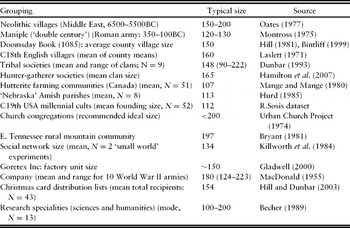
Table 1 summarizes a range of data that identify a consistent grouping size in human social organization of between 100 and 200 (the 95% confidence limits around the predicted value of 150 based on the ape social brain relationship) across a wide range of social and historical contexts. These may be labelled in different ways, but their essential structure is much the same – a community that shares a common purpose or function.
Examples of human social groupings that conform to the predicted size of ~150 individuals1

Notes: 1Confidence intervals around the predicted mean are 100–200 (Dunbar, Reference Dunbar1993).
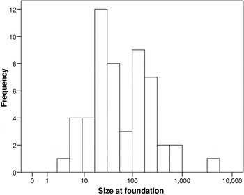
Figure 3 illustrates this with a more homogenous dataset on the founding sizes of American nineteenth-century utopian cults (see Muncy, Reference Muncy1973). These include both explicitly secular as well as religious sects. They have a mean value of 112 (range 4–5,000, N = 53). However, the data are strongly skewed (one sample Kolmogorov–Smirnov test against a normal distribution, p = 0.005): the median value is 41.5 (i.e. rather closer to the 50-layer), with small values (sizes <15) being especially uncommon. In fact, Figure 3 clearly suggests that the distribution is actually bimodal (with modes at ~50 and ~150). These results suggest two conclusions. First, there is a minimum size that cults can have at foundation (typically not less than 15 members), and, second, that there may be optimum sizes that work best which cluster around the 50 and 150 layers identified by Zhou et al. (Reference Zhou, Sornette, Hill and Dunbar2005). There is some suggestion in these data that this difference may relate to secular and religious cults, respectively.
Distribution of cult community size at time of foundation, for 53 nineteenth-century American utopian cults.
Source: Sosis and Alcorta (Reference Sosis and Alcorta2003).

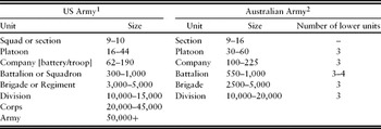
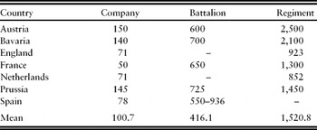
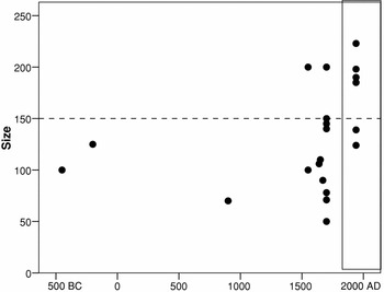
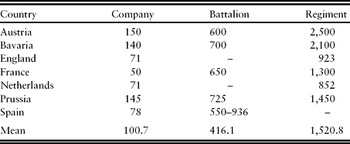
Military organization provides a particularly clear example of the suggestion that there are natural grouping sizes that work best, since performance on the battlefield must be among the most demanding of circumstances: not only does success depend on getting coordination within and between fighting units right, but men's lives are at stake. The structure of military units in historical as well as contemporary armies seems to mirror quite closely both the numerical values and the scaling ratio identified by Zhou et al. (Reference Zhou, Sornette, Hill and Dunbar2005) for natural human groups (Tables 2 and 3). Of particular importance in this context is the size of the company, the smallest military unit that can act independently. Figure 4 plots the range of company sizes for a sample of World War II armies (boxed set on right side). These have a mean of 177.7, and the variance around this is modest (SD = 34.4), although there is perhaps the hint of two separate groupings (the lower set compromising Britain and Russia; the upper set comprising USA, Japan, France, and Germany). Both Germany and the USA reduced the sizes of their companies (from 223 to 193, and from 185 to 147, respectively) well before the end of the war, apparently to improve coordination within units rather than simply because they were running out of conscripts (an especially unlikely scenario in the case of the USA). Figure 4 also plots the typical size of companies through time, including early examples of basic fighting units from armies of the classical period. It seems as though military planners have experimented with various sizes, and gradually settled on one – presumably the one that works best on the battlefield. Note that in the early modern period (i.e. around 1700) before the introduction of electronic communication systems to facilitate coordination among the members of a fighting unit, company sizes were significantly smaller (mean 122.8 ± 57.1 SD) than they were in mid-twentieth century (t = –2.38, p = 0.033 with unequal variances).
Organizational structure of modern armies

Notes: 1Department of the Army (1994); 2http://www.awm.gov.au/atwar/structure/army_structure.asp#basic.
Structure of European armies during the War of the Spanish Succession (c.1702)
Mean company size in World War II armies (right-hand column), and in European armies during some earlier periods. On the left are the basic fighting units of the classical period armies of Persia (sabatam: c.450 BC) and Rome (maniple: 350–100 BC), and of the Vikings (hafna: c.900 AD). Boxed on the right are armies of the main protagonists at the outset of World War II.
Source: MacDonald (Reference MacDonald1955), supplemented by additional online information.

Military organization also provides a clear example of the fact that higher order groupings can be constructed (battalions, regiments, divisions, etc., at numbers approximating 500, 1,500, and 5,000: Table 2). However, this is only possible through the imposition of very strictly hierarchical line management (the creation of a hierarchy of officer categories that mirrors the grouping levels) combined with strict discipline (orders from higher up the command system must be obeyed without question, on penalty of very severe punishment). This point is well made in the context of the Hutterites, who deliberately split their communities once they exceed 150 in size because, so they allege, it is impossible to control a larger community by peer pressure alone, but instead requires a police force and imposed discipline of a kind that is anathema to their communalistic ethos (Mange and Mange, Reference Mange and Mange1980).
In sum, these data thus suggest (1) that there is a consistent natural size to human groups, (2) that these groups are themselves structured in a distinct pattern of hierarchically inclusive layers, (3) that there may be optimal group sizes that depend on the functions being subserved that may well reflect the levels of trust and reciprocity required for that particular function, and (4) that higher-order groupings (i.e. above 150) are possible, but require the external imposition of discipline and punishment to maintain coherence and cooperation through time.
Information flow
In his classic paper, Grannoveter (Reference Grannoveter1973) distinguished between two kinds of relationships that individuals might have with each other (strong ties with intimates and close friends, and weak ties with acquaintances) and argued, on the basis of survey data on where jobless individuals gained their information about available jobs, that weak ties played a uniquely important role in information flow through communities and networks. Such information did not generally come through strong ties. Information about the availability of job opportunities is, in some sense, a specialized aspect of modern social life. However, it might be seen as standing for a more general sense of information flow at a wider level, including rumour, knowledge about new products or social events, new ways to behave, etc., that have a rather older and more general relevance to us as individuals. We can therefore ask whether there is a limit on how far out Ego can acquire information when networks are structured in the way they appear to be.
To explore the implications of network structure for the rate at which information might flow through a community, I modelled the likelihood that Ego (at the centre of the network) would find out about some novel item of information through direct face-to-face contact for communities of different sizes (5, 15, 50, 150, 500, 1,500, and 5,000 individuals), given layer-specific rates of contact. The probability of discovering some novel fact from individuals up to an including layer i in the network, Plearn [i], is taken to be the cumulative conjoint probability of encountering any given individual in a network layer of size n and the likelihood that any one of these individuals would know the fact in question
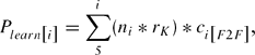
where ni is the number of individuals in the ith network annulus or layer, rK is the likelihood that any one of them will know the fact in question (here taken to be constant, and equivalent to rK = 0.01), ci [F 2F ] is the likelihood of contacting any given individual face-to-face, with this function summed across successive layers of the network from the innermost layer (the layer of 5 most intimate Alters) up to and including layer i. Note this model views information as a static property of an individual: information is not actively passed on from one Alter to another within the network. Although obviously a radically simplified assumption, for present purposes it provides a ‘first pass’ assessment of the likelihood of discovering some vital fact about the world.
I parameterized the model using data on the frequencies of face-to-face interactions obtained from a large sample (N = 251) of female ego-centric networks from Belgium and the UK. Only women aged 18–60 years were sampled. In addition to listing all members of their network, Egos were asked to specify when they last saw each individual Alter and how emotionally close they felt to them on a 1–10 scale (for details, see Roberts et al., Reference Roberts, Dunbar, Pollet and Kuppens2009). Time since last contact was transformed to yield a rate of contact per annum. I used the emotional closeness categories to define the layers of each Ego's network by dividing the Alters ranked in order of declared emotional closeness into the first 5, the next 10, 35, and 100 to yield the successive annuli in the personal network, and then calculated the mean rate of face-to-face contact with members of each layer, averaging across all Egos.
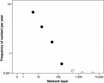
Figure 5 plots the mean rate of face-to-face contacts with members of the four core network layers of the network (the 5, 15, 50, and 150 layers), and extrapolates this observed pattern out through the next three layers (500, 1,500, and 5,000). The rate of contact declines exponentially, with the drop in contact frequency being nearly 50% between the 5 and 15 layers alone. Contacts with members of the outer layers (especially those beyond the 150) are extremely low – in the order of years rather than months between contacts. Thus the rate at which information flows through the system is likely to depend on how deeply structured it is (i.e. how steep the fall off in encounter rates is) and on the size and connectedness of the layers.
Probability of face-to-face contact with a randomly chosen member of the successive circles of acquaintanceship, for the sample shown in Figure 2. Solid symbols indicate observed data; open symbols: data extrapolated to larger layers from the regression equation fitted to the observed data.

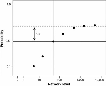
I then used these values in equation (1) to calculate the cumulative probability distribution across network layers (i.e. assuming that, successively, Ego only has access to the first 5, 15, 50, 150, 500 . . . etc. members of his/her extended social network). Figure 6 plots the results. The probability of acquiring information reaches an asymptotic value at a community size of ~1,500, with little further gain in the likelihood of hearing about an innovation as community size increases beyond this. The inflexion point (the point at which the marginal gain begins to diminish) can be identified as the value of the X-axis where the asymptotic value on the Y-axis is reduced by 1/e: here, this occurs at a community size of exactly 50. In other words, the gains to be had by increasing community size beyond ~50 diminish exponentially and become trivial beyond a community size of ~150 individuals. These results thus suggest that, if face-to-face information flow is the issue, then communities larger than about 150 are likely to be of limited value in any context where communication depends on face-to-face interaction. Since this pertains universally in traditional small-scale societies, this suggests that there has probably been little or no selection pressure favouring further increases in the capacity to broaden or deepen communication. Rather, the principal selection pressure has been for community sizes at least up to 50 individuals, and perhaps up to 150.
Cumulative probability of acquiring an item of knowledge through face-to-face interaction with an individual who has that knowledge in communities of different size (5, 15, 50, 150, 500, 1,500 and 5,000), based on the contact rates shown in Figure 5. The model assumes that 1% of all community members are knowledgeable.

This analytical model, however, offers only a static analysis. It assumes that information does not flow through the system while Ego is searching for it; instead, it assumes (rather unrealistically, perhaps) that community members do not talk to each other and so cannot learn useful facts from each other. To explore what happens when knowledge can flow through the network while Ego is searching for it, we used a Monte Carlo simulation. However, the inevitable complexity of a model in which information can flow in all directions means that we need to make compromises in other respects. In this case, we have chosen to limit the range of possible sources of information available to an individual (in effect to the two innermost layers of the social network, the 5 and 15 layers) and so have ignored the less frequent contacts that might occur between weak links.
Most classic models of cultural evolution (e.g. Cavalli-Sforza and Feldman, Reference Cavalli-Sforza and Feldman1981; Boyd and Richerson, Reference Boyd and Richerson1985) have used mean field models whose dynamics derive either from epidemiology or from conventional population genetics. Such models assume random ‘mating’ throughout the network (everyone has an equal chance of meeting and exchanging information [or genes] with every other individual in the population). However, in most real world situations, random mating is constrained by the spatial or social structure of the population. Our model imposes structure by limiting the number of individuals that Ego can sample when choosing what behaviour to adopt. We did this by the simple device of setting individuals at the nodes on a lattice (formally, a torus in which all the edges join up with their opposite edges) and then limiting their interactions to the individuals at adjacent nodes, with declining probabilities of interaction with nodes at successive steps removed (i.e. differentiating immediate neighbours from neighbours of neighbours). In each generation, individuals acquire (learn or copy) a trait either by adopting that of the individuals around them (copying) or by personal discovery (i.e. ‘mutation’). Note that although the model is conceived as a spatial model (nodes are on a physical lattice), in fact this can equally well be interpreted as a social lattice in which interactions are restricted to certain classes of individuals (who are represented as adjacent nodes on the lattice, just as we might do so in a social network diagram). We used a lattice of size 100 × 100, and thus a total population size of N = 10,000 individuals.
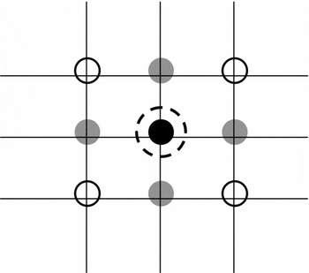
The population was initialized with all nodes seeded with cultural variant d, with a mutant variant c seeded in the population with a probability of p = 0.0001. At each successive generation (i.e. iteration), each node reproduces and is replaced by a cultural ‘offspring’. The cultural variant of this offspring is determined by the probability of acquiring variant c at that site. It can acquire variant c either by mutation (with a very low probability determined by a pseudorandom number in the interval [0, 1]) or by cultural inheritance (biased transmission) from adjacent nodes. This second transmission probability is determined by the cultural variant of the previous occupant of that node (the ‘cultural parent’) and those of its eight immediate neighbours on the lattice (Figure 7). In the latter case, we distinguish two kinds of neighbours: those whom Ego can contact directly (the four nodes directly connected to Ego on a vertical or horizontal lattice edge) and those whom Ego can only access through its immediate neighbours on the lattice (i.e. friends of friends, identified here as the four nodes on the diagonal corners of the square centred immediately around Ego). In effect, these two types of neighbour correspond to friends and friends-of-friends, respectively. The probability of acquisition (copying) depends on the source's network position, and these are defined as a 0, a 1, and a 2 for the three types of neighbours (parent, friend, and friend-of-friend) respectively, subject to the constraint that the weights for all nodes sampled sum to ∑ak = 1. In order to assess the impact of different gradients in the transmission frequencies across the three model types, we used three different weight profiles, wi, defined by the sets w 1 = [a 0 = 0.76, a 1 = 0.04, a 2 = 0.02], w 2 = [a 0 = 0.52, a 1 = 0.08, a 2 = 0.04], and w 3 = [a 0 = 0.20, a 1 = 0.10, a 2 = 0.10], chosen to reflect a range of gradients from steep to shallow. For each weight distribution, 100 simulations, run to fixation (pc = 1), were performed. The details of the model are given in the Appendix.
The different sources of influence used in the agent-based model of cultural evolution. Nodes on a lattice surrounding Ego (identified by the large broken circle on the centre node) provide sources of influence in biased transmission of trait type according to three types of relationship: cultural parent (previous occupant of the node: black), immediate neighbours with whom Ego can interact directly (grey nodes connected to Ego via lattice edges), and neighbours of neighbours (unfilled circles, with whom Ego can interact only indirectly through a neighbour node).

We can show that this model produces identical effects to those of Boyd and Richerson's (1985) mean field model under the same conditions of panmictic ‘mating’. That is to say, when we relax the spatial constraint and allow everyone to interact with everyone else with equal probability (i.e. probabilities of acquisition a 0 = a 1 = a 2 . . . = aN), our computational agent-based model gives the same pattern and time to fixation by a mutant cultural variant as you would get with Boyd–Richerson's strictly analytical model of direct biased transmission parameterized with the same values. This is important, since it allows us to be sure that if our spatially structured computational model produces different results from a classic Boyd–Richerson analysis, this must be due to the spatial structure and not simply due to some trivial peculiarity in the way the computational model has been constructed.
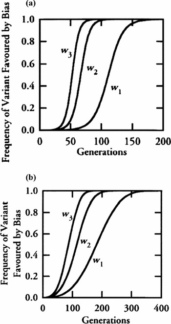
The mean (generational) rate of change in the frequency of variant c, p(i), for a standard panmictic model is shown in Figure 8(a). As would be expected under positive selection, the frequency of the mutant variant c increases to full penetrance over time (typically 75–150 generations, depending on the transmission probabilities involved). In contrast, for the same parameter values, penetrance is significantly slower in a spatially structured population than in a panmictic population, as indicated by the X-axis scale in Figure 7(b). Note that the mean values in Figure 8(b) do not include the large fraction of simulations that resulted in the extinction of variant c: extinction rates were 44% for set w 1, 53% for set w 2, and 60% for set w 3. Extinction is a key feature of all stochastic models, whether or not the models include population structuring, and is itself an important feature of stochastic environments. These extinctions arise mainly because the mutant trait disappears before it has managed to build up sufficient numbers of descendents to influence copying rates in the following generation(s).
Time taken to fixation for a mutant cultural variant under (a) a Boyd–Richerson (mean field) model of vertical transmission with direct bias and (b) in a spatially structured population based on Monte Carlo simulation with n = 9 cultural models for each individual on a 100 × 100 lattice matrix, for three different transmission weights (w 1: a 0 = 0.76, a 1 = 0.04, a 2 = 0.02; w 2: a 0 = 0.52, a 1 = 0.08, a 2 = 0.04; w 3: a 0 = 0.20, a 1 = 0.10, a 2 = 0.10). See Appendix for details.

We chose both the size of the population (N = 10,000) and the number of cultural influences (n = 9) for computational convenience. Changing lattice size and the number of cultural parents has a quantitative, but not a qualitative, effect on the transmission dynamics (for details, see Appendix). Having a smaller number of cultural parents, for example, slows the rate at which the population converges to full penetration by the novel cultural variant, but does not change the fact that the model will eventually converge. Conversely, choosing a larger number speeds up the rate of penetration, with a limit converging on the Boyd–Richerson solution when n equals all nodes in the lattice (i.e. panmixia). (For further discussion of other structural parameters on the model's performance, see the Appendix.)
These results suggest that population structuring is likely to play a critical role in determining the rates at which cultural information flows through a system. In fact, it seems intuitively likely that mean field models of the Boyd–Richerson type are simply the limiting case for structured population models: mean field models are equivalent to structured population models in which each individual is directly ‘linked’ to every other individual in the population. It should be no surprise, therefore, that the rates of cultural transmission are consistently greater in mean field models than in structured population models.
The important implication here is that information transmission is greatly slowed down in structured populations, even if we ignore all those cases where the innovation peters out and goes extinct. Indeed, the relatively high rates of novel variant extinction in the models (typically in the region of 50%) are a further reminder that, in stochastic universes, novel cultural items can often fail to spread even when there is significant selective bias in their favour. Since real world situations are typically stochastic rather than deterministic, this should remind us that cultural evolutionary processes are not necessarily always as fast as we sometimes suppose.
Conclusions
In this paper, I have tried to make two points. First, the social world that we experience as individuals is a great deal smaller than it might seem to be when we view it top–down in terms of large-scale political structures. Ever since the ‘six degrees of separation’ phenomenon became widely known (the fact that we can reach anyone in the world through six successive contacts: Travers and Milgram, Reference Travers and Milgram1969; Watts, Reference Watts2004), we have become used to thinking in terms of networks of contacts that rapidly extend like a spider's web across the entire world, eventually connecting up all six billion of us into a single integrated network. While in one important sense this is of course true, it is not necessarily the case that my knowledge of other individuals really extends anything like so far, never mind my willingness to behave altruistically towards them. The second is that just because someone somewhere in that enormous network has discovered some new fact or cultural trait does not mean that I will inevitably learn about it. In the absence of electronic communication, real everyday social life is very small scale. The six degrees do not necessarily mean that information flows at a uniform rate through the network. The structuring and clumpiness that characterizes real social networks has the inevitable effect of slowing down the rate at which cultural innovations or information flow through the community. I showed this with both a static model (parameterized with actual face-to-face contact frequencies) and a dynamic agent-based model (with a narrower range of transmission processes), and both yielded broadly similar results. (I will leave aside for present purposes the question as to whether electronic communication and social networking media allow us to cut through that constraint.)
These two points may be particularly important in the context of gene-culture coevolutionary models. These have tended to assume that the domain in which cultural social learning occurs is relatively large (‘the tribe’), although the exact numerical size of this population unit is never actually stated (e.g., McElreath et al., Reference McElreath, Boyd and Richerson2003). In the ethnographic literature, the tribe is defined as all those people who speak the same language (or dialect in the case of large language groups), and this turns out to correspond to the 1,500 layer in our analyses (see Dunbar, Reference Dunbar1993). Thus the tribe is in practice probably very much smaller than most of these analyses assume. More importantly, it is clear from our network data that interaction frequencies are very heterogeneous within even this small population. Indeed, most interactions (the source of most cultural learning) are actually confined to an even smaller subset of the population (principally the innermost 50 individuals, but certainly not much beyond the 150). Thus the true range of models available for copying in cultural transmission processes is actually confined to a group of individuals who represent only about 10% of the entire tribe, even given this more restricted definition of what actually constitutes a tribe. If doubt remains over this, it should be dispelled by the empirical evidence showing that the spread of both obesity and happiness through networks is limited to the first three degrees in the social chain (Christakis and Fowler, Reference Christakis and Fowler2007; Fowler and Christakis, Reference Fowler and Christakis2010a), although in practice the magnitude of the effect from the third degree is marginal even if significantly above zero. Second degree relationships appear to be equated with the 50 layer (essentially, friends of friends), and third degree with the 150 layer (friends of friends of friends).
This is not to say that social learning (and indeed cooperation) may not extend beyond these limits to a wider population. Rather, the point is that the levels of both copying and, especially, cooperation that occur at this wider level may be very much less frequent than we often usually suppose and may be subject to more stringent evaluation of the tradeoff between the costs and benefits. Altruism and concern for others principally extends to relatives (for reviews, see Strassman and Stearns, 1998; Barrett et al., Reference Barrett, Dunbar and Lycett2000), and relatives, even in contemporary western societies, are invariably encompassed within the 150 layer (as indeed they are in all traditional small-scale societies). Indeed, Fowler and Christakis (Reference Fowler and Christakis2010b) found that willingness to reciprocate in a public goods game extended only to second degree relationships (friends of friends). Similarly, in a review of altruistic behaviour in a wide range of historical and contemporary societies, Barrett et al. (Reference Barrett, Dunbar and Lycett2000) noted that unqualified altruism invariably occurred only between biological relatives, whereas altruism towards unrelated familiars was invariably explicitly reciprocal.
Unfortunately, in discussing the opportunities that individuals have of meeting and cooperating with others in small-scale (especially hunter-gatherer) societies, commentators have often misunderstood the nature of these social systems: they usually assume that the camp group or band (typically 25–50 in size) is the basic social unit, and so argue that the fact that individuals and family units frequently travel long distances (up to 200 km) to join other camps means that they have considerable opportunity to meet strangers towards whom they behave altruistically. In fact, it is the clan or community of 150 that constitutes the basic level of social grouping, the band or overnight camp group simply being a temporary subset of this population unit (Aurelli et al., Reference Aureli, Schaffner, Boesch, Bearder, Call, Chapman, Connor, Di Fiore, Dunbar, Henzi, Holekamp, Korstjens, Layton, Lee, Lehmann, Manson, Ramos-Fernández, Strier and van Schaik2008; Layton and O'Hara, Reference Layton, O'Hara, Dunbar, Gamble and Gowlett2010). Similarly, in discussing the !Kung San hxaro system of exchange (long-term dyadic exchange partnerships), Fehr and Henrich (Reference Fehr, Henrich and Hammerstein2003) note that the area over which the average couple's 48 hxaro relationships extend commonly covers an area of around 10,000–15,000 km2, and so encompasses a population of something in the order of 1,500 individuals. They argue on this basis that individuals must inevitably have many contacts with ‘strangers’, with whom they may cooperate or exchange altruistic acts (e.g. being allowed to use the local resources of the host camp). However, this misunderstands the structure of hunter-gatherer societies, since 1,500 is precisely the limit on the number of people that an individual might know by sight from personal contacts over the longer term. These are not strangers, but the wider community (or ‘tribe’) with whom an individual has definable relationships. Moreover, since this is also the pool from which individuals normally choose their ‘marriage’ partners,Footnote 2 everyone in this extended community is linked together through ties of affinal kinship, with all the obligations that these entail: offending a friend of a friend is to risk undermining one's relationship with the friend. Cooperation and altruism does not occur among casual strangers in the way these authors seem to imagine.
A second issue that may have clouded discussion in this context concerns exactly what is being exchanged in altruistic or cooperative interactions. A central premise of evolutionary biology (‘Hamilton's Rule’) reminds us that the level of any such investment will be titrated against both the costs and benefits that derive from the investment, as well as the opportunity costs incurred. The bottom line is that cheap acts of altruism will be exchanged proportionately more widely than expensive ones. This distinction is not always made as clearly as it should be in the literature, and has been somewhat confused by economists’ assumption that the opportunity cost incurred by wasting a small fee provided by the experimenter is a genuine cost in biological terms. In fact, the worst a subject in such an experiment can ever do is to be cost-neutral (even if they do waste an hour of their time). It is noteworthy that it has repeatedly been found that, in public good experiments, cooperation can only be maintained at even modest levels if punishment or social castigation are available as tools to enforce it (Orstrom et al., 1994; Fehr and Gächter, Reference Fehr and Gächter2000, Reference Fehr and Gächter2002). The level of altruism in such contexts is thus at best marginal in biologists’ terms.
We can, of course, create larger communities within which exchanges and cooperation occur, even beyond the 1,500-individual level. But such arrangements are invariably built around shared norms in some form (as markers of community membership, and hence trustworthiness and obligation) (Orstrom et al., Reference Orstrom, Gardner, Walker and Arbor1994; Orstrom, Reference Orstrom2003; McElreath et al., Reference McElreath, Boyd and Richerson2003), and they invariably have to be enforced by imposed discipline and punishment. Military organization provides an explicit example of this, as does the fact that Hutterites split their communities once they get above 150 precisely because they would require a police force to maintain prosocial behaviour if they did not.
The findings I present here have at least two general implications for the structure and evolution of social institutions. First, there may be optimal sizes and structures for institutions. If the organization is below about 150 individuals, then informal management structures may work very effectively. Of particular importance in this respect is the sense of community, of ‘belongingness’, that such institutions will have: as a result, individuals will feel a greater sense of obligation towards each other and may cooperate more effectively in achieving the institution's goals. Shared cultural markers of various kinds may be important both in identifying other community members and in engendering a psychological predisposition to cooperate (Nettle and Dunbar, Reference Nettle and Dunbar1997; McElreath et al., Reference McElreath, Boyd and Richerson2003). However, once an institution's size exceeds ~150, then formal management structures are needed to solve two key problems associated, respectively, with different kinds of information bottleneck (I will refer to these as casual and deliberate bottlenecks). One is the fact that, in large organizations, information simply does not flow where it should, even if everyone is keen for it to do so. This is especially important in the case of the kinds of casual conversations that are often responsible for imparting crucial but quite unexpected items of information. Such casual information bottlenecks may be quite unintended, but they arise simply because of lack of opportunity for face-to-face interaction. This is the problem of having too small a watercooler: not enough people can gather around it. The second problem is that rivalries are more likely to build up because individuals owe loyalty to their immediate group (the 150) and this automatically creates what amounts to in-group/out-group effects whenever sections of an institution come into conflict. Indeed, irrespective of any conflict or rivalry that might exist, they might arise simply because, in very large organizations, a natural in-group/out-group division emerges between those who encounter each other often (the 150) and those who are, effectively, strangers (the rest). Unintended in-group/out-group effects of this kind will unavoidably give rise to reduced cooperation and the development of deliberate (as opposed to casual) information bottlenecks.
Second, if information flow is important for an institution, then the precise choice of numerical size and the way this community is structured may be critical for how efficiently information flows through it (see also Lu et al., Reference Lu, Roberts, Cheng, Dunbar, Lió and Crowcroft2009). While the rates of interaction may differ in political or business organizations compared to the everyday social world, the fact is that all these institutions involve relationships between individuals, and relationships of all kinds are costly to maintain in terms of time investment. All that will change is the scale of the outcome. As a result, there may be optimal group sizes for particular types of communication: an organization that deviates in size from one of the ‘natural’ layers may result in less efficient information flow. If organization size is significantly below one of these numbers, there will be a reduced likelihood that some key fact which might later prove crucially relevant to the community will be discovered. On the other hand, if the organization is too large, information flow within the community will be slowed down: the core individual may never find the person who has that knowledge within the requisite time frame. These two sources of constraint are somewhat analogous to the well-known search time and handling time constraints in foraging contexts that are responsible for defining optimal foraging strategies (Stephens and Krebs, Reference Stephens and Krebs1986).
Finally, it is worth reminding ourselves that, in institutional life as well as in everyday life, interactions are invariably stochastic, and this inevitably has particularly important implications for the rate at which information can flow through an organization. This must be especially important for the spread of innovations, since these are both unpredictable in where they occur and subject to the vagaries of interaction between knowledgeable and naïve individuals. This must mean that innovations spread and achieve penetrance (100% adoption) at very much slower rates than most conventional mean field models imply. In particular, stochastic models are subject to serendipitous extinctions that do not feature in more conventional algebraic models. Our models suggest that novel traits (mutants) may have to be seeded (mutate) many times before they finally take off. In some runs of our agent-based models, the novel trait went extinct as many as 13 times before it finally built up enough demographic weight in the population to take off, despite the fact that the mutant trait was always advantageous.
Appendix: Monte Carlo simulation modelFootnote 3
Following the notation of Boyd and Richerson, the variants of a dichotomous trait are denoted by c and d, which occur in the population with frequencies p and q, respectively. For present purposes, c denotes the variant favoured by bias. The parameter B (where 0 ≤ B ≤ 1) is a measure of the effect of biased transmission. Each individual in the population acquires its cultural variant from n cultural parents. The probability that an individual is characterized by variant c, given exposure to the set of cultural parents {X} with cultural variants X 1, . . . , Xn, is
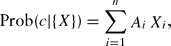
where Xi = 0 if the ith model is variant c and Xi = 1 if the ith model is variant d, and the importance factors, Ai, are given by
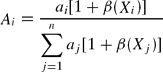
with
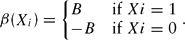
The parameters ai are the weights associated with vertical transmission from each of the cultural parents Xi. The frequency of variant c in the population after biased vertical transmission, p’, can be written as

For specific values of n, B, the basic weights ai, and the value of p in the ith generation, equation (1) can be used to determine the value of p in the (i + 1)th generation. For the trivial case where n = 2, the frequency of variant c after a single vertical transmission event is given by

This process assumes non-overlapping generations. If, instead, we treat both the variant frequency, p, and time as continuous variables and allow for overlapping generations, we can solve the analogous overlapping generations vertical transmission model explicitly for p in terms of the generational time, t, and the initial variant frequency p 0 at time t = 0

where
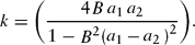
The Monte Carlo algorithm proceeds as follows. For the initial conditions, each individual (or node) in the L = N 2 lattice is given the variant value d, except for a single randomly chosen node which is assigned the mutant variant c. At each iteration (or generation), a new occupant is placed at each site. The cultural variant of the new occupant at a given site is determined by the local probability of acquiring variant c at that site and the selection of a uniformly distributed pseudorandom number on the interval [0, 1]. The transmission probability at a given site is determined by the cultural variant of the previous occupant, its nearest neighbours, and next-nearest neighbours, with corresponding weights a 0, a 1, and a 2. The weights are subject to the same constraint as in the standard mean field model, namely

with the sum extending over each of the n cultural parents. If we define σx,y(i) to be the cultural variant (c = 1, d = 0) at site (x,y) at generation i, we can express the local transmission probability for acquiring variant c in generation [i + 1 ], Px,y(i + 1), as

where the first sum with index j runs over all nearest neighbours of site (x,y), and the second sum with index k runs over all next-nearest neighbours of (x,y). The weight factors Al(i) are given by the expression
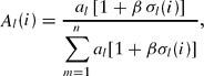
where the sum in the denominator runs over all n cultural parents, and the al represent the transmission weights. For present purposes, we used
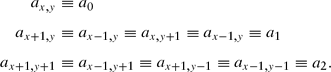
In this way, the algorithm generates new occupants (i.e. offspring) for every site in each generation, subject to the cultural transmission rules.
In a Monte Carlo model, the choice of pseudorandom number generator can be critical. Our choice was the multiplicative congruential generator of Kalos

with modulus m = 248 and multiplier a = 1113. This generator has been used extensively in Monte Carlo studies at the Courant Institute and, in particular, has passed all the standard tests for randomness (Knuth, Reference Knuth1969).
The only non-obvious aspect of our Monte Carlo algorithm is the data structure employed to store the lattice configuration at each generation. In order to store complete lattice configurations for each generation of the population, we maintain a ‘bit map’ of the state of the lattice, as this allows for efficient data storage. That is, each cell in the lattice is assigned one bit, which is set to 0 if the occupant of a cell is characterized by variant d and is set to 1 if the occupant of the cell is characterized by variant c. Blocks of bits are then stored compactly as words. Relatively fast operations (shifts and logical operators) can then be used for data manipulation and calculations of the occupants of lattice sites in future generations. The use of bit operations and storage methods has both improved computation speed and allowed for an easy transition to the study of large populations.
In addition, this compact method of data storage allows us to look in detail at the dynamics of cultural evolution (such as variant clustering behaviour) from a spatial or structured population perspective. Of course, it is recognized that this data storage scheme is appropriate only for studies of dichotomous characters; however, it should be noted that only minor modifications of this data structure have been required for our initial studies of simple two-state ‘dilute’ models.
Lattice structure, periodic boundary conditions and other considerations
The analysis of spatially structured systems in other areas of science reveals that both the equilibrium behaviour and the dynamics of the system depend on the dimension and connectivity of the system. In the case of regular lattice models, the important considerations are generally the lattice dimension, D, the lattice coordination number, q, the lattice size, N, and the lattice boundary conditions. While it is clear that it is beyond the scope of a preliminary study of the dynamics of a spatially structured system to report in detail on the effects of varying the lattice parameters, it is appropriate to discuss briefly the consequences of changing the lattice structure.
If all other lattice structural parameters are held constant, changes in lattice dimension will have no effect on the system dynamics. If we choose a particular lattice type (for example, regular lattice structures with q = 2D), then increasing the lattice dimension reduces the value of t 1/ 2 (the time taken to achieve 50% penetrance by variant c). In the limit as D → N, the value of t 1/ 2 approaches the mean field (Boyd–Richerson) result, assuming that the n cultural parents are chosen at random.
If N is held constant, increasing the coordination number (q) of the lattice effectively reduces the average number of ‘links’ between any two individuals in the population. Therefore, increasing q decreases the value of t 1/ 2. In the limit as q → N, the value of t 1/ 2 again approaches the mean field (Boyd–Richerson) result, assuming that the n cultural parents are chosen at random.
The Boyd–Richerson mean field model of cultural transmission is continuous, and therefore strictly applicable only to infinite populations. In contrast, a stochastic, spatially structured model is discrete, and the dynamics of the system are inevitably sensitive to system size. If other lattice and transmission parameters are held constant, the value of t 1/ 2 increases with increasing population size N. In fact, finite size system scaling considerations lead us to expect the value of t 1/ 2 to scale as a function of system size (to first-order approximation) as

where A and b are positive constants. Preliminary analysis of the dynamics of our spatially structured cultural transmission model for different population sizes confirms the predictions of this scaling law.
If some type of periodic boundary conditions are imposed (e.g., regular, spiral, skew), each unit in the population has the same number of nearest neighbors, next nearest neighbors, and so on. That is, each lattice site has the same coordination number q, and there is no other feature that makes one lattice site fundamentally different from any other lattice site. In contrast, on lattices with edges the connectivity of each site depends on the distance of that site from the lattice edge. This effect is pronounced on smaller lattices where edge sites constitute a significant fraction of the total number of sites, but diminishes with lattice size.
The imposition of periodic boundary conditions offers several significant advantages. First, the dynamics of a system with periodic boundary conditions are independent of the particular site at which the initial example of a new variant occurs. Second, it is well established from studies of finite size system scaling that the convergence of system properties to the infinite system limit is significantly faster for systems with periodic boundary conditions. Finally, as a practical matter, it is generally much simpler to implement system processes on lattices with periodic boundary conditions as the processing rules are then site independent.
Initial studies indicate that lattices with periodic boundary conditions show faster rates of cultural transmission (smaller t 1/ 2) than similar lattices with edges. This result is sensible, as lattices with edges have an effective coordination number q′ (determined by averaging over all sites) that is smaller than that of a lattice with periodic boundary conditions. The degree to which the imposition of periodic boundary conditions increases the transmission rate is dependent on the position at which the new cultural variant emerges as well as on the population size. Again, this result makes sense, as the effective coordination number q′ of a lattice with edges approaches q in the limit at infinite population size; therefore, as population size increases, the difference in the system dynamics between structured populations on lattices with and without periodic boundary conditions diminishes.
In addition to the lattice structure considerations mentioned above, it is also important to appreciate the consequences of varying other features in the transmission process, such as the number of cultural parents, the importance (or weight) of each parent in the transmission process, and the spatial distribution of cultural parents, for example. Again, a complete analysis of the role of these factors in the dynamics of the cultural transmission process is beyond the scope of our initial study; however, we briefly discuss the effects of varying these transmission parameters below.
The effect of varying the number of cultural parents in the spatially structured model is similar to that observed for the mean field model; that is, the rate of cultural transmission increases with an increase in the number of cultural parents (i.e., t 1/ 2 decreases with an increase in n). However, the precise functional dependence of t 1/ 2 on n for the spatial model is clearly dependent on other factors, such as the transmission weight scheme and the lattice structure. The dependence of the cultural transmission rate in the spatially structured model on the distribution of weights among the cultural parents follows a similar trend to that observed in the mean field model. As the transmission weights become more uniformly distributed among the n cultural parents, the rate of cultural transmission increases (t 1/ 2 decreases).