



1 Introduction
Vortex structures play important roles in the mass and momentum exchanges of turbulent boundary layers (TBLs). Below the buffer layer, the quasi-streamwise vortices could induce vertical motions, which lift up the viscously retarded fluid to form low-speed streaks. In the outer layer, hairpin-like vortices are populated, with each containing a spanwise-extending head and one or two streamwise-inclined legs (Adrian Reference Adrian2007). The convection of a hairpin vortex would cause the transformation of local events from Q2 to Q4, which is consistent with hot-wire measurements (Wallace, Brodkey & Eckelmann Reference Wallace, Brodkey and Eckelmann1977). Hairpin vortices can usually align as a group along the streamwise direction, with their heads uniformly distributed in an inclined shear layer, forming a packet structure. The packet could significantly improve momentum transportation because of the joint inducing effect from individual member structures. Ganapathisubramani, Longmire & Marusic (Reference Ganapathisubramani, Longmire and Marusic2003) recognized the packets according to the low-speed regions bordered by the counter-rotated vortex pairs in the spanwise–streamwise plane, and concluded that these structures contribute a large portion to the Reynolds shear stress of a TBL.
These investigations on hairpin or packets have stirred some TBL theoretical works. Adrian, Meinhart & Tomkins (Reference Adrian, Meinhart and Tomkins2000) proposed a conceptual structure model of TBLs, which regards the turbulent flow as the superposition of multi-layer hairpin packets with different convection velocities. Such a simple hairpin model could explain many coherent motions frequently observed in the experimental data, such as the uniform momentum zone, Q2–Q4 events and large-scale motions. Marusic & Perry (Reference Marusic and Perry1995), Perry & Marusic (Reference Perry and Marusic1995) and Marusic (Reference Marusic2001) combined the attached eddy hypothesis and the hairpin model, and undertook quantitative investigation work by artificially producing TBL flow by randomly piling up hairpins or packets. They first tried single hairpin models with
 $\unicode[STIX]{x039B}$
and
 $\unicode[STIX]{x03A9}$
shapes, and later improved the procedure by using an additional packet model, which could provide accurate predictions of the velocity statistics. The work of de Silva, Hutchins & Marusic (Reference de Silva, Hutchins and Marusic2015) also supports the opinion that TBLs could be well modelled as the superposition of hairpin packets with different scales. Recently, these works on the attached eddy model have been reviewed by Marusic & Monty (Reference Marusic and Monty2019).
The theoretical application of the hairpin model typically needs the input information of vortex structures, including the geometric shape, the radius, strength and so on. In instantaneous TBL fields, common vortex structures including the hairpin vortex have a tube-like shape, which were collectively called fine-scale eddies (Tanahashi et al.
Reference Tanahashi, Kang, Miyamoto, Shiokawa and Miyauchi2004). Tanahashi et al. (Reference Tanahashi, Kang, Miyamoto, Shiokawa and Miyauchi2004), Das et al. (Reference Das, Tanahashi, Shoji and Miyauchi2006), Del Alamo et al. (Reference Del Alamo, Jiménez, Zandonade and Moser2006) and Kang, Tanahashi & Miyauchi (Reference Kang, Tanahashi and Miyauchi2007) investigated the scaling law of fine-scale eddies based on direct numerical simulation (DNS) data for the turbulent channel flow from
 $Re_{\unicode[STIX]{x1D70F}}=100$
to
 $Re_{\unicode[STIX]{x1D70F}}=1900$
. They concluded that the diameter and the maximum azimuthal velocity for fine-scale eddies can be scaled by Kolmogorov microscale and Kolmogorov velocity, respectively; and the velocity distribution in the cross-section of a vortex tube could be modelled as a Burgers vortex. Stanislas, Perret & Foucaut (Reference Stanislas, Perret and Foucaut2008) studied the streamwise-oriented vortical structures based on stereoscopic particle image velocimetry (SPIV) data and found that the vortex structures below and up to the wall-normal position
 $y^{+}=150$
show significantly different dynamic characteristics: in the near-wall region (
 $y^{+}<150$
), the vortices have large populations and they interact with each other strongly, while in the outer region (
 $y^{+}>150$
), the vortex density is low and also the interaction is weak. Herpin et al. (Reference Herpin, Stanislas, Jean and Coudert2013) further extended the scaling law of the vortices up to
 $Re_{\unicode[STIX]{x1D70F}}=6860$
based on SPIV data.
The orientations of vortices also provide important information for the TBL theory model. Earlier flow visualization studies (Head & Bandyopadhyay Reference Head and Bandyopadhyay1981) and the correlation analysis on DNS data (Moin & Kim Reference Moin and Kim1984) revealed that the vortex structures with
 $45^{\circ }$
inclination along the streamwise direction prevail for a large range of length scales in TBLs. Ong & Wallace (Reference Ong and Wallace1998) performed a joint probability density analysis with various vorticity components based on multi-probe hot-wire measurement data, and found that when the vorticity vector lifts away from the wall, the angle of inclination to the streamwise direction would reduce. Ganapathisubramani, Longmire & Marusic (Reference Ganapathisubramani, Longmire and Marusic2006) performed dual-plane particle image velocimetry (dual-plane PIV) experiments and obtained the full velocity gradient tensor in the logarithmic region. The distributions of instantaneous vorticity inclination angles at two wall-normal locations (
 $y^{+}=110$
and
 $y^{+}=575$
) were investigated and the characteristic shapes of vortices in the TBL were discussed accordingly. However, the local vorticity vector is not always aligned with the direction of vortical structures in turbulent wall-bounded flows, especially at locations close to the wall (Bernard, Thomas & Handler Reference Bernard, Thomas and Handler1993; Zhou et al.
Reference Zhou, Adrian, Balachandar and Kendall1999; Gao, Ortizdueñas & Longmire Reference Gao, Ortizdueñas and Longmire2011). Gao et al. (Reference Gao, Ortizdueñas and Longmire2011) improved the technique of recognizing vortex orientation by using the real eigenvector of the velocity gradient tensor. They analysed the DNS and dual-plane PIV data at three wall-normal positions (
 $y^{+}=47$
,
 $y^{+}=110$
and
 $y^{+}=198$
) and concluded that the angle of inclination to the wall would increase with the wall-normal positions, which is consistent with the hairpin model.
So far, the investigations on vortex characteristics including the radius, strength and orientation have shed light on many important aspects of the vortices in TBLs. Compared to the fully investigated scaling law of radius and strength reported in the literature, the results about vortex orientation are limited. It has been seen that a significant change of vortex shape from a quasi-streamwise type to a hairpin type happens in the buffer layer, which could be indicated from the variation of the vortex orientation. However, a systematic wall-normal evolution picture about vortex orientation is not available, and requires further analysis on three-dimensional (3-D) and three-component (3-C) TBL data. These results would also help to identify different types of vortex and expand the application range of the hairpin model from the logarithmic region to the buffer region.
Another motivation in analysing 3-D and 3-C data of TBLs is to provide more proof for the existence of packet structures. Christensen & Adrian (Reference Christensen and Adrian2001) found their statistical footprints based on two-dimensional (2-D) PIV data, ideally proposed a concept of 3-D eddy packets and accordingly claimed that the population density for packets is large enough to make a difference in the conditional averaged flow fields. Jodai & Elsinga (Reference Jodai and Elsinga2016) also observed typical hairpin packets in the buffer region of TBLs from instantaneous tomographic PIV velocity fields. However, the observations on DNS data sometimes led to different conclusions. In the results of Wu & Moin (Reference Wu and Moin2009), large numbers of hairpin packets were observed (
 $Re_{\unicode[STIX]{x1D703}}<1000$
), while in the results of Schlatter et al. (Reference Schlatter, Orlu, Li, Hussain and Henningson2014) at higher Reynolds number
 $Re_{\unicode[STIX]{x1D703}}=4300$
, no hairpin packet visibly exists. To deal with the current debate on the existence of hairpin packets, statistical evidence from 3-D data and quantitative comparisons between experimental data and DNS data are necessary.
This paper intends to fill in these knowledge gaps in TBL research. Tomographic PIV measurements have been performed to capture the full velocity components in the buffer region or logarithmic region for
 $Re_{\unicode[STIX]{x1D70F}}=1238$
, 2286 and 3081. The structures in instantaneous flow fields will be observed and the hairpin packets therein will be recognized. Subsequently, the vortex orientations will be analysed by using the real eigenvector of the velocity gradient tensor. To further investigate the wall-normal evolution of vortex structures, the linear stochastic estimations for the ejection events at different wall-normal positions will be employed. The topological structures for developing hairpins will be revealed, and the corresponding characteristic scale will be quantitatively investigated. At last, the linear stochastic estimation given a prograde spanwise vortex will be performed in order to reveal the potential hairpin-packet structure in TBLs. In this work, the results of tomographic particle image velocimetry (TPIV) data will be quantitatively compared to the corresponding results of the DNS data. The conclusions will be carefully drawn by comprehensively analysing the two types of datasets. Thus, this work provides credible information about the characteristics of the dominant vortex structures, which will help to settle the long-standing debate about packet structures and also lay some foundation for the correlated TBL model theory.
The sections of this paper are presented as follows. Details about TPIV and corresponding analysis methods are introduced in § 2. In § 3, the results and discussions are further introduced from four aspects: observations on the instantaneous flow field, statistical investigation on vortex orientation, extracting hairpin or packet structures by using linear stochastic estimation, and further discussions based on these results. At last, the conclusions will be provided in § 4.
2 Measurements and methods
2.1 Experimental set-up
Experimental set-up for the TPIV experiment.

This experiment was conducted in the large water tunnel of Beihang University in China. The experimental section of the tunnel is approximately 16 m long and has a cross-section of
 $1.2~\text{m}\times 1.0~\text{m}$
in height and width. The free-stream velocity could be adjusted from
 $0.1$
to
 $0.5~\text{m}~\text{s}^{-1}$
with the corresponding turbulent intensity less than 1 %. A
 $1~\text{m}\times 14~\text{m}$
plate with a thickness of 2 cm was vertically placed along the streamwise direction in the tunnel to generate a developing TBL (see figure 1). The leading edge of the plate had a round shape in order to avoid local flow separation. A trip wire with a diameter of 5 mm was mounted at the leading edge of the plate to accelerate the transition of the boundary layer. The water was seeded with hollow glass spheres with mean diameters of approximately
 $10~\unicode[STIX]{x03BC}\text{m}$
and a density of
 $1.05\times 10^{3}~\text{kg}~\text{m}^{-3}$
. Four dual-exposure charge-coupled device (CCD) cameras with resolutions of
 $2456~\text{pixel}\times 2058~\text{pixel}$
were arranged in a cross-like configuration, pointing to the measurement region with viewing angles of
 ${\sim}20^{\circ }$
from one side of the tunnel (see figure 1). The laser light sheet was generated from a 500 mJ dual-pulse laser device and then expanded to illuminate the measurement volume with a thickness of 16 mm. The target measurement domain is a block region with streamwise and spanwise dimensions of 125 mm and 95 mm, respectively, and a wall-normal range of 4–20 mm away from the wall.
In this experiment, the motor speeds for the tunnel were successively adjusted to 35, 80 and 125 revolutions per minute (r.p.m.), which correspond to three Reynolds-number cases with free-stream velocities of
 $0.117~\text{m}~\text{s}^{-1}$
,
 $0.295~\text{m}~\text{s}^{-1}$
and
 $0.455~\text{m}~\text{s}^{-1}$
, respectively. The cameras and laser device were triggered with a Micropulse 725 synchronizer from MicroVec at low sampling rates of 0.5 Hz, 1 Hz and 2 Hz for
 $Re_{\unicode[STIX]{x1D70F}}=1238$
, 2286 and 3081, respectively. In total, 560 image pairs were recorded by each camera, which would produce 560 velocity fields by the tomographic processing. The recorded tomographic PIV data were produced by the 3-D version of MicroVec software, which implemented the advanced TPIV processing including particle reconstruction of the intensity-enhanced multiplicative algebraic reconstruction technique (IntE-MART) (Wang et al.
Reference Wang, Gao, Wei and Wang2016b
) and the dual-basis pursuit (DBP) algorithm (Ye et al.
Reference Ye, Gao, Wang, Wei and Wang2015), and window-deformed 3-D correlation analysis with multi-passes. The resulting velocity fields were further processed by a robust divergence-free smoothing (DFS) algorithm (Wang et al.
Reference Wang, Gao, Wang, Wei, Li and Wang2016a
) to remove the potential outliers and reduce noise. The resulting velocity field is distributed on a
 $170\times 130\times 21$
equally spaced grid.
To quantify TBL, a laser Doppler velocimetry (LDV) experiment for measuring the velocity profile was performed to achieve the basic parameters of the TBL. For each Reynolds number, the LDV measurement covered the whole boundary layer by approximately 60 discrete measurement points with exponentially increasing wall-normal distances. The friction velocity
 $u_{\unicode[STIX]{x1D70F}}$
and TBL thickness
 $\unicode[STIX]{x1D6FF}$
were obtained by fitting the mean streamwise velocity profiles using a composite profile model (Chauhan, Nagib & Monkewitz Reference Chauhan, Nagib and Monkewitz2007; Kendall & Koochesfahani Reference Kendall and Koochesfahani2008). In the current work,
 $x$
,
 $y$
and
 $z$
axes are set to be parallel to the streamwise, wall-normal and spanwise directions, respectively. The streamwise velocity components are denoted as
 $U$
, and the three fluctuation velocity components are denoted as
 $u$
,
 $v$
and
 $w$
. The variables normalized by the inner size including the friction velocity
 $u_{\unicode[STIX]{x1D70F}}$
and wall unit are represented by a symbol with a subscript ‘
 $+$
’, such as
 $U^{+}$
and
 $y^{+}$
. The parameters of the experiments and the final TPIV velocity fields are given in table 1.
A collection of parameters for TPIV velocity fields.

2.2 TPIV velocity validation
To quantitatively access the accuracy of TPIV data, the mean streamwise velocities and the corresponding standard deviations from TPIV and LDV measurements are compared. As shown in figure 2, the mean streamwise velocity profiles for LDV and TPIV are in good agreement for all the Reynolds numbers. As for the standard deviation profiles, the TPIV data are very close to LDV data, although somewhat lower for the highest Reynolds number. As shown in table 1, a higher Reynolds number corresponds to lower resolution in terms of wall unit, which could filter out small-scale fluctuations and cause the underestimation of velocity deviations. The ultimately underestimated amount of velocity deviations is approximately 0.1, which represents less than 5 % of the LDV data. These results from figure 2 validate the accuracy of this TPIV measurement to some extent. In the following discussion, the results based on TPIV velocity fields will be quantitatively compared with those based on the DNS data, which will further add to the credibility of the TPIV results.
Comparisons between TPIV data and LDV data regarding the mean streamwise velocities and the corresponding standard deviations.

2.3 DNS data for reference
To provide a standard reference, a set of DNS data for TBLs is also analysed in this work, which serves as an important supplement for the TPIV velocity fields. The DNS data were obtained from an open-access database (https://torroja.dmt.upm.es/ftp/blayers/) for a high-Reynolds-number TBL (Sillero, Jiménez & Moser Reference Sillero, Jiménez and Moser2013; Sillero, Jiménez & Moser Reference Sillero, Jiménez and Moser2014). Details about the code for DNS and the corresponding validations are introduced in Simens et al. (Reference Simens, Jiménez, Hoyas and Mizuno2009) and Borrell, Sillero & Jiménez (Reference Borrell, Sillero and Jiménez2013). In total, two complete DNS fields were downloaded, each of which contains
 $15\,361\times 535\times 4096$
vectors in the streamwise, wall-normal and spanwise directions, respectively. It covers a developing TBL with a Reynolds number ranging from
 $Re_{\unicode[STIX]{x1D70F}}\approx 1000$
to
 $Re_{\unicode[STIX]{x1D70F}}\approx 2000$
. For convenience in data processing, only three data segments corresponding to
 $Re_{\unicode[STIX]{x1D70F}}\approx 1100$
, 1500 and 1900 were extracted from the whole DNS data. The extracted data were chopped into small subvolumes of
 $1000\times 300\times 600$
wall units, and the corresponding velocity fields were interpolated onto a regular grid with a uniform spacing of seven wall units. A detailed description for the DNS velocity fields is collected in table 2. The Reynolds numbers for the three DNS datasets vary in small ranges (the half-spans are approximately 50). Thus, they will be simply denoted as
 $Re_{\unicode[STIX]{x1D749}}=1100$
, 1500 and 1900 in the following discussion.
A collection of parameters for DNS velocity fields.

2.4 Vortex strength and orientation
In this work, the
 $\unicode[STIX]{x1D706}_{ci}$
criterion (Zhou et al.
Reference Zhou, Adrian, Balachandar and Kendall1999) is employed to visualize the vortex structures from TPIV velocity fields;
 $\unicode[STIX]{x1D706}_{ci}$
is the imaginary part of the complex eigenvalue for the velocity gradient tensor (
 $\unicode[STIX]{x1D735}\boldsymbol{u}$
), which is referred to as the local swirl strength. In theory, these complex eigenvalues occur only in regions with local circular or spiral streamlines, which automatically excludes regions having vorticity but no local swirl motion, such as parallel shear layers. The
 $\unicode[STIX]{x1D706}_{ci}$
criterion has been widely used to extract vortex structures from TBL data (Ganapathisubramani et al.
Reference Ganapathisubramani, Longmire and Marusic2006; Wu & Christensen Reference Wu and Christensen2006; Gao et al.
Reference Gao, Ortizdueñas and Longmire2011; Jodai & Elsinga Reference Jodai and Elsinga2016). Typically, a positive threshold for
 $\unicode[STIX]{x1D706}_{ci}$
is necessary in order to recognize clear vortex structures, and to reduce the influence of noise. In § 3.1, a threshold of
 $\unicode[STIX]{x1D706}_{ci}=0.25\unicode[STIX]{x1D706}_{ci,max}$
is chosen to visualize the complex vortex structures in instantaneous TPIV velocity fields.
Besides the swirl strength, the swirl orientation is also an important aspect of vortex characteristics. Zhou et al. (Reference Zhou, Adrian, Balachandar and Kendall1999) suggested that the local swirl flow will be stretched or compressed along the direction of the real eigenvector (
 $\unicode[STIX]{x1D726}_{r}$
) of
 $\unicode[STIX]{x1D735}\boldsymbol{u}$
. Gao, Ortiz-Duenas & Longmire (Reference Gao, Ortiz-Duenas and Longmire2007) attempted to prove that the real eigenvector gives the stretching direction of the swirl isosurface tube. And later, Gao et al. (Reference Gao, Ortizdueñas and Longmire2011) employed
 $\unicode[STIX]{x1D726}_{r}$
to identify the vortex orientation in a TBL and achieved convincing results by comparing DNS data and experimental data. More recently, Liu et al. (Reference Liu, Gao, Tian and Dong2018) proposed a new criterion for vortex identification, which was named as ‘rortex’; ‘rortex’ is based on a new definition of swirl strength, combined with
 $\unicode[STIX]{x1D726}_{r}$
as the rotational axis, which was also validated by using DNS data.
Following the above-cited works, the vortex orientation in this work is identified by using the real eigenvector
 $\unicode[STIX]{x1D726}_{r}$
of
 $\unicode[STIX]{x1D735}\boldsymbol{u}$
. Since
 $\unicode[STIX]{x1D726}_{r}$
could correspond to two opposite directions in space by adjusting its signs, the one forming an acute angle with
 $\unicode[STIX]{x1D74E}$
is adopted in this work. To get a unit direction vector,
 $\unicode[STIX]{x1D726}_{r}$
should be normalized by its own modulus as default. To describe the orientation angle, the
 $\unicode[STIX]{x1D726}_{r}$
vector is projected onto the
 $x$
–
 $y$
plane and the
 $x$
–
 $z$
plane. In the
 $x$
–
 $y$
plane, the angle between the projected vector and the positive part of the
 $x$
axis is defined as the projection angle
 $\unicode[STIX]{x1D703}_{xy}$
. In the
 $x$
–
 $z$
plane, the angle between the projected
 $\unicode[STIX]{x1D726}_{r}$
vector and the negative part of the
 $z$
axis is defined as the projection angle
 $\unicode[STIX]{x1D703}_{-zx}$
. The definitions for these vortex inclination angles are consistent with Gao et al. (Reference Gao, Ortizdueñas and Longmire2011). In a TBL, the mean shear leads to the frequent occurrence of prograde spanwise vortices, which corresponds to high population density at
 $\unicode[STIX]{x1D703}_{-zx}=0$
. For clarity, the definitions of the two orientation angles (
 $\unicode[STIX]{x1D703}_{xy}$
and
 $\unicode[STIX]{x1D703}_{-zx}$
) have been illustrated by figure 3. In theory, the two inclination angles
 $\unicode[STIX]{x1D703}_{xy}$
and
 $\unicode[STIX]{x1D703}_{-zx}$
would completely determine the spatial orientation of the
 $\unicode[STIX]{x1D726}_{r}$
vector.
Definitions of the two projection angles for the vortex orientation:
 $\unicode[STIX]{x1D703}_{xy}$
and
 $\unicode[STIX]{x1D703}_{-zx}$
.

(a) The p.d.f.s for
 $\unicode[STIX]{x1D706}_{ci}$
of five different wall-normal positions from three Reynolds-number cases of TPIV; (b) p.d.f.s normalized by their corresponding height (
 $\text{p.d.f.}_{max}$
).

In the following § 3.2, the vortex orientation angles at different wall-normal positions and Reynolds numbers will be statistically investigated. To make a fair comparison among these statistical results, the
 $\unicode[STIX]{x1D706}_{ci}$
thresholds for different cases should be carefully chosen. In fact, the swirl strength varies sensitively with the increase of wall-normal positions or the change of resolutions caused by different Reynolds-number cases. Therefore, flexible thresholds should be used to adapt to the local distributions of swirl strength from these different cases, just as Gao et al. (Reference Gao, Ortizdueñas and Longmire2011) did. The probability density distributions (p.d.f.s) for
 $\unicode[STIX]{x1D706}_{ci}$
from five different wall-normal positions and three Reynolds-number cases are displayed in figure 4(a). It shows that, while the heights and widths of these p.d.f. curves vary from case to case, their shapes remain the same. Once normalized by their height (
 $\text{p.d.f.}_{max}$
), all of them collapse onto one single curve as shown in figure 4(b). Such similarity of p.d.f. curves provides a good way to scale
 $\unicode[STIX]{x1D706}_{ci}$
from different cases, which would result in a uniform threshold. In § 3.2, the threshold (
 $\unicode[STIX]{x1D706}_{ci,thre}$
) will be chosen as the most probable value of swirl strength, which corresponds to an abscissa of
 $\unicode[STIX]{x1D706}_{ci}=0.41/\text{p.d.f.}_{max}$
in figure 4(b). Various tests show that the threshold chosen here would lead to satisfactorily stable and consistent results. And an adjustment to the threshold from
 $\unicode[STIX]{x1D706}_{ci}=0.2/\text{p.d.f.}_{max}$
to
 $\unicode[STIX]{x1D706}_{ci}=0.6/\text{p.d.f.}_{max}$
would just lead to similar results. In the following sections, the results from different Reynolds-number cases of the TPIV data agree very well, which also validates the adaptability of this normalization technique and the corresponding threshold.
This work employs a very simple statistical strategy: all the data points satisfying
 $\unicode[STIX]{x1D706}_{ci}>\unicode[STIX]{x1D706}_{ci,thre}$
are counted to calculate the p.d.f.s of the vortex orientation angles (
 $\unicode[STIX]{x1D703}_{xy}$
and
 $\unicode[STIX]{x1D703}_{-zx}$
). This strategy is different from the statistical strategy employed by Ganapathisubramani et al. (Reference Ganapathisubramani, Longmire and Marusic2006) and Gao et al. (Reference Gao, Ortizdueñas and Longmire2011), in which complex processing techniques are employed to isolate the vortex cores in the
 $x$
–
 $z$
plane before counting the vortex cores satisfying certain conditions. The later statistical method could provide the radius and circulation information besides the orientation, which seems very competitive. However, the later method is based on an identifying technique applied in the
 $x$
–
 $z$
plane, which filters out the in-plane eddies and only focuses on the eddies clearly crossing the
 $x$
–
 $z$
plane (Gao et al.
Reference Gao, Ortizdueñas and Longmire2011). As we know, both streamwise vortices and spanwise vortices populated in a TBL could belong to the in-plane eddies. Furthermore, the more complex the statistical method is, the riskier it is to introduce artificial or unphysical factors into the final results. Therefore, in this work, the simple statistical strategy is employed when investigating the vortex orientation.
2.5 Linear stochastic estimation
Linear stochastic estimation (LSE) is an effective statistical method to extract coherent structures from experimental data. The method tries to estimate the flow field associated with a given reference event based on simple linear expressions, and accordingly provides the conditional average field near the given event. If we denote the reference event by
 $E(x,y,z)$
, then the LSE flow field could be calculated by the following equation:
 $$\begin{eqnarray}u_{LSE}(\unicode[STIX]{x0394}x,\unicode[STIX]{x0394}y,\unicode[STIX]{x0394}z)=\frac{\langle u(\unicode[STIX]{x0394}x+x,\unicode[STIX]{x0394}y+y,\unicode[STIX]{x0394}z+z)E(x,y,z)\rangle _{x-z,t}}{\langle E(x,y,z)^{2}\rangle _{x-z,t}}\langle E(x,y,z)\rangle _{x-z,t},\end{eqnarray}$$
where the operation
 $\langle \,\cdot \,\rangle _{x-z,t}$
denotes averaging both in the
 $x$
–
 $z$
plane and along the time dimension. The expressions for the
 $v$
and
 $w$
components are similar to the above formula. The resulting LSE velocity fields reflect the statistically averaged flow given the reference event, which could be employed to extract representative vortex structure from TBL.
Before using LSE, reference events should first be prescribed. In a TBL, two typical events, including the ejection and prograde spanwise vortex, are usually employed as reference events. The ejection event (
 $E_{ejection}$
) could be represented by
 $$\begin{eqnarray}E_{ejection}=\left\{\begin{array}{@{}ll@{}}uv\quad & \text{if }u<0,~v>0,\\ 0\quad & \text{otherwise}.\end{array}\right.\end{eqnarray}$$
The event of a prograde spanwise vortex (
 $E_{spV}$
) corresponds to the negative spanwise component of swirl strength, which could be given by
 $$\begin{eqnarray}E_{spV}=\left\{\begin{array}{@{}ll@{}}\unicode[STIX]{x1D706}_{ci}\unicode[STIX]{x1D6EC}_{r,z}\quad & \text{if }\unicode[STIX]{x1D6EC}_{r,z}<0,\\ 0\quad & \text{if }\unicode[STIX]{x1D6EC}_{r,z}\geqslant 0,\end{array}\right.\end{eqnarray}$$
where
 $\unicode[STIX]{x1D6EC}_{r,z}$
is the third component of the
 $\unicode[STIX]{x1D726}_{r}$
vector.
In earlier research, LSE was usually employed to extract hairpin or packet structures in the outer region (Christensen & Adrian Reference Christensen and Adrian2001; Elsinga et al. Reference Elsinga, Adrian, Oudheusden and Scarano2010), which were regarded as important evidence of the existence of hairpin structures. The corresponding LSE hairpin model has also been employed as an initial disturbance in a laminar boundary flow to investigate the evolution and autogeneration mechanism of the hairpin structure (Zhou et al. Reference Zhou, Adrian, Balachandar and Kendall1999). Compared to the outer region, the near-wall region corresponds to larger change in both the mean velocity and vortex orientations. In this work, LSE is employed to extract coherent vortex models from the near-wall region of a TBL. The near-wall region encounters a vortex-type transition from quasi-streamwise ones to hairpin ones, and both vortex types could induce strong ejection events. Thus, an ejection event happening at a given wall-normal position will be chosen as the reference event to extract these dominant structures in the following § 3.3. On the other hand, the hairpin packets are also important structures in the TBL, which are characterized by several prograde spanwise vortices aligning along inclined shear layers. Therefore, LSE given a prograde spanwise vortex will also be employed to extract the packet structures submerged in the TBL flow.
3 Results and discussion
3.1 Observations on instantaneous structures in the near-wall region
The near-wall region below
 $y^{+}=100$
typically corresponds to a dramatic increase in mean velocity profile and contains various vortex structures with dense population (Wu & Christensen Reference Wu and Christensen2006; Stanislas et al.
Reference Stanislas, Perret and Foucaut2008). The region is typically occupied by low-speed streaks and quasi-streamwise vortices, which is closely correlated to the formation of the hairpin structures and other multi-scale structures. A closer observation on this region would help to cast some light on the structure organization and flow environment for formation of hairpin structures at the very beginning stage.
Vortex structures from an instantaneous TPIV velocity field: (a) oblique view, (b) top view, and (c1–c3) magnified views of three subzones as framed in (b). The green surfaces represent the vortex structures identified by the isosurface of
 $\unicode[STIX]{x1D706}_{ci}=0.25\unicode[STIX]{x1D706}_{ci,max}$
. The blue surfaces represent the low-speed streaks identified by the isosurface of
 $U^{+}=12$
. The skeletons of vortices in (c1–c3) are sketched by magenta dashed lines.

Figure 5 displays an instantaneous TPIV velocity field of
 $Re_{\unicode[STIX]{x1D70F}}=1238$
, which corresponds to the finest spatial resolution among the three TPIV configurations listed in table 1. The wall-normal range is from
 $y^{+}=20$
to
 $y^{+}=85$
, covering the buffer layer and the bottom part of the logarithmic layer. It shows that a number of quasi-streamwise vortices with various scales and shapes are distributed around several streamwise-extending low-speed streaks, visually consistent with the observations based on DNS (Robinson Reference Robinson1991; Jeong et al.
Reference Jeong, Hussain, Schoppa and Kim1997; Schlatter et al.
Reference Schlatter, Orlu, Li, Hussain and Henningson2014) and TPIV data (Jodai & Elsinga Reference Jodai and Elsinga2016). Three typical subzones with distinct vortex characteristics are noticed and framed in figure 5(b). In subzone A, two streaks connect with each other when they meander downstream, accompanied by several long-extending and curved vortex structures. The enlarged view of subzone A (figure 5
c1) shows more details about these structures: the quasi-streamwise vortices
 $a1$
,
 $a2$
and
 $a3$
extend downstream and connect to a spanwise vortex
 $a4$
, following by a couple of counter-rotated and twisted vortices
 $a5$
and
 $a6$
. The streamwise lengths for these quasi-streamwise vortices are 150–200 wall units, which is consistent with the results reported by Jeong et al. (Reference Jeong, Hussain, Schoppa and Kim1997). In subzone B, several streamwise-inclined vortices (
 $b1$
,
 $b2$
and
 $b3$
) ride on an undulating streak in a staggered array, which is a typical characteristic of near-wall turbulence (Jiménez & Pinelli Reference Jiménez and Pinelli1999; Schoppa & Hussain Reference Schoppa and Hussain2002). The length scales for
 $b1$
,
 $b2$
and
 $b3$
is approximately 100 wall units, much shorter than the ones in subzone A, but in line with the travelling wave solution of Waleffe (Reference Waleffe2001). Vortices
 $b2$
and
 $b3$
are connected on the top of the streak and form a hairpin-like structure, resembling the phenomenon observed by Jodai & Elsinga (Reference Jodai and Elsinga2016). In subzone C, the vortex structures show an approximately symmetric pattern over a comparatively straight low-speed streak. Several spanwise vortices ride on a common low-speed streak with similar streamwise spacings, which can be considered as a packet structure. The distinct characteristics of the structures in subzone B and subzone C are reminiscent of the two instability modes of a near-wall streak: the sinuous mode producing staggered quasi-streamwise vortices and the varicose mode leading to the formation of hairpins (Berlant Reference Berlant2008).
Magnified views for the subzone C of figure 5(b) (front view). In panel (a), the green surfaces represent the vortex structures identified by the isosurface of
 $\unicode[STIX]{x1D706}_{ci}=0.25\unicode[STIX]{x1D706}_{ci,max}$
, and the blue surfaces represent the low-speed streaks identified by the isosurface of
 $U^{+}=12$
. Panel (b) is an
 $x$
–
 $y$
contour slice whose spanwise position is
 $z^{+}=75$
, intersecting vortex
 $c2$
at its spanwise centre. The two types of contour lines in (c) represent the streamwise velocity and the swirl strength (
 $\unicode[STIX]{x1D706}_{ci}$
), as indicated by the two colour bars above the contour map.

Considering the importance of packet structures, more details of subzone C in figure 5 have been shown in figure 6. The front view (figure 6
a) of subzone C is provided to show the inclination angles of the structures. The contour map of the
 $x$
–
 $y$
section, which intersects
 $c2$
at the spanwise centre, is given to show the streamwise velocity and swirl strength distribution by using the colour bars and lines, respectively, as shown in figure 6(b). The contour shows that the four spanwise vortices (
 $c1$
,
 $c2$
,
 $c3$
and
 $c4$
) are distributed on an inclined shear layer, which fits well with the typical packet signature in the
 $x$
–
 $y$
section (Adrian Reference Adrian2007). The inclined angle is approximately
 $18^{\circ }$
and the streamwise distance for two neighbouring ones is 50–100 wall units. The vortex
 $c1$
is a typical hairpin structure, with a streamwise leg,
 $45^{\circ }$
inclined neck and a spanwise head part. Spanwise vortex
 $c2$
connects the two legs of hairpin
 $c1$
, forming a second hairpin or arch structure. The height for the head of
 $c2$
is at
 $y^{+}=60$
, which falls in the buffer layer. Jodai & Elsinga (Reference Jodai and Elsinga2016) provided the first experimental evidence that a hairpin could exist below
 $y^{+}=60$
for
 $Re_{\unicode[STIX]{x1D70F}}=782$
. This result further shows that the packet structure could be found in this region, although no regular streamwise vortex legs are attached to
 $c3$
and
 $c4$
to form other typical hairpins. Above the shear layer, sweep events are observed between
 $c1$
and
 $c2$
, and between
 $c3$
and
 $c4$
. These sweep events could be produced by an upstream vortex like
 $c5$
. The sweep flows collide with the downstream ejection flows induced by spanwise vortices (
 $c1$
or
 $c3$
), and then turn to supply the upstream vortices (
 $c2$
or
 $c4$
). A little earlier than this work, Jodai & Elsinga (Reference Jodai and Elsinga2016) observed the phenomenon where a sweep event causes the generation of new hairpins upstream of a mature hairpin in time-resolved TPIV data. It seems that the sweep event plays an important role in the formation and maintenance of a packet structure, which agrees with the interpretation of Goudar, Breugem & Elsinga (Reference Goudar, Breugem and Elsinga2016) in the autogeneration mechanism of hairpin structures.
Contour maps for the p.d.f. of
 $\unicode[STIX]{x1D703}_{xy}$
and
 $\unicode[STIX]{x1D703}_{-zx}$
in terms of
 $\unicode[STIX]{x1D726}_{r}$
at different wall-normal positions for four Reynolds numbers. Panels (a) and (b) correspond to the p.d.f. contour maps for
 $\unicode[STIX]{x1D703}_{xy}$
and
 $\unicode[STIX]{x1D703}_{-zx}$
, respectively, with
 $y^{+}$
and
 $\unicode[STIX]{x1D703}_{xy}$
(or
 $\unicode[STIX]{x1D703}_{-zx}$
) being the longitudinal coordinate and the horizontal coordinate. The four columns correspond to the results for
 $Re_{\unicode[STIX]{x1D70F}}=1238$
(TPIV),
 $Re_{\unicode[STIX]{x1D70F}}=2286$
(TPIV),
 $Re_{\unicode[STIX]{x1D70F}}=3081$
(TPIV) and
 $Re_{\unicode[STIX]{x1D70F}}=1900$
(DNS), respectively. Notably, in each contour map, the maximum peaks of p.d.f. functions (the most probable
 $\unicode[STIX]{x1D703}_{xy}$
or
 $\unicode[STIX]{x1D703}_{-zx}$
) for different wall-normal positions are marked using black points in the corresponding contour maps. Three longitudinal dashed lines corresponding to
 $\unicode[STIX]{x1D703}_{xy}=45$
,
 $\unicode[STIX]{x1D703}_{xy}=-135$
and
 $\unicode[STIX]{x1D703}_{-zx}=0$
are also displayed in the contour maps as references.

3.2 Vortex orientation
3.2.1 P.d.f. for the inclination angles of
 $\unicode[STIX]{x1D726}_{r}$

To investigate the wall-normal variation of the vortex orientation, the p.d.f.s of
 $\unicode[STIX]{x1D703}_{xy}$
and
 $\unicode[STIX]{x1D703}_{-zx}$
for different wall-normal positions are collected into a contour map as shown in figure 7. The most probable
 $\unicode[STIX]{x1D703}_{xy}$
and
 $\unicode[STIX]{x1D703}_{-zx}$
, named as
 $\unicode[STIX]{x1D703}_{xy,m}$
and
 $\unicode[STIX]{x1D703}_{-zx,m}$
, which correspond to the local maxima of their p.d.f. curves for a given wall-normal position, are recognized. Considering that the p.d.f. curves of
 $\unicode[STIX]{x1D703}_{-zx}$
are very flat for
 $y^{+}>150$
and the local maxima are difficult to distinguish, only
 $\unicode[STIX]{x1D703}_{xy,m}$
for
 $y^{+}<150$
were displayed in the corresponding contour maps. The results based on TPIV data (
 $Re_{\unicode[STIX]{x1D70F}}=1238$
, 2286 and 3081) and DNS data (
 $Re_{\unicode[STIX]{x1D70F}}=1900$
) are orderly arranged in the four columns of the subplot matrix in figure 7(a,b), with the corresponding longitudinal coordinates aligned and colour bars set as equal. As we can see, although the wall-normal ranges of the TPIV results differ significantly, a good consistency in the variation of the contour map and maximum positions can be observed compared to the DNS data. These results provide important clues for the evolution of the vortex orientation from
 $y^{+}=20$
to
 $y^{+}=300$
.
The p.d.f.s of
 $\unicode[STIX]{x1D703}_{xy}$
show two local maxima, which remain prominent in the whole wall-normal range considered. For a given wall-normal position, the horizontal spacing between the two maxima stays constant at approximately 180, corresponding to the two opposite orientations in the
 $x$
–
 $y$
projection plane. With the increase of
 $y^{+}$
,
 $\unicode[STIX]{x1D703}_{xy,m}$
increases monotonically, which means the angle of inclination to the
 $x$
axis in the
 $x$
–
 $y$
plane becomes larger and larger according to the definition in § 2.3. At
 $y^{+}=150$
,
 $\unicode[STIX]{x1D703}_{xy,m}$
begins to level off and approaches
 $45^{\circ }$
and
 $-135^{\circ }$
, respectively. The streamwise inclined angles of
 $\unicode[STIX]{x1D703}_{xy,m}=45^{\circ }$
and
 $-135^{\circ }$
could correspond to the two streamwise legs of one hairpin (Adrian Reference Adrian2007) in a statistical sense, and the results herein are consistent with a vast number of reports about the orientation of the coherent structures in the previous literature (Theodorsen Reference Theodorsen1952; Head & Bandyopadhyay Reference Head and Bandyopadhyay1981; Moin & Kim Reference Moin and Kim1984; Marusic Reference Marusic2001). At higher wall-normal positions, the corresponding p.d.f. peaks become weaker, which indicates that the possibility for the swirl with a different inclination angle becomes larger. On the other hand, the p.d.f. distribution for
 $\unicode[STIX]{x1D703}_{-zx}$
also shows two local maxima at
 $\unicode[STIX]{x1D703}_{-zx,m}=\pm 60$
–70 for
 $y^{+}<100$
. With the increase of wall-normal position, the absolute values of the most probable inclination angles (
 $\unicode[STIX]{x1D703}_{-zx,m}$
) become smaller and the corresponding p.d.f. peaks become less prominent. At higher wall-normal positions (
 $y^{+}>150$
), only a flat plateau could be found at approximately
 $\unicode[STIX]{x1D703}_{-zx}=0$
, which corresponds to the spanwise vortices. The p.d.f. pattern transition happening at
 $y^{+}\approx 150$
indicates that the dominant vortex structures change from quasi-streamwise types to spanwise types with the increase of wall-normal positions; and these spanwise vortices could be the head parts of hairpin structures. For
 $y^{+}>150$
, the p.d.f. of
 $\unicode[STIX]{x1D703}_{-zx}$
shows a broad plateau between
 $\unicode[STIX]{x1D703}_{-zx}=-90$
and
 $\unicode[STIX]{x1D703}_{-zx}=90$
, which indicates that vortices with various plan-view inclination angles exist in TBLs with high population density.
To quantitatively compare the results from the TPIV data and DNS data, figure 8 collects the p.d.f. curves of
 $\unicode[STIX]{x1D703}_{xy}$
and
 $\unicode[STIX]{x1D703}_{-zx}$
for two wall-normal positions (the positions closest to
 $y^{+}=50$
and
 $y^{+}=200$
) from both TPIV data and DNS data. For TPIV data, the results of
 $Re_{\unicode[STIX]{x1D70F}}=2286$
and
 $Re_{\unicode[STIX]{x1D70F}}=3081$
for
 $y^{+}\approx 200$
agree very well, which indicates the good repeatability of TPIV results. Compared to the results of DNS, the p.d.f. curves for TPIV data seem more flat, with smaller p.d.f. peaks and smaller variations in p.d.f. values. The difference could be caused by the measurement uncertainty, which usually corresponds to a random distribution in the vortex orientation. While the longitudinal deviations in p.d.f. peaks are obvious for TPIV and DNS data, the corresponding horizontal coordinates (
 $\unicode[STIX]{x1D703}_{xy,m}$
and
 $\unicode[STIX]{x1D703}_{-zx,m}$
) and their wall-normal variations are very consistent. At last, it is worth noting that, besides the measurement uncertainty, the comparatively lower spatial resolution of TPIV data or even the difference in Reynolds numbers might also lead to some difference in p.d.f. distribution, which will be specially discussed in § 3.2.4.
The p.d.f. curves for
 $\unicode[STIX]{x1D703}_{xy}$
and
 $\unicode[STIX]{x1D703}_{-zx}$
in terms of
 $\unicode[STIX]{x1D726}_{r}$
from example wall-normal positions (
 $y^{+}\approx 50$
and
 $y^{+}\approx 200$
) for different Reynolds numbers. The solid lines with red, green and blue colours represent the results of TPIV data for
 $Re_{\unicode[STIX]{x1D70F}}=1238$
,
 $Re_{\unicode[STIX]{x1D70F}}=2286$
and
 $Re_{\unicode[STIX]{x1D70F}}=3081$
, respectively. The dashed lines with red and green colours represent the results of DNS data (
 $Re_{\unicode[STIX]{x1D70F}}=1900$
) at
 $y^{+}\approx 50$
and
 $y^{+}\approx 200$
, respectively.

3.2.2 A sketch for the conceptual vortex tube
Theoretical modelling for the complex vortex structures has always been one of the most important subjects in TBL studies. The classical hairpin model has been successfully applied in explaining and predicting the complex structures in TBLs, while its quantitative features remain as an open question for further study. In the current work, the statistical investigation of the inclination angles in § 3.2.1 provides useful information to infer the 3-D geometry and topology of the dominant vortex prevalent in a TBL. The model will be educed based on the most probable inclination angles (
 $\unicode[STIX]{x1D703}_{xy,m}$
and
 $\unicode[STIX]{x1D703}_{-zx,m}$
), which reflect the most probable geometric shape of the vortex tube. It is believed that this quantitative modelling will be beneficial for turbulence modelling. We suppose that the dominant vortex tube could be simplified as a 3-D curve, and
 $\unicode[STIX]{x1D703}_{xy,m}$
and
 $\unicode[STIX]{x1D703}_{-zx,m}$
could be determined by the tangent slope of this curve at the corresponding wall-normal position. Let
 $x_{v}$
,
 $y_{v}$
and
 $z_{v}$
represent the spatial coordinates of the 3-D curve of the dominant vortex tube. According to the definitions of
 $\unicode[STIX]{x1D703}_{xy}$
and
 $\unicode[STIX]{x1D703}_{-zx}$
introduced above, it could be obtained that
 $$\begin{eqnarray}\frac{\text{d}x_{v}}{\text{d}y_{v}}=\cot (\unicode[STIX]{x1D703}_{xy,m}),\end{eqnarray}$$
and
 $$\begin{eqnarray}\frac{\text{d}z_{v}}{\text{d}x_{v}}=-\!\cot (\unicode[STIX]{x1D703}_{-zx,m}),\end{eqnarray}$$
where
 $\cot (\cdot )$
represents the cotangent function of angles.
Considering that both
 $\unicode[STIX]{x1D703}_{xy}$
and
 $\unicode[STIX]{x1D703}_{-zx}$
are functions of wall-normal position
 $y^{+}$
, another formula is obtained by combining (3.1) and (3.2) as
 $$\begin{eqnarray}\frac{\text{d}z_{v}}{\text{d}y_{v}}=\frac{\text{d}z_{v}}{\text{d}x_{v}}\frac{\text{d}x_{v}}{\text{d}y_{v}}=-\!\cot (\unicode[STIX]{x1D703}_{-zx,m})\cot (\unicode[STIX]{x1D703}_{xy,m}).\end{eqnarray}$$
Integrating (3.1) and (3.3), one could obtain joint equations for the 3-D curve of the dominant vortex tube. In this work, only the data from
 $Re_{\unicode[STIX]{x1D70F}}=1900$
(DNS data) are adopted to calculate the 3-D curve since the DNS data correspond to the finest spatial resolution and do not suffer from measurement uncertainty. Considering the symmetric characteristics of the vortex tube with regard to the
 $x$
–
 $y$
plane, only half of the data for
 $\unicode[STIX]{x1D703}_{xy,m}>0$
and
 $\unicode[STIX]{x1D703}_{-zx,m}>0$
are employed. A second-order polynomial model is employed to fit the data of
 $\unicode[STIX]{x1D703}_{xy,m}$
or
 $\unicode[STIX]{x1D703}_{-zx,m}$
before the integrating operation. The integration range is limited to be 10–100 wall units, where the p.d.f. peaks are very prominent.
A sketch for the conceptual vortex tube determined by the most probable orientation of
 $\unicode[STIX]{x1D726}_{r}$
based on DNS data.

The final result of the 3-D vortex tube has been displayed by a thick line in figure 9. To make it clear, the projection curves of the 3-D vortex tube onto the
 $x$
–
 $y$
,
 $x$
–
 $z$
and
 $y$
–
 $z$
planes have also been displayed for reference. It shows that in the
 $x$
–
 $y$
plane, the vortex tube bends upwards with increasing slope. In the
 $x$
–
 $z$
plane, for
 $y^{+}>50$
, the vortex tubes continuously change direction from the quasi-streamwise direction towards the spanwise direction with the increase of
 $y^{+}$
. An inflection point is found at
 $y^{+}=50$
, below which the curve bends outwards (along the spanwise direction), which is a typical feature for the leg of an ‘
 $\unicode[STIX]{x03A9}$
’ type vortex. A similar study on extracting the vortex model based on the inclination angles can be found in the work of Pirozzoli, Bernardini & Grasso (Reference Pirozzoli, Bernardini and Grasso2008). They obtained a ring-like vortex model based on the conditional expected elevation angles determined from the DNS data of a supersonic TBL. Compared to vortices with a ring-like shape, more like the head part of a hairpin vortex, vortices resembling the model shown by the sketch (in figure 9) are more popular when the flow is close to the boundary. Examples of such a vortex tube like the sketch could be observed from the instantaneous flow field (such as
 $a5$
and
 $c1$
in figure 5), with slight distortion in the shape. Jodai & Elsinga (Reference Jodai and Elsinga2016) also observed similar structures in an instantaneous TPIV velocity field (see the vortices in figure 8 of their paper). The short vortices like
 $b2$
and
 $b3$
in figure 5 of this paper could be viewed as the fragments of such a vortex sketch. In a TBL, the vortex tubes resembling the model in figure 9 either could be arranged around a low-speed streak in a staggered array (such as the structures in figure 5
c2), or in some cases could form the lower parts (legs) of a hairpin structure (such as the structures in figure 5
c3).
The sketch in figure 9 could reveal some basic aspects of the geometry for the most populated vortex. However, it is also worth noting that the result is based on an ad hoc assumption that the most probable vortex orientations at different wall-normal positions correspond to only one vortex tube described by a continuous 3-D curve. In an instantaneous TBL field, it could be imagined that the real vortex tubes should be the fragments of this complete curve model or its distorted versions. To better investigate the spatial shape of the vortex structure, LSE is necessary to directly extract a complete vortex structure, which will be the research object for the following § 3.3.
3.2.3 The direction of vorticity and
$\unicode[STIX]{x1D726}_{r}$

Although
 $\unicode[STIX]{x1D726}_{r}$
has an obvious advantage in recognizing the axes of vortex tubes from strong shear layers, the well-developed equations for vortex dynamics are based on
 $\unicode[STIX]{x1D74E}$
. In fact, earlier investigators (Ong & Wallace Reference Ong and Wallace1998; Ganapathisubramani et al.
Reference Ganapathisubramani, Longmire and Marusic2006) usually treated
 $\unicode[STIX]{x1D74E}$
as the indicator of the vortex orientation, and obtained some results about vortex orientation based on
 $\unicode[STIX]{x1D74E}$
. Gao et al. (Reference Gao, Ortizdueñas and Longmire2011) discussed the differences between
 $\unicode[STIX]{x1D74E}$
and
 $\unicode[STIX]{x1D726}_{r}$
based on DNS data and dual-plane PIV data for
 $Re_{\unicode[STIX]{x1D70F}}=1160$
, and concluded that the difference is significant at the wall region. In this work, the 3-D and 3-C velocity fields allow us to give a more complete analysis on the relationships of
 $\unicode[STIX]{x1D74E}$
and
 $\unicode[STIX]{x1D726}_{r}$
for wider Reynolds-number range and for more wall-normal positions.
The p.d.f. curves for
 $\unicode[STIX]{x1D703}_{xy}$
(a) and
 $\unicode[STIX]{x1D703}_{-zx}$
(b) in terms of
 $\unicode[STIX]{x1D74E}$
from two example wall-normal positions (
 $y^{+}\approx 50$
and
 $y^{+}\approx 200$
) for different Reynolds numbers (including both TPIV data and DNS data). The solid lines with red, green and blue colours represent the results of TPIV data for
 $Re_{\unicode[STIX]{x1D70F}}=1238$
,
 $Re_{\unicode[STIX]{x1D70F}}=2286$
and
 $Re_{\unicode[STIX]{x1D70F}}=3081$
, respectively. The dashed lines with red and green colours represent the results of DNS data for
 $Re_{\unicode[STIX]{x1D70F}}=1900$
.

Similar to the results shown in figure 8, the inclination angles for
 $\unicode[STIX]{x1D74E}$
, which are also represented by
 $\unicode[STIX]{x1D703}_{xy}$
and
 $\unicode[STIX]{x1D703}_{-zx}$
, are statistically investigated based on both the TPIV data and the DNS data. The resulting p.d.f. curves for
 $y^{+}\approx 50$
and
 $y^{+}\approx 200$
are displayed in figure 10. Before drawing any conclusion from this figure, a prudent check on the consistency of different data is necessary. For TPIV data, the results of
 $Re_{\unicode[STIX]{x1D70F}}=2286$
and
 $Re_{\unicode[STIX]{x1D70F}}=3081$
at
 $y^{+}\approx 200$
agree well with each other, adding some credibility to the TPIV data. However, when comparing the TPIV data and the DNS data at close wall-normal positions (
 $y^{+}\approx 50$
), obvious differences between the p.d.f. curves based on TPIV data and the DNS data are observed. For
 $\unicode[STIX]{x1D703}_{xy}$
, the p.d.f. curves based on DNS data have higher peaks than the ones for TPIV data, which is consistent with the discussion for figure 8 and could be explained as the effect of measurement uncertainty. For
 $\unicode[STIX]{x1D703}_{-zx}=0$
, a higher peak at
 $\unicode[STIX]{x1D703}_{-zx}=0$
is found for TPIV data, which seems contradictory to the former explanation. In fact, the latter could be explained as the result of insufficient spatial resolution of the TPIV data, which will be investigated in the following § 3.2.4. By comparing figure 10 with figure 8, the consistency and difference between the orientations of swirl and vorticity could be noticed. For
 $\unicode[STIX]{x1D703}_{xy}$
in terms of vorticity, the p.d.f. curves show two distinct peaks, which are very similar to the p.d.f. curves shown in figure 8(a), noting that the latter ones are calculated based on
 $\unicode[STIX]{x1D726}_{r}$
, while the former results are based on
 $\unicode[STIX]{x1D74E}$
. At
 $y^{+}\approx 50$
, the most probable inclination angles for
 $\unicode[STIX]{x1D703}_{xy}$
(i.e.
 $\unicode[STIX]{x1D703}_{xy,m}$
) in terms of
 $\unicode[STIX]{x1D74E}$
are estimated to be
 $35^{\circ }$
and
 $-145^{\circ }$
, which are larger than the corresponding
 $\unicode[STIX]{x1D703}_{xy,m}$
for
 $\unicode[STIX]{x1D726}_{r}$
as shown in figure 8(a). At
 $y^{+}\approx 200$
,
 $\unicode[STIX]{x1D703}_{xy,m}$
for
 $\unicode[STIX]{x1D714}$
are estimated to be approximately
 $40^{\circ }$
and
 $-140^{\circ }$
based on the DNS data, consistent with the corresponding
 $\unicode[STIX]{x1D703}_{xy,m}$
for
 $\unicode[STIX]{x1D726}_{r}$
. For
 $\unicode[STIX]{x1D703}_{-zx}$
in terms of vorticity, the p.d.f. curve obviously changes its shape with the increase of the wall-normal position. At
 $y^{+}\approx 50$
, according to the DNS data, the p.d.f. has three local maxima at
 $\unicode[STIX]{x1D703}_{-zx}=-80$
, 0 and 80, respectively, which is different from the p.d.f. curve of
 $\unicode[STIX]{x1D726}_{r}$
that has no peak at
 $\unicode[STIX]{x1D703}_{-zx}=0$
. At
 $y^{+}\approx 200$
, the p.d.f. curve has a flat plateau at
 $\unicode[STIX]{x1D703}_{-zx}=0$
according to the DNS data, similar to the p.d.f. curve associated with
 $\unicode[STIX]{x1D726}_{r}$
. The deviations between the distributions of the inclinations for
 $\unicode[STIX]{x1D74E}$
and
 $\unicode[STIX]{x1D726}_{r}$
are caused by the underlying shear flows in TBL. The mean shear flow in the
 $x$
–
 $y$
plane adds to the spanwise component of
 $\unicode[STIX]{x1D74E}$
, which corresponds to the concentration of its p.d.f. at
 $\unicode[STIX]{x1D703}_{-zx}=0$
.
Plot of [
 $\unicode[STIX]{x1D703}_{xy,m}$
] in terms of
 $\unicode[STIX]{x1D726}_{r}$
and
 $\unicode[STIX]{x1D74E}$
as functions of wall-normal positions for different Reynolds numbers based on TPIV data and DNS data.
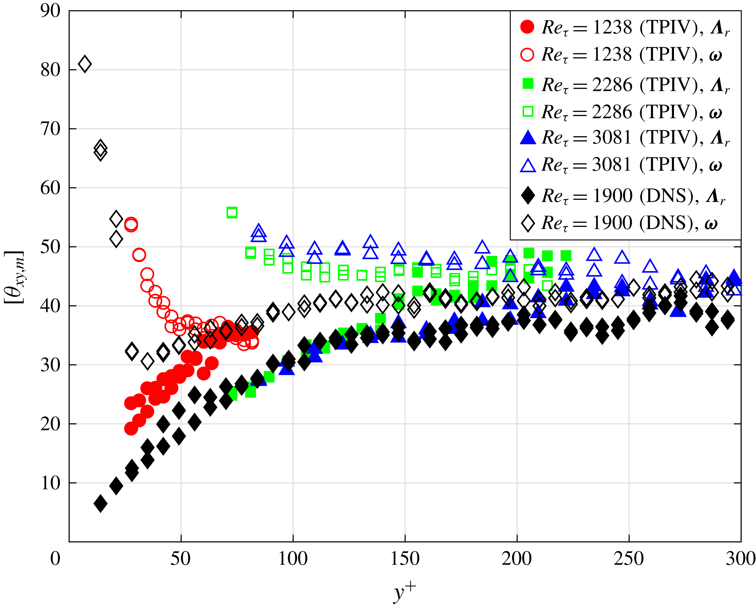
For further comparison between the orientations of
 $\unicode[STIX]{x1D726}_{r}$
and
 $\unicode[STIX]{x1D74E}$
, the most probable inclination angles (
 $\unicode[STIX]{x1D703}_{xy,m}$
or
 $\unicode[STIX]{x1D703}_{-zx,m}$
) could be identified and collected for comparison. For the wall-normal range considered, the p.d.f. curves for
 $\unicode[STIX]{x1D703}_{xy}$
in terms of both
 $\unicode[STIX]{x1D726}_{r}$
and
 $\unicode[STIX]{x1D74E}$
have two obvious local maxima (
 $\unicode[STIX]{x1D703}_{xy,m}$
), which makes it very convenient for identification and comparison. However, the situation is different for the p.d.f.s of
 $\unicode[STIX]{x1D703}_{-zx}$
. While the p.d.f. curve of
 $\unicode[STIX]{x1D703}_{-zx}$
in terms of
 $\unicode[STIX]{x1D726}_{r}$
has two local maxima (
 $\unicode[STIX]{x1D703}_{-zx,m}$
) at the lower normal position (such as
 $y^{+}\approx 50$
shown in figure 8
b), the corresponding p.d.f. curve in terms of
 $\unicode[STIX]{x1D74E}$
has an additional peak at
 $\unicode[STIX]{x1D703}_{-zx}=0$
, which sometimes covers up the other two potential peaks and causes difficulty in the identification (as shown by the red line in figure 10
b). Therefore, only
 $\unicode[STIX]{x1D703}_{xy,m}$
is considered in the following comparison between
 $\unicode[STIX]{x1D726}_{r}$
and
 $\unicode[STIX]{x1D74E}$
.
The wall-normal variation of
 $\unicode[STIX]{x1D703}_{xy,m}$
for
 $\unicode[STIX]{x1D726}_{r}$
and
 $\unicode[STIX]{x1D74E}$
is investigated by collecting the results based on both TPIV data and DNS data as functions of
 $y^{+}$
. To combine the two individuals of
 $\unicode[STIX]{x1D703}_{xy,m}$
at one wall-normal position, the modulo operation is employed in order to make
 $\unicode[STIX]{x1D703}_{xy,m}$
become a single-valued variable ranging from 0 to 90. The modulo operation on
 $\unicode[STIX]{x1D703}_{xy,m}$
is defined as
 $[\unicode[STIX]{x1D703}_{xy,m}]=\text{mod}(\unicode[STIX]{x1D703}_{xy,m},180)$
, with mod(
 $\cdot ,180$
) denoting the modulo operation, returning the remainder after division by 180. The results are shown in figure 11. Still, deviations are observed between the results of TPIV data and DNS data, which are caused by the resolution issue of TPIV data as explained in the following § 3.2.4. Neglecting such deviations, all the results show a consistent trend for the wall-normal variations of
 $\unicode[STIX]{x1D703}_{xy,m}$
. This shows that, for all the Reynolds numbers, the inclination angle for
 $\unicode[STIX]{x1D74E}$
in the
 $x$
–
 $y$
plane is larger than that for
 $\unicode[STIX]{x1D726}_{r}$
and the difference is quite large in the region very close to the wall where the gradient of mean velocity is large, which is consistent with the results in Gao et al. (Reference Gao, Ortizdueñas and Longmire2011). This inclination angle for
 $\unicode[STIX]{x1D726}_{r}$
keeps increasing with the increase of
 $y^{+}$
and its deviation from that of
 $\unicode[STIX]{x1D74E}$
decreases monotonically. At
 $y^{+}=150$
, the two sets of curves for
 $\unicode[STIX]{x1D703}_{xy,m}$
approach each other and begin to level off at
 $40^{\circ }$
–
 $45^{\circ }$
together.
Why do the curves for
 $\unicode[STIX]{x1D703}_{xy,m}$
in terms of both
 $\unicode[STIX]{x1D726}_{r}$
and
 $\unicode[STIX]{x1D74E}$
collapse onto a horizontal line and what does that mean? In a quite early research work, Theodorsen (Reference Theodorsen1952) predicted that the leg of a hairpin vortex should incline at
 $45^{\circ }$
to the streamwise direction. The explanation (Head & Bandyopadhyay Reference Head and Bandyopadhyay1981) came from the governing equation for enstrophy, which takes the form
 $$\begin{eqnarray}\frac{\text{d}e}{\text{d}t}=\unicode[STIX]{x1D74E}\boldsymbol{\cdot }\boldsymbol{S}\boldsymbol{\cdot }\unicode[STIX]{x1D74E}+\unicode[STIX]{x1D708}\,\unicode[STIX]{x1D74E}\boldsymbol{\cdot }\unicode[STIX]{x0394}\unicode[STIX]{x1D74E},\end{eqnarray}$$
where
 $\boldsymbol{S}=(\unicode[STIX]{x1D735}\boldsymbol{u}+\unicode[STIX]{x1D735}^{\text{T}}\boldsymbol{u})/2$
is the rate-of-strain tensor,
 $e=\unicode[STIX]{x1D74E}\boldsymbol{\cdot }\unicode[STIX]{x1D74E}/2$
represents the enstrophy and
 $\unicode[STIX]{x1D708}$
is the kinematic viscosity of the fluid. The first term on the right-hand side of the above equation is the production term of the vorticity, and it indicates that an increasing rate of enstrophy depends on the stretching rate of the material line element along the vorticity direction. When the vorticity is in line with the principal axis of
 $\boldsymbol{S}$
corresponding to the largest eigenvalue, the enstrophy has the largest increasing rate, which means the magnitude of vorticity possesses the largest increasing rate. In a statistical sense,
 $\boldsymbol{S}$
in a TBL corresponds to a pure shear deformation tensor in the
 $x$
–
 $y$
plane because of the TBL mean flow. The corresponding principal axis is along the direction of
 $45^{\circ }$
(Head & Bandyopadhyay Reference Head and Bandyopadhyay1981) inclined to the streamwise direction. Therefore,
 $[\unicode[STIX]{x1D703}_{xy,m}]=45$
corresponds to the direction of vorticity with largest increasing rate in magnitude, which makes the concentration of
 $\unicode[STIX]{x1D74E}$
at
 $[\unicode[STIX]{x1D703}_{xy,m}]=45$
reasonable.
Although the above explanation seems solid, it does not give any clue about the direction of
 $\unicode[STIX]{x1D726}_{r}$
. Considering that
 $\unicode[STIX]{x1D726}_{r}$
has been widely applied in the above sections, further analysis on
 $\unicode[STIX]{x1D726}_{r}$
and its inherent relationship with
 $\unicode[STIX]{x1D74E}$
would create some value for the above work. This time, the investigation departs from the governing equations for vorticity, which is
 $$\begin{eqnarray}\frac{\text{d}\unicode[STIX]{x1D74E}}{\text{d}t}=\boldsymbol{S}\boldsymbol{\cdot }\unicode[STIX]{x1D74E}+\unicode[STIX]{x1D708}\unicode[STIX]{x0394}\unicode[STIX]{x1D74E}.\end{eqnarray}$$
This equation is also equivalent to the following one, noting that
 $\unicode[STIX]{x1D735}\boldsymbol{u}=\boldsymbol{S}+\unicode[STIX]{x1D734}$
and
 $\unicode[STIX]{x1D734}\boldsymbol{\cdot }\unicode[STIX]{x1D74E}=0$
, where
 $\unicode[STIX]{x1D6FA}=(\unicode[STIX]{x1D735}\boldsymbol{u}-\unicode[STIX]{x1D735}^{\text{T}}\boldsymbol{u})/2$
:
 $$\begin{eqnarray}\frac{\text{d}\unicode[STIX]{x1D74E}}{\text{d}t}=\unicode[STIX]{x1D735}\boldsymbol{u}\boldsymbol{\cdot }\unicode[STIX]{x1D74E}+\unicode[STIX]{x1D708}\unicode[STIX]{x0394}\unicode[STIX]{x1D74E}.\end{eqnarray}$$
Still, only the first term on the right-hand side of the equation is focused on in the following analysis, since it is the production term for vorticity.
If a swirl occurs in the locality, i.e.
 $\unicode[STIX]{x1D706}_{ci}>0$
for
 $\unicode[STIX]{x1D735}\boldsymbol{u}$
, then
 $\unicode[STIX]{x1D735}\boldsymbol{u}$
has three different eigenvalues: a real one (
 $\unicode[STIX]{x1D706}_{r}$
), and a pair of conjugated ones. Thus ‘only one’ real eigenvector
 $\unicode[STIX]{x1D726}_{r}$
exists for
 $\unicode[STIX]{x1D735}\boldsymbol{u}$
, satisfying
 $$\begin{eqnarray}\unicode[STIX]{x1D735}\boldsymbol{u}\boldsymbol{\cdot }\unicode[STIX]{x1D726}_{r}=\unicode[STIX]{x1D706}_{r}\unicode[STIX]{x1D726}_{r}.\end{eqnarray}$$
Herein, the term ‘only one’ means kind of unique, in the sense that the direction of
 $\unicode[STIX]{x1D726}_{r}$
is unique while the magnitude might be variable.
If
 $\unicode[STIX]{x1D74E}$
is in line with
 $\unicode[STIX]{x1D726}_{r}$
, i.e.
 $\unicode[STIX]{x1D74E}=c\unicode[STIX]{x1D726}_{r}$
, then
 $$\begin{eqnarray}\unicode[STIX]{x1D735}\boldsymbol{u}\boldsymbol{\cdot }\unicode[STIX]{x1D74E}=\unicode[STIX]{x1D735}\boldsymbol{u}\boldsymbol{\cdot }(c\unicode[STIX]{x1D726}_{r})=c\unicode[STIX]{x1D706}_{r}\unicode[STIX]{x1D726}_{r}=\unicode[STIX]{x1D706}_{r}\unicode[STIX]{x1D74E},\end{eqnarray}$$
where
 $c$
is a constant number.
Considering that the left-hand side of the above equation corresponds to the principal term of vorticity generation, the above equation means that the rate of change for
 $\unicode[STIX]{x1D74E}$
is parallel to
 $\unicode[STIX]{x1D74E}$
itself. Thus, one may conclude that if
 $\unicode[STIX]{x1D74E}$
is in line with
 $\unicode[STIX]{x1D726}_{r}$
,
 $\unicode[STIX]{x1D74E}$
would not change direction in the following small time interval. If not, since the direction of
 $\unicode[STIX]{x1D726}_{r}$
satisfying (3.7) is unique,
 $\unicode[STIX]{x1D74E}$
would change its direction. In other words,
 $\unicode[STIX]{x1D726}_{r}$
provides an important reference to judge whether
 $\unicode[STIX]{x1D74E}$
could keep its orientation, which gives some insight into the inherent relationships between them.
The above conclusion helps in the further discussion about figure 11. At the wall region (
 $y^{+}<100$
), the sharp difference between the orientations of
 $\unicode[STIX]{x1D74E}$
and
 $\unicode[STIX]{x1D726}_{r}$
indicates that
 $\unicode[STIX]{x1D74E}$
would change direction in the following time interval. At the same time, the quasi-streamwise vortex pairs carrying strong
 $\unicode[STIX]{x1D74E}$
are typically elevated by the inducing effect of themselves. Such an elevating motion of
 $\unicode[STIX]{x1D74E}$
accompanied by the changing of its orientation would lead to a wall-normal variation of the orientation of
 $\unicode[STIX]{x1D74E}$
, which can be clearly observed in figure 11. For
 $y^{+}>150$
, when the included angle of
 $\unicode[STIX]{x1D726}_{r}$
and
 $\unicode[STIX]{x1D74E}$
is significantly reduced, the direction of
 $\unicode[STIX]{x1D74E}$
stops changing with
 $y^{+}$
, following the same logic. The inherent relationship between
 $\unicode[STIX]{x1D726}_{r}$
and
 $\unicode[STIX]{x1D74E}$
introduced in this work provides an explanation for the phenomenon displayed in figure 11.
3.2.4 Discussions on Reynolds-number effect and the resolution issue
Although the TPIV data contain three cases with different Reynolds numbers, the corresponding spatial resolutions, which are determined by the interrogation window of the cross-correlation analysis, differ significantly. Such deviations in spatial resolution cause a failure in analysing the Reynolds-number effect on vortex orientations based on TPIV data. To make up for the drawbacks of TPIV data, a further statistical investigation on the DNS data is performed and the results from different Reynolds numbers are quantitatively compared. Figure 12 collects the p.d.f. curves for
 $\unicode[STIX]{x1D703}_{xy}$
and
 $\unicode[STIX]{x1D703}_{-zx}$
in terms of
 $\unicode[STIX]{x1D726}_{r}$
and
 $\unicode[STIX]{x1D74E}$
, and the results based on DNS data with three different Reynolds numbers are compared. It shows that the p.d.f. curves for different Reynolds numbers collapse onto one single curve for a fixed wall-normal position. The results strongly validate that the p.d.f.s of
 $\unicode[STIX]{x1D703}_{xy}$
and
 $\unicode[STIX]{x1D703}_{-zx}$
are independent of Reynolds number. Such a conclusion is consistent with the opinion that the Reynolds number has an obvious influence on large-scale structures while the properties of fine-scale structures (as recognized by the swirl criterion employed here) could be scaled only by the inner scale, independent of the Reynolds number (Hutchins et al.
Reference Hutchins, Nickels, Marusic and Chong2009; Jiménez Reference Jiménez2018).
The p.d.f. curves for
 $\unicode[STIX]{x1D703}_{xy}$
and
 $\unicode[STIX]{x1D703}_{-zx}$
in terms of
 $\unicode[STIX]{x1D726}_{r}$
and
 $\unicode[STIX]{x1D74E}$
at two example wall-normal positions for DNS data with different Reynolds numbers.

In the discussion of §§ 3.2.1 and 3.2.3, the deviations between the results of TPIV data and DNS data are explained as the result of experimental uncertainty and insufficient spatial resolution. While the experimental uncertainty could be reduced by optimizing the experimental configurations or the TPIV processing algorithm, the spatial resolution issue is unavoidable. To make a further investigation on the effect of the spatial resolution issue on the statistical results discussed above, a numerical test on DNS data is performed. In this test, the DNS data for
 $Re_{\unicode[STIX]{x1D70F}}=1900$
are filtered by a 3-D window of
 $33.1\times 33.1\times 33.1$
(wall units), which is consistent with the spatial resolution of TPIV data for
 $Re_{\unicode[STIX]{x1D70F}}=2286$
. The results for the p.d.f. of
 $\unicode[STIX]{x1D703}_{xy}$
and
 $\unicode[STIX]{x1D703}_{-zx}$
based on the original and filtered DNS data are collected in figure 13. At first glance, obvious deviations between the two results can be observed. The p.d.f. peaks for the filtered DNS data are usually higher than the original DNS data. Recalling the discussion of figures 8 and 10, the p.d.f. peaks for the TPIV data, which also suffer from the spatial resolution issue, are lower than that of the DNS data. This seemingly contradictory result could be explained by inherent measurement errors in TPIV data, which is not considered in the above test. For the results of
 $\unicode[STIX]{x1D726}_{r}$
(figure 13
a,c), the filtering effect on DNS data does not obviously change the shapes of the original p.d.f. curves. And the horizontal positions of the corresponding p.d.f. peaks slightly shift away from the original positions. Differently, the results of
 $\unicode[STIX]{x1D74E}$
(figure 13
b,d) are significantly influenced by the filtering effect especially at
 $y^{+}\approx 50$
. In figure 13(b), the filtering effect causes a shift of more than
 $10^{\circ }$
with regard to
 $\unicode[STIX]{x1D703}_{xy,m}$
of
 $\unicode[STIX]{x1D74E}$
at
 $y^{+}\approx 50$
. In figure 13(d), the p.d.f. curve for the filtered data shows a strong peak at
 $\unicode[STIX]{x1D703}_{-zx}=0$
, and the two small humps at
 $\unicode[STIX]{x1D703}_{-zx}\approx \pm 90$
of the original p.d.f. curves are concealed. The influence on the p.d.f. of
 $\unicode[STIX]{x1D703}_{-zx}$
brought by the filtering effect is very consistent with the results of TPIV data when compared to the DNS data. The results shown in figure 13 indicate that
 $\unicode[STIX]{x1D726}_{r}$
is more robust in recognizing the vortex orientations when the data suffer from insufficient spatial resolution, which adds to the value of the
 $\unicode[STIX]{x1D726}_{r}$
criterion.
The p.d.f. for
 $\unicode[STIX]{x1D703}_{xy}$
and
 $\unicode[STIX]{x1D703}_{-zx}$
in terms of
 $\unicode[STIX]{x1D726}_{r}$
and
 $\unicode[STIX]{x1D74E}$
at two example wall-normal positions (
 $y^{+}\approx 50$
and
 $y^{+}\approx 200$
) for original and filtered DNS data of
 $Re_{\unicode[STIX]{x1D70F}}=1900$
.

Vortex structures dominating ejection events at different wall-normal positions. These vortices are recognized from the LSE flow fields by isosurfaces of
 $\unicode[STIX]{x1D706}_{ci}=0.4\unicode[STIX]{x1D706}_{ci,max}$
with colours representing the streamwise velocity fluctuations. The vortices for reference ejection events at different wall-normal positions are arranged along the streamwise direction according to
 $x_{e}^{+}=10y_{e}^{+}$
, where
 $x_{e}^{+}$
and
 $y_{e}^{+}$
are the coordinates of the corresponding ejection events. The vortices from different Reynolds-number cases (including both TPIV data and DNS data) are located at different spanwise positions. Panels (a), (b), (c) and (d) correspond to the top, front, side and oblique views, respectively.

Widths of the LSE vortices (
 $W$
) and their deviations caused by TPIV resolution. (a) Width of the LSE vortices (
 $W$
) as a function of wall-normal position based on the results of TPIV data and DNS data. (b) The deviations of
 $W$
caused by filtering the DNS data according to the interrogation windows of three TPIV configurations. (c) Corrected TPIV results (
 $W$
) based on the corresponding deviations in (b) compared with the DNS results of
 $Re_{\unicode[STIX]{x1D70F}}=1900$
.

3.3 Extracting dominant structures by LSE
In § 3.2, the vortex orientation has been statistically investigated by using
 $\unicode[STIX]{x1D726}_{r}$
, which reflects the local features of the vortex structures in a TBL. In this section, as a necessary supplement for the above investigations, we focus on the global features of vortex structures in spatial organization. As introduced in § 2, the LSE method will be employed to directly extract complete structures from TBL fields, which reflects the overall characteristics of vortex structures in spatial organization associated with the given LSE events.
3.3.1 LSE for an ejection event
Figure 14 displays the vortex structures identified from the LSE flow fields given ejection events at different wall-normal positions. These LSE vortices are well collected into one coordinate system, with corresponding reference event arranged along an inclined line
 $x_{e}^{+}=10y_{e}^{+}$
. Therefore, the variation of vortex shapes along the
 $x$
axis reflects the wall-normal evolution of LSE structure. For better comparison, the LSE vortices resulting from different Reynolds numbers are arranged at different spanwise positions, as indicated by the annotations on the right side of figure 14(a). It shows that, for
 $y^{+}<40$
(corresponding to
 $x^{+}<400$
in the figure), the dominant structure for an ejection event is a pair of counter-rotated streamwise vortices, with a spanwise spacing of 50–100 wall units. A weak spanwise vortex tube connects the streamwise vortex pair, forming an ‘H’-shaped vortex. With the increase of wall-normal distances, the angle of inclination to the streamwise direction for the ‘H’ vortex continuously increases until
 $y^{+}=120$
, from which the inclination angle keeps constant at approximately
 $45^{\circ }$
. Such a wall-normal evolution trend for the inclination angle is consistent with the results in § 3.2. The parallel and streamwise-extending parts downstream of the connection position shrink to become small tongue-like protuberances, which is the remnant of the vortex transition process and has also been observed by Jodai & Elsinga (Reference Jodai and Elsinga2016) in an instantaneous field. When the spanwise vortex becomes stronger, the LSE structure transforms from ‘H’ vortex into a typical hairpin, which finishes at approximately
 $y^{+}=60$
. At
 $y^{+}>100$
, a second spanwise vortex occurs between the two legs, which rotates in the opposite direction to the former spanwise vortex. Together, the two spanwise vortex tubes and the two bordering legs form a structure with a loop-like head. The loop-like vortex is the conditional vortex of an isotropic turbulence (Adrian Reference Adrian1979), whose occurrence indicates that the local flow is close to isotropic turbulence and the logarithmic region has begun. The structures continuously increase with the wall-normal positions while keeping the characteristic shape unchanged. The results from different Reynolds numbers show very good consistency in the topological shapes. For the TPIV data of
 $Re_{\unicode[STIX]{x1D70F}}=3081$
, the vortices appear somewhat fatter than the ones from DNS data, which is caused by the comparatively lower spatial resolution of these TPIV data.
To quantitatively investigate the size evolution of LSE structures, the characteristic width
 $W$
is defined as follows. First, the swirl strength (
 $\unicode[STIX]{x1D706}_{ci}$
) distribution in the slice at the height of the reference ejection event is extracted. Then, the two maximum peaks on the slice are recognized and their spanwise distance is calculated, which is defined as the width of LSE structures
 $W$
. Figure 15(a) shows
 $W$
as a function of wall-normal position for all the Reynolds numbers. It shows that the widths increase with
 $y^{+}$
and the increasing speed becomes stable when
 $y^{+}>100$
. The linear increasing trend of vortex size is consistent with the famous attached eddy hypothesis, which is an important theory accurately predicting the statistics of the log region (Woodcock & Marusic Reference Woodcock and Marusic2015). For the DNS data,
 $W$
from three different Reynolds numbers collapse onto a single curve, which indicates that the widths of vortex structures are independent of Reynolds number. For the TPIV data, the curves for three Reynolds numbers appear parallel and could be well overlapped only by shifting a constant distance along the vertical direction. Such constant shift might be caused by the variance of TPIV resolution for different Reynolds numbers, which has been noticed in the discussion of figure 14.
To estimate the deviations of
 $W$
caused by the resolution issue, another numerical test is performed on the DNS data of
 $Re_{\unicode[STIX]{x1D70F}}=1900$
. This time, the DNS data are filtered by the three interrogation windows corresponding to the three cases of TPIV data, which have been listed in table 1. Then
 $W$
calculated from the filtered DNS data are compared to
 $W$
based on the original DNS data. The corresponding deviations (denoted as
 $\unicode[STIX]{x0394}W$
) are shown in figure 15 as functions of wall-normal positions. It shows that
 $\unicode[STIX]{x0394}W$
approximately remains constant for
 $y^{+}>100$
, and increases with the size of the filter window. Such variations of
 $\unicode[STIX]{x0394}W$
with different wall-normal positions and filtering windows are consistent with the deviations of the TPIV results when comparing to the DNS data as shown in figure 15(a). Therefore, the results of
 $\unicode[STIX]{x0394}W$
in the numerical test are employed to correct the TPIV results in figure 15(a), accordingly. The final results depicted in figure 15(c) show that the corrected TPIV data are close to the DNS data, which validates the consistency of TPIV data and DNS data.
Spanwise vorticity distribution in
 $x$
–
 $y$
planes extracted from the LSE flow fields given a centred prograde spanwise vortex. Panels (a) and (b) correspond to the results of DNS data for
 $Re_{\unicode[STIX]{x1D70F}}=1100$
and
 $Re_{\unicode[STIX]{x1D70F}}=1900$
. Panel (c) corresponds to a combination of the TPIV results for
 $Re_{\unicode[STIX]{x1D70F}}=1238$
,
 $Re_{\unicode[STIX]{x1D70F}}=2286$
and
 $Re_{\unicode[STIX]{x1D70F}}=3081$
. The contour maps in the three columns show the results estimated based on the conditional spanwise vortices at three different wall-normal positions, as illustrated in the corresponding headings.

3.3.2 LSE for a prograde spanwise vortex
Figure 16 displays the spanwise vorticity distribution in the
 $x$
–
 $y$
plane extracted from LSE flow fields given a centred prograde spanwise vortex. The results based on two sets of DNS data for
 $Re_{\unicode[STIX]{x1D70F}}=1100$
and
 $Re_{\unicode[STIX]{x1D70F}}=1900$
are provided in the first two rows. For each Reynolds-number case, three example wall-normal positions of
 $y^{+}=63.0$
,
 $y^{+}=161.0$
and
 $y^{+}=210.0$
are chosen as the position of centred spanwise vortex, and the corresponding results are displayed in the three columns. For TPIV data, since the three cases with different Reynolds numbers have limited wall-normal range, only one LSE field for each case is displayed. The TPIV results are combined to display in the third row of figure 16. At lower wall-normal positions (as shown in figure 16
a1,b1,c1), the contour shows one strong central vortex and two inclined shear layers located upstream and downstream of the centred vortex. When the central vortices depart from the wall, the inclination angles for the shear layers increase. In figure 16(a2,b2,c2), obvious vorticity peaks occur on the upstream and downstream shear layers. The occurrence of the vorticity peaks makes the structure quite resemble a typical packet structure, which contains the head parts of several hairpins distributing on an inclined shear layer. Farther away from the wall, the vorticity peaks become weak but are still distinguishable as shown in figure 16(b3,c3). According to the DNS data, the spacing between the central vortex and its neighbouring upstream one is estimated to be 175 wall units for
 $Re_{\unicode[STIX]{x1D70F}}=1100$
and 200 wall units for
 $Re_{\unicode[STIX]{x1D70F}}=1900$
. The spacing remains almost constant with the increase of wall-normal position, but becomes larger with the increase of the Reynolds number. When comparing the results of TPIV data and DNS data, one obvious difference is observed in the neighbouring region of the central vortex. Two small vorticity peaks occur in this region for TPIV data, between which the central vortex is sandwiched along an approximately horizontal line. This awkward vorticity distribution occurs in all the three cases of TPIV data, as marked by the magenta arrows in figure 16. In both figure 16(c2,c3), imagining that the two small vorticity peaks are razed and the gap between either of them and the central vortex is filled, the resulting vorticity distribution would be quite similar to the DNS results (figure 16
b2,b3). Based on these observations, the authors believe that the two small vorticity peaks are caused by measurement uncertainties, which contribute to the interruption of vorticity in the locality. Once accepting that, the results of TPIV data and DNS data would be remarkably consistent as the dashed magenta circles indicated. Anyway, these current results provide statistical proofs for the packet structures and cast some light on their geometric characteristics.
Statistical evidence for hairpin packets was first provided by Christensen & Adrian (Reference Christensen and Adrian2001), who found an inclined shear layer in LSE velocity field based on 2-D PIV data (in the
 $x$
–
 $y$
plane). The shear layer was recognized by using the map of unit vectors, and irregular spanwise vortices were discovered on the shear layer. Recently, Deng et al. (Reference Deng, Pan, Wang and He2018) designed a proper orthogonal decomposition-based filter technique, and tried to filter out the isolated vortices before performing self-correlation on the 2-D
 $\unicode[STIX]{x1D706}_{ci}$
field (in the
 $x$
–
 $y$
plane). They found three peaks aligned along an inclined line, which corresponds to three spanwise vortices in one packet structure. In this work, without an extra filter operation, the LSE technique could provide a multi-peak pattern in the
 $x$
–
 $y$
plane, which is attributed to the advantage of 3-D velocity data. The volumetric data support a spanwise average in the calculation of LSE velocity field, which would strengthen the effects of spanwise vortices, as most of them extend along the spanwise direction. The success of extracting hairpin packets from 3-D velocity data could provoke more interest in the analysis on 3-D TBL data.
3.4 Further discussions
While § 3.1 discussed the characteristics of typical vortices and their spatial organization in an instantaneous TBL flow, §§ 3.2 and 3.3 extended the discussion by quantifying the probability for the occurrence of the typical structure and depicting its geometry in a statistical sense. These results in §§ 3.1 and 3.3 cooperatively sketch out a picture for the vortex structures and their evolution below the logarithmic regions of TBLs. The buffer region is populated by quasi-streamwise vortices, which usually occur in pairs and are distributed along meandering low-speed streaks as shown in figure 5. The quasi-streamwise vortices suffer from strong shear flows, which results in significant differences in the orientations of local vorticity and swirl. The quasi-streamwise vortices usually bend away from the wall and turn towards the spanwise direction when they extend downstream. This characteristic could either be observed from the instantaneous field, or be inferred based on the wall-normal variations of the p.d.f.s for
 $\unicode[STIX]{x1D703}_{xy}$
and
 $\unicode[STIX]{x1D703}_{-zx}$
. On the top of the low-speed streaks, these streamwise vortices interact with the neighbouring ones and form complex structures such as hairpin vortices or arc vortices, which contribute to the plateau of the p.d.f. curves for
 $\unicode[STIX]{x1D703}_{-zx}$
. The vortex structure with tongue-like protrusions found in the LSE results (figure 14) also indicates that the hairpin structure could be evolved from a pair of streamwise vortices. In the logarithmic region, when the interaction effect between vortices becomes weaker, the dominant vortex structures from different wall-normal positions keep similar geometries. The ejection event in this region is dominated by a hairpin structure, which is inclined at
 $45^{\circ }$
along the streamwise direction and possesses a loop-like head. The width of the hairpin structure increases linearly with the wall-normal position, supporting the famous attached eddy hypothesis.
When an incoming sweep event is blocked by the ejection event induced by an existed hairpin structure, a spanwise vortex would occur by the rolling-up effect. If the newly formed spanwise vortex is connected to the legs of the existing hairpin structure, a typical packet structure would form. In a TBL, the incoming sweep event could be produced by the inducing effect of an upstream spanwise vortex, which is abundant in the logarithmic region as shown by the p.d.f. of
 $\unicode[STIX]{x1D703}_{-zx}$
. The packet structures composed of several spanwise vortices also exist in the logarithmic region, which promote the momentum exchange of TBLs at large scales. Results from this work support the classical opinions about the schematics of vortex structures in TBLs (Robinson Reference Robinson1991; Adrian Reference Adrian2007), yet providing more proofs and details about the structures and their wall-normal evolutions.
4 Concluding remarks
Tomographic PIV measurements are conducted to capture the vortex structures below
 $y/\unicode[STIX]{x1D6FF}=0.1$
for three Reynolds numbers from
 $Re_{\unicode[STIX]{x1D70F}}=1238$
to
 $Re_{\unicode[STIX]{x1D70F}}=3081$
. Results of the TPIV measurements combined with the DNS results are analysed, which provides plenty of information about the vortex structures below the logarithmic region.
The instantaneous velocity field from TPIV results shows typical vortex structures in the buffer region. Quasi-streamwise vortices with various scales and shapes are distributed around several streamwise-extending low-speed streaks. A hairpin-like structure is formed by the connection of a pair of quasi-streamwise vortices from the two sides of one low-speed streak, which is consistent with the observation of Jodai & Elsinga (Reference Jodai and Elsinga2016). A vortex group containing a typical hairpin vortex and three spanwise vortices upstream is observed, which shows a typical packet signature in the
 $x$
–
 $y$
plane.
The vortex orientation is quantitatively investigated by using the real eigenvector of the velocity gradient tensor. The p.d.f.s of
 $\unicode[STIX]{x1D703}_{xy}$
show two local maxima for the wall-normal range considered, which are named as the most probable inclination angle (
 $\unicode[STIX]{x1D703}_{xy,m}$
). With the increase of wall-normal distance,
 $\unicode[STIX]{x1D703}_{xy,m}$
continuously increases and levels off at approximately
 $45^{\circ }$
and
 $-135^{\circ }$
, which are correlated with the two legs of the hairpin structures. The p.d.f. of
 $\unicode[STIX]{x1D703}_{-zx}$
also shows two maximum peaks at
 $\pm 60^{\circ }$
–
 $70^{\circ }$
for
 $y^{+}<100$
. For higher wall-normal position, the two maximum peaks become less prominent and the corresponding
 $\unicode[STIX]{x1D703}_{-zx}$
(
 $\unicode[STIX]{x1D703}_{-zx,m}$
) tend to approach
 $\unicode[STIX]{x1D703}_{-zx}=0$
(spanwise direction). Based on the quantitative results about the most probable orientations, a sketch of the imaginary vortex tube is provided. The conceptual vortex tube bends upwards and changes direction from the streamwise towards the spanwise with the increase of wall-normal position, resembling some vortex structures observed in the instantaneous field.
The orientation of vorticity is also statistically investigated by the p.d.f.s of the corresponding
 $\unicode[STIX]{x1D703}_{xy}$
and
 $\unicode[STIX]{x1D703}_{-zx}$
. Results indicate that the orientation of
 $\unicode[STIX]{x1D74E}$
is significantly influenced by the mean shear flow of the TBL. The
 $\unicode[STIX]{x1D703}_{xy,m}$
in terms of
 $\unicode[STIX]{x1D74E}$
is larger than that of
 $\unicode[STIX]{x1D726}_{r}$
, but the difference becomes small with the increase of wall-normal position. The inherent relationship between the orientations of
 $\unicode[STIX]{x1D726}_{r}$
and
 $\unicode[STIX]{x1D74E}$
is analysed by using the governing equation of vorticity. It shows that
 $\unicode[STIX]{x1D726}_{r}$
provides an important reference to judge whether
 $\unicode[STIX]{x1D74E}$
could keep its orientation.
The LSE velocity fields given ejection events happening at different wall-normal positions shed some light on the evolution of the vortices dominating the ejection events. A transition from streamwise vortex to hairpin vortex is observed when the ejection event leaves away from the wall, consistent with variation of
 $\unicode[STIX]{x1D703}_{xy,m}$
and
 $\unicode[STIX]{x1D703}_{-zx,m}$
discussed before. At
 $y^{+}=50$
, a vortex structure with two tongue-like bulges is observed, which could be viewed as the remnant of this transition process. The LSE vortex with a loop-like head occurs at approximately
 $y^{+}=120$
, indicating the mature hairpin vortex and also the start of the logarithmic region. Further away from the wall, the shape of the LSE vortex remains similar while its width increases at a constant rate, which validates the famous attached eddy hypothesis.
An LSE based on a centred prograde spanwise vortex results in a typical packet signature in the
 $x$
–
 $y$
plane. The inclination angle with respect to the wall for the packets increases when they depart away from the wall. The streamwise spacing for the neighbouring hairpin heads is estimated as 150–200 wall units for the Reynolds-number range considered. The spacing stays nearly constant with the increase of wall-normal position, but becomes larger with the increase of the Reynolds number. The results based on TPIV data and DNS data agree well in this work, which provides credible evidence for the existence of packet structures.
In this work, the deviations between TPIV results and DNS results are noticed and analysed carefully. The influence of Reynolds number is excluded by comparing the DNS results for different Reynolds numbers. Therefore, these deviations are caused by the measurement uncertainties and the resolution issue of TPIV results. Numerical tests on the DNS data are performed to quantify the influence of this resolution problem. Results of the tests explain some aspects of the deviations in these p.d.f. curves based on TPIV data and DNS data. The orientation of
 $\unicode[STIX]{x1D726}_{r}$
is more robust to the resolution issue compared to the orientation of
 $\unicode[STIX]{x1D74E}$
, which adds some value to the
 $\unicode[STIX]{x1D726}_{r}$
criterion. The tests also provide a solution to correct the width of LSE vortex suffering from the resolution issue, which works well on the TPIV data. The numerical tests and the comparison between TPIV results and DNS results are a reminder that the influence of the resolution issue should be considered when carrying out a similar analysis based on PIV or TPIV data.
Acknowledgements
This work was supported by the National Natural Science Foundation of China (grant nos 11490552, 11721202) and the Fundamental Research Funds for the Central Universities (2019QNA4056).



