1 Introduction
1.1 Background and motivation
The impact of millimetre-sized objects on surfaces has been investigated in great detail. Examples are the study of single drop impact onto a liquid pool (Pumphrey & Elmore Reference Pumphrey and Elmore1990; Prosperetti & Oguz Reference Prosperetti and Oguz1993; Thoroddsen et al.
Reference Thoroddsen, Thoraval, Takehara and Etoh2012; Tran et al.
Reference Tran, de Maldeprade, Sun and Lohse2013; Wang, Kuan & Tsai Reference Wang, Kuan and Tsai2013; Chen & Guo Reference Chen and Guo2014; Hendrix et al.
Reference Hendrix, Bouwhuis, van der Meer, Lohse and Snoeijer2016) (focusing on typical terminal velocities of order
 $1~\text{m s}^{-1}$
), multiple drop impact on a pool (Bick et al.
Reference Bick, Ristenpart, van Nierop and Stone2010) or the impact of a solid object onto a pool (Bergmann et al.
Reference Bergmann, van der Meer, Stijnman, Sandtke, Prosperetti and Lohse2006; Gekle et al.
Reference Gekle, van der Bos, Bergmann, van der Meer and Lohse2008; Bergmann et al.
Reference Bergmann, van der Meer, Gekle, van der Bos and Lohse2009; Gekle et al.
Reference Gekle, Snoeijer, Lohse and van der Meer2009, Reference Gekle, Peters, Gordillo, van der Meer and Lohse2010). Another example is the impact of a continuous water mass, thus a liquid column or a jet, onto a pool (Kolaini et al.
Reference Kolaini, Roy, Crum and Mao1993; Oguz, Prosperetti & Kolaini Reference Oguz, Prosperetti and Kolaini1995; Clanet & Lasheras Reference Clanet and Lasheras1997; Storr & Behnia Reference Storr and Behnia1999; Kersten, Ohl & Prosperetti Reference Kersten, Ohl and Prosperetti2003; Szymczak, Means & Rogers Reference Szymczak, Means and Rogers2004; Qu et al.
Reference Qu, Khezzar, Danciu, Labois and Lakehal2011). These studies focused on the bubbles resulting from the hydrostatic collapse of the generated cavity. Only recently has the focus shifted to the impact of much smaller drops, with a radius of a few tens of micrometres, corresponding to the typical size of drops coming from, e.g., an inkjet nozzle (Basaran, Gao & Bhat Reference Basaran, Gao and Bhat2013; Driessen et al.
Reference Driessen, Jeurissen, Wijshoff, Toschi and Lohse2013). Microdrop impact is highly relevant for many rapidly developing applications, such as immersion lithography (Keij et al.
Reference Keij, Winkels, Castelijns, Riepen and Snoeijer2013), extreme ultraviolet (EUV) lithography (Klein et al.
Reference Klein, Bouwhuis, Visser, Lhuissier, Sun, Snoeijer, Villermaux, Lohse and Gelderblom2015) and 3D printing (Gibson, Rosen & Stucker Reference Gibson, Rosen and Stucker2010; Pohl et al.
Reference Pohl, Visser, Römer, Lohse, Sun and Huis in ’t Veld2015), spray painting and spray coating. Very recently it has been found that the phenomena for microdrops impacting on a solid surface are similar to those of larger (millimetre-sized) impacting drops (Visser et al.
Reference Visser, Frommhold, Wildeman, Mettin, Lohse and Sun2015). In contrast, for impact on a pool on these small length scales, capillary effects are expected to be much more significant when compared to the impact of millimetre-sized drops, or even dominating over gravity (Aristoff & Bush Reference Aristoff and Bush2009). Capillary effects on the small air bubbles resulting from the air-film rupture have been investigated (Bouwhuis et al.
Reference Bouwhuis, van der Veen, Tran, Keij, Winkels, Peters, van der Meer, Sun, Snoeijer and Lohse2012; Lee et al.
Reference Lee, Weon, Je and Fezzaa2012; Bouwhuis et al.
Reference Bouwhuis, Hendrix, van der Meer and Snoeijer2015; Hendrix et al.
Reference Hendrix, Bouwhuis, van der Meer, Lohse and Snoeijer2016), but air bubbles due to the collision of surface waves within the cavity (called ‘regular bubble entrapment’, as described in Pumphrey & Elmore (Reference Pumphrey and Elmore1990), Prosperetti & Oguz (Reference Prosperetti and Oguz1993), Wang et al. (Reference Wang, Kuan and Tsai2013), Chen & Guo (Reference Chen and Guo2014) for millimetre-sized drops) for single impacting microdrops is still ongoing research. Impacting microjets and microdrop trains on liquid pools have not yet been studied in detail.
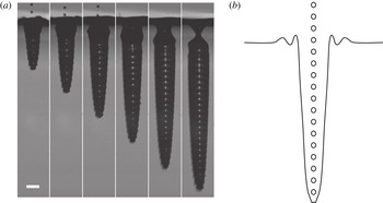
In this paper, we will look at the impact of a high-speed train of uniformly distributed microdrops on a deep liquid pool. In general, the high-energy impact onto a pool creates a deep cavity (figure 1 a). We will focus on the shape and collapse of the cavities as a function of the relevant impact parameters (drop size, velocity, frequency). By performing boundary integral (BI) simulations, where we treat the liquid within the pool and within the impacting drop as potential flow (Gekle et al. Reference Gekle, Peters, Gordillo, van der Meer and Lohse2010; Bouwhuis et al. Reference Bouwhuis, van der Veen, Tran, Keij, Winkels, Peters, van der Meer, Sun, Snoeijer and Lohse2012), the independent modification of these parameters is much more easy than in the experiments (see § 1.2). We subsequently connect the numerical results to simple theoretical analysis from which we deduce scaling laws, revealing the key features of the cavity dynamics. Our work thus forms a major step towards understanding multiple drop impact, which plays a role in all the industrial applications mentioned above.
1.2 Experiments: the creation and impact of a high-velocity microdrop train
Here we briefly describe the experiments reported in figure 1. More details of the set-up can be found in Lindblad & Schneider (Reference Lindblad and Schneider1965), Brenn (Reference Brenn2000), Kim, Park & Min (Reference Kim, Park and Min2003), Frommhold et al. (Reference Frommhold, Lippert, Holsteyns and Mettin2014) and Visser et al. (Reference Visser, Frommhold, Wildeman, Mettin, Lohse and Sun2015). A monodisperse train of droplets is generated at the exit of
 $20~{\rm\mu}\text{m}$
diameter nozzle brought into mild vibrations with a piezoceramic transducer. The nozzle is fed from a reservoir filled with deionized water and pressurized at 5–20 bar using a nitrogen bottle. Applying about 70 V at 100–400 kHz to the transducer perturbs the thin jet exiting the nozzle and leads to its regular break up due to a Rayleigh–Plateau instability. Figure 1(a) shows an experimental result for a frequency of 290 kHz, which gives a temporal droplet spacing of
 ${\sim}3.5~{\rm\mu}\text{s}$
, a velocity of
 ${\sim}30~\text{m s}^{-1}$
and a diameter of
 ${\sim}40~{\rm\mu}\text{m}$
. The length of the train (number of drops) can be controlled by two electric fields. Briefly, the droplet train first passes through a metallic aperture. By applying a short burst of 800 V, individual and multiple droplets can be charged. Then the droplets pass through a pair of deflection plates, which is held at a constant electric field of
 ${\sim}1.5~\text{MV}~\text{m}^{-1}$
. The undeflected/uncharged droplets are collected, while the deflected droplets pass and impact onto the pool.
(a) Experimental snapshots of a cavity created by a train of
 ${\sim}40~{\rm\mu}\text{m}$
diameter water drops, which impact with
 ${\sim}30~\text{m s}^{-1}$
on a deep pool of water. The scale bar is
 $200~{\rm\mu}\text{m}$
, and the interframe time is
 $40~{\rm\mu}\text{s}$
. The cavity reaches a depth of the order of 1000 times the size of a single drop. (b) Sketch of the impacting train of microdrops.

In the experimental time sequence of figure 1(a), one recognizes the typical deep and narrow cavity shape, on top of which one can discern a wavy pattern at the lower end of the cavity, caused by the subsequent impact of the individual drops, as indicated in the sketch of the phenomenon provided in figure 1(b). The downward growth speed of the cavity is approximately constant during the impact of the drop train. The collapse of the cavity typically occurs at the top, near the pool surface.
1.3 Objectives
This paper will focus on several key questions: What is the shape of the cavity and does there exist a similarity profile? What is the dominant collapse mechanism and what is the depth of the cavity at the time of its collapse? Finally, we will demonstrate the role played by the drop frequency and spacing in the answers to these questions.
The paper is structured as follows. In § 2, we will introduce the problem, the assumptions we make in the simulations and in our theoretical modeling, as well as some details of the numerical method. In § 3, we discuss the results of our simulations, and develop a scaling theory to account for these results. Finally, in § 4, we conclude, discuss the limitations of our predictions and give suggestions for future work.
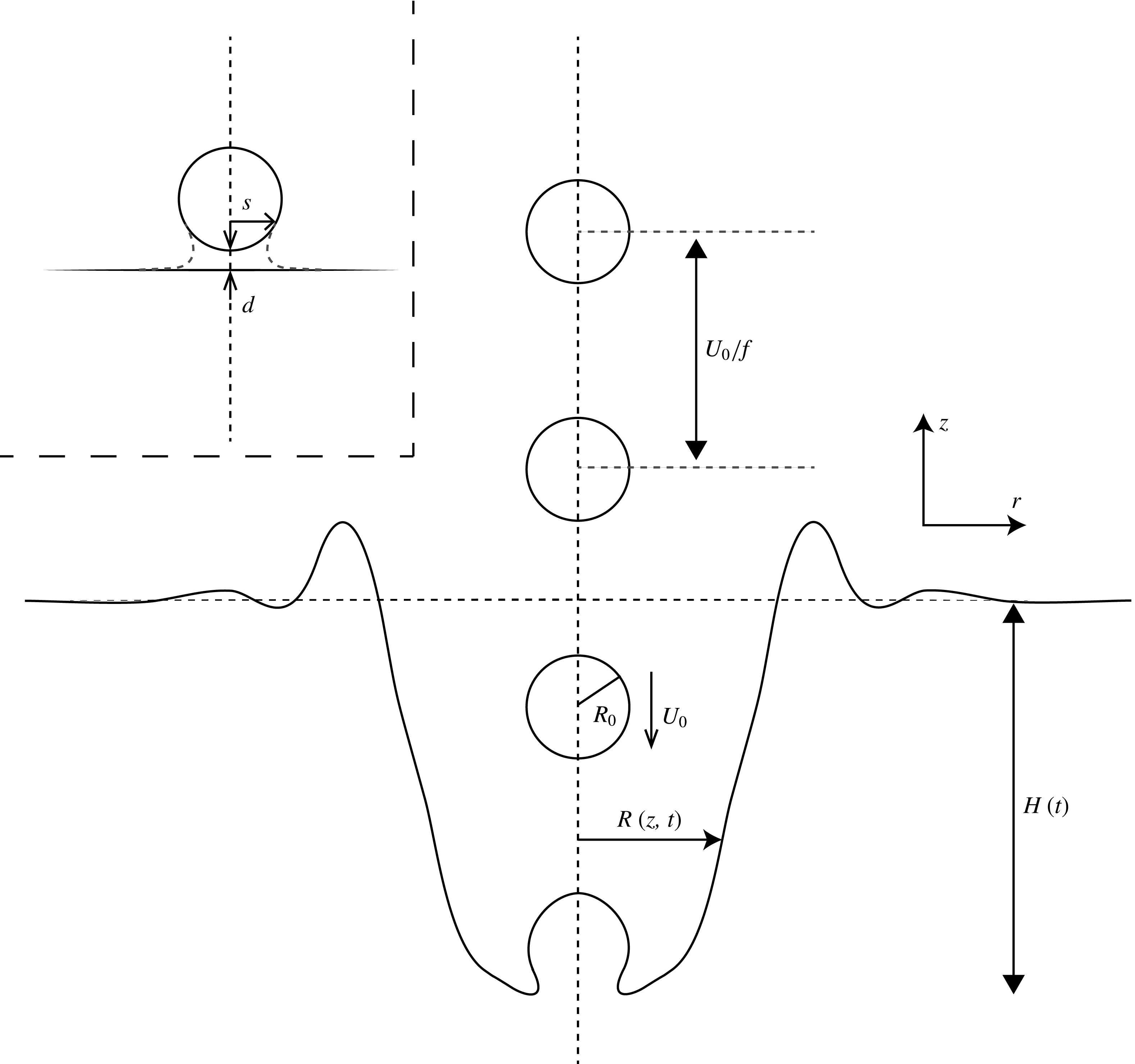
Definition sketch of the parameters. The drop train that consists of drops with radius
 $R_{0}$
and downward velocity
 $U_{0}$
impacts vertically on a pool surface (
 $z=0$
). The drop frequency is
 $f$
and the distance between the drops is
 $U_{0}/f$
. The resulting cavity has a width
 $R(z,t)$
and a depth
 $H(t)$
, where
 $t$
is the time from the first impact. We assume axisymmetry. Inset: numerical recombination; at the instant at which the minimum gap height between the pool and the drop surface becomes a distance
 $d$
, we recombine the drop surface and the pool surface by connecting the pool curve and the drop curve on a radial distance
 $s$
.

2 Problem statement and numerical method
In this section, we formulate the problem and conduct a parameter analysis for the typical orders of magnitude in the experiments described in the introduction (§ 2.1) and show the numerical method (§ 2.2).
2.1 Parameters and assumptions
The geometry of the problem is sketched in figure 2. We assume cylindrical coordinates (
 $r,z$
), with the unit vector
 $\boldsymbol{e}_{z}$
pointing upwards and
 $z=0$
located at the undisturbed surface. In the numerical simulations and in our theoretical analysis we will assume a monodisperse axisymmetric drop train which consists of drops falling down at a frequency
 $f$
. The drops have radius
 $R_{0}$
and velocity
 $U_{0}$
, and impact on an initially quiescent pool surface. The liquid of both the pool and the drops is water, with density
 ${\it\rho}=998.1~\text{kg m}^{-3}$
and air–liquid surface tension
 ${\it\gamma}=72.8~\text{mN m}^{-1}$
. The multiple drop impact on the pool results into a cavity with a time-dependent central depth
 $H(t)$
, where
 $t$
is the time from the first impact (
 $H(0)=0$
). The depth- and time-dependent radius of the cavity is
 $R(z,t)$
.
We can express the control parameters in dimensionless form as the Weber number
 $\mathit{We}={\it\rho}R_{0}U_{0}^{2}/{\it\gamma}$
and the ratio
 $\widetilde{f}$
between the drop diameter
 $2R_{0}$
and the centre-to-centre spacing
 $U_{0}/f$
in between successive drops, i.e.
 $\widetilde{f}=2fR_{0}/U_{0}$
. The limit
 $\widetilde{f}\rightarrow 0$
is the limit of ‘successive’ single-drop impacts: in this limit, the cavity will fully collapse and the pool surface will re-equilibrate and become flat again, before the next drop impacts. The other limit is
 $\widetilde{f}\rightarrow 1$
, which is the theoretical maximum frequency (if
 $\widetilde{f}>1$
, the drops would overlap). In the limit
 $\widetilde{f}=1$
, the supply of downward momentum onto the pool is continuous, which is reminiscent of an impacting jet. One could also call
 $\widetilde{f}$
a Strouhal number, comparing the time needed for the drop to move over its own diameter and the time between two subsequent impacts. In the experiments,
 $\widetilde{f}$
is of course smaller than 1, but still typically of order 1; the spacing between the drops is approximately equal to the drop size.
Further important dimensionless parameters of the system are the Reynolds number of the liquid,
 $\mathit{Re}={\it\rho}R_{0}U_{0}/{\it\eta}$
(where
 ${\it\eta}$
is the dynamic viscosity of the liquid), which is of order 1000 and the Bond number
 $\mathit{Bo}={\it\rho}gR_{0}^{2}/{\it\gamma}$
(where
 $g$
is the acceleration by gravity), which is of order
 $10^{-3}$
. This implies, respectively, that the viscosity of the liquid can be neglected, and that the effect of surface tension dominates over the effect of gravity. The latter should be contrasted to the plunging disks studied in Bergmann et al. (Reference Bergmann, van der Meer, Stijnman, Sandtke, Prosperetti and Lohse2006), Gekle et al. (Reference Gekle, van der Bos, Bergmann, van der Meer and Lohse2008, Reference Gekle, Snoeijer, Lohse and van der Meer2009, Reference Gekle, Peters, Gordillo, van der Meer and Lohse2010), Bergmann et al. (Reference Bergmann, van der Meer, Gekle, van der Bos and Lohse2009) and the impacting water masses studied in Oguz et al. (Reference Oguz, Prosperetti and Kolaini1995), where the collapse of the cavity was mainly determined by the hydrostatic pressure. One can also express the effect of gravity in terms of the Froude number
 $\mathit{Fr}=U_{0}^{2}/(gR_{0})$
. Typically we have
 $\mathit{Fr}\sim 10^{5}$
, such that we can neglect the effect of gravity during the trajectory of the drops. Since the Reynolds number, the Froude number and the Weber number are all much larger than 1, we conclude that the behaviour of the cavity is mainly determined by inertial effects: the cavity collapse occurs at large times. The cavities created by microdrop train impact can thus indeed grow enormously deep, relative to the size of the drops.
Although the Bond number of a single impacting drop may be small, the Bond number based on the length scale of a deep cavity,
 $\mathit{Bo}^{\prime }={\it\rho}gR_{0}H/{\it\gamma}$
, will be much larger, such that the hydrostatic pressure becomes non-negligible at the latter stages of the cavity development (Aristoff & Bush Reference Aristoff and Bush2009). A hydrostatic collapse is a ‘deep collapse’, in the sense that the cavity walls touch the symmetry-axis far below the surface of the pool: a mechanism completely different from a surface-tension-driven cavity collapse. In our analysis, we will at first instance neglect the effect of hydrostatics, because the collapse of the cavity will be initiated by surface tension, as concluded from the above dimensional analysis, which determines the time scales of the collapse. Note that in the BI simulations, we can easily switch on and off the effect of hydrostatics, which is how we confirmed these statements.
We do not simulate the airflow inside the cavity resulting from the movement of both the drop train and the cavity walls. This implies, first, that we neglect any small bubble entrapment caused by the increased gas pressure between the pool and the lowest drop, which is a valid assumption, as the length scale of the air bubble entrapment is much smaller than the drop size (Bouwhuis et al. Reference Bouwhuis, van der Veen, Tran, Keij, Winkels, Peters, van der Meer, Sun, Snoeijer and Lohse2012, Reference Bouwhuis, Hendrix, van der Meer and Snoeijer2015; Hendrix et al. Reference Hendrix, Bouwhuis, van der Meer, Lohse and Snoeijer2016) and will not influence the flow dynamics on the length scale of the cavity. Second, the neglect of the airflow implies that the spherical drops within the train all fall down undecelerated and undeformed (as depicted in figure 2). It appeared from the experiments that this is a reasonable assumption to implement, except for at the beginning and the end of the drop train. We will come back to these effects at § 3.1.
2.2 Numerical method
2.2.1 BI simulations
The liquid within the pool is treated as incompressible, irrotational and inviscid. The Laplace equation,
 ${\rm\nabla}^{2}{\it\phi}=0$
, for the flow potential
 ${\it\phi}$
, is solved along the liquid interface, using the axisymmetric BI method (Oguz & Prosperetti Reference Oguz and Prosperetti1993; Oguz et al.
Reference Oguz, Prosperetti and Kolaini1995; Pozrikidis Reference Pozrikidis1997; Bergmann et al.
Reference Bergmann, van der Meer, Gekle, van der Bos and Lohse2009; Gekle et al.
Reference Gekle, Peters, Gordillo, van der Meer and Lohse2010; Bouwhuis et al.
Reference Bouwhuis, van der Veen, Tran, Keij, Winkels, Peters, van der Meer, Sun, Snoeijer and Lohse2012, Reference Bouwhuis, Winkels, Peters, Brunet, van der Meer and Snoeijer2013, Reference Bouwhuis, Hendrix, van der Meer and Snoeijer2015; Hendrix et al.
Reference Hendrix, Bouwhuis, van der Meer, Lohse and Snoeijer2016). The dynamic boundary condition at the interface is the unsteady Bernoulli equation, which includes both hydrostatic pressure and surface tension. Gravity can easily be switched off; the effect of surface tension can also be switched off, in principle, but in that case one needs a strong artificial smoothing (regridding) procedure, because local strong curvatures and movements will be undamped (Oguz & Prosperetti Reference Oguz and Prosperetti1993). The node distribution and time steps vary during the simulation as a function of the instantaneous local curvatures and velocities. The total number of nodes along the pool and cavity surface varies between
 ${\sim}50$
for a flat pool and
 ${\sim}600$
for a deep cavity. The simulation is stopped at the time when the cavity walls touch the axis of symmetry, i.e. we do not simulate the collapse of the cavity and the oscillations of the enormous bubble.
In practice, we only need to simulate the lowest drop of the train as it coalesces with the pool. As soon as the drop and the pool touch, we recombine the corresponding drop and the pool, and add the next drop, above the just reconnected drop, on a distance
 $U_{0}/f$
(see figure 2).
2.2.2 The coalescence
One subtlety remains in the recombination, namely the successive coalescence events between the lowest drop of the train and the pool. Simulating the coalescence stage is a fundamental numerical problem if one assumes potential flow liquids and treats the air as a void (Eggers, Lister & Stone Reference Eggers, Lister and Stone1999; Davidson Reference Davidson2002; Duchemin, Eggers & Josserand Reference Duchemin, Eggers and Josserand2003; Billingham & King Reference Billingham and King2005). More specifically, the inertial coalescence dynamics lead to successive bubble entrapment, and from the instant that the interface above the gap and the interface below the gap touch each other after reconnection, numerical instabilities can not be excluded and further results depend on the local node spacing. However, since we focus on the behaviour on the length scale of the cavity, we can choose a recombination threshold distance
 $d$
; as soon as the minimum gap height becomes smaller than
 $d$
, we connect the instantaneous pool and lowest drop curve. We also choose a radial cutoff distance
 $s$
; smaller radial distances will be defined to belong to the liquid phase after the reconnection (see the inset of figure 2 for a clarification of both
 $d$
and
 $s$
). At the time of reconnection, two interfaces which were initially disjoint are merged, which implies that we have to subtract the difference in potentials between the most inner node on the former pool surface and the most inner node on the former drop bottom surface. Further, the large local curvatures which might result from the reconnection are immediately smoothed by the local effect of surface tension, such that the interface shape of the reconnected pool and drop indeed looks as what is suggested by the inset of figure 2.
We have confirmed convergence of the results as a function of both
 $d$
and
 $s$
, and as long as
 $d\ll R_{0}$
and
 $s\gtrsim R_{0}/2$
, we found that our results are independent of these parameters on the length scale of the drops. In our simulations, we choose
 $d=R_{0}/10$
. Note that if we choose
 $d$
much smaller, this decreases the minimal numerical time step to a value less than
 $d/U_{0}$
, during the final stages before the defined touchdown, which strongly increases the simulation runtime without adding any valuable information.
Note that, independently of the convergence for varying recombination threshold
 $d$
and radial cutoff distance
 $s$
(within reasonable limitations),
 $\widetilde{f}\rightarrow 1$
always remains a special limit, because in the case
 $\widetilde{f}=1$
, the drops touch each other. Numerically, it implies that at every single iteration a drop will merge with a next drop. This is why we will not include simulations for
 $\widetilde{f}$
larger than about 0.7, for which we will show to already recover the results reminiscent from a continuously impacting jet (Oguz et al.
Reference Oguz, Prosperetti and Kolaini1995).
3 Results
We will now present our BI simulation results and reveal the key features of the cavity dynamics. Section 3.1 contains a quantitative comparison between our numerical results and the experimental results; in § 3.2 we turn to the shape of the cavity and § 3.3 describes the cavity dynamics and will provide an answer to the question of how deep the cavity can become. Our numerical results are complemented by scaling arguments.
3.1 Comparison with experiments
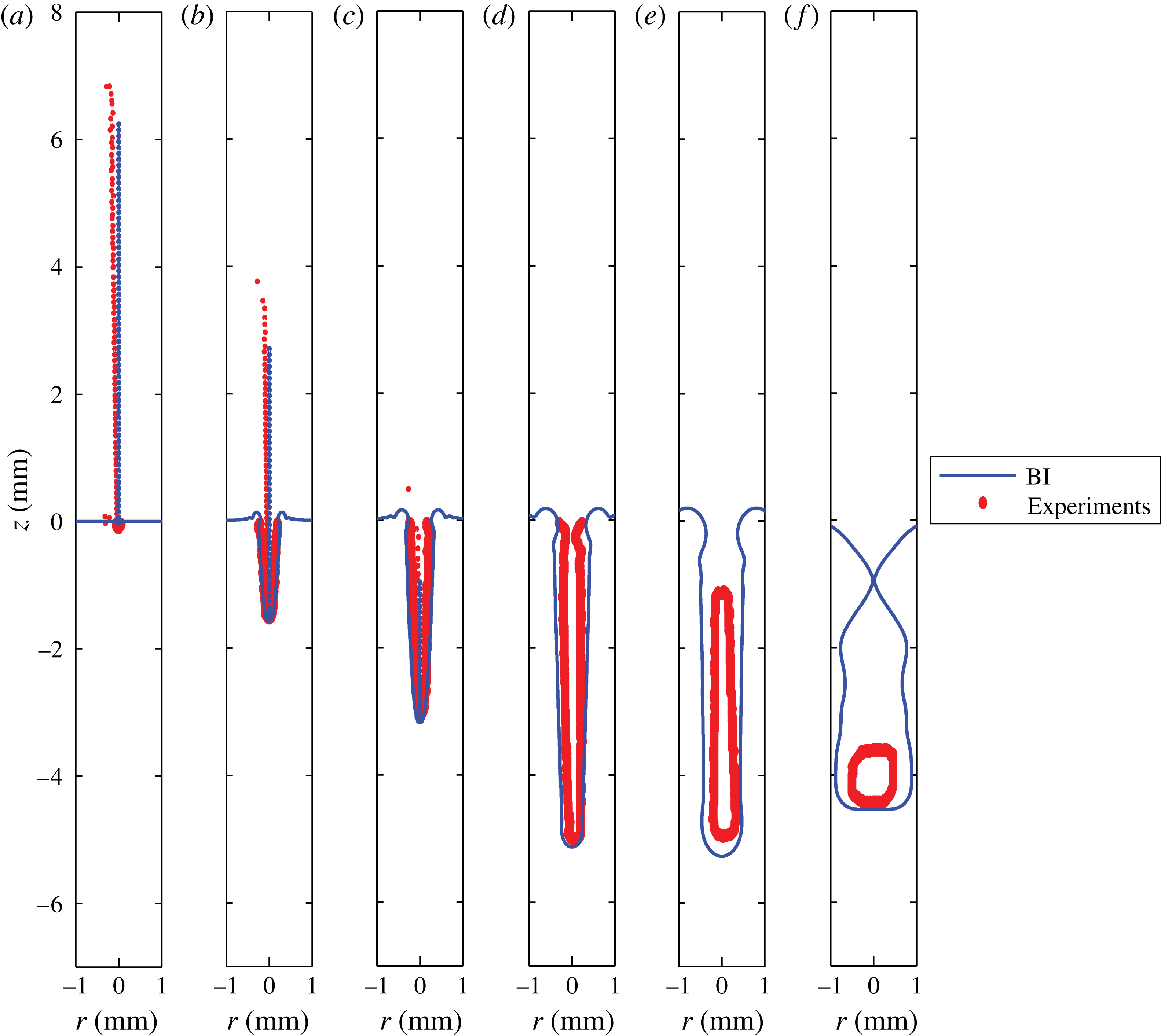
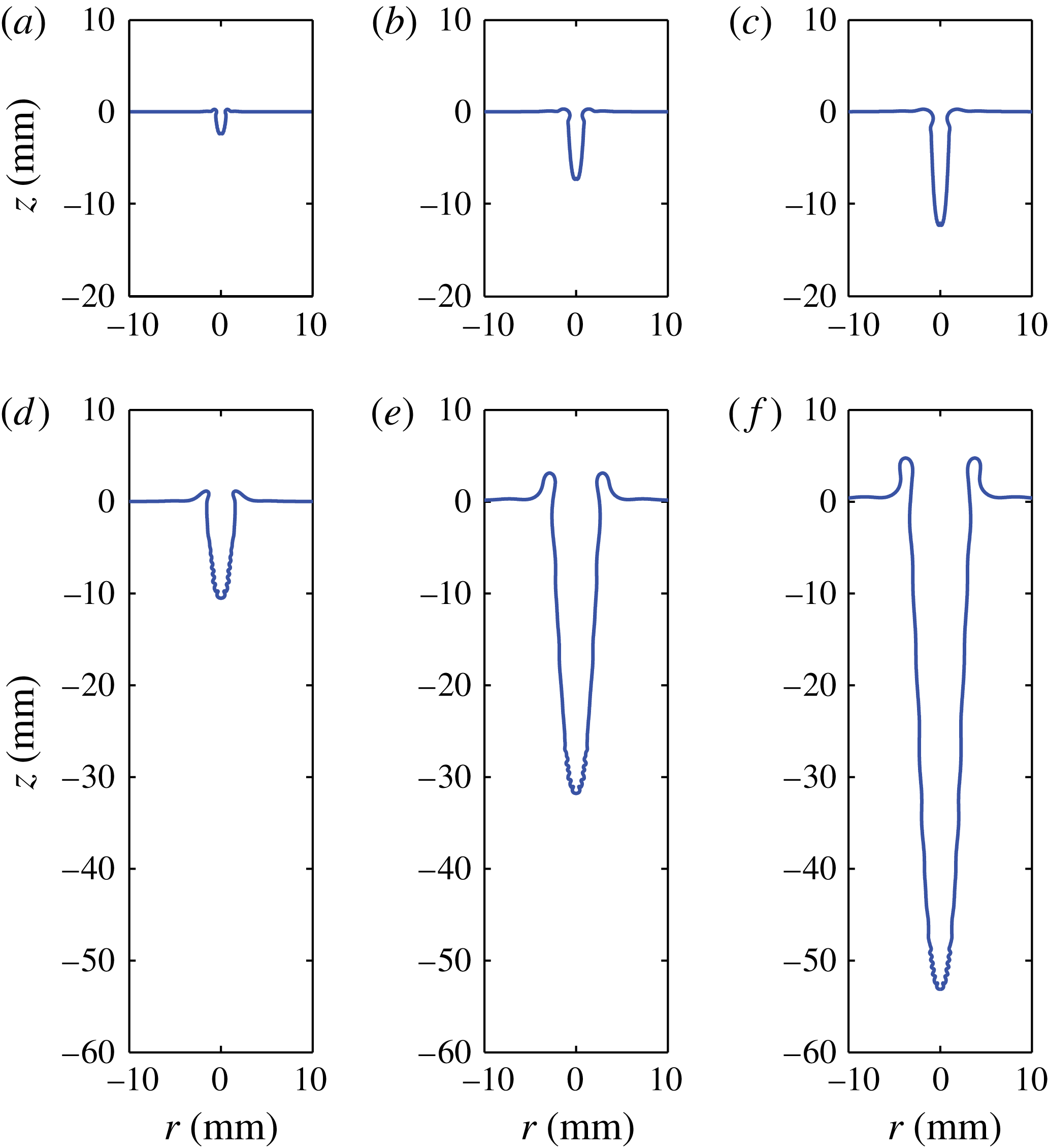
To quantitatively compare the experimental and numerical cavity contours, figure 3 shows a time sequence of snapshots during the formation and collapse of the cavity, for the parameters
 $R_{0}=20~{\rm\mu}\text{m}$
,
 $U_{0}=26.75~\text{m s}^{-1}$
and
 $f=290~\text{kHz}$
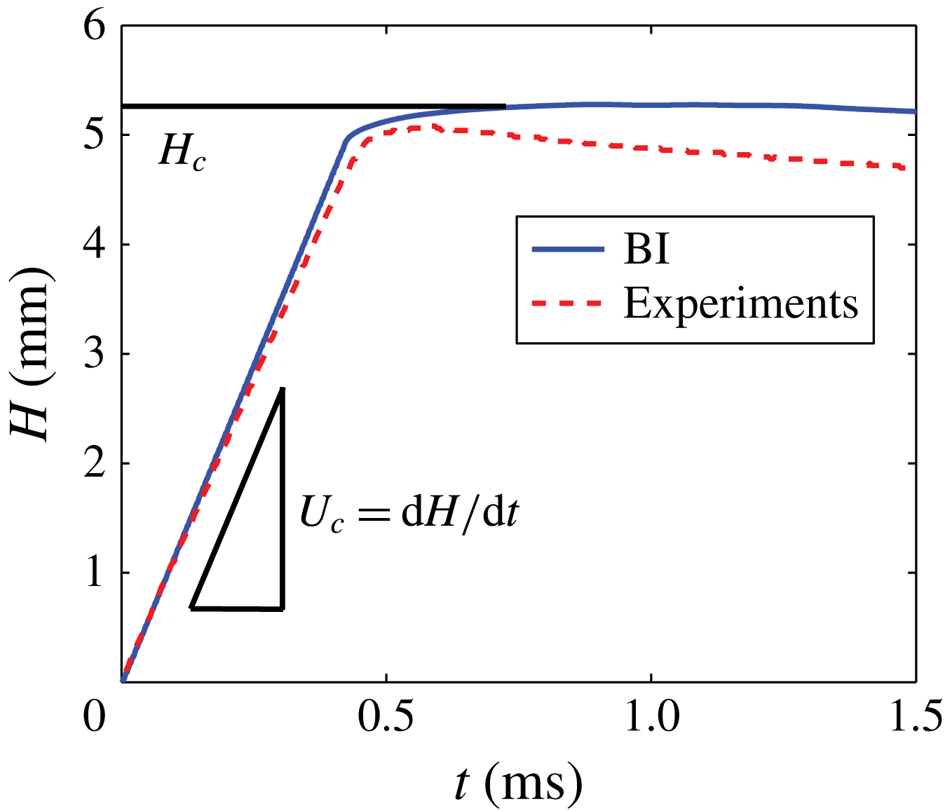
. This comparison has been applied for a finite drop train which contains about 85 drops. To do a good comparison for the deep cavities also, the influence of hydrostatics is also involved in the simulations (which only makes a difference in the latter stages, see § 2.1). The thick red lines represent the experimental results. Since we needed to visualize different length scales of the cavity (including the final cavity with its large final depth), we have to take into account an experimental uncertainty, based on pixel resolution, which is reflected in the thickness of the lines. The superimposed blue lines show the results of the BI simulation. The agreement between the experiment and the simulations is very good up to about 0.275 ms. After that, we observe substantial differences, though the downward growth speed of the cavity and the depth of the cavity at the time of its collapse continue to match very well. This is further illustrated in figure 4, where we plot the cavity height versus time.
Direct comparison between experimental and numerical (BI) results of the cavity contours, for drop radius
 $R_{0}=20~{\rm\mu}\text{m}$
, impact velocity
 $U_{0}=26.75~\text{m s}^{-1}$
and frequency
 $f=290~\text{kHz}$
: (a) 0.008 ms; (b) 0.138 ms; (c) 0.275 ms; (d) 0.508 ms; (e) 0.808 ms; (f) 2.988 ms. The downward growth speed of the cavity
 $U_{c}$
and the final depth
 $H_{m}$
match very well (also see figure 4), but there are also differences between the experiments and the simulations. The most obvious difference is that after
 $t\approx 0.275~\text{ms}$
the width of the cavity in the experiments is smaller than the cavity width resulting from simulations and, related to this, the collapse of the cavity occurs much faster in the experiments than in the numerical simulations. We attribute this to the influence of the streaming air.

Direct comparison between experimental and numerical (BI) results of the cavity depth versus time, for drop radius
 $R_{0}=20~{\rm\mu}\text{m}$
, impact velocity
 $U_{0}=26.75~\text{m s}^{-1}$
and frequency
 $f=290~\text{kHz}$
(also see figure 3). The downward growth speed of the cavity
 $U_{c}$
and the depth at the instant of the collapse,
 $H(t=0.5~\text{ms})$
match very well.

However, there are also significant differences between the experimental and numerical results. First of all, the red dots in figure 3 reveal that the drop train in the experiments was not as uniformly aligned as implemented in the numerical simulations. In particular, in the beginning (lowest part) of the train, drops were bunched up and were slowed down with respect to the ‘average’ velocity of the train, whereas at the top of the train, the spacing in between the drops was found to be increased. These effects are caused by the drag induced by the air which surrounds the falling drops. This is why the last part of the train in experiments does not have a significant influence on the formed cavity, and we account for this by a decreased number of drops in the simulated drop train (70 instead of
 ${\sim}85$
). For the same reason, we are only able to fairly compare experiments and simulations for rather long drop trains, such that the mentioned effects are the least pronounced.
Second, it can be observed that the width of the cavity in the experiments is significantly smaller than the cavity width in the simulations, particularly at later times. This effect also leads to an earlier collapse of the cavity in the experiments compared with the simulations, and the slow decrease of
 $H$
over time after the end of the drop train (
 $t\approx 0.5~\text{ms}$
) for the experimental result shown in figure 4. We mainly attribute these effects to the influence of the streaming air within the cavity. Here it is good to note that for the case of a disk plunging onto a pool, where the influence of air was included in the BI simulations, the effect of the airflow was only visible for the very final stages of the cavity collapse (Gekle et al.
Reference Gekle, van der Bos, Bergmann, van der Meer and Lohse2008, Reference Gekle, Snoeijer, Lohse and van der Meer2009, Reference Gekle, Peters, Gordillo, van der Meer and Lohse2010). It is however plausible that the small length scale of our problem, together with the presence of the high-speed falling drops within the cavity, significantly increase the influence of the air. Namely, if we assume that the air flows with the speed of the falling drops,
 $26.75~\text{m s}^{-1}$
, this results in a Reynolds number of the gas
 $\mathit{Re}_{g}={\it\rho}_{g}R_{0}U_{0}/{\it\eta}_{g}$
of order 10–100. Here,
 ${\it\rho}_{g}$
and
 ${\it\eta}_{g}$
are the density and viscosity of air, respectively,
 $1.204~\text{kg m}^{-3}$
, and
 $1.82\times 10^{-5}~\text{Pa s}$
. Thus, neglecting the effects of the air viscosity, the dynamic pressure drop with respect to the pressure at the cavity walls is of the order of
 ${\it\rho}_{g}U_{0}^{2}\sim 1000~\text{Pa}$
. This pressure drop sucks in the liquid with
 ${\it\rho}_{g}U_{0}^{2}\sim {\it\rho}U_{l}^{2}$
, where
 $U_{l}$
is the induced inward speed of the liquid cavity walls, which gives an estimation for the liquid velocity of order
 $1~\text{m s}^{-1}$
. Since the process of cavity formation takes
 ${\sim}1~\text{ms}$
, the deviation of the cavity shape is expected to be of the order of
 $1~\text{mm}$
, which is indeed consistent with the difference between experiment and simulation. Also consistent with this reasoning is that the width of the experimental cavity and that resulting from the simulations deviate the most at the top of the cavity, where the suction of the flowing air has had its influence for the largest time interval. Note, once again, that this deviation is particularly visible in the latter stages, after
 $t\approx 0.275~\text{ms}$
. In the beginning of the cavity development, experiment and simulation agree. Also the maximum width of the cavity is predicted correctly by the simulations, as will be shown more explicitly later on in this paper.
3.2 Cavity shape
The robustness of the slender shape of the cavity is evidenced by figure 5, which contains two more time sequences resulting from the BI simulations, now for two different Weber numbers. Here we used
 $R_{0}=100~{\rm\mu}\text{m}$
,
 $U_{0}=8.5~\text{m s}^{-1}$
and
 $85.4~\text{m s}^{-1}$
and
 $f=30~\text{kHz}$
, corresponding to
 $\mathit{We}=100$
and 10 000, and
 $\widetilde{f}=0.70$
and 0.07, respectively.
Time sequences from BI simulations for two different Weber numbers: (a–c)
 $\mathit{We}={\it\rho}R_{0}U_{0}^{2}/{\it\gamma}=100$
,
 $\widetilde{f}=0.7$
(for
 $U_{0}=8.5~\text{m s}^{-1}$
); and (d–f)
 $\mathit{We}=10\,000$
,
 $\widetilde{f}=0.07$
(for
 $U_{0}=85~\text{m s}^{-1}$
) (in both cases
 $R_{0}=100~{\rm\mu}\text{m}$
and
 $f=30~\text{kHz}$
). The profiles are shown at times
 $t=0.6$
, 1.8 and 3 ms. Obviously, the higher-velocity drops create a cavity with larger depth and width.

Cavity shapes for three different Weber numbers
 $\mathit{We}={\it\rho}R_{0}U_{0}^{2}/{\it\gamma}$
(a), and at three different times after the first impact at
 $t=0$
(b), shown on doubly logarithmic scale: (a)
 $U_{0}=8.5~\text{m s}^{-1}$
,
 $27.0~\text{m s}^{-1}$
, and
 $85.4~\text{m s}^{-1}$
at
 $t=6.1~\text{ms}$
(
 $tU_{0}/R_{0}=520$
), 3.2 ms (
 $tU_{0}/R_{0}=870$
) and 3.0 ms (
 $tU_{0}/R_{0}=2560$
), respectively; (b)
 $\mathit{We}=10\,000$
at three different times. For both panels
 $R_{0}=100~{\rm\mu}\text{m}$
and
 $f=30~\text{kHz}$
. We find that for large Weber number and long times after the first impact, the cavity shape approaches a parabola, i.e.
 $(z(r)+H)\sim r^{2}$
. For smaller Weber numbers this asymptotic stage is not reached, because surface tension makes the collapse behaviour at the top of the cavity too dominant.

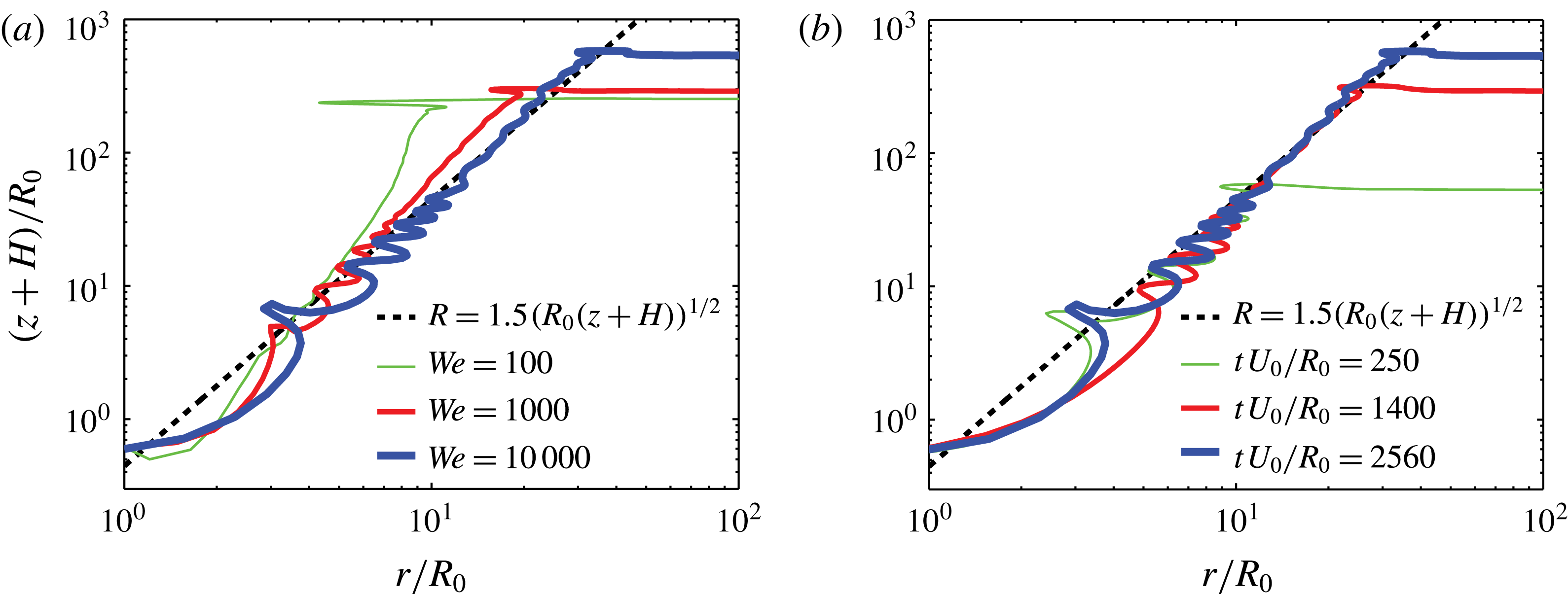
Figure 6(a) is a doubly logarithmic plot of the resulting cavity shapes for three different simulations with
 $\mathit{We}=100$
, 1000 and 10 000 (including those of figure 5). Figure 6(a) shows that for large enough Weber number, the cavity profile is parabolic:
 $R\sim (z+H)^{1/2}$
, where we corrected for the instantaneous depth of the cavity and
 $(z+H)$
is the vertical coordinate measured from the bottom at
 $z=-H(t)$
. This parabolic similarity profile is valid between the lower part of the cavity, where there are traveling surface waves resulting from the separate drop-pool collisions, and the top part of the cavity, where the surface tension driven collapse takes place (as we will discuss in § 3.3). The larger the Weber number, the more clearly the parabolic shape can be recognized: for the smallest Weber number plotted, the asymptotic stage is not reached, because surface tension makes the collapse behaviour at the top of the cavity too dominant. Figure 6(b) shows the profiles for
 $\mathit{We}=10\,000$
at three different times. Together, the panels of figure 6 show that the parabolic profile can be observed for large enough Weber number and at sufficiently long time after the first impact.
We can understand the parabolic shape of the cavity as follows. Since the cavity has a slender geometry, the fluid flow is predominantly oriented in horizontal slices. Hence, we can apply the two-dimensional Rayleigh equation in cylindrical coordinates. Neglecting the influence of hydrostatics, one obtains (Prosperetti Reference Prosperetti1977; Lohse et al. Reference Lohse, Bergmann, Mikkelsen, Zeilstra, van der Meer, Versluis, van der Weele, van der Hoef and Kuipers2004; Bergmann et al. Reference Bergmann, van der Meer, Stijnman, Sandtke, Prosperetti and Lohse2006)
 $$\begin{eqnarray}\left(R\frac{\text{d}^{2}R}{\text{d}t^{2}}+\left(\frac{\text{d}R}{\text{d}t}\right)^{2}\right)\log \left(\frac{R}{R_{\infty }}\right)+\frac{1}{2}\left(\frac{\text{d}R}{\text{d}t}\right)^{2}=-\frac{{\it\gamma}{\it\kappa}}{{\it\rho}}\approx \frac{{\it\gamma}}{{\it\rho}R},\end{eqnarray}$$
where
 $R_{\infty }$
is an external length scale of the problem that has a weak (logarithmic) influence on the analysis below (Lohse et al.
Reference Lohse, Bergmann, Mikkelsen, Zeilstra, van der Meer, Versluis, van der Weele, van der Hoef and Kuipers2004; Bergmann et al.
Reference Bergmann, van der Meer, Stijnman, Sandtke, Prosperetti and Lohse2006; Eggers et al.
Reference Eggers, Fontelos, Leppinen and Snoeijer2007; Gekle et al.
Reference Gekle, Snoeijer, Lohse and van der Meer2009). In the last approximation we neglected the axial contribution to the curvature; the axial curvature is much smaller than the radial curvature due to the slenderness of the cavity. At large
 $\mathit{We}$
, we may neglect the right-hand side during the first instances of the cavity formation, i.e. at small distance
 $z+H$
. Hence, since
 $R_{\infty }\gg R$
, the dynamics are determined by
 $R(\text{d}^{2}R/\text{d}t^{2})+(\text{d}R/\text{d}t)^{2}\approx 0$
, which has the solution
 $R(t)\sim (t-t_{0})^{1/2}$
, where
 $t=H/U_{c}$
is the time after the first impact on the initially flat pool (
 $t=0$
) at which the cavity reaches depth
 $H$
,
 $t_{0}=-z/U_{c}$
(recall that
 $z$
is negative below the pool surface) and
 $U_{c}=\text{d}H/\text{d}t$
is the (constant) downward growth speed of the cavity. This implies
 $$\begin{eqnarray}R(z,t)\sim \sqrt{R_{0}(z+H)}=\sqrt{R_{0}(z+U_{c}t)}.\end{eqnarray}$$
This is the similarity profile, to which the curves of figure 6 converge, for large Weber number, sufficiently long after the first impact, and away from the bottom and top of the cavity. The dashed line represents the prediction (3.2), with a fitted prefactor of 1.5.
3.3 Cavity dynamics
Two important questions arise from the preceding analysis: what is the downward expansion speed of the cavity
 $U_{c}$
as a function of the impact parameters, and when does surface tension start to act against the expansion of the cavity?
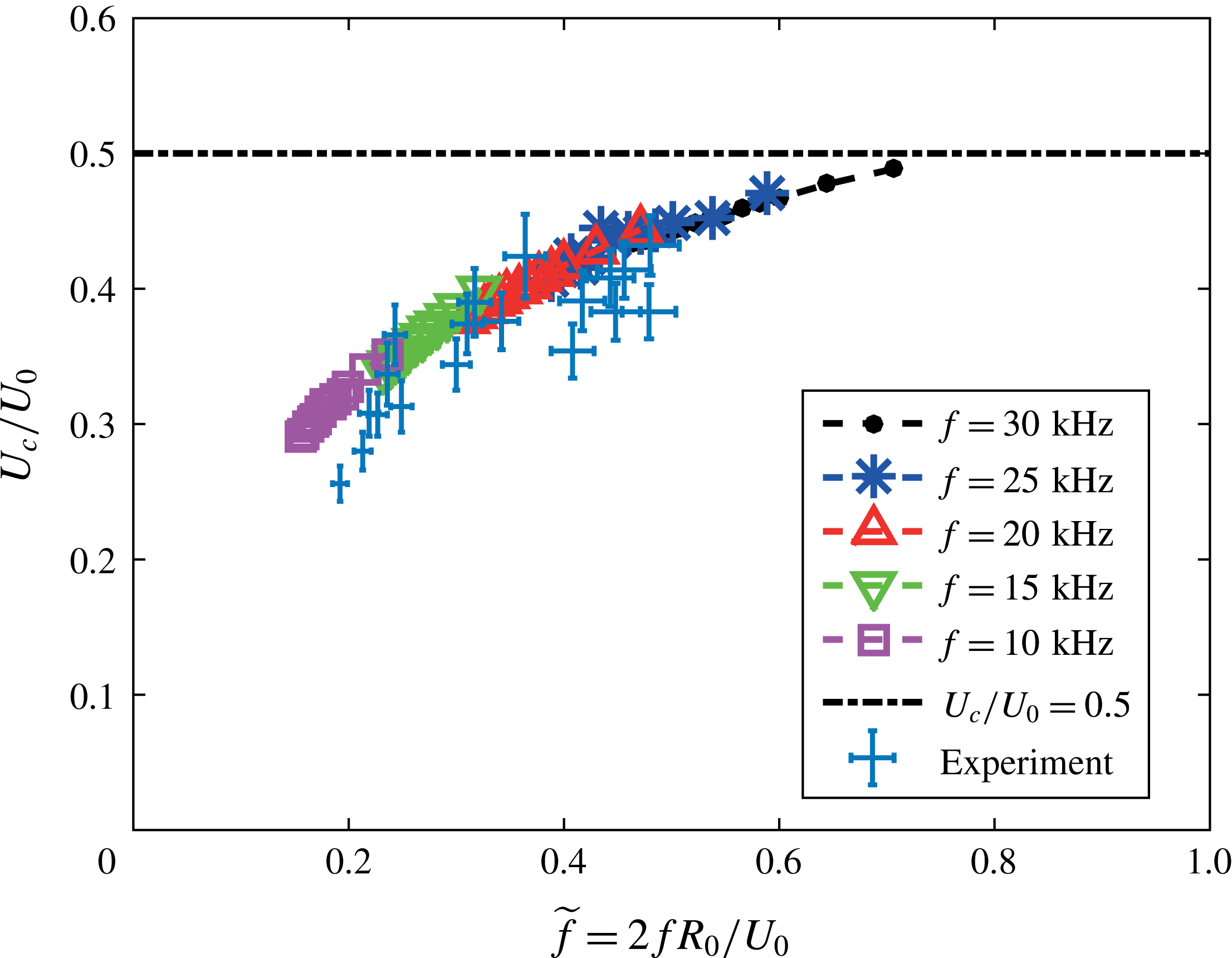
Figure 7 shows
 $U_{c}/U_{0}$
as a function of the ratio
 $\widetilde{f}=2fR_{0}/U_{0}$
. We superimposed experimental results for varying
 $\widetilde{f}$
and
 $\mathit{We}$
(by varying the drop frequency in the experiments, also the drop sizes and velocities are modified), which shows reasonable agreement with the numerical results. The large error estimates are particularly due to the limited pixel resolution, as explained in § 3.1. The five different numerical datasets show the results for five drop frequencies
 $f=10{-}30~\text{kHz}$
, for varying impact velocities
 $U_{0}=7{-}13~\text{m s}^{-1}$
. Thus, the Weber number strongly varies over the data points shown in the figure; every data point belongs to a different set of (
 $\mathit{We}$
,
 $\widetilde{f}$
), which is why we choose to mention the dimensional frequency in the legend, while we show dimensionless plots. As explained in § 2.2.2, close to the limit
 $\widetilde{f}\rightarrow 1$
, the number of reconnections per time unit, and thus the relative importance of the corresponding numerical artifacts, is large, which is why we do not show our results for
 $\widetilde{f}>0.7$
. Interestingly,
 $U_{c}/U_{0}$
converges to
 $1/2$
for
 $\widetilde{f}\rightarrow 1$
. Here
 $\widetilde{f}=1$
would be the situation of a drop train with zero spacing, which corresponds to the special case in which momentum is continuously applied to the pool/cavity bottom. This is reminiscent of the continuously impacting jet onto a pool, as described in Oguz et al. (Reference Oguz, Prosperetti and Kolaini1995). One of the results for the continuously impacting jet scenario described in this work is that the downward expansion speed of the cavity is exactly one half of the impact speed of the jet,
 $U_{c}/U_{0}=1/2$
. This ratio
 $1/2$
is indeed approached in our simulations. At smaller frequencies, the net momentum transfer per time unit decreases, and the downward expansion speed of the cavity will thus be smaller, giving a qualitative explanation of our findings in figure 7.
The downward cavity growth velocity
 $U_{c}$
divided by the drop impact speed
 $U_{0}$
plotted against the ratio
 $\widetilde{f}=2fR_{0}/U_{0}$
for several values of the Weber number
 $\mathit{We}$
and the drop frequency
 $f$
. Simulation results for
 $R_{0}=100~{\rm\mu}\text{m}$
. As long as
 $f\gg 1/t_{s}$
, with
 $t_{s}=\sqrt{{\it\rho}R_{0}^{3}/{\it\gamma}}$
the typical capillary oscillation time scale of the drops, we find that
 $U_{c}/U_{0}$
universally depends on
 $\widetilde{f}$
, i.e.
 $U_{c}/U_{0}$
is independent of
 $\mathit{We}$
, and converges to
 $1/2$
for
 $\widetilde{f}\rightarrow 1$
, where the droplet train turns into a continuous jet. Experimental results for varying
 $\widetilde{f}$
and
 $\mathit{We}$
are superimposed, showing reasonable agreement. The error estimate in the experiments is particularly based on the limited pixel resolution.

The Weber number strongly varies over the data in figure 7, but the relation between
 $U_{c}/U_{0}$
and
 $\widetilde{f}$
appears to be universal, in the sense that it is independent of
 $\mathit{We}$
. However, this universality will only hold if the collapse time of the small cavity created by the single drop impact is much larger than the time it takes until the next drop impacts, which is generally true for our impact parameters. Otherwise, obviously, since the surface tension influences the local cavity collapse, the relation between
 $U_{c}/U_{0}$
and
 $\widetilde{f}$
will have a Weber dependence.
With this result of
 $U_{c}$
as a function of the frequency
 $\widetilde{f}$
, we basically know all of the dynamic details of the downward translating parabolic cavity, and we are able to predict its collapse. The time at which surface tension will start to pull back the cavity walls can be predicted by solving (3.1) without neglecting the influence of the surface tension. This can be done analytically, as shown in the appendix A, but can also be appreciated from a dimensional argument that will be provided below. For this one must introduce a velocity scale, for which we choose the downward speed of the cavity
 $U_{c}$
instead of
 $U_{0}$
. This defines a ‘modified’ Weber number
 $\mathit{We}_{m}$
as
 $$\begin{eqnarray}\mathit{We}_{m}=\frac{{\it\rho}R_{0}U_{c}^{2}}{{\it\gamma}}=\mathit{We}\left(\frac{U_{c}}{U_{0}}\right)^{2},\end{eqnarray}$$
and in the remainder of this section we will plot our results as a function of
 $\mathit{We}_{m}$
.
We will show how the collapse of the cavity depends on
 $U_{c}$
and the other parameters. For this, we need to separate two cases, which are basically short and long drop trains. More specifically, we distinguish trains for which the collapse of the cavity occurs after the full drop train has impacted, as in our experimental comparison (figures 3 and 4), and trains for which the collapse of the cavity occurs before the end of the drop train impact. In the first case, the cavity depth at the moment of its collapse,
 $H_{coll}$
, is determined by the number of drops
 $N$
in the train,
 $H_{c}=H_{coll}\sim NU_{c}/f$
; in the second case, this depth is determined by the time at which the cavity walls touch the symmetry axis (or the drops). Note that in the second case,
 $H_{c}$
is in general larger than
 $H_{coll}$
; experiments show that after the cavity walls hit the symmetry axis, the drops within the entrained bubble will still continue impacting on the bubble bottom, an effect that could further increase the depth of the bubble. In that case, to predict
 $H_{c}$
, one needs to take into account the bubble deformation dynamics, which we leave for the moment. Thus, we focus on the prediction of
 $H_{coll}$
. The time at which surface tension is able to influence the cavity walls,
 $t_{coll}$
, can be predicted by comparing the dynamic pressure of the radially expanding cavity (which decreases in time, and is the smallest at the top of the cavity, where the parabola that describes it is the widest) and the Young–Laplace pressure based on the azimuthal curvature of the cavity:
 $$\begin{eqnarray}{\it\rho}\left(\frac{\text{d}R_{z=0}}{\text{d}t}\right)^{2}\sim \frac{{\it\gamma}}{R_{z=0}},\end{eqnarray}$$
where
 $R_{z=0}$
is the cavity radius at the pool surface,
 $z=0$
. Substituting the dynamic profile for the cavity found in § 3.2,
 $R_{z=0}(t)\sim \sqrt{R_{0}H(t)}=\sqrt{R_{0}U_{c}t}$
, from which
 $\text{d}R_{z=0}/\text{d}t\sim \sqrt{R_{0}U_{c}/t}$
, gives a prediction of the time at which
 $R_{z=0}$
reaches the maximum expansion radius of the cavity, which we call
 $t_{coll}$
:
 $$\begin{eqnarray}t_{coll}\sim \frac{{\it\rho}^{2}R_{0}^{3}U_{c}^{3}}{{\it\gamma}^{2}}=t_{s}\mathit{We}_{m}^{3/2},\end{eqnarray}$$
where
 $t_{s}=\sqrt{{\it\rho}R_{0}^{3}/{\it\gamma}}$
is the typical capillary time scale at which a drop with radius
 $R_{0}$
oscillates (Lamb Reference Lamb1957). When we insert
 $t_{coll}$
in the similarity profile we can calculate the maximum radius
 $R_{c}$
of the cavity:
 $$\begin{eqnarray}R_{c}\sim \sqrt{R_{0}U_{c}t_{coll}}\sim R_{0}\mathit{We}_{m}.\end{eqnarray}$$
Combining (3.5) and (3.6), we find that the typical time at which the cavity starts to collapse is the capillary time based on the maximum radius of the cavity (
 $t_{coll}\sim \sqrt{{\it\rho}R_{c}^{3}/{\it\gamma}}$
), as previously found by Aristoff & Bush (Reference Aristoff and Bush2009) for the collapse of a cavity generated by the impact of a solid sphere. The depth of the cavity at the time of its collapse,
 $H_{coll}$
can now be predicted by multiplying the expansion velocity by the collapse time:
 $$\begin{eqnarray}H_{coll}\sim U_{c}t_{coll}\sim U_{c}t_{s}\mathit{We}_{m}^{3/2}\sim R_{0}\mathit{We}_{m}^{2}.\end{eqnarray}$$
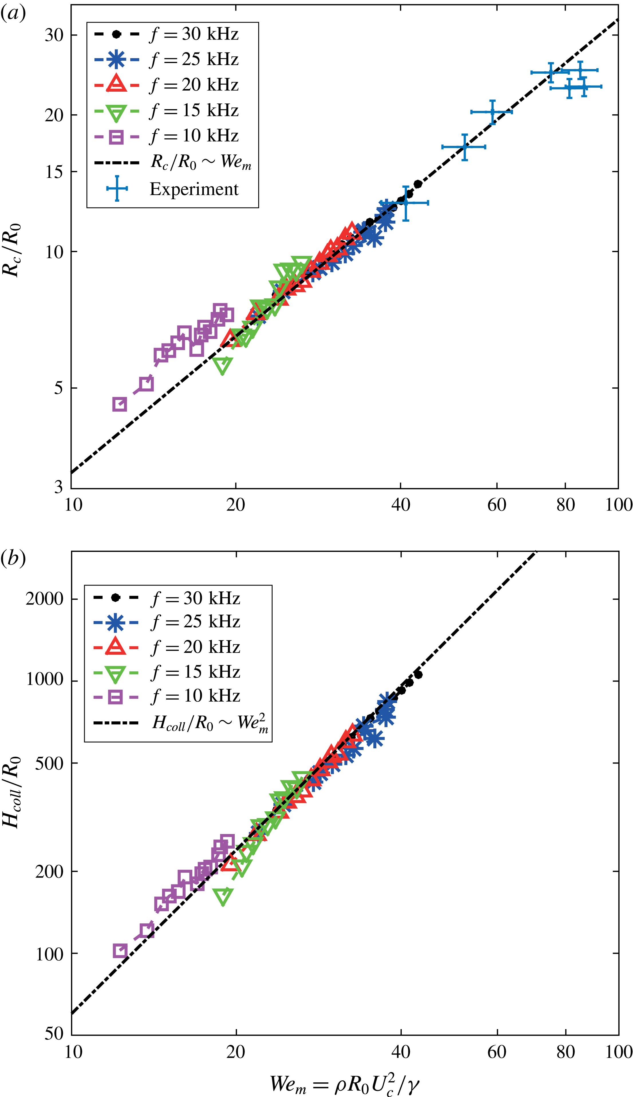
From figure 8(a,b), which show the BI simulation results of our parameter scan for
 $R_{c}$
and
 $H_{coll}$
, respectively, one can appreciate that the above scaling results agree with the BI results. The curves seem to be universal, independent of the drop frequency
 $\widetilde{f}$
, but note that the
 $f$
-dependence is taken into account by means of
 $U_{c}$
. This confirms that
 $\mathit{We}_{m}$
, and not
 $\mathit{We}$
, is the proper dimensionless parameter to analyse the maximum cavity radius and the cavity collapse. Note that
 $\mathit{We}_{m}$
naturally varies over a smaller range than
 $\mathit{We}$
, due to its definition (3.3), setting a limit on the range in figure 8.
(a) Maximum radius of the cavity
 $R_{c}$
and (b) depth of the cavity
 $H_{coll}$
at the moment of its collapse, plotted against the modified Weber number
 $\mathit{We}_{m}={\it\rho}R_{0}U_{c}^{2}/{\it\gamma}$
based on the vertical cavity growth speed
 $U_{c}$
for several
 $\mathit{We}$
and
 $f$
.
 $R_{0}=100~{\rm\mu}\text{m}$
. We find a universal behaviour with respect to
 $\mathit{We}_{m}$
, independent of
 $\widetilde{f}$
. Superimposed are the scaling predictions:
 $R_{c}/R_{0}\sim \mathit{We}_{m}$
, and
 $H_{coll}/R_{0}\sim \mathit{We}_{m}^{2}$
, with which we find very good agreement. The prefactors of the fits are 0.325 and 0.600 respectively for (a,b). The maximum reached cavity widths in the experiments are superimposed in (a), which also shows good agreement with the scaling predictions. The error estimate in the experiments is particularly based on the limited pixel resolution.

In figure 8(a) we superimposed the simulation results for the maximum cavity width for several
 $\mathit{We}_{c}$
, which also shows a good agreement with our scaling predictions. Again, all of the parameters
 $R_{0}$
,
 $U_{0}$
and
 $f$
vary for these experimental measurements, which even more confirms the universal behaviour within the shown parameter regime. Since the cavity collapses much earlier in the experiments compared with the numerical simulations (see § 3.1), we could not do such a one-to-one comparison between the experiments and numerical simulations for the final cavity depth.
4 Discussion
Summarizing, we found that the expansion of the cavity resulting from a microdrop train impact can be described as a purely inertial mechanism, except for the collapse region that is a result of the capillary forces. From solving the 2D Rayleigh equation, we concluded that the cavity shape is a parabola, which translates downward with a constant velocity
 $U_{c}$
. We showed that
 $U_{c}/U_{0}$
only depends on the aspect ratio
 $\widetilde{f}$
of the drop train, i.e. the ratio of drop diameter to drop distance in the train. In addition, we were able to predict the collapse duration
 $t_{coll}$
, and the cavity depth
 $H_{coll}$
at the moment of the collapse.
When comparing with experiments there is an important caveat, namely that we can only expect the theory (and consequently also the comparison to the simulations) to work when the influence of air is not too significant. The most important difference in the limited range of parameter space that we are able to access experimentally, is that, at later times, the width of the cavity in the experiments, is smaller than the width in the numerical simulations, due to, most likely, the influence of the streaming air, which has been neglected. Up to the time that the maximum cavity depth is reached, our predictions for the depth of the cavity are still accurate for the experiment. This originates from the fact that the dynamics at the bottom of the cavity, in particular
 $U_{c}$
, is hardly influenced by the airflow. Thus, the collapse in experiments occurs earlier than predicted, but after that collapse, the bottom of the cavity keeps expanding with the same
 $U_{c}$
, until the last drop in the drop train inside the cavity has impacted, and the instantaneous depths are predicted correctly, as shown in figure 4. Also the maximum widths are predicted correctly, as shown in figure 8(a). In the experimentally accessible range, our simulation method appears to be an efficient way to simulate drop train impact, if one focuses on the depth of the cavity, neglecting the influence of air. Moreover, since the BI code solves the Laplace equation only along the pool surface we are able to account for the many different length scales in the problem, ranging from the cavity size, through the drop dimension, to the scale of the recombination of the free surfaces of the drop and the cavity. This would pose difficulties or at least much computational effort for most other simulation methods. However, an advantage of the use of a two-phase simulation method would be the ability to solve correctly for the influence of the local airflow, in particular the airflow induced by the falling drops, which points towards possible future work on this subject.
Other possible future studies on this subject could focus on different mechanisms of the cavity collapse and bubble formation processes. In fact such a study has been described in detail in Aristoff & Bush (Reference Aristoff and Bush2009), although that work is centred on sphere impact on a pool. Our case, the impact of a collection of liquid onto a pool, gives rise to the following question for future research: how does the mass distribution and the time scale of the impact influence the cavity shape, and thus the collapse? We already found that the impact of a jet is from a qualitative point of view not different from the impact of a drop train, except that the frequency is an explicit parameter for the latter case. We found that, in addition to the total amount of volume which impacts onto the pool, the lengthscale and timescale of the total impact is highly determinative for the cavity behaviour, because it determines the relevance of hydrostatics versus surface tension. This is an aspect of the multidroplet train problem that can not be ignored.
Acknowledgements
This work was supported by STW and NWO through a VIDI grant no. 11304. The financial support by the Austrian Federal Ministry of Economy, Family and Youth and the Austrian National Foundation for Research, Technology and Development is gratefully acknowledged as is the support from Lam Research AG.
Appendix A. Solution of the cylindrical Rayleigh equation including the influence of surface tension
Here, we analytically solve (3.1), including the Young–Laplace pressure based on the azimuthal curvature of the cavity (Kedrinskii Reference Kedrinskii2005). We start from (3.1), which we non-dimensionalize using the drop radius
 $R_{0}$
and
 $R_{0}/U_{c}$
, the drop radius over the downward cavity speed, as typical length and time scales. This gives
 $$\begin{eqnarray}\left(\frac{\text{d}}{\text{d}\widetilde{t}}\left(\widetilde{R}\frac{\text{d}\widetilde{R}}{\text{d}\widetilde{t}}\right)\right)\log \left(\frac{\widetilde{R}}{\widetilde{R}_{\infty }}\right)+\frac{1}{2}\left(\frac{\text{d}\widetilde{R}}{\text{d}\widetilde{t}}\right)^{2}=\frac{1}{\mathit{We}_{m}}\frac{1}{\widetilde{R}},\end{eqnarray}$$
where
 $\widetilde{R}=R/R_{0}$
,
 $\widetilde{R}_{\infty }=R_{\infty }/R_{0}$
,
 $\widetilde{t}=tU_{c}/R_{0}$
and
 $\mathit{We}_{m}={\it\rho}R_{0}U_{c}^{2}/{\it\gamma}$
. In the remainder of this appendix we will drop the tildes.
Writing
 $U=\text{d}R/\text{d}t$
we first note that
 $$\begin{eqnarray}\frac{\text{d}}{\text{d}t}(RU)=U^{2}+R\frac{\text{d}U}{\text{d}t}=U^{2}+\frac{1}{2}R\frac{\text{d}}{\text{d}R}(U^{2}),\end{eqnarray}$$
where we used that
 $\text{d}U/\text{d}t=\text{d}U/\text{d}R\,\text{d}R/\text{d}t=U\,\text{d}U/\text{d}R$
. With this, equation (A 1) becomes
 $$\begin{eqnarray}U^{2}\log \left(\frac{R}{R_{\infty }}\right)+\frac{1}{2}R\frac{\text{d}}{\text{d}R}(U^{2})\log \left(\frac{R}{R_{\infty }}\right)+\frac{1}{2}U^{2}=\frac{1}{\mathit{We}_{m}}\frac{1}{R}.\end{eqnarray}$$
Now let
 $x=R/R_{\infty }$
and
 $y=(\text{d}R/\text{d}t)^{2}$
. Then the above equation reads
 $$\begin{eqnarray}\frac{1}{2}x\log (x)\frac{\text{d}y}{\text{d}x}+\left(\log (x)+\frac{1}{2}\right)y=\frac{1}{\mathit{We}_{m}}\frac{1}{R_{\infty }x}.\end{eqnarray}$$
This is an ordinary linear differential equation of which the solution consists of a homogeneous part and a particular part. The homogeneous solution of
 $(1/2)x\log (x)\,\text{d}y/\text{d}x+(\log (x)+1/2)y=0$
is
 $y_{H}(x)=K/(x^{2}\log (x))$
, where
 $K$
is an integration constant. A particular solution of the shape
 $y_{P}(x)=Cx^{a}/\log (x)$
gives a solution for
 $a=-1$
and
 $C=2/(\mathit{We}_{m}R_{\infty })$
, so the full solution to (A 4) is
 $$\begin{eqnarray}y(x)=\frac{K}{x^{2}\log (x)}+\frac{2}{\mathit{We}_{m}R_{\infty }x\log (x)}.\end{eqnarray}$$
Going back to the original variables we have
 $$\begin{eqnarray}\left(\frac{\text{d}R}{\text{d}t}\right)^{2}=\left(2+\frac{K^{\prime }}{R}\right)\frac{1}{\mathit{We}_{m}R\log \left({\displaystyle \frac{R}{R_{\infty }}}\right)},\end{eqnarray}$$
with
 $K^{\prime }=KR_{\infty }^{2}\mathit{We}_{m}$
. If we scale back to the dimensional variables and substitute the initial conditions
 $R(t=0)=AR_{0}$
and
 $\text{d}R/\text{d}t(t=0)=BU_{c}$
(with
 $A$
and
 $B$
positive real numbers), the solution reads
 $$\begin{eqnarray}\left(\frac{\text{d}R}{\text{d}t}\right)^{2}=\frac{R_{0}U_{c}^{2}}{R\log \left({\displaystyle \frac{R}{R_{\infty }}}\right)}\left[\frac{2}{\mathit{We}_{m}}+{\displaystyle \frac{B^{2}A^{2}R_{0}\log \left({\displaystyle \frac{R_{0}}{R_{\infty }}}\right)-{\displaystyle \frac{2AR_{0}}{\mathit{We}_{m}}}}{R}}\right].\end{eqnarray}$$
For
 $\mathit{We}_{m}\rightarrow \infty$
, this implies
 $$\begin{eqnarray}\frac{R{\displaystyle \frac{\text{d}R}{\text{d}t}}}{R_{0}U_{c}}=AB\sqrt{\frac{\log \left({\displaystyle \frac{AR_{0}}{R_{\infty }}}\right)}{\log \left({\displaystyle \frac{R}{R_{\infty }}}\right)}},\end{eqnarray}$$
which is real and positive as long as
 $R$
and
 $R_{0}$
are smaller than
 $R_{\infty }$
.
Finally, to find the maximum expansion radius of the cavity,
 $R_{c}$
, one uses
 $\text{d}R/\text{d}t=0$
in (A 7), which leads to
 $$\begin{eqnarray}R_{c}=R_{0}\left(A+\frac{A^{2}B^{2}\mathit{We}_{m}\log \left({\displaystyle \frac{R_{\infty }}{R_{0}}}\right)}{2}\right).\end{eqnarray}$$
For large
 $\mathit{We}_{m}$
, we thus expect
 $R_{c}\sim R_{0}\mathit{We}_{m}$
, which agrees with the scaling law found on dimensional grounds (3.6).