I. INTRODUCTION
The FE simulation has become an efficient tool for predicting the geometry and mechanical properties of the final parts in industry. Reference Hopperstad, Berstad, Ilstad, Lademo and Langseth1 Hill’48 yield function considering the anisotropy of material has been widely used to simulate the forming process of sheet and tubes. Generally, the parameters of Hill’48 yield function are solved directly from the uniaxial tensile tests at 0°, 45°, and 90° with respect to the rolling direction. But for the small-sized tubes, only the uniaxial tensile test at the rolling direction can be conducted because the specimens at 45° and 90° with respect to the rolling direction can not be cut from the small-sized tubes. So only the normal anisotropy is considered in FE simulation of small-sized tube forming processes, such as bending process, Reference Zhan, Huang and Yang2 which makes the prediction accuracy of cross section dimension of small-sized tube with obvious anisotropy. Thus to obtain the material behaviors of small-sized tube in bending process, some efforts are required to determine the parameters of Hill’48 yield function.
In past decades, the inverse method has been widely used to determine the parameters of yield functions. Cooreman et al. Reference Cooreman, Lecompte, Sol, Vantomme and Debruyne3 used the inverse identification scheme to determine the parameters of Hill’48 yield function using a biaxial tensile test for describing the yield locus of DC06 steel plate. By using uniaxial tensile test and equi-biaxial tensile test, Güner et al. Reference Güner, Soyarslan, Brosius and Tekkaya4 adopted the inverse identification framework to identify the planar anisotropic parameters of the Yld2000-2D yield function for simulating the material behaviors of AA6016-T4 sheet metal. Tardif and Kyriakides Reference Tardif and Kyriakides5 proposed a systematic inverse methodology to calibrate the 18-parameter nonquadratic Yld2004-3D yield function to represent the anisotropy of Al-6061-T6 sheet metal by using uniaxial and biaxial tensile tests. In these studies, as the specimens with various dimensions can be cut directly from sheet metals, the parameters of yield function were determined according to standard tests. But the applicability of the determined parameters of yield function according to the standard tests in the real forming process was not evaluated. Cooreman et al. Reference Cooreman, Lecompte, Sol, Vantomme and Debruyne6 found that the deformation fields generated in these standard tests do not represent that generated in real forming process, so the deformation behaviors of metals in real forming process can not described exactly by the determined yield function based on standard tests. To overcome the problem, some researchers have adopted the real forming process Reference Ghouati and Gelin7 in the inverse method to identify the parameters of yield function in last few years. Chamekh et al. Reference Chamekh, Salah and Hambli8 adopted the inverse method to identify the parameters of Hill’48 yield function based on the deep drawing of a cylindrical cup. Malakizadi et al. Reference Malakizadi, Cedergren, Sadik and Nyborg9 also used the inverse method to determine the parameters of Johnson–Cook material model based on the metal cutting process. By using the inverse method combining the real forming process, the deformation behaviors of metals can be predicted more accurately by the determined parameters of yield function. For small-sized tubes, most of the standard tests can not be conducted due to the dimension restriction, so adopting the inverse method combining the real forming process to determine the parameters of yield function can be a good choice. Thus to identify the material behaviors of small-sized tubes in bending process, an inverse method combining the three-point bending is introduced to determine the parameters of Hill’48 yield function. For most of the inverse methods, the FE simulations using the updated parameters set were performed iteratively until the gap between experimentally measured results and simulation results was minimized in the optimization process. Reference Huber and Tyulyukovskiyand10 But the computational cost of iterative FE simulations is quite greedy from a CPU time point of view. To improve the efficiency of identifying the parameters of yield function, an inverse method combining the response surface methodology (RSM) was proposed. Reference Malakizadi, Cedergren, Sadik and Nyborg9,Reference Malakizadi, Sadik and Nyborg11 The FE simulations can be conducted simultaneously by using RSM, which avoids the iterative FE simulations, so the computing time was reduced highly.
In this study, the small-sized H96 brass extrusion DRRT with obvious anisotropy was selected as the study object. To obtain the material behaviors of small-sized DRRT in bending process, an inverse method combining RSM and three-point bending was proposed to determine the parameters of Hill’48 yield function. With the purpose of evaluate the reliability of the proposed inverse method, the FE simulation of three-point bending of DRRT by using three yield functions, Hill’48 yield function with the determined parameters, Hill’48 yield function only considering the normal anisotropy and Mises yield function, were conducted and the simulation results were compared with the experiment results. To evaluate the applicability of the proposed inverse method in real forming process, the FE simulations of rotary draw bending of DRRT based on the three yield functions were also conducted and the simulation results were compared with the experimental ones.
II. THE INVERSE PARAMETERS IDENTIFICATION OF HILL’48 YIELD FUNCTION COMBINING RSM AND THREE-POINT BENDING
A. Hill’48 yield function
The H96 brass DRRT is used as the study object. In bending process, DRRT is usually considered to be in a plane stress state. And then Hill’48 yield function becomes:
 $$F\left( \sigma \right) = \left( {G + H} \right)\sigma _{xx}^2 - 2H{\sigma _{xx}}{\sigma _{yy}} + \left( {H + F} \right)\sigma _{yy}^2 + 2N\sigma _{xy}^2 = {\bar \sigma ^2}\quad ,$$
where σ xx and σ yy are the normal stress in the rolling direction and the direction transversal to the rolling direction. σ xy is the shear stress. F, G, H, and N are the material parameters deciding the anisotropic plasticity potential of Hill’48 yield function. These parameters are usually determined based on the Lankford’s coefficient (r-value) obtained by uniaxial tensile tests according to Eq. (2). Reference Hill12
 $$F = {{{r_0}} \over {\left( {1 + {r_0}} \right){r_{90}}}};\;G = {1 \over {1 + {r_0}}};\;H = {{{r_0}} \over {1 + {r_0}}};\;N = {{\left( {1 + 2{r_{45}}} \right)\left( {{r_0} + {r_{90}}} \right)} \over {2\left( {1 + {r_0}} \right){r_{90}}}}\quad ,$$
where r 0, r 45, and r 90 are the r-values at 0°, 45°, and 90° with respect to rolling direction in uniaxial tensile test, respectively.
But when Hill’48 yield function is used in commercial software, ABAQUS, the anisotropic plasticity potential of Hill’48 yield function is determined by the user input parameters R 11, R 22, R 33, and R 12. The relationship between the material parameters of Hill’48 yield function and user input parameters are shown in Eq. (3) Reference Hill12 :
 $$\left\{ {\matrix{ {F = {1 \over 2}\left( {{1 \over {R_{22}^2}} + {1 \over {R_{33}^2}} - {1 \over {R_{11}^2}}} \right)} \cr {G = {1 \over 2}\left( {{1 \over {R_{33}^2}} + {1 \over {R_{11}^2}} - {1 \over {R_{22}^2}}} \right)} \cr \matrix{ H = {1 \over 2}\left( {{1 \over {R_{11}^2}} + {1 \over {R_{22}^2}} - {1 \over {R_{33}^2}}} \right) \hfill \cr N = {3 \over {2R_{12}^2}} \hfill \cr} \cr} } \right.\quad .$$
The used input parameters R 11, R 22, R 33, and R 12 are defined with respect to a user-defined reference yield stress, σ0. It has been known that R 11 = σs11/σ0. σs11 is the measured yield stress in rolling direction. Generally, the reference yield stress σ0 is defined to be equal to σs11, so R 11 is equal to 1. And then R 22, R 33, and R 12 are the parameters needed to be determined for Hill’48 yield function. Based on Eqs. (2) and (3), the relationship between Lankford’s coefficient, r 0, r 45, and r 90, and the used input parameters R 22, R 33, and R 12 can be obtained according to Eq. (4) Reference Yan, Wang and Li13 :
 $$\left\{ {\matrix{ {{R_{22}} = \sqrt {{{1 + \left( {{1 \mathord{\left/ {\vphantom {1 {{r_0}}}} \right. \kern-\nulldelimiterspace} {{r_0}}}} \right)} \over {1 + \left( {{1 \mathord{\left/ {\vphantom {1 {{r_{90}}}}} \right. \kern-\nulldelimiterspace} {{r_{90}}}}} \right)}}} } \cr {{R_{33}} = \sqrt {{{1 + \left( {{1 \mathord{\left/ {\vphantom {1 {{r_0}}}} \right. \kern-\nulldelimiterspace} {{r_0}}}} \right)} \over {\left( {{1 \mathord{\left/ {\vphantom {1 {{r_0}}}} \right. \kern-\nulldelimiterspace} {{r_0}}}} \right) + \left( {{1 \mathord{\left/ {\vphantom {1 {{r_{90}}}}} \right. \kern-\nulldelimiterspace} {{r_{90}}}}} \right)}}} } \cr {{R_{12}} = \sqrt {{{3\left[ {1 + \left( {{1 \mathord{\left/ {\vphantom {1 {{r_0}}}} \right. \kern-\nulldelimiterspace} {{r_0}}}} \right)} \right]} \over {\left[ {\left( {{1 \mathord{\left/ {\vphantom {1 {{r_0}}}} \right. \kern-\nulldelimiterspace} {{r_0}}}} \right) + \left( {{1 \mathord{\left/ {\vphantom {1 {{r_{90}}}}} \right. \kern-\nulldelimiterspace} {{r_{90}}}}} \right)} \right]\left[ {1 + 2{r_{45}}} \right]}}} } \cr} } \right.\quad .$$
According to Eq. (4), the parameters of Hill’48 yield function, R 22, R 33, and R 12, can be determined by using the r-values at 0°, 45°, and 90° with respect to rolling direction in uniaxial tensile test. But the uniaxial tensile tests at 45° and 90° with respect to rolling direction can not be conducted for DRRT, so an inverse method combining RSM and three-point bending is introduced to identify the parameters, R 22, R 33, and R 12.
B. The three-point bending of DRRT
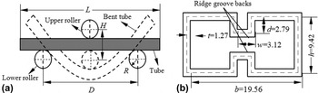
Figure 1(a) shows the sketch of three-point bending of DRRT. Two lower rollers are fixed in a horizontal line with a span D = 65 mm and an upper roller is located above the middle of two lower rollers. The radius R of roller is 10 mm. The DRRT is placed between the upper and lower rollers. The cross sectional shape of DRRT used in the study is shown in Fig. 1(b). The length L of DRRT is 150 mm. When the upper roller moves vertically with displacement H = 20 mm, the DRRT is bent. The force and displacement of DRRT were measured by the loading cell of the test machine.
The sketch of three-point bending of DRRT: (a) the device of three-point bending (b) the cross section shape of DRRT.

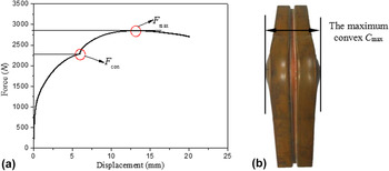
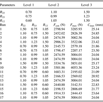
In inverse method, some responses are needed to be determined to quantify the deformation magnitude of DRRT in three-point bending. These responses can track the deformation history (variation of stress and strain for DRRT in three-point bending) and should be easily measured from the test. Bäker and shrot Reference Bäker and Shrot14 pointed out that the deformation history could be considered to be only related to the external force as long as contributions from the boundary conditions are sufficiently small. For three-point bending, just the friction between tube and roller affects the deformation history and the effect is extremely small. So the external force can represent the stress variation of DRRT in three-point bending. Figure 2(a) shows the force–displacement curve of DRRT in three-point bending. It can be seen that the force increases with the downward moving of upper roller and then decreases. The maximum force is denoted as F max. There is a turning point on the curve after which the increasing of force becomes quicker. This is the moment that the ridge groove backs contact with each other. The force in the point is denoted as F con. F con and F max can represent the stress variation of DRRT in three-point bending. Figure 2(b) shows the contour of DRRT after three-point bending. There is a convex in each side of the DRRT after the three-point bending is finished. The maximum convex is denoted as C max and it can be seen as the reflection of strain variation of DRRT in three-point bending. F max and F con can be obtained from the force–displacement curve of DRRT in three-point bending, and C max can be measured on the bent tube by using micrometer. F con, F max, and C max are easily measured from three-point bending, so the three are selected to be used as the responses to quantify the deformation magnitude of DRRT.
The experimental results of three-point bending: (a) force–displacement curve (b) contour of bent DRRT.

C. The procedure of inverse method
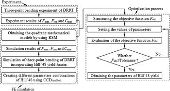
The detailed phases of the inverse methodology incorporating RSM and three-point bending to determine the parameters of Hill’48 yield function, R 22, R 33, and R 12, are shown in Fig. 3. There are three main steps in the proposed inverse method. Firstly, the three-point bending experiment of DRRT was conducted and the experiment results of three responses, F max, F con, and C max, were measured. Then the parameters combination of Hill’48 yield function were created by using central composite design (CCD) algorithm. By using these material data, the FE simulations of three-point bending of DRRT were performed and the simulation results of three responses were obtained. Based on these simulation results, the mathematical models relating the material parameters of Hill’48 yield function to the simulation results of the responses were established by using RSM. The quadratic RSM model is adequate and its polynomial equation is expressed in Eq. (5):
 $${Y_k} = {\beta _0} + \sum\limits_{i = 1}^3 {{\beta _i}{x_i}} + \sum\limits_{i = 1}^3 {{\beta _{ii}}x_i^2} + \sum\limits_{i = 1}^2 {\sum\limits_{j = i + 1}^3 {{\beta _{ij}}{x_i}{x_j}} } \quad ,$$
where Y k is the kth response. β0, β i , β ii , and β ij are the coefficients of intercept, linear, quadratic, and interactive terms, respectively. x i and x j represent the ith and jth parameters of yield function. Finally an objective function defining the gap between the simulation results and experiment ones was structured as shown in Eq. (6) Reference Cao and Lin15 :
 $${F_{{\rm{obj}}}} = {1 \over M}\left[ {\sum\limits_i^M {{w_i}} \cdot {{\left( {{{Y_i^{{\rm{RSM}}} - Y_i^{{\rm{EXP}}}} \over {Y_i^{{\rm{EXP}}}}}} \right)}^2}} \right]\quad ,$$
where
 $Y_i^{\rm RSM}$
represents the response of F
max, F
con, and C
max calculated from mathematical models.
 $Y_i^{\rm EXP}$
is the corresponding values obtained from experiment. M is the number of responses. W
i
is the weight factors representing the relative impact of each term, as shown in Eq. (7):
 $${w_i} = {{Y_i^{{\rm{EXP}}}} \mathord{\left/ {\vphantom {{Y_i^{{\rm{EXP}}}} {\sum\limits_{i = 1}^M {Y_i^{{\rm{EXP}}}} }}} \right. \kern-\nulldelimiterspace} {\sum\limits_{i = 1}^M {Y_i^{{\rm{EXP}}}} }}\quad .$$
Flow chart of the inverse methodology to determine the parameters of Hill’48 yield function.

And then the parameters of Hill’48 yield function were determined by minimizing the objective function in an optimization process.
III. FE MODEL OF THREE-POINT BENDING OF DRRT
In the FE simulation, a material model is needed to be input into the commercial software of ABAQUS and commonly made up of a yield function, strain hardening law, and plastic flow rule. Hill’48 yield function and isotropic hardening law are shown in Eq. (8):
 $$\Phi \left( {\sigma ,{{\bar \varepsilon }^p}} \right) = f\left( \sigma \right) - {\sigma _{\rm{s}}}\left( {{{\bar \varepsilon }^p}} \right) = 0\quad ,$$
where f(σ) is Hill’48 yield function and
 ${\sigma _{\rm{s}}}\left( {{{\bar \varepsilon }^p}} \right)$
is the isotropic hardening law expressed in Eq. (9):
 $${\sigma _{\rm{s}}}\left( {{{\bar \varepsilon }^p}} \right) = k{\left( {{\varepsilon _0} + {{\bar \varepsilon }^p}} \right)^n}\quad ,$$
where
 ${\bar \varepsilon ^p}$
is the equivalent plastic strain. ε0 = 0.0104, K = 588.17 MPa, and n = 0.51 are the material constants of H96 brass DRRT. Other material parameters of H96 brass DRRT such as the elastic modulus and Poisson’s ratio are 92.82 GPa and 0.324, respectively. The associated flow rule is usually adopted, as shown in Eq. (10):
 $$\dot \varepsilon _{ij}^p = \dot \lambda {{\partial f} \over {\partial {\sigma _{ij}}}}\quad ,$$
where
 $\dot \varepsilon _{ij}^p$
is the plastic strain rate,
 ${\sigma _{ij}}$
is the Cauchy stress,
 $\dot \lambda$
is a non-negative scalar called the plastic multiplier.
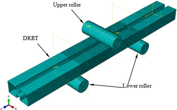
The material model is embedded into the deformable body, DRRT. And DRRT is discretized using 4-node doubly curved thin shell elements S4R. The size of element is 1 × 1 mm. The DRRT located between the two lower rollers is the deformation zone, so this part of DRRT is meshed more finely with the element of 0.8 × 0.8 mm. The rollers are defined as rigid bodies and described by using 4-node 3D bilinear quadrilateral elements C3D4 and the size of element is 2 × 2 mm. The friction between tube and dies is modeled with classical Coulomb friction model and the friction coefficients between tube and dies are 0.05. The degree of freedom of two lower rollers are all restricted. The upper roller is just allowed to move along Y direction. Then the 3D FE model of three-point bending of DRRT was established, as shown in Fig. 4.
The FE model of three-point bending of DRRT.

IV. RESULTS AND DISCUSSION
A. Establishing the mathematical models relating the parameters of Hill’48 yield function to the responses by using RSM
Before establishing the mathematical models relating the parameters of Hill’48 yield function to the responses by using RSM, the FE simulations with different combinations of the three parameters, R 22, R 33, and R 12, are needed to be conducted. To create the different combinations of the three parameters, their approximate ranges should be determined. According to Eq. (4), the values of the three parameters can be determined based on the values of r 0, r 45, and r 90. For small-sized H96 brass DRRT, it is difficult to conduct the uniaxial tensile tests, so the relatively wide ranges (0.5–2) of r 0, r 45, and r 90 are selected. Then the ranges of R 22, R 33, and R 12 were determined, as shown in Eq. (11):
 $$\left\{ {\matrix{ {0.70 \le {R_{22}} \le 1.50} \cr {0.75 \le {R_{33}} \le 1.23} \cr {0.60 \le {R_{12}} \le 1.50} \cr} } \right.\quad .$$
Based on the ranges of the three parameters, each parameter is categorized into three levels, as shown in Table I. According to CCD algorithm, a total of 17 FE simulations of three-point bending were performed to establish the quadratic mathematical models by using RSM. After the FE simulations of three-point bending were performed, the simulation results of three responses, F con, F max, and C max, were recorded in Table I. By using RSM, the quadratic mathematical models relating the parameters of R 22, R 33, and R 12 to the responses were established, as shown in Eqs. (12)–(14):
 $${F_{\max }} = 650.93 - 221.67 \cdot {R_{22}} + 38.74 \cdot {R_{33}} + 823.21 \cdot {R_{12}} + 351.17 \cdot {R_{22}} \cdot {R_{33}} + 599.25 \cdot {R_{22}} \cdot {R_{12}} + 393.50 \cdot {R_{33}} \cdot {R_{12}} + 236.61 \cdot R_{22}^2 - 547.27 \cdot R_{12}^2$$
 $${F_{{\rm{con}}}} = 1568.34 - 24.13 \cdot {R_{22}} - 833.02 \cdot {R_{33}} + 316.74 \cdot {R_{12}} + 1056.20 \cdot {R_{22}} \cdot {R_{33}} + 450.47 \cdot {R_{22}} \cdot {R_{12}} + 771.78 \cdot {R_{33}} \cdot {R_{12}} - 460.95 \cdot R_{12}^2 \cr}$$
 $${C_{\max }} = 13.58 + 14.62 \cdot {R_{22}} - 4.06 \cdot {R_{33}} + 8.30 \cdot {R_{12}} - 5.51 \cdot R_{22}^2 - 3.29 \cdot R_{12}^2$$
Three parameters and experimental matrix for CCD during three-point bending.

The mathematical models generated in RSM must be able to represent the relationship between the parameters of R
22, R
33, and R
12 and the three responses accurately. Thus, 8 different combinations of R
22, R
33, and R
12, which are different from the ones in Table I, were created to evaluate the reliable of the established mathematical models, as shown in Table II. For each parameter combination, the three responses calculated from the mathematical models,
 $F_{\rm con}^{\rm RSM}$
,
 $F_{\rm max}^{\rm RSM}$
, and
 $C_{\rm max}^{\rm RSM}$
, were compared with those obtained from FE simulation,
 $F_{\rm con}^{\rm SIM}$
,
 $F_{\rm max }^{\rm SIM}$
, and
 $C_{\rm max }^{\rm SIM}$
. It can be seen that the average relative errors between the calculated results and the simulation ones for F
con, F
max, and C
max are 0.67%, 0.61%, and 1.15%, respectively. Thus, the mathematical models in Eqs. (12)–(14) are reliable. And then the mathematical models were substituted into Eq. (6) to construct the objective function. The parameters of Hill’48 yield function, R
22, R
33, and R
12, can be determined by minimizing the objective function.
8 different combinations of R 22, R 33, and R 12 and the comparisons of the responses obtained from FE simulation and the mathematical models.

B. The reliability of the proposed inverse method of identifying the parameters of Hill’48 yield function
1. The comparison of different yield functions in describing the anisotropy of H96 brass DRRT
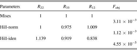
For an anisotropic yield function, it is important to have the ability of describing the anisotropy of material. Table III shows the parameters of three yield functions, Hill’48 yield function with the identified parameters denoted as “Hill-iden”, Hill’48 yield function only considering the normal anisotropy denoted as “Hill-norm” and Mises yield function. When the parameters of Hill’48 yield function, R 22, R 33, and R 12, are set equal to 1, the anisotropic Hill’48 yield function is degraded to Mises yield function. For “Hill-norm”, r 45 and r 90 are set equal to r 0 and the parameters of R 22, R 33, and R 12 were obtained according to Eq. (4). The parameters of R 22, R 33, and R 12 for “Hill-iden” are obtained by the inverse method. It can be seen that “Hill-norm” takes the anisotropy of material into account, but the values of R 22, R 33, and R 12 for “Hill-norm” are approximate to 1 without obvious anisotropy. For “Hill-iden”, the values of R 22, R 33, and R 12 are quite different and present more obvious anisotropy. Meanwhile, the objective function values F obj for the three yield functions were calculated according to Eq. (6), as shown in Table III. It can be seen that F obj for “Hill-norm” and Mises yield function is relative large, which indicates that the simulation results obtained by using the two yield functions are quite different from those obtained from experiment. But F obj for “Hill-iden” is extremely small and reduces about 98.54% compared to “Hill-norm”. Thus, it is indicated that “Hill-iden” can describe the anisotropic behaviors of H96 brass DRRT more accurately.
The parameters of different yield functions.

2. Evaluating the reliability of the proposed inverse method
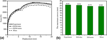
To evaluate the reliability of the proposed inverse method of identifying the parameters of Hill’48 yield function, the FE simulations of three-point bending of H96 brass DRRT with the three yield functions were conducted and the force–displacement curves obtained from simulations were compared with the experimental one, as shown in Fig. 5(a). It can be seen that the force–displacement curve obtained from simulation by using Mises yield function is quite different that obtained from experiment. By using “Hill-norm”, the prediction accuracy of force–displacement curve is improved, but the relative errors for F con and F max between experiment and simulation are still large, about 3.71% and 2.76%, respectively. When “Hill-iden” is used in the simulation of three-point bending of DRRT, the relative errors for F con and F max between experiment and simulation are reduced to 0.03% and 0.02%, respectively. Besides, the relative error for maximum convex C max between experiment and simulation is about 4.31% when the “Hill-norm” is used. When the “Hill-iden” is used, the relative error for C max between experiment and simulation is reduced to 1.17%, as shown in Fig. 5(b). So it can be concluded that the deformation behaviors of H96 brass DRRT in three-point bending can be simulated by Hill’48 yield function with the identified parameters more accurately.
The comparison of FE simulation results using different yield criteria and experimental results: (a) displacement–load curves (b) the maximum convex.

V. APPLICABILITY OF THE INVERSE METHOD IN ROTARY DRAW BENDING OF DRRT
A. The rotary draw bending of DRRT
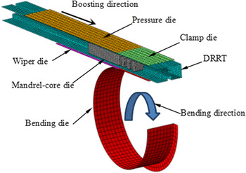
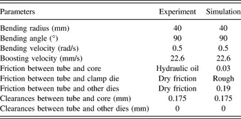
To evaluate the applicability of the proposed inverse method in real forming process, the rotary draw bending of H96 brass DRRT was carried out. The FE model of rotary draw bending of DRRT with a dynamic explicit code was established on the platform of ABAQUS, as shown in Fig. 6. The dies were modeled with 4-node 3D bilinear quadrilateral elements C3D4. The DRRT is deformable body and it was meshed with 4-node doubly curved thin shell elements S4R. The friction between tube and dies is modeled with classical Coulomb friction model. The FE simulations of rotary draw bending of DRRT with the Hill’48 yield function obtained by the inverse method, Hill’48 yield function only considering the normal anisotropy and Mises yield function were carried out. The process parameters of rotary draw bending of DRRT in FE simulation and experiment are shown in Table IV.
The FE model of rotary draw bending of DRRT.

The process parameters of rotary draw bending of DRRT.

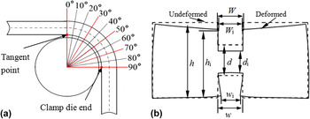
To measure the cross sectional deformation of DRRT along bending direction, ten cross sections distributed evenly in the zone of 0°–90° were selected in FE simulation and five cross sections of 0°, 30°, 50°, 70, and 90° were selected in experiment, as shown in Fig. 7(a). In Fig. 7(b), four responses, flange sagging Δh, space deformation between ridges Δd and width deformation of outer and inner ridge grooves ΔW and Δw, are selected to characterize the cross sectional deformation of DRRT, as shown in Eqs. (15)–(18):
 $$\Delta h = {{{h_i} - h} \over h} \times 100\%$$
 $$\Delta d = {{{d_i} - d} \over d} \times 100\%$$
 $$\Delta w = {{{w_i} - w} \over w} \times 100\%$$
 $$\Delta W = {{{W_i} - W} \over W} \times 100\% \quad ,$$
where h, d, W, and w are the values of section height, space between ridges, outer ridge groove width, and inner ridge groove width before bending deformation. h i , d i , W i , and w i are the corresponding values after bending deformation.
The selection of typical cross sections and indexes to characterize the cross sectional deformation: (a) typical cross sections (b) typical nodes and indexes.

B. Results and discussions
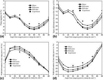
Figure 8 shows the cross sectional deformation of DRRT along bending direction obtained from experiment and FE simulations with the three yield functions. The negative values represent that the values of cross sectional deformation after deformation is smaller than that before deformation. From Fig. 8, it can be seen that the cross sectional deformation of DRRT was overestimated by the FE simulations with the Mises yield function. The error of cross sectional deformation between the simulation by using Mises yield function and experiment is relative large. The error of cross sectional deformation between the simulation by using “Hill-norm” is reduced but only a little. When “Hill-norm” is used, the average errors between the simulation and experiment for flange sagging Δh, space deformation between ridges Δd and width deformation of outer and inner ridge groove ΔW and Δw are 17.70%, 20.12%, 18.28%, and 21.89%, respectively. But when “Hill-iden” is used, the average errors between the simulation and experiment for Δh, Δd, ΔW, and Δw decrease to 11.51%, 9.49%, 11.42%, and 10.34%, respectively. It is indicated that when the Hill’48 yield function with the identified parameters was used in the FE simulation of rotary draw bending of DRRT, the prediction accuracy of Δh, Δd, ΔW, and Δw were improved 6.19%, 10.63%, 6.86%, and 11.55%, respectively, compared to that by using the Hill’48 yield function only considering the normal anisotropy.
The cross sectional deformation of DRRT along bending direction obtained from experiment and FE simulations with different yield functions: (a) flange sagging (b) space deformation of between ridges (c) width deformation of outer ridge groove (d) width deformation of inner ridge groove.

VI. CONCLUSION
-
(1) An inverse parameter identification method combining response surface methodology and three-point bending was proposed to determine the parameters of Hill’48 yield function. By using the proposed inverse method, the material behaviors of H96 brass DRRT in bending process, which is difficult to be obtained based on the standard tests, can be obtained. In addition, this inverse method can avoid the iterative conducting of FE simulations, which highly reduces the computing time.
-
(2) Comparing with Hill’48 yield function only considering the normal anisotropy and Mises yield function, Hill’48 yield function with the identified parameters performs the best in reproducing the material behavior of H96 brass DRRT in three-point bending process. When Hill’48 yield function with the identified parameters was used in the FE simulation of rotary draw bending of DRRT, the prediction accuracies of flange sagging Δh, space deformation between ridges Δd and width deformation of outer and inner ridge grooves ΔW and Δw were improved 6.19%, 10.63%, 6.86%, and 11.55%, respectively, compared with that when Hill’48 yield function only considering the normal anisotropy was used.
ACKNOWLEDGMENTS
The authors would like to thank the National Natural Science Foundation of China (No. 51375392) and the Research Fund of the State Key Laboratory of Solidification Processing (NWPU), China (No. 152-ZH-2016) for the support given to this research.