

1. Introduction
Of particular importance to mixing enhancement design in any combustion device is the satisfactory prediction of the time that it takes fuel to achieve a well-mixed state. Among all combustion propulsion-based strategies, mixing enhancement in supersonic flows of a scramjet is a notoriously challenging problem owing to the extremely short residence time for mixing. A prototype of shock-enhanced mixing was first proposed by Marble, Hendricks & Zukoski (Reference Marble, Hendricks and Zukoski1989), and it offered a new way of using the shock-induced streamwise vortex formed from the baroclinic vorticity production through an oblique shock/jet interaction to enhance mixing in a supersonic flow (Waitz, Marble & Zukoski Reference Waitz, Marble and Zukoski1993). The streamwise vortex not only avoids the disadvantage of reduced mixing for parallel fuel injection from the Kelvin–Helmholtz instability at high convective Mach number (Curran, Heiser & Pratt Reference Curran, Heiser and Pratt1996), but also has the potential to shorten the length of the scramjet combustor (Chan Reference Chan2010) owing to the rapid mixing rate. Thus, understanding the effect of a supersonic streamwise vortex on mixing is vital for mixing enhancement in the scramjet.
Studying the mixing enhancement mechanisms under a supersonic streamwise vortex suffers from complexity of three-dimensional (3-D) flow structures such as shock-wave structures and the density gradient between fuel and ambient air (Urzay Reference Urzay2018). Therefore, passive mixing and pseudo-combustion behaviour in the flow field of an ideal Lamb–Oseen-type vortex was pioneeringly studied by Marble (Reference Marble1985). An unsteady mixing process, as well as diffusion flame growth, is a combined effect of advection and diffusion control based on the defined Péclet number,  $Pe=\varGamma /\mathscr {D}$, where
 $\varGamma$ is the circulation of a streamwise vortex and
 $\mathscr {D}$ is the scalar diffusivity. Cetegen & Mohamad (Reference Cetegen and Mohamad1993) conducted a series of experimental studies in water to produce a single two-dimensional vortex with scalar concentration. The mixing indicator ‘mixedness’ was proposed to study the mixing enhancement extent, which is defined as
 $f=4c(1-c)$ where
 $c$ is the scalar concentration. It was found that the mixedness grows linearly with the total circulation of the vortex, and the scalar dissipation follows this trend as well, which shows a derivative relationship between mixedness and scalar dissipation. Basu, Barber & Cetegen (Reference Basu, Barber and Cetegen2007) further studied the scalar mixing in the gaseous laminar line vortex. Empirical correlations considering the variable temperature ratio, circulation strength and time of interaction were built. The systematic research of mixing time in a point vortex was further extended by Meunier & Villermaux (Reference Meunier and Villermaux2003) who theoretically pointed out the critical dependence of mixing time to decay a passive scalar on 1/3 scaling of
 $Pe$. Sau & Mahesh (Reference Sau and Mahesh2007) conducted the first DNS simulation of passive-scalar (PS) mixing in a 3-D vortex ring. The optimal mixing from a vortex ring was also confirmed when the vortex grew to pinch-off status (Gharib, Rambod & Shariff Reference Gharib, Rambod and Shariff1998), which was recently also validated in the formation of a supersonic vortex ring (Lin et al. Reference Lin, Xiang, Xu, Liu and Zhang2020; Qin et al. Reference Qin, Xiang, Lin and Liu2020). Such a simple PS mixing protocol offers ample phenomena that are resolvable to a near-exact solution, which attracts researchers and provides more in-depth mechanisms of stretching-enhanced diffusion characteristic of mixing (Villermaux Reference Villermaux2019).
The PS mixing behaviour in a vortical flow has been applied in the design of a lobed mixer (Waitz et al. Reference Waitz1997) or a strut mixer (Vergine, Ground & Maddalena Reference Vergine, Ground and Maddalena2016), which generates the interacting streamwise vortices to enhance mixing (Wang et al. Reference Wang, Yu, Zhang, He and Liu2021). It is noteworthy that the flow inside scramjet combustors invariably involves inhomogeneous compressible mixing. Therefore, it is desirable to understand the role that the density difference (Schetz, Maddalena & Burger Reference Schetz, Maddalena and Burger2010) and shock compression (Tew, Hermanson & Waitz Reference Tew, Hermanson and Waitz2004) play in mixing enhancement. Furthermore, whether an understanding of the variable-density (VD) effect will lead to the better control of a shock-enhanced mixing strategy is still an open question. To simplify the streamwise vortex production from a shocked VD jet, Yang, Kubota & Zukoski (Reference Yang, Kubota and Zukoski1994) proposed that the steady 3-D jet–shock interaction can be an analogy to a simple two-dimensional unsteady shock–bubble interaction (SBI) under the slender body approximation. If the supersonic inflow is high enough ( $Ma>3$) that the spanwise velocity is much smaller than the streamwise velocity, the dynamics of spanwise flow can be related to a two-dimensional SBI (Yu et al. Reference Yu, He, Zhang and Liu2020; Zhang et al. Reference Zhang, Liu, Yu, Wang, He and Liu2021). More importantly, an SBI is a canonical prototype of Richtmyer–Meshkov instability (RMI), which is a fascinating research field to investigate the fundamental VD mixing problem in shock-accelerated flows (Brouillette Reference Brouillette2002; Ranjan, Oakley & Bonazza Reference Ranjan, Oakley and Bonazza2011). Hence, an SBI is a suitable research target to study the vortical mixing behaviour under the condition of the compressible and VD environment.
After shock passage across a bubble, baroclinic vorticity is formed by the misalignment of the density gradient and pressure gradient, which enhances mixing between the density inhomogeneity (Zabusky Reference Zabusky1999). Delicate vortex formation and mixing evolution appear in the SBI (Ranjan et al. Reference Ranjan, Niederhaus, Oakley, Anderson, Bonazza and Greenough2008). Despite such simple initial conditions, a wealth of physical phenomena still occur and have been studied numerically (Quirk & Karni Reference Quirk and Karni1996) and experimentally (Layes, Jourdan & Houas Reference Layes, Jourdan and Houas2003). The secondary vortex ring in the shock–light bubble interaction (Ranjan et al. Reference Ranjan, Niederhaus, Motl, Anderson, Oakley and Bonazza2007) and the late time turbulence behaviour in the shock–heavy bubble interaction (Ranjan et al. Reference Ranjan, Anderson, Oakley and Bonazza2005; Niederhaus et al. Reference Niederhaus, Greenough, Oakley, Ranjan, Anderson and Bonazza2008) are found continuously. Moreover, owing to the characteristic of the vortex structure, much focus has been placed on building the circulation model in the study of SBI (Picone & Boris Reference Picone and Boris1988; Samtaney & Zabusky Reference Samtaney and Zabusky1994; Yang et al. Reference Yang, Kubota and Zukoski1994; Niederhaus et al. Reference Niederhaus, Greenough, Oakley, Ranjan, Anderson and Bonazza2008; Liu et al. Reference Liu, Yu, Chen, Zhang, Xu and Liu2020b) and the related shock dynamics of the SBI (Zhai et al. Reference Zhai, Si, Luo and Yang2011; Luo et al. Reference Luo, Wang, Si and Zhai2015; Si et al. Reference Si, Long, Zhai and Luo2015; Ding et al. Reference Ding, Si, Chen, Zhai, Lu and Luo2017; Igra & Igra Reference Igra and Igra2020).
As for the mixing studies of an SBI, two crucial characteristics of the mixing behaviour have been studied. The first is to measure the extent of stirring mixing arising from the vortex stretching, such as mass fraction contour area and material stretching rate. Pioneering experimental work conducted by Marble et al. (Reference Marble, Zukoski, Jacobs, Hendricks and Waitz1990) showed that the mixing of the distorted bubble became stable at approximately 1 ms under the weak shock condition ( $Ma=1.1$). They proposed a characteristic scaling time based on dimensional analysis as
 $D^2/\varGamma \sim D/[c_0(Ma^2-1)]$ (
 $c_0$ is the sound speed,
 $D$ is the bubble diameter and
 $\varGamma$ is the vortex circulation), which demonstrated that a small increase of the shock strength will lead to a large reduction of the mixing time. Further, Jacobs (Reference Jacobs1992) experimentally measured the mass fraction contour area by using the planar laser-induced fluorescence (PLIF) technique for the first time. The mixing is controlled by the dimensionless time,
 $\varGamma ^{{2}/{3}}\mathscr {D}^{{2}/{3}}t/D^2$, proposed from PS mixing by Marble (Reference Marble1985). It was found that the mixing owing to a vortex will happen at a faster rate before a dimensionless time of 0.25 is reached. The stretching rate of the material line contour (Yang, Kubota & Zukoski Reference Yang, Kubota and Zukoski1993) is a pervasive method to render the spatial mixing measurement and presents the exponent growth of the material line at the incipient stage after shock. However, the material line contour is valid and the material stretching rate is appropriate only when the boundary of the mass fraction contour is clearly recognised (Kumar et al. Reference Kumar, Orlicz, Tomkins, Goodenough, Prestridge, Vorobieff and Benjamin2005), i.e. dimensionless time
 $c_0t/R<50$ (
 $R$ is the radius of the bubble). The second is to measure the extent of the molecular diffusion mixing in the presence of the baroclinic vortex formed by shock impact. The scalar dissipation caused by a concentration gradient has been examined in SBI mixing by detailed PLIF measurement (Tomkins et al. Reference Tomkins, Kumar, Orlicz and Prestridge2008). The stable region, such as bridge structures, tends to be the high-mixing-rate contributor. Interestingly, the unstable region, such as a vortex formed after the shock impact and secondary instabilities, offers less mixing than the stable region owing to the high strain in the bridge structure. Mixing time was also estimated by the theory proposed by Marble (Reference Marble1985) and it was concluded that mixing continues inside the theoretical prediction.
It is noteworthy that significant progress has been achieved in the past 15 years in RMI theories (see Thornber et al. Reference Thornber, Drikakis, Youngs and Williams2010; Hahn et al. Reference Hahn, Drikakis, Youngs and Williams2011; Thornber et al. Reference Thornber, Drikakis, Youngs and Williams2011; Zhou et al. Reference Zhou2021 and references therein), which is beneficial to understand the SBI mixing mechanism. Vorobieff et al. (Reference Vorobieff, Rightley and Benjamin1998) found that a mixing transition happens in a shock–gas curtain interaction when a dimensionless time  $u_1't/\lambda \approx 6.6$ is achieved (
 $u_1'$ is the post-shock gas speed and
 $\lambda$ is the perturbation wavelength of the gas curtain). Following Vorobieff et al. (Reference Vorobieff, Rightley and Benjamin1998), Niederhaus et al. (Reference Niederhaus, Greenough, Oakley, Ranjan, Anderson and Bonazza2008) investigated typical SBI cases under dimensionless time
 $u_1't/R$, which scales the mixing process under different shock Mach numbers in one gas pair. Recently, based on impulsive model from Richtmyer (Reference Richtmyer1960), Oggian et al. (Reference Oggian, Drikakis, Youngs and Williams2015) found that self-similar growth is obtained at
 ${At}^+\Delta ut/\lambda _{min}\approx 250$ in multi-mode RMI (
 ${At}^+$ is the post-shock Atwood number,
 $\Delta u$ is velocity impulse imparted by shock and
 $\lambda _{min}$ is the minimal wavelength of the perturbed interface), in accordance to the simulations from Lombardini, Pullin & Meiron (Reference Lombardini, Pullin and Meiron2012).
Table 1 summarises the mixing behaviour of different cases from the literature investigating the shock-accelerated flows. It can be found that the definition of mixing time that is widely accepted and well predictable is absent in shock-accelerated VD mixing. Dimensionless times, related to post-shock velocity, are able to scale the temporal mixing width or bubble morphology evolution, while they lack the inherent expression of mixing behaviour, i.e. diffusivity  $\mathscr {D}$. The mixing time proposed by Marble (Reference Marble1985) and Meunier & Villermaux (Reference Meunier and Villermaux2003), who considered the PS mixing characteristic, can hardly predict the mixing time of the concentration decay in the VD SBI, as analysed in the present paper. Although the time-scaling dependence on Mach number proposed by Marble et al. (Reference Marble, Zukoski, Jacobs, Hendricks and Waitz1990) is beneficial in preliminary mixing enhancement design, its theoretical basis is still the PS mixing, which omits the VD contribution to the mixing enhancement. We will show that a coupling mechanism from the VD characteristic and the shock compression (Giordano & Burtschell Reference Giordano and Burtschell2006) can offer a well-posed mixing time prediction for SBI.
The mixing behaviour of shock-accelerated flows from different studies under different dimensionless times.

In this work, we are devoted to understand and reveal the effect of secondary baroclinic vorticity (SBV), which is ubiquitous in VD flows, on mixing enhancement. By focusing on the shock–helium bubble interaction in a wide range of shock Mach numbers from 1.22 to 4, a VD SBI and a PS counterpart are compared for the first time to show the importance of SBV-accelerated stretching on the mixing behaviour. Based on solving the advection–diffusion equation under a deformation field of an axisymmetric vortex with the additional SBV-increased azimuthal velocity, a theoretical model for mixing time estimation is proposed. This model reveals the role that density difference plays in shock-accelerated inhomogeneity mixing. Our results provide insights into the nature and mechanisms of VD mixing in general and yields the direction for predicting a well-mixed state in supersonic flows.
The organisation of the present paper is as follows: The governing equations and numerical set-up are introduced in § 2. The vortex formation after the shock impact on the bubble and the mixing process of both VD SBI and PS SBI are examined in § 3. Section 4 introduces the mechanism of the baroclinic accelerated stretching. Based on the analysis on the baroclinicity, the characteristic time for mixing enhancement is derived for both PS SBI and VD SBI in § 5. Further, a mixing enhancement number is proposed to illustrate the contribution from the VD effect in § 6. Important conclusions are summarised in § 7.
2. Numerical approach and set-up
2.1. Governing equations and numerical method
The multi-component flows concerned in the present study are two-dimensional shock–cylindrical bubble interactions. The two-dimensional compressible Navier–Stokes (N–S) equations with multi-components are as follows:
 \begin{equation} \frac{\partial \boldsymbol{U}}{\partial t}+\frac{\partial \boldsymbol{F}}{\partial x} +\frac{\partial \boldsymbol{G}}{\partial y} =\frac{\partial \boldsymbol{F}_{v}}{\partial x}+\frac{\partial \boldsymbol{G}_{v}}{\partial y}, \end{equation}
where vector  $\boldsymbol {U}$ is the conserved term and vectors
 $\boldsymbol {F}$,
 $\boldsymbol {G}$ and
 $\boldsymbol {F}_{v}$,
 $\boldsymbol {G}_{v}$ represent the convection and diffusion terms, respectively. The vectors are given by
 \begin{equation} \left.\begin{array}{l} \boldsymbol{U}=[\rho,\rho u,\rho v,\rho e_0,\rho Y_1,\ldots\rho Y_{NS-1}]^\textrm{T},\\ \boldsymbol{F}=[\rho,\rho u^2+p,\rho uv,(\rho e_0+p)u,\rho_1 u,\ldots\rho_{NS-1}u]^\textrm{T},\\ \boldsymbol{G}=[\rho,\rho uv,\rho v^2+p,(\rho e_0+p)v,\rho_1 v,\ldots\rho_{NS-1}v]^\textrm{T},\\ \boldsymbol{F}_v=\left[0,\tau_{xx},\tau_{xy},u\tau_{xx}+v\tau_{xy}-q_x, -\rho \mathscr{D}_1\dfrac{\partial Y_1}{\partial x},\ldots -\rho \mathscr{D}_{NS-1}\dfrac{\partial Y_{NS-1}}{\partial x}\right]^\textrm{T},\\ \boldsymbol{G}_v=\left[0,\tau_{xy},\tau_{yy},u\tau_{xy}+v\tau_{yy}-q_y, -\rho \mathscr{D}_1\dfrac{\partial Y_1}{\partial y},\ldots -\rho \mathscr{D}_{NS-1}\dfrac{\partial Y_{NS-1}}{\partial y}\right]^\textrm{T}, \end{array}\right\} \end{equation}
where  $\rho,p,e_0$ represent the mixture's density, pressure and the total energy per unit mass, respectively,
 $u,v$ are the speeds of the mixture,
 $\rho _i$ and
 $Y_i$ denote the density and mass fraction of the species
 $i$, and
 $NS$ denotes the total number of species. The viscous tensor
 $\tau$ and heat flux
 $q$ are defined as
 \begin{equation} \left.\begin{array}{l} \tau_{xx}=\dfrac{2}{3}\mu\left( 2\dfrac{\partial u}{\partial x}-\dfrac{\partial v}{\partial y}\right),\\ \tau_{yy}=\dfrac{2}{3}\mu\left(2\dfrac{\partial v}{\partial y}-\dfrac{\partial u}{\partial x}\right),\\ \tau_{xy}=\mu\left(\dfrac{\partial u}{\partial y}+\dfrac{\partial v}{\partial x}\right), \end{array}\right\}\quad\textrm{and} \quad \begin{array}{l} q_x=\lambda\dfrac{\partial T}{\partial x} +\rho\displaystyle\sum_{i=1}^{NS}\mathscr{D}_i h_i\dfrac{\partial Y_i}{\partial x},\\ q_y=\lambda\dfrac{\partial T}{\partial y} +\rho\displaystyle\sum_{i=1}^{NS}\mathscr{D}_i h_i\dfrac{\partial Y_i}{\partial y}, \end{array} \end{equation}
in which  $T$ is the temperature and
 $h_i$ is the specific enthalpy of species
 $i$. Here,
 $\mu,\lambda$ are the dynamic viscosity and thermal conductivity of the mixed gas, given by Wike's semi-empirical formula (Gupta, Yos & Thompson Reference Gupta, Yos and Thompson1989). For high-speed flow numerical simulations, mass diffusion can be simplified by ignoring pressure and temperature diffusion, and it is assumed to be constant for different components:
 \begin{equation} \mathscr{D}_i=\mathscr{D}=\frac{\mu}{\rho Sc}. \end{equation}
Moreover, the Schmidt number is assumed as constant  $Sc=0.5$ (Gupta et al. Reference Gupta, Yos and Thompson1989). For the thermal conductivity,
 $\lambda$ is calculated from the Prandtl number as
 $Pr=0.72$ (Houim & Kuo Reference Houim and Kuo2011). To close the system of equations, the equation of ideal gas state is needed:
 \begin{equation} p=\rho R_u T\sum_{i=1}^{NS}\frac{Y_i}{M_i}, \end{equation}
where  $R_u$ is the ideal gas constant and
 $M_i$ is the molar mass of component
 $i$. The total energy
 $e_0$, which contains the specific internal energy
 $e$ and kinetic energy, is given by
 \begin{equation} e_0=e+\frac{1}{2}(u^2+v^2)=h-\frac{p}{\rho}+\frac{1}{2}(u^2+v^2). \end{equation}
Here,  $h$ is the specific enthalpy of the gas mixture,
 \begin{equation} h=\sum_{i=1}^{NS}Y_i h_i=\sum_{i=1}^{NS}Y_i\left(h_{fi}^0+\int_{T_0}^{T}\frac{C_{pi}}{M_i}\,\mathrm{d}T\right), \end{equation}
in which  $h_{fi}^0$ is the heat generated by the component
 $i$ at the reference temperature
 $T_0$. The constant-pressure specific heat value
 $C_{pi}$ is fitted by the following temperature-dependent polynomial function:
 \begin{equation} C_{pi}=R_u(a_{1i}+a_{2i}T+a_{3i}T^2+a_{4i}T^3+a_{5i}T^4), \end{equation}
where the coefficients  $a_{1i},\ldots,a_{5i}$ can be obtained from the NASA thermochemical polynomial fit coefficient data (Kee et al. Reference Kee, Rupley, Meeks and Miller1996). After the mathematical model is non-dimensionalised, the finite volume method is used for discretisation. Time is marched by the third-order total variation diminishing (TVD) Runge–Kutta method (Gottlieb & Shu Reference Gottlieb and Shu1998); convection terms are discretised using the fifth-order weighted essentially non-oscillatory (WENO) scheme (Liu, Osher & Chan Reference Liu, Osher and Chan1994; Jiang & Shu Reference Jiang and Shu1996), while viscous terms are discretised by using the central difference method. The general platform of the high-resolution calculation method in the present study is implemented as in-house code ParNS, which has been validated in our previous work and is suitable for this study (Wang et al. Reference Wang, Yu, Chen, Zhang and Liu2018; Li et al. Reference Li, Wang, Yu, Zhang and Liu2020; Liu et al. Reference Liu, Wang, Yu, Zhang and Liu2020a). Moreover, the numerical uncertainty originating from different WENO schemes is essential to capture the physical values, which is discussed in Appendix B.
2.2. Initial conditions for VD SBI
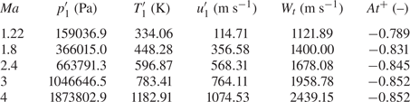
The schematic of the initial conditions of VD SBI is depicted in figure 1. The cylindrical bubble is filled with pure helium. A wide range of shock  $Ma$ number cases (
 $Ma = 1.22$ to 4) are simulated. Same pre-shock conditions for all cases are quiescent air at
 $p_1=1\,01\,325$ Pa and
 $T_1=293$ K. The detailed initial conditions for post-shock air, obtained from one-dimensional (1-D) shock dynamics, are listed in table 2. To avoid spurious vorticity generated by the mesh discretisation (Niederhaus et al. Reference Niederhaus, Greenough, Oakley, Ranjan, Anderson and Bonazza2008), we set the initial interface of the cylindrical bubble smoothed by a diffuse interfacial transition layer defined as
 \begin{equation} Y_{He}(r)=\left\{ \begin{array}{ll} Y_{max} & {r\leq{R}}, \\ Y_{max}\,\mathrm{e}^{-\alpha[(r-R)/\delta]^2} & {R< r\leq{R+\delta}}, \\ 0 & r>R+\delta, \end{array}\right. \end{equation}
where  $\delta /R=0.15$,
 $\alpha =5$ and
 $R=2.6$ mm. Because the reflecting shock from the top wall will influence the cylindrical bubble formation and mixing process, we mainly focus on the mixing mechanism from the once-shocked interface in a shock-free environment. Thus, the interpolation boundary conditions are chosen at the top and two sides of the computational domain. The centreline is chosen as the symmetry boundary condition. The calculation domain in the streamwise direction
 $L=32R$ (
 $R$ is the radius of the cylindrical bubble) is longer than that in most other studies to study the long time evolution of bubble deformation and mixing growth. The calculation domain in the spanwise direction
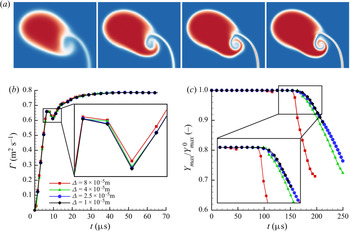
 $H=3R$ is sufficient to avoid reflected waves from the upper side. The mesh independence study can be found in Appendix A. Here, using the mesh resolution
 $\varDelta =2.5\times 10^{-5}$ m leads to grid independence for the problem studied in this paper.
Schematic of the initial conditions for SBI.

Parameters for different shock Mach number cases, including post-shock pressure  $p_1'$, post-shock temperature
 $T_1'$ and the transmitted shock wave speed
 $W_t$, calculated from 1-D gas dynamics. Post-shock Atwood number
 ${At}^+=(\rho _2'-\rho _1')/(\rho _2'+\rho _1')$ is obtained from the post-shock air density
 $\rho _1'$ and post-shock helium density
 $\rho _2'$.

2.3. Initial conditions for PS SBI
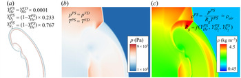
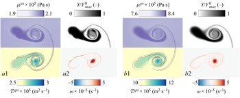
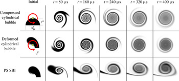
To study the VD effect on mixing, we set a counterpart of the PS SBI without density gradient to be compared with the original VD SBI. One needs to maintain the same circulation, compression and diffusivity as the SBI cases except that the density should be the same as the shocked ambient air to illustrate the PS mixing under a vortical flow. In that scenario, the density effect can be nearly ignored when the vortex grows, and the mixing process will not alter the flow dynamics as PS mixing (Dimotakis Reference Dimotakis2005). However, if a PS bubble is set before the shock impact, no vorticity will be deposited along the bubble interface owing to the absence of a density gradient between the cylindrical bubble and ambient air, which is essential for the baroclinic vorticity production. Thus, a natural selection is to artificially make the cylindrical bubble's mass component equal to the air immediately after the shock impact, so the bubble density will increase to the value of the shocked air. Moreover, a small amount of helium is maintained to reflect the scalar mixing:
 \begin{equation} \left.\begin{array}{l@{}} Y_{He}^{ps}=Y_{He}^{vd}\times 0.0001 , \\ Y_{O_2}^{ps}=(1-Y_{He}^{ps})\times 0.233,\\ Y_{N_2}^{ps}=(1-Y_{He}^{ps})\times 0.767. \end{array}\right\} \end{equation}
If pressure and temperature are set to be the same as the VD SBI case, one obtains
 \begin{equation} \left.\begin{array}{l@{}} p^{ps}=p^{vd},\\ T^{ps}=T^{vd}. \end{array}\right\} \end{equation}
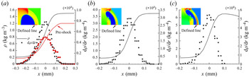
Then, the bubble density will rise to a value similar to the shocked air, as shown in figure 2, where
 \begin{equation} \rho^{ps}=\frac{p^{ps}}{R_gT^{ps}}\approx \rho_{air} \quad \textrm{and}\quad R_g=R_u \sum_{i=1}^{NS}\frac{Y_i^{ps}}{M_i}. \end{equation}
This set of values of  $p,\rho,T$ and
 $Y_i$ comprise the initial conditions for the PS SBI. The calculation of the PS bubble diffusivity is introduced separately in Appendix C to meet the requirement of the same level of diffusivity with a VD bubble. The discretised version of N–S equations (2.1) are then solved numerically in the same way as introduced in § 2.1. The flow will evolve without an evident density gradient owing to the low concentration of helium.
Initial conditions for PS SBI shown by (a) isolines of mass fraction, (b) pressure contour and (c) density contour at  $t=7.2$
 $\mathrm {\mu }$s of the
 $Ma=2.4$ case.

Because the PS mixing obeys the advection–diffusion equation (Villermaux Reference Villermaux2019), which is different from species transport in the N–S equations (2.1), we here prove that if the density gradient can be eliminated, the multi-components transport equations can degenerate to the advection–diffusion equation, which offers the basis for studying the PS mixing of an SBI. Referring back to (2.1), the multi-components transport equations for an arbitrary component follow Fickian's law of diffusion, which can be expressed as
 \begin{equation} \frac{\partial(\rho Y_s)}{\partial t}+\frac{\partial(\rho u_j Y_s)}{\partial x_j}=\frac{\partial}{\partial x_j} \left(\rho\mathscr{D} \frac{\partial Y_s}{\partial x_j} \right). \end{equation}
When assuming constant diffusion, it can be further derived as
 \begin{equation} Y_s\left(\frac{\partial\rho}{\partial t}+\frac{\partial (\rho u_j) }{\partial x_j}\right)+ \rho\left(\frac{\partial Y_s}{\partial t}+u_j\frac{\partial Y_s}{\partial x_j}-\mathscr{D}\frac{\partial^2 Y_s}{\partial x_j^2}\right)=\mathscr{D}\frac{\partial Y_s}{\partial x_j}\frac{\partial\rho}{\partial x_j}. \end{equation}
Owing to the conservation of mass, the term of the first parenthesis is zero, then we obtain
 \begin{equation} \frac{\partial Y_s}{\partial t}+u_j\frac{\partial Y_s}{\partial x_j}-\mathscr{D}\frac{\partial^2 Y_s}{\partial x_j^2}= \frac{\mathscr{D}}{\rho} \left(\frac{\partial Y_s}{\partial x_j}\frac{\partial\rho}{\partial x_j}\right). \end{equation}
Thus, when the density gradient  $\boldsymbol {\nabla }\rho$ is negligible, the species equation can degenerate to the standard advection–diffusion equation.
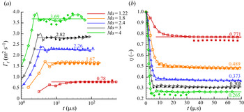
To check whether the circulation and compression are the same as in the VD cases, we compare these two variables between PS SBI and VD SBI, as shown in figure 3. The total circulation is calculated as
 \begin{equation} \varGamma_t=\int_{Y_{He}<1\,\%Y_{max}} \omega \,\textrm{d}V, \end{equation}
where  $\omega$ is the magnitude of the vorticity vector
 $\boldsymbol {\omega }=\boldsymbol {\nabla }\times \boldsymbol {u}$. The compression rate is calculated as (Giordano & Burtschell Reference Giordano and Burtschell2006)
 \begin{equation} \eta=\frac{\int \mathcal{V}_{He}\,\textrm{d}V}{\mathcal{V}_0}\equiv\frac{\mathcal{V}_b}{\mathcal{V}_0}, \end{equation}
where  $\mathcal {V}_{He}$ is the volume fraction of the helium cylindrical bubble and
 $\mathcal {V}_b$ is the volume of a compressed cylindrical bubble. For the initial volume of the PS bubble
 $\mathcal {V}_0$, it is calculated in the same way by decreasing the helium mass fraction multiplied by 0.0001. Figure 3 shows that a higher shock Mach number leads to higher circulation and a lower compression rate. The circulation and compression for both PS SBI and VD SBI are nearly the same, which facilitates the study of the VD effect on the mixing behaviour. The fluctuation of the circulation magnitude at a late time, especially for high Mach number, is because the boundary chosen based on the mass fraction threshold contains negative vorticity forming from the slipstream of the triple point of the Mach stem. However, this negative vorticity has little effect on mixing.
Comparison of circulation (a) and compression rate (b) for PS (solid points) and VD SBI (hollow points) for different shock Mach number cases.

3. Faster mixing decay in VD SBI
3.1. Temporal evolution of cylindrical bubble morphology
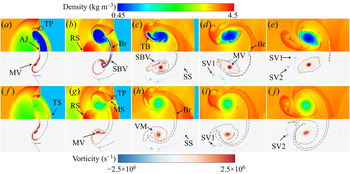
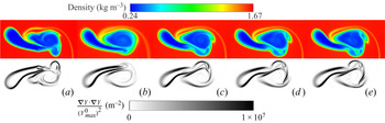
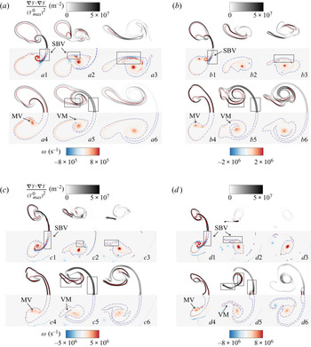
The temporal evolution of the shocked cylindrical bubble morphology is generally similar for different shock strengths (Bagabir & Drikakis Reference Bagabir and Drikakis2001). Here, the impact of a shock with  $Ma=2.4$ is particularly examined. For shock-related structures in VD SBI and PS SBI, canonical shock wave structures such as Mach stem (MS), reflected shock (RS) and triple points (TP) are observed in figure 4. As for the bubble deformation, the air jet (AJ) connects with the bubble's downstream edge, forming the bridge structures (Br), as reported in the shock–heavy bubble interaction (Tomkins et al. Reference Tomkins, Kumar, Orlicz and Prestridge2008). A trailing bubble (TB) is attached after the main vortex and gradually stirred, as illustrated in figure 4(c,d). Finally, the bubble turns into a vortex pair, as indicated by figures 4(d) and 4(e). The flow structures of PS and VD SBI are quite similar in general.
Density contour (top) and vorticity contour (bottom) for the  $Ma=2.4$ VD SBI case at (a)
 $t=7.2$
 $\mathrm {\mu }$s; (b)
 $t=13.2$
 $\mathrm {\mu }$s; (c)
 $t=27.6$
 $\mathrm {\mu }$s; (d)
 $t=42$
 $\mathrm {\mu }$s; (e)
 $t=69.6$
 $\mathrm {\mu }$s. The
 $Ma=2.4$ PS SBI case is presented at the same moments as that of VD SBI in the bottom line from (f) to (j). Dash–dot line is the isoline of
 $Y_{He}=1\,\%Y_{max}^0$ (
 $Y_{max}^0=1$ for VD SBI and
 $Y_{max}^0=0.0001$ for PS SBI). TP, triple point; AJ, air jet; TS, transmitted shock; MV, main vortex; RS, reflected shock; MS, Mach stem; Br, bridge; SBV, secondary baroclinic vorticity; VM, vorticity merging; TB, trailing bubble; SS, slip stream; SV1 and SV2, secondary vortex 1 and secondary vortex 2.

It is noteworthy that the low-density region in VD SBI is closely related to the helium mass fraction  $Y$. After the shock impact, the flow can be assumed as incompressible VD flow. Therefore, the mass fraction is only a function of density
 $Y=Y(\rho )$ (Weber et al. Reference Weber, Haehn, Oakley, Rothamer and Bonazza2012),
 \begin{equation} \frac{1}{\rho}=\frac{Y}{\rho_2}+\frac{1-Y}{\rho_1}\Rightarrow \boldsymbol{\nabla} Y=\frac{\rho_1\rho_2}{\rho_1-\rho_2}\frac{\boldsymbol{\nabla} \rho}{\rho^2}. \end{equation}
This equation shows that when mixing is happening, the bubble's density increases owing to the stirring from the shocked ambient air with high density. The relation between mass fraction and density is the main characteristic of VD flows: the mixing process changes the flow structures, i.e. density distribution. However, the density distribution in PS SBI can hardly be related to the concentration and mixing process but is related to vortex formation because it follows the typical compressible vortex formation as studied by Moore & Pullin (Reference Moore and Pullin1987): low density at the vortex centre, as illustrated in figure 4(h–j).
In VD SBI, the main baroclinic vorticity is produced from the misalignment of the density gradient of the bubble and pressure gradient from the shock, as shown in the vorticity contour in the lower half of figure 4. During the vortex growth of VD SBI, the vortex-bilayer structure, which exhibits the dominant negative vorticity intensifying and rolling up the positive vorticity, occurs (Gupta, Zhang & Zabusky Reference Gupta, Zhang and Zabusky2003). Peng, Zabusky & Zhang (Reference Peng, Zabusky and Zhang2003) named it the secondary baroclinic vorticity (SBV), which plays a dominant role in the flow structures in VD flows (Peng et al. Reference Peng, Yang, Wu and Xiao2021a; Peng, Yang & Xiao Reference Peng, Yang and Xiao2021b). However, different from the VD case, in the PS case, only the initial positive vorticity without SBV merges (as indicated by ‘VM’) into the main vortex at a late time. Therefore, it can be observed that the vortex structure grows more steadily in PS SBI than in VD SBI from  $t=42$ to
 $t=69.6$
 $\mathrm {\mu }$s: single vortex in PS SBI compared with the main vortex with negative SBV around. This difference in the negative SBV behaviour in PS SBI and VD SBI will reveal the intricate mechanism of VD mixing, as discussed in § 4.
3.2. Mixing characteristic of PS and VD SBI
As for mixing characteristics, it is appropriate to check the canonical advection–diffusion equation to obtain an objective mixing indicator,
 \begin{equation} \left[\frac{\partial}{\partial t}+\boldsymbol{u}\boldsymbol{\cdot} \boldsymbol{\nabla} -\mathscr{D}\nabla^2\right]Y(x,t)=0. \end{equation}
The scalar energy  $\frac {1}{2}Y^2(x,t)$ behaviour can be obtained accordingly,
 \begin{equation} \left[\frac{\partial}{\partial t}+\boldsymbol{u}\boldsymbol{\cdot} \boldsymbol{\nabla} -\mathscr{D}\nabla^2\right]\frac{1}{2}Y^2(x,t)={-}\mathscr{D}\boldsymbol{\nabla} Y(x,t)\boldsymbol{\cdot}\boldsymbol{\nabla} Y(x,t). \end{equation}
The right term of this equation is defined as the scalar dissipation, which generally indicates the mixing rate, as introduced by Buch & Dahm (Reference Buch and Dahm1996). Also, scalar dissipation was studied by Tomkins et al. (Reference Tomkins, Kumar, Orlicz and Prestridge2008) to investigate the mixing behaviour of a shock–heavy bubble interaction. Here, the time history of scalar dissipation is studied by defining its area integral normalised by the maximum helium mass fraction at  $t=0$ (Shankar, Kawai & Lele Reference Shankar, Kawai and Lele2011),
 \begin{equation} \chi=\frac{1}{{(Y^0_{max})}^2}\int\boldsymbol{\nabla} Y\boldsymbol{\cdot}\boldsymbol{\nabla} Y \,\mathrm{d}{V}. \end{equation}
Another mixing indicator investigated in this study is the normalised maximum concentration,
 \begin{equation} \bar{Y}=\frac{Y_{max}}{Y_{max}^0}. \end{equation}
Meunier & Villermaux (Reference Meunier and Villermaux2003) found that the mixing time is reached when  $\bar {Y}<1$, which means that mixing turns from the stretching enhancement to quasi-equilibrium diffusion stage. Moreover, the maximum concentration can illustrate the mixing performance in a scramjet combustor (Waitz et al. Reference Waitz, Marble and Zukoski1993; Lee, Jeung & Yoon Reference Lee, Jeung and Yoon1997). Here, we use these two indicators to investigate the mixing in VD and PS SBI.
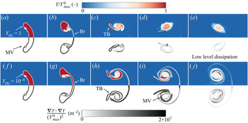
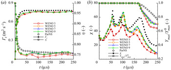
Figure 5 compares the temporal evolution of the helium mass fraction and scalar dissipation rate between VD and PS SBI. The general trend of scalar dissipation is increasing at the beginning and decreasing after the Br and TB structures are dissipated by vortex stretching into a steady-state of a‘well-mixed’ stage. From the normalised maximum helium concentration,  $\bar {Y}$ maintains a value of 1 during the stage of
 $\chi$ with high value, which means that the high scalar dissipation rate region is closely related to the maximum concentration. After the maximum concentration is stretched, the vortical mixing enters the diffusion controlling regime. Therefore, the most evident difference between VD and PS cases from the mixing indicators evolution is that the maximum concentration attains a steady state in the VD case much faster than that in the PS case. Thus, the SBI mixing time can be objectively defined when the maximum helium concentration decreases from one, and low-level dissipation is attained.
Normalised mass fraction (top) and scalar dissipation rate (bottom) for the  $Ma=2.4$ VD SBI case from (a) to (e). The
 $Ma=2.4$ PS SBI case is presented in the bottom line from (f) to (j). The moments captured are the same as those of figure 4.

3.3. Faster decay of VD mixing for different shock Mach numbers
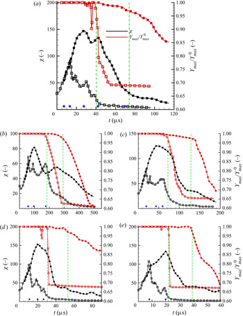
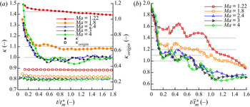
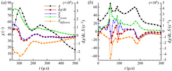
Figure 6(a) shows three stages of the mixing process separated from the profile of  $\chi$. Five blue circles in figure 6(a) indicate the five different moments in figures 4 and 5. For VD SBI, the first stage is the scalar dissipation growth owing to the vortex stretching before strong SBV occurs. After the Br is dissipated, the scalar dissipation rate enters the second stage, decreasing with time. Local peaks of scalar dissipation denote the stretching of TB structure by SBV during the decrease of dissipation, as shown in figure 4(c). Mixing enters the third stage at a late time, the steady diffusion stage, with a low value of
 $\chi$. This steady mixing state can be regarded as the final ‘well-mixed’ state, in which mixing no longer happens at a fast rate (Weber et al. Reference Weber, Haehn, Oakley, Rothamer and Bonazza2014).
Time history of scalar dissipation rate  $\chi$ (3.4) and maximum normalised mass fraction
 $\bar {Y}$ (3.5), for (a)
 $Ma=2.4$; (b)
 $Ma=1.22$; (c)
 $Ma=1.8$; (d)
 $Ma=3$; (e)
 $Ma=4$. For all figures, hollow points represent the VD case and solid points represent the PS case. Green dashed lines show the mixing time when
 $\bar {Y}=0.97$ is reached. Five blue circles in panel (a) indicate the five different moments in figures 4 and 5. Three blue circles presented separately in panels (b) to (e) indicate the three different moments for each Mach number in figure 30 of Appendix D.

For PS SBI, one can find a trend of the scalar dissipation  $\chi$ similar to that for the VD case from 7.2 to 13.2
 $\mathrm {\mu }$s, which means that the VD effect on mixing has not been illustrated. After the SBV at the Br structure is formed in the VD case at
 $13.2$
 $\mathrm {\mu }$s, the mixing behaviour of PS and VD SBI begins to diverge, which makes PS SBI mixing able to be maintained for a much longer time than VD SBI. Two
 $\chi$ peaks are observed during the increase of scalar dissipation in the PS case, which is different from the VD cases where
 $\chi$ peaks are related to SBV. The
 $\chi$ peaks in PS SBI are driven by strain from vorticity merging (VM), as indicated in figure 4(h). After the first
 $\chi$ peak, the bridge structure dissipates and VM from the TB structure contributes to the second
 $\chi$ peak, as shown in figure 6(a).
Figure 6(b–e) validate the similar growth trend in scalar dissipation  $\chi$ and normalised maximum concentration
 $\bar {Y}$ for different shock Mach numbers. For higher shock Mach number, mixing continues to require a shorter time for the VD SBI than for PS SBI owing to the higher compression and larger circulation. Interestingly, the differences between the PS and VD SBI for all Mach numbers start from the second stage, the dissipation decrease in the VD SBI, which leads to the shorter mixing time in the VD SBI than that in the PS SBI. The differences of
 $\chi$ peaks behaviour between the PS and VD SBI of other Mach numbers are further explained in Appendix D, which shows a similar mechanism with that of the
 $Ma=2.4$ case.
The maximum concentration  $\bar {Y}$ decrease faithfully tracks the beginning of the steady diffusion stage in both the VD SBI and PS SBI. It is noteworthy that some valley phenomena occur in the high Mach number VD cases. The appearance of a valley occurs a little earlier than the decay of the maximum concentration. We conjuncture that the valley results from the competition between density gradient accelerated dissipation and density gradient redistributed diffusion in VD flows (Yu, Liu & Liu Reference Yu, Liu and Liu2021). However, when a valley occurs, we observe that scalar dissipation is still at a relatively high value. Therefore, we denote the determinate decrease of maximum concentration as mixing time and the valley phenomena will be the focus of future study. Figure 6 shows the mixing time by dashed lines (VD SBI) and dash–dot lines (PS SBI) when
 $\bar {Y}=0.97$, as tabulated in table 3. Because the faster mixing is closely related to the scalar dissipation decrease in the VD SBI when the SBV of the Br structure forms, the SBV production mechanism and its effect on mixing are revealed in the next section.
Mixing time  $t_{\mathfrak {m}}$ of the VD and PS cases when
 $\bar {Y}=0.97$ is reached. Data are measured from figure 6.

4. Secondary baroclinic vorticity enhanced stretching mechanism
4.1. PS mixing mechanism: vortical stretching mixing
Because PS mixing does not influence vortical flow formation, the mixing is passively controlled by vortex stretching, as pointed out by Marble (Reference Marble1985) and Meunier & Villermaux (Reference Meunier and Villermaux2003). So the flow structure is essential for mixing. After the shock impact, the PS bubble obtains a translational velocity close to post-shock velocity  $u'_1$. If one sets the origin on the moving vortex centre (Shariff & Leonard Reference Shariff and Leonard1992), the azimuthal velocity around the vortex will be apparent as
 \begin{equation} V_{\theta}=\sqrt{(u-V_v)^2+v^2}, \end{equation}
in which  $u$ is the velocity in the
 $x$-direction and
 $v$ is the velocity in the
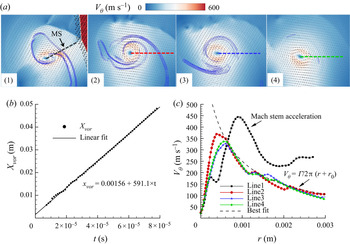
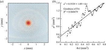
 $y$-direction. A more rigorous way to stand on the vortex centre (detailed definition of vortex centre position can be found in Appendix E) is to calculate the translational velocity of the vortex
 $V_v\approx 591.1$ m s
 $^{-1}$ that is plotted and linearly fitted in figure 7(b).
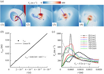
The PS SBI for  $Ma=2.4$. (a) Azimuthal velocity contour in the frame of the vortex centre at
 $t=13.2$
 $\mathrm {\mu }$s (a1),
 $t=27.6$
 $\mathrm {\mu }$s (a2),
 $t=42$
 $\mathrm {\mu }$s (a3) and
 $t=69.6$
 $\mathrm {\mu }$s (a4). Isoline of scalar dissipation rate is plotted as a blue line. (b) Motion of vortex centre with time. (c) Azimuthal velocity distribution along dashed lines in panels (a1)–(a4). Velocity distribution of a Lamb–Oseen-type vortex (4.2) is plotted as a dashed line, obtained from the best curve fit of descending data for Line 2.

Figure 7(a) shows the azimuthal velocity contour and vector defined by  $u-V_v$ and
 $v$. From the contour of the azimuthal velocity
 $V_{\theta }$, the velocity vector is mainly around the vortex centre. To quantify the velocity distribution, figure 7(c) gives the
 $V_{\theta }$ along defined lines of different moments, as illustrated in figure 7(a). From figure 7(a1), it can be observed that the Mach stem intrudes the vortex core, which is called ‘embedded shock’ first found in a compressible vortex ring (Dora et al. Reference Dora, Murugan, De and Das2014; Qin et al. Reference Qin, Xiang, Lin and Liu2020). Therefore, the defined Line 1 emerges in a high velocity region before encountering the Mach stem. Interestingly, after shock passage, the radial azimuthal velocity
 $V_{\theta }$ profiles of three later moments agree well with that of the spiral of a Lamb–Oseen vortex, which can be reduced to a point vortex model as
 \begin{equation} V_{\theta}\approx \frac{\varGamma}{2{\rm \pi}(r+r_0)}, \end{equation}
where  $\varGamma$ is the vortex circulation and
 $r_0=0.000439$ m is obtained from the best curve fit of descending data for Line 2. From the isolines of scalar dissipation, the scalar is stretched by the vortex passively until the diffusion stage. Thus, referring to Marble (Reference Marble1985) and Meunier & Villermaux (Reference Meunier and Villermaux2003), the PS SBI mixing time can be influenced by three main factors:
 \begin{equation} t_{\mathfrak{m}}^{PS}=f(\varGamma, \mathscr{D}, r), \end{equation}
where circulation  $\varGamma$ is a measure of stirring,
 $\mathscr {D}$ denotes diffusivity and
 $r$ is the distance between the passive scalar and vortex centre.
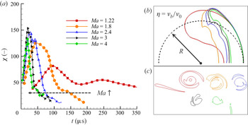
Here, we further check the shock compression effect on the PS SBI. As shown in figure 8(a), a higher Mach number leads to a shorter mixing time of scalar dissipation. It can be concluded that, except for the circulation deposited by shock impact, the area that needs to be stirred is also essential for determining when mixing becomes stable. As shown in figure 3(b), the compression rate  $\eta$ for both the PS and VD cases maintains a lower value at higher shock Mach number. In the VD SBI, the compression rate was proposed and theoretically modelled by Giordano & Burtschell (Reference Giordano and Burtschell2006) and studied by Niederhaus et al. (Reference Niederhaus, Greenough, Oakley, Ranjan, Anderson and Bonazza2008). Recently, a quantitative scaling of the final mixing extent proportional to the compression rate was built by Yu et al. (Reference Yu, Liu and Liu2021). Because the PS bubble's compression rate is nearly the same as that of the VD bubble's, the compression effect by shock impact is believed to be another factor for the shorter mixing time at a higher shock Mach number. A more intuitive explanation is the different helium areas for different shock Mach numbers in figures 8(b) and 8(c). The initial conditions for the PS SBI show that the area for mixing shrinks to
 $\mathcal {V}_b=\eta \mathcal {V}_0$ (2.17), where
 $\mathcal {V}_0$ is the initial un-shocked cylindrical bubble volume. A higher Mach number leads to smaller compression rate and PS bubble area, as indicated in figure 8(b). Here, a general form of the PS SBI mixing time can be stated as
 \begin{equation} t_{\mathfrak{m}}^{PS}=f(\varGamma, \mathscr{D}, r, \eta). \end{equation}
(a) Time history of scalar dissipation rate for PS SBI with different shock Mach number. (b) Isoline of cylindrical bubble boundary at initial time to show the compression effect on initial mixing region  $\mathcal {V}_b=\eta \mathcal {V}_0\approx \eta {\rm \pi}R^2$ and (c) final mixing region of PS SBI for different shock Mach number. Red,
 $Ma=1.22$; orange,
 $Ma=1.8$; blue,
 $Ma=2.4$; black,
 $Ma=3$; green,
 $Ma=4$.

4.2. VD mixing mechanism: additional SBV-enhanced stretching
To render the mechanism causing faster mixing decay in the VD SBI, we apply the same data treatment to the VD case, as shown in figure 9. The vortex of the VD cases translates at nearly the same velocity as in the PS case at  $V_v\approx 605.7$ m s
 $^{-1}$, as shown in figure 9(b). Under the coordinate of the vortex centre, the azimuthal velocity contours of the VD case at four different moments are illustrated in figure 9(a), where the legend is the same as that for the PS case. The obvious difference is focused on the much greater azimuthal velocity
 $V_{\theta }$ at the bridge structure and the region around the vortex. In figure 9(c), this velocity increase is clearly shown by the velocity profile along the defined lines of figure 9(a). The lines are characterised as one end originates from the vortex centre pointing to the location of maximum azimuthal velocity. For comparison, the PS SBI velocity profiles along the defined lines in figure 7(c) are also shown. The increased velocity at the bridge structure (VD Line 1) is shown to be more than twice the velocity in PS SBI. At a distance far from the acceleration region, where the bubble concentration is low, the azimuthal velocity returns to the Lamb–Oseen vortex model, as displayed in (4.2). Thus, it can be inferred that this velocity increase is caused by the SBV, denoted by
 $\Delta V_{\theta }^b$,
 \begin{equation} \tilde{V}_{\theta}\equiv V_{\theta}+\Delta V_{\theta}^{b}, \end{equation}
where  $\tilde {V}_{\theta }$ refers to the azimuthal velocity distribution in the VD SBI. Furthermore, the increase in stretching velocity
 $\Delta V_{\theta }^b$ can be directly related to the local production of SBV
 $\omega _b$. One can easily derive the relation between local vorticity and its azimuthal velocity distribution:
 \begin{equation} \frac{\partial \tilde{V}_{\theta}}{\partial r}=\frac{\partial V_\theta}{\partial r}+\frac{\partial \Delta V_{\theta}^{b}}{\partial r}\equiv\omega_{pv}+\omega_{b}= \omega, \end{equation}
where  $\omega _{pv}$ is the vorticity attributed to a point vortex part,
 $\omega _b$ is the local SBV part and
 $\omega$ is the total vorticity magnitude along the radius locally. From the isolines of scalar dissipation in figure 9(a), the azimuthal velocity increase stretches the bubble structure and enhances the mixing rate. That explains the faster mixing in the VD SBI than in the PS SBI and reveals the intrinsic VD effect: the lighter gas responds faster than the heavy gas through local SBV production, which implies an asymmetric mixing behaviour in VD flows.
VD SBI for  $Ma=2.4$. (a) Azimuthal velocity contour in the frame of the vortex centre at
 $t=13.2$
 $\mathrm {\mu }$s (a1),
 $t=27.6$
 $\mathrm {\mu }$s (a2),
 $t=42$
 $\mathrm {\mu }$s (a3) and
 $t=69.6$
 $\mathrm {\mu }$s (a4). (b) Motion of the vortex centre with time. (c) Azimuthal velocity distribution along the defined lines captured from panels (a1) to (a4) compared with azimuthal velocity distribution at the same time obtained from figure 7. An increase of azimuthal velocity in the VD case is obvious for each comparison.

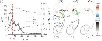
To determine the origin of the increase in velocity arising from SBV, one should check the vorticity generation mechanism. It has been proven that after the shock interaction, the main circulation is conserved inside the mixing region confined by the mass fraction contour, as shown in § 2. The conservation of circulation indicates that the same quantitative positive vorticity is produced to balance the negative vorticity from SBV. Here the total circulation, normalised by the final equilibrium circulation, is decomposed into the positive and negative ones,
 \begin{equation} \varGamma_t/\varGamma=\varGamma^+{/}\varGamma+\varGamma^-{/}\varGamma, \end{equation}
as validated in figure 10(a), which shows the same up and down characteristic of opposite sign circulation.
(a) Synchronous growth of opposite sign vorticity and scalar dissipation for  $Ma=2.4$ VD SBI. (b) Isolines of vorticity (top) and contour of scalar dissipation (bottom) at instants near
 $t_{b}=13.2$
 $\mathrm {\mu }$s: (b1)
 $11.2$
 $\mathrm {\mu }$s; (b2)
 $13.2$
 $\mathrm {\mu }$s; (b3)
 $15.2$
 $\mathrm {\mu }$s.

The SBV production process in the VD SBI is illustrated in figure 10(b). The main vortex will come near the bubble's interface where the density gradient at the bridge structure exists. The roll-up process of the vortex will accelerate the interface leading to the acceleration  $\mathrm {d}({V}_{\theta }\boldsymbol {e}_{\boldsymbol {\theta }})/\mathrm {d}t$ in the azimuthal direction
 $\boldsymbol {e}_{\boldsymbol {\theta }}$ (Peng et al. Reference Peng, Zabusky and Zhang2003). Assuming negligible gravitational force and incompressible flow, one obtains
 $\mathrm {d}({V}_{\theta }\boldsymbol {e}_{\boldsymbol {\theta }})/\mathrm {d}t=-1/\rho \boldsymbol {\nabla } p$ (Reinaud, Joly & Chassaing Reference Reinaud, Joly and Chassaing2000). Owing to the existence of the density gradient
 $\boldsymbol {\nabla }\rho$, the baroclinic vorticity production will follow
 \begin{equation} \frac{\mathrm{D}\boldsymbol{\omega}_{\boldsymbol{b}}}{\mathrm{D}t}=\frac{1}{\rho^2}\boldsymbol{\nabla}\rho\times\boldsymbol{\nabla} p=\frac{1}{\rho} \frac{\mathrm{d}({V}_{\theta}\boldsymbol{e}_{\boldsymbol{\theta}})}{\mathrm{d}t}\times\boldsymbol{\nabla}\rho. \end{equation}
From this equation, we can find that mixing will smear the density gradient  $\boldsymbol {\nabla }\rho$ and thus decrease the SBV production. SBV will provide feedback on the mixing rate through the local stretching.
The integral effect of SBV on scalar dissipation is recorded in figure 10(a). The time history of the scalar dissipation rate is closely related to the SBV circulation profile, which shows that the stretching from SBV controls the mixing rate. The watershed of the increase and decrease of scalar dissipation is at the moment  $t=t_{b}$, when the SBV peak is attained, as shown in figure 10(a). From figure 10(b2), it can also be found that when SBV forms near the bridge structure, the local scalar dissipation becomes strong. In figure 10(b3), after the production of SBV, the local baroclinic vorticity begins to decrease because mixing smears the density gradient
 $\boldsymbol {\nabla }\rho$ and reduces the production of SBV, as analysed.
It is noteworthy that the intense mixing rate at the bridge structure is also found in shock–heavy cylinder interactions (Tomkins et al. Reference Tomkins, Kumar, Orlicz and Prestridge2008). The non-turbulent band of a fluid is the most high-level mixing region. It is concluded that the vortex stretching effect at the bridge contributes 40 % of the mixing rate over all time. Tomkins et al. (Reference Tomkins, Kumar, Orlicz and Prestridge2008) explained this high mixing rate as the strong strain rate. In this study, the bridge structure's dissipation in the shock–light bubble interaction is further revealed as the additional stretching from the SBV. As soon as the SBV occurs, the fast stretching of the bridge structure makes the density gradient across the Br structure decrease, not like in the shock–heavy bubble interaction where the bridge structure can sustain mixing.
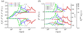
Moreover, checking the normalised SBV circulation growth for different shock strength, one can find that the same magnitude of positive and negative vorticity occurs in all cases concerned, as shown in figure 11(a). Because positive circulation contains the initial shock-induced vorticity, the absolute value of negative circulation,  $|\varGamma ^-/\varGamma |$ solely attributed to negative SBV vorticity, can be denoted as SBV circulation. Similar to the
 $Ma=2.4$ case, the synchronous growth of SBV circulation and scalar dissipation rate in other shock Mach number cases is also confirmed in figure 11(b). The SBV circulation peak value is higher as shock strength increases and happens at the time of bridge structure formation. We further record the temporal evolution of maximum azimuthal velocity
 $V_\theta ^{max}$ for each VD case in figure 11(b). It can be found that when the SBV circulation peak is reached, the peak value of azimuthal velocity occurs, in accordance to the azimuthal velocity profiles in figure 9(c). The relation between SBV peak and azimuthal velocity peak value will be discussed and modelled in § 4.3.
(a) Dimensionless positive, negative and total circulation in different Mach number cases. (b) The synchronous growth of scalar dissipation and the secondary baroclinic circulation in different Mach number cases. The maximum azimuthal velocity  $V_\theta ^{max}$ normalised by post-shock velocity
 $u_1'$ is also plotted.

4.3. Velocity difference model for azimuthal acceleration from SBV
4.3.1. SBV model:  $\omega _b$

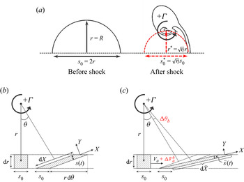
Figure 12 shows the illustration of the formation of the bridge structure and the SBV. Because the cylindrical bubble is lighter than ambient air, the upstream edge's velocity  $u'_2$ is much larger than that of the downstream edge, the same as the shocked air
 $u'_1$ (Yu et al. Reference Yu, He, Zhang and Liu2020). A vortex is first formed in the upstream edge and moves at approximately
 $u'_2$ at the beginning. Then we can simplify this process as a model problem as illustrated in the magnified frame in figure 12. In the coordinate of the vortex core, the bridge structure containing a density interface moves towards the vortex with circulation
 $\varGamma$ at a speed of
 $\Delta U=u'_2-u'_1$. The deposited SBV accumulates as the density interface moves. As discussed in PS SBI, the velocity profile in the mixing region can be fitted by a point vortex before the SBV occurs. Thus, it is appropriate to use the assumption that the
 $V_{\theta }$ is reciprocal to the distance to the main vortex core
 $r$:
 \begin{equation} V_{\theta}=\frac{\varGamma}{2{\rm \pi} r}. \end{equation}
Thus, the acceleration of the bridge interface can be illustrated as
 \begin{equation} \frac{\mathrm{d}V_{\theta}}{\mathrm{d}t}=\frac{\mathrm{d}V_{\theta}}{\mathrm{d}r} \frac{\mathrm{d}r}{\mathrm{d}t} =\frac{\varGamma\Delta U}{2{\rm \pi} r^2}, \end{equation}
because the density interface is approaching the main vortex core at the speed  $\Delta U$, which is
 ${\mathrm {d}r}/{\mathrm {d}t}=-\Delta U$. The density gradient
 $\boldsymbol {\nabla }\rho$ in (4.8) is presumed to be perpendicular to the azimuthal acceleration
 $\mathrm {d}({V}_{\theta }\boldsymbol {e}_{\boldsymbol {\theta }})/\mathrm {d}t$ and directed along the
 $r$-axis (it has no component in any other direction). Then the magnitude of the density gradient
 $|\boldsymbol {\nabla }\rho |=\mathrm {d}\rho /\mathrm {d}r$, and the local secondary baroclinic vorticity production rate can be expressed as
 \begin{equation} \dot{\omega}_{b}=\frac{\mathrm{D}\omega_{b}}{\mathrm{D}t}=\frac{1}{\rho}\frac{ \mathrm{d}V_\theta }{\mathrm{d}t} \frac{\mathrm{d}\rho}{\mathrm{d}r}. \end{equation}
Illustration of the SBV production at the bridge structure by a velocity difference model abstracted from the shocked light gas cylindrical bubble and shocked heavy ambient air.

From figure 12, we can make several assumptions about  $\mathrm {d}\rho /\mathrm {d}r$:
(i) inside the density interface, the density is invariant with time, which is a light gas density
$\rho _2'$ inside the density interface and a heavy gas density $\rho _1'$ outside the density interface;(ii) the density interface is compact and symmetrical about
$r(t)$;(iii) the thickness of the density interface transition layer
$\delta '$ at the post-shock bridge structure is equal to $\sqrt {\eta }\delta$, where $\delta$ is the initial transition layer introduced in § 2.2 (see Appendix F for details);(iv) the thickness
$\delta '$ is much smaller than $r$, i.e. $\delta '=O(\mathrm {d}r)$.


These four assumptions are made to describe the bridge structure formation. Therefore,  $\mathrm {d}\rho /\mathrm {d}r$ can be expressed as
 \begin{equation} \frac{\mathrm{d}\rho}{\mathrm{d}r}\approx\left\{ \begin{array}{@{}ll} 0 & r\in(0,r(t)-\delta'), \\ \dfrac{\rho_1'-\rho_2'}{\delta'} & r\in[r(t)-\delta',r(t)), \\ 0 & r=r(t), \\ \dfrac{\rho_2'-\rho_1'}{\delta'} & r\in(r(t),r(t)+\delta'], \\ 0 & r\in(r(t)+\delta',+\infty). \end{array}\right. \end{equation}
For convenience, we only consider the value at point  $r(t)$, which is related to the range
 $[r(t)-\delta ',r(t))$ at the upwind side of the density interface transition layer. Then the baroclinic vorticity production rate in this range can be further calculated as
 \begin{equation} \dot{\omega}_{b}=\frac{1}{\rho}\frac{\varGamma\Delta U}{2{\rm \pi} r^2}\left(\frac{\mathrm{d}\rho}{\mathrm{d}r}\right) \approx\frac{\varGamma\Delta U|{At}^+|}{{\rm \pi}\delta' r^2}, \quad r\in[r(t)-\delta',r(t)), \end{equation}
where  $\rho$ can be the average density
 $(\rho _1'+\rho _2')/2$ and
 $r$ is the distance from the vortex core, as shown in figure 12. Then, the baroclinic vorticity production can be calculated as
 \begin{equation} \omega_b(r,t+\mathrm{d}t)=\omega_b(r,t)+\dot{\omega}_{b}\,\mathrm{d}t\Rightarrow \omega_{b}=\int_0^{t}\dot{\omega}_{b}\,\mathrm{d}t'. \end{equation}
To complete the set of equations, the distance between the bridge and the main vortex  $r$ in (4.13) should be modelled. In figure 12, one can find that
 $r$ is the function of time:
 \begin{equation} r(t)\approx D-\Delta{U}t. \end{equation}
Hence, the baroclinic vorticity growth (4.14) can be expressed as
 \begin{align} \omega_{b} & = \int_0^{t}\frac{\varGamma\Delta U|{At}^+|}{{\rm \pi}\delta' r^2} \,\mathrm{d}t' =\frac{\varGamma\Delta U|{At}^+|}{{\rm \pi}\delta'} \int_0^{t} \frac{1}{(D-\Delta Ut')^2}\,\mathrm{d}t' \nonumber\\ & = \left.\frac{\varGamma|{At}^+|}{{\rm \pi}\delta'}\frac{1}{D-\Delta Ut'} \right|_{0}^{t} = \frac{\varGamma|{At}^+|}{{\rm \pi}\delta'}\left(\frac{1}{D-\Delta Ut}-\frac{1}{D}\right) \nonumber\\ & = \frac{\varGamma|{At}^+|}{{\rm \pi}\delta'}\left(\frac{1}{r}-\frac{1}{D}\right), \quad r\in[r(t)-\delta',r(t)). \end{align}
Using  $D^2$ as the characteristic area, the normalised baroclinic vorticity at
 $t=t_b$, where
 $t_{b}$ is the time of the bridge formation and is also the first time of the synchronous growth of the opposite sign circulation peak in figure 11(b), can be obtained:
 \begin{equation} \frac{\omega_{b}D^2}{\varGamma}=\frac{|{At}^+|D}{{\rm \pi}\delta'}\left(\frac{1}{1-\Delta Ut_b/D}-1\right). \end{equation}
The SBV model (4.17) predicts the normalised baroclinic vorticity at the bridge structure, which should be proportional to the peak value of SBV circulation  $|\varGamma ^-/\varGamma |$ (denoted as
 $\varGamma _{b}/{\varGamma }$ hereafter) in figure 11(b). To validate (4.17), we first provide evidence of the proportionality between
 $\varGamma _b$ and
 $\omega _b D^2$ from the measured data and then compare with the SBV model.
The vorticity contours at  $t=t_b$ for each Mach number are plotted in figure 13(a) (
 $Ma=2.4$ can be found in figure 10b2). A defined line is extracted from the vorticity contour to illustrate the vorticity distribution along the axis
 $r$ with the origin at the vortex core. Axis
 $r$ points to the location of maximum azimuthal velocity
 $V_\theta ^{max}$. The distributions of vorticity along the axis
 $r$ for different cases are plotted in figure 13(b). The crest and trough are observed, meaning the SBV layer. Because positive vorticity can not eliminate the shock-induced initial vorticity deposition from SBV (same reason as SBV circulation), we measure the peak negative vorticity
 $\omega _{b,p}$ for each case, as indicated in figure 13(b).
(a) Vorticity contour for different Mach number VD SBI cases at  $t=t_b$, namely,
 $Ma=1.22$,
 $t_b=58$
 $\mathrm {\mu }$s;
 $Ma=1.8$,
 $t_b=19.2$
 $\mathrm {\mu }$s;
 $Ma=3$,
 $t_b=11$
 $\mathrm {\mu }$s;
 $Ma=4$,
 $t_b=8$
 $\mathrm {\mu }$s. Coordinate
 $r$ with origin at the vortex centre pointing to the location of maximum azimuthal velocity
 $V_\theta ^{max}$ is built for each case. (b) Vorticity profile along axis
 $r$ built in panel (a) for each case. Profile for the
 $Ma=2.4$ case is extracted as the data from VD Line 1 in figure 9(c) and vorticity contour in figure 10(b2). (c) SBV circulation
 $|\varGamma ^-/\varGamma |$ for different shock Mach numbers versus the scaled time
 $\Delta Ut/D$.

As for the peak value of SBV circulation  $|\varGamma ^-/\varGamma |$, the baroclinic circulation under the scaling of
 $\Delta Ut_b/D$ is shown in figure 13(c). From 1-D gas dynamics, we can theoretically obtain the velocity difference
 $\Delta {U}$ between the shocked bubble upstream interface
 $u'_2$ and the ambient air
 $u'_1$. The direct link between the velocity difference
 $\Delta {U}$ and
 $t_{b}$ can be found:
 \begin{equation} \frac{\Delta{U}t_{b}}{D}=0.54\sim0.68 \quad \textrm{for } Ma=1.22\sim 4. \end{equation}
At approximately  $\Delta Ut/D\approx 0.6$, the peak of baroclinic circulation is obtained and is tabulated in table 4. From the last column of the table, the proportional relation between
 $\varGamma _b$ and
 $\omega _{b,p}D^2$ is evident. Moreover, through the value of
 $t_b$, the SBV model (4.17) can be validated:
 \begin{equation} \frac{\omega_bD^2}{\varGamma}\propto\frac{\varGamma_b}{\varGamma}\propto\frac{\omega_{b,p}D^2}{\varGamma}. \end{equation}
The evidence of the proportionality between  $\varGamma _b$ and
 $\omega _bD^2$ is the (near) constancy of the parameter
 $k$ in table 4, which shows that the simplified model, as illustrated in figure 12, is appropriate.
One-dimensional gas dynamics is used to provide  $\Delta {U}=u'_2-u'_1$. Here,
 $t_{b}$ is the time at the first maximum of baroclinic circulation growth referring to figure 12;
 $k\equiv (\omega _bD^2)/\varGamma _b$, where
 $\omega _b$ is obtained from (4.17) at
 $t=t_b$;
 $\varGamma _b/\varGamma$ is the peak value of
 $|\varGamma ^-/\varGamma |$ from figure 13(c); and
 $\omega _{b,p}$ is the peak negative vorticity measured from figure 13(b).

4.3.2. Azimuthal velocity increase model: $\Delta V_{\theta }^b$

In this part, the azimuthal velocity increased by SBV is modelled and validated. We have noted the derivative relation between baroclinic increased azimuthal velocity and SBV (4.6):
 \begin{equation} \omega_b=\frac{\partial \Delta V_{\theta}^b}{\partial r}. \end{equation}
Integrating SBV in (4.16) from the origin to radius  $r(t)$, we obtain
 \begin{equation} \Delta V_{\theta}^b = \int_0^{r(t)} \omega_b \,\mathrm{d}r =\frac{\varGamma|{At}^+|}{{\rm \pi}\delta'}\int_0^{r(t)} \left(\frac{1}{r}-\frac{1}{D}\right)\mathrm{d}r. \end{equation}
Owing to the fact that SBV at  $(0,r(t)-\delta ')$ is zero (density gradient is zero and see figure 12), the SBV-induced azimuthal velocity increase at
 $r(t_b)$ is
 \begin{align} \Delta V_{\theta}^b & =\frac{\varGamma|{At}^+|}{{\rm \pi}\delta'}\int_{r(t_b)-\delta'}^{r(t_b)} \left(\frac{1}{r}-\frac{1}{D}\right)\mathrm{d}r\nonumber\\ & =\frac{\varGamma|{At}^+|}{{\rm \pi}\delta'}\left[\ln \left(\frac{r(t_b)}{r(t_b)-\delta'}\right)-\frac{\delta'}{D}\right] \nonumber\\ & = \frac{\varGamma|{At}^+|}{{\rm \pi}\delta'}\left[\ln \left(\frac{D-\Delta Ut_b}{D-\Delta Ut_b-\delta'}\right)-\frac{\delta'}{D}\right]. \end{align}
Therefore, from (4.5), the total azimuthal velocity at  $t=t_b$, when peak azimuthal velocity is reached, is composed of the point vortex induced part
 $V_{\theta }$ and SBV-induced part
 $\Delta V_{\theta }^b$:
 \begin{equation} \tilde{V}_{\theta}=V_{\theta}+\Delta V_{\theta}^b=\frac{\varGamma}{2{\rm \pi} r_m}+ \frac{\varGamma|{At}^+|}{{\rm \pi}\delta'}\left[\ln \left(\frac{D-\Delta Ut_b}{D-\Delta Ut_b-\delta'}\right)-\frac{\delta'}{D}\right], \end{equation}
where  $r_m$ is the distance from the vortex centre.
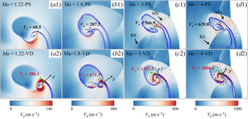
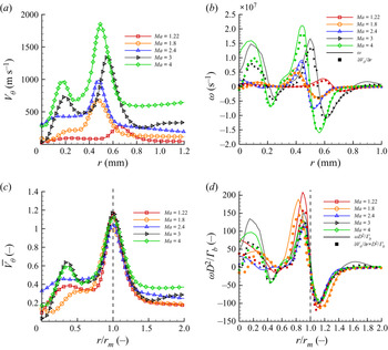
Figure 14 shows the azimuthal velocity contour for different shock Mach numbers for both PS SBI and VD SBI (the velocity of vortex  $V_v$ is studied in Appendix E). A higher azimuthal velocity for the VD cases is shown for all Mach numbers, which explains the faster mixing for the VD cases than PS cases. To quantify the azimuthal velocity distribution of the VD SBI, the same coordinate
 $r$ as that in figure 13(a) is examined, as shown in figure 15(a). The location
 $r_m$ and the value of the maximum azimuthal velocity can be obtained, which should agree with the maximum azimuthal velocity recorded in figure 11(b). Interestingly, the derivative of the azimuthal velocity along axis
 $r$ is near the local vorticity distribution, as shown in figure 15(b), which validates the relation between SBV and its induced velocity increase (4.6). Moreover, it can be inferred that the vorticity attributed to the point vortex model is much smaller than SBV, which satisfies the zero vorticity of the standard point vortex model (Wu, Ma & Zhou Reference Wu, Ma and Zhou2007). The high vorticity near the vortex core for high Mach numbers arises from the entrainment of vorticity from the bottom of the vortex centre. The azimuthal velocity distribution normalised by the modelled value (4.23),
 $\bar {V}_\theta$, is presented in figure 15(c). Good agreement can be observed when
 $r=r_m$,
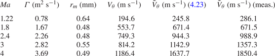
 $\overline {V}_\theta \approx 1$. The general trend of the modelled value is consistent with the measured value, as tabulated in the last two columns of table 5.
Azimuthal velocity distribution in the frame of a vortex centre for different shock Mach numbers for VD SBI [shown as panels (a2) to (d2)] by comparing with results for PS SBI [shown as panels (a1) to (d1)]. The moments captured and coordinate  $r$ are the same as those in figure 13(a).

(a) Azimuthal velocity distribution along the axis  $r$ in figure 14 for VD SBI with different shock Mach numbers. (b) The comparison between
 $\partial \tilde {V}_{\theta }/\partial r$ and vorticity distribution along the axis
 $r$ in figure 13(b). (c) Azimuthal velocity normalised by the modelled value (4.23) along the normalised axis
 $r/r_m$. (d) Normalised vorticity
 $\omega D^2/\varGamma _b$ along the normalised axis
 $r/r_m$.


In summary, §§ 4.2 and 4.3 reveal the additional stretching of SBV in the VD cases, which explains the shorter mixing time in the VD SBI. Because the vortex stirring, compression effect and diffusion in the PS SBI are shared in the VD cases, the mixing time for the VD SBI can be implicitly expressed by adding the baroclinic azimuthal velocity increase  $\Delta V_{\theta }^b$:
 \begin{equation} t_{\mathfrak{m}}^{VD}=f[\varGamma,\mathscr{D},r,\eta,\Delta V_{\theta}^b(\omega_b)]. \end{equation}
Section 5 will discuss the mixing time for the PS SBI and VD SBI based on the reduced-order model of baroclinic vorticity dynamics.
5. A novel mixing time for VD SBI
Based on the mixing mechanism for the PS SBI revealed in (4.4) and for the VD SBI revealed in (4.24), stirring, diffusion, compression from shock and the density effect are systematically considered for modelling mixing behaviour within a vortical flow.
5.1. Characteristic mixing time for PS SBI
From § 4.1, it is observed that the mixing of the PS SBI follows a typical vortical stretching enhanced mixing. For the vortical flow stretching velocity  $V_{\theta }$, Meunier & Villermaux (Reference Meunier and Villermaux2003) theoretically proposed a characteristic mixing time for a PS blob with length
 $s_0$, at distance
 $r$ away from vortex centre stretched by vortical flows, as illustrated in figure 16(b):
 \begin{equation} t_{\mathfrak{m}}^{PS}=t_{m}=f(\varGamma, \mathscr{D}, r)=\frac{r^2}{\varGamma}\left(\frac{3{\rm \pi}^2}{16}\right)^{1/3}\left(\frac{s_0}{r}\right)^{2/3} \left(\frac{\varGamma}{\mathscr{D}}\right)^{1/3}. \end{equation}
When  $t/t_m>1$, the maximum concentration will be below the initial concentration, i.e.
 $\bar {Y}<1$, and mixing enters the diffusion-controlled stage. Here,
 $t_m$ displays the Péclet number
 $Pe=\varGamma /\mathscr {D}$ dependence. A similar
 $Pe^{1/3}$ dependency was also derived for a flame vortex interaction modelled by Marble (Reference Marble1985) and was used to evaluate the mixing time in a supersonic streamwise vortex by Waitz et al. (Reference Waitz1997). To agree with the physical characteristic of (5.1), let
 $r=R$ be the cylindrical bubble radius and
 $s_0=2r$, as shown in figure 16(a).
(a) Compression effect on initial mixing region; (b) stretching of PS blob under the standard point vortex (Meunier & Villermaux Reference Meunier and Villermaux2003); (c) SBV-enhanced stretching in VD mixing.

Figure 17 shows the time history of normalised maximum concentration,  $\bar {Y}$, and scalar dissipation,
 $\chi$, under the dimensionless scaling of
 $t/t_m$. For
 $Ma=1.22$, at
 $t/t_m\approx 1$, the maximum concentration decrease agrees well with the theoretical prediction. A similar trend is found in the scalar dissipation
 $\chi$ as most of the mixing rate is high before
 $t/t_m<1$ for the PS SBI at
 $Ma=1.22$. This agreement shows that the scaling by (5.1) is appropriate for the general vortical mixing flows, such as the PS SBI. However, it is found that it can not scale the mixing of the PS SBI for all Mach numbers, especially the cases of high Mach number. The agreement for
 $Ma=1.22$ can be explained by the fact that shock compression effects on mixing are relatively weak in this scenario. Thus, a definition of mixing time considering shock compression effects is needed.
(a) Maximum concentration decay and (b) scalar dissipation for PS SBI versus scaled time  $t/t_{m}$, where
 $t_m$ is expressed in (5.1).

From § 4.1, it is further found that after the initial shock, the cylindrical bubble is compressed and shrinks volumetrically, as depicted in figure 8(b). In other words, the amount of scalar left to be stirred by the vortex is reduced by a rate  $\eta$ compared with the initial bubble volume (2.17). This finding can be stimulated to revise the characteristic length
 $s_0$ and distance from the vortex centre
 $r$:
 \begin{equation} \mathcal{V}_b=\frac{{\rm \pi} r^* s_0^*}{2}=\eta \frac{{\rm \pi} r s_0}{2}=\eta \mathcal{V}_0 \Rightarrow \quad r^*=\sqrt{\eta}r \text{ and } s_0^*=\sqrt{\eta}s_0. \end{equation}
As illustrated in the right part of figure 16(a), (5.2) denotes a compressed cylindrical bubble, with radius  $r^*$ and centreline diameter
 $s_0^*$, stirred by a point vortex located at the bubble top. This physical process can reflect the PS SBI mixing to some extent as discussed in Appendix G. After revising
 $s_0^*$ and
 $r^*$ in (5.1), the mixing time for passive scalar that considers compression can be expressed as
 \begin{equation} t_{\mathfrak{m}}^{PS}=t_{m}^*=f(\varGamma, \mathscr{D}, r, \eta)=\frac{\eta r^2}{\varGamma}\left(\frac{3{\rm \pi}^2}{16}\right)^{1/3}\left(\frac{\sqrt{\eta}s_0}{\sqrt{\eta}r}\right)^{2/3} \left(\frac{\varGamma}{\mathscr{D}}\right)^{1/3}. \end{equation}
It reveals the proportional relationship between the scalar mixing time and the compression rate. Figure 18 shows the  $\bar {Y}$ and
 $\chi$ versus the scaled time
 $t/t_m^*$, which scales all shock Mach number cases well. At
 $t/t_m^*>1$, the maximum concentration begins to decrease and the mixing rate tends to a low level of diffusion-controlled mixing, which validates that for vortical stretching, a compression effect by the initial shock impact is vital for the time that mixing can sustain.
(a) Maximum concentration decay and (b) scalar dissipation for PS SBI versus scaled time  $t/t^*_{m}$. By considering compression effects from the shock on the initial mixing region, the mixing time can be correctly predicted at a time scale of
 $t/t^*_{m}\approx 1$, where
 $t^*_m$ is expressed in (5.3).

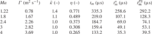
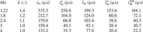
Table 6 gives intuitive values that are required for calculating  $t_m$ and
 $t_m^*$. For all Mach numbers,
 $t_m$ overestimates the mixing time for the PS SBI, as discussed. Interestingly, although
 $t_m^*$ is much nearer to the measured values, it always underestimates the mixing time, especially for low Mach number. The inferred reason is that the PS SBI cases set in this paper are not standard point vortex models. It takes some time before the PS SBI forms into a quasi-standard point vortex model; that explains the extra time in the measured values compared with those theoretically modelled. A comparison between scalar mixing under a standard Lamb–Oseen vortex and
 $Ma=1.22$ PS SBI confirm the deduction, as discussed in Appendix G.
Comparison between theoretical mixing time from (5.1), (5.3) and measured value referring to table 3. The circulation  $\varGamma$, diffusivity coefficient
 $\bar {\kappa }$ (see Appendix C) and compression rate
 $\eta$ are also listed.

5.2. Characteristic mixing time for VD SBI
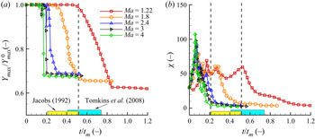
Figure 19 shows the time history of two mixing indicators versus the dimensionless timescale by the canonical mixing time (5.1). In the previous research of the SBI, Jacobs (Reference Jacobs1992) first introduced this mixing time in the shock–light cylindrical bubble interaction, which is close to the case studied in the VD SBI with  $Ma=1.22$. It was concluded that mixing occurs in the range of
 $0.10< t/t_m<0.25$ by setting
 $r=D$ and
 $t_m=r^2/(\varGamma ^{2/3}\mathscr {D}^{1/3})$, only with a different coefficient
 $2^{-4/3}(3{\rm \pi} ^2/16)^{1/3} \approx 0.487$ compared to (5.1). Thus, we convert the mixing sustaining time from Jacobs (Reference Jacobs1992) to
 $0.205< t/t_m<0.51$. Interestingly, the mixing time revealed by Jacobs (Reference Jacobs1992) coincides with the case in this work, as presented in figure 19(a). When
 $t/t_m>0.51$, the normalised maximum concentration
 $\bar {Y}$ begins to decrease. Moreover, a high mixing rate is found during the sustaining mixing period, as shown in figure 19(b). Further study on a shock–heavy cylindrical bubble interaction by Tomkins et al. (Reference Tomkins, Kumar, Orlicz and Prestridge2008) showed similar results with mixing occurring at
 $0.41< t/t_m<0.74$, although the overlap region is relatively weak. In short summary, (5.1) still largely overestimates the mixing time in the VD SBI in general.
(a) Maximum concentration decay and (b) scalar dissipation for the VD SBI versus scaled time  $t/t_{m}$. Under the scaling of mixing time
 $t_{m}$ (5.1), the VD SBI cases show large discrepancy for different shock Mach number cases.

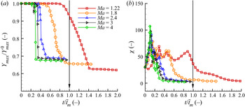
It has been observed that SBV-induced additional stretching occurs in the VD SBI, compared with the PS SBI. The additional stretching is not considered in a single point vortex velocity distribution, as modelled in (5.1). In § 4.3, we have built the SBV-increased azimuthal velocity model  $\tilde {V}_{\theta }$ for the VD SBI. Here, we combine this model with the advection–diffusion equation to quantify the effect of additional stretching on the mixing time. Starting from the azimuthal velocity
 $\tilde {V}_{\theta }$ of the VD SBI, referring back to figure 12, the shocked light bubble moves faster than the shocked ambient air with a velocity increase
 $\Delta U$. This SBV-accelerated stretching leads to an intuitive model, as shown in figure 16(c). Thus from (4.5), the azimuthal velocity can be expressed as
 \begin{equation} \tilde{V}_{\theta}=\frac{\varGamma}{2{\rm \pi} r}+\Delta{V}^b_{\theta}. \end{equation}
Noting that the azimuthal velocity from a point vortex is steady with time, the acceleration is mainly attributed to SBV-enhanced stretching. Here, we can obtain an abbreviation for SBV-enhanced stretching  $\Delta V_{\theta }^b$ from (4.22):
 \begin{align} \Delta{V}^b_{\theta} & = \frac{\varGamma|{At}^+|}{{\rm \pi}\delta'}\left[\ln \left(1+\frac{\delta'}{r-\delta'}\right)-\frac{\delta'}{D}\right] \nonumber\\ & \approx \frac{\varGamma|{At}^+|}{\rm \pi}\left(\frac{1}{r}-\frac{1}{D}\right), \end{align}
by noting that  $\delta '=O(\mathrm {d}r)$ and
 $r=O(R)$, which means
 $\delta '\ll r$,
 $\ln (1+\delta '/(r-\delta '))\approx \delta '/r$. Thus, the azimuthal velocity can be further expressed as
 \begin{equation} \tilde{V}_{\theta}=\frac{\varGamma}{2{\rm \pi} r}(1+2|{At}^+|)-\frac{\varGamma|{At}^+|}{{\rm \pi} D}. \end{equation}
As shown in figure 16(c), a blob is stretched under this velocity  $\tilde {V}_{\theta }$. The turning angle
 $\tilde {\theta }$ of this bubble at distance
 $r$ from the vortex centre is (Meunier & Villermaux Reference Meunier and Villermaux2003; Marble Reference Marble1985)
 \begin{equation} \tilde{\theta}(r,t)=\int_0^t\frac{\tilde{V}_{\theta}}{r}\,\mathrm{d}t=\theta(r,t)+\Delta\theta_b(r,t)= \frac{\varGamma t}{2{\rm \pi} r^2}(1+2|{At}^+|)-\frac{\varGamma|{At}^+|t}{{\rm \pi} Dr}. \end{equation}
Compared with the PS SBI,  $\Delta \theta _b(r,t)$ is added owing to the SBV-enhanced stretching. Then the derivative of
 $\tilde {\theta }(r,t)$ with respect to distance
 $r$ is
 \begin{equation} \frac{\mathrm{d}\tilde{\theta}(r,t)}{\mathrm{d}r}={-}\frac{\varGamma t}{{\rm \pi} r^3}(1+2|{At}^+|)+\frac{\varGamma|{At}^+|t}{{\rm \pi} Dr^2}. \end{equation}
The cylindrical bubble at distance  $r$ has been stretched to the length, as shown in figure 16(c),
 \begin{equation} \mathrm{d}\tilde{X}=\sqrt{\mathrm{d}r^2+(r\,\mathrm{d}\tilde{\theta})^2} =\mathrm{d}r\sqrt{1+r^2\left(\frac{\mathrm{d}\tilde{\theta}}{\mathrm{d}r}\right)^2}. \end{equation}
Because the scalar surface  $s(t)\,\mathrm {d}X=s_0\,\mathrm {d}r$ remains constant in the absence of diffusion, Meunier & Villermaux (Reference Meunier and Villermaux2003) introduced the transverse or striation thickness evolution
 $s(t)$ of the strip under the deformation field of a standard point vortex, as shown in figure 16(b),
 \begin{equation} {s}(t)=\frac{s_0\,\mathrm{d}r}{\mathrm{d}{X}}=\frac{s_0} {\sqrt{1+\varGamma^2 t^2/({\rm \pi}^2 r^4)}}. \end{equation}
Here, under the SBV-enhanced stretching, the scalar surface should still maintain the conserved characteristic as  $\tilde {s}(t)\,{\mathrm {d}\tilde {X}}=s_0\,\mathrm {d}r$, which leads to
 \begin{equation} \tilde{s}(t)=\frac{s_0\,\mathrm{d}r}{\mathrm{d}\tilde{X}}=\frac{s_0} {\sqrt{1+\left[\dfrac{\varGamma t}{{\rm \pi} r^2}(1+2|{At}^+|)-\dfrac{\varGamma|{At}^+|t}{{\rm \pi} Dr} \right]^2 }}. \end{equation}
It can be found that the existence of the SBV-enhanced stretching velocity in VD flows results in a thinner striation  $\tilde {s}(t)$ than
 ${s}(t)$, as compared in figure 16(c). To model the mixing of this cylindrical bubble blob, it is convenient to set the advection–diffusion equation for concentration
 $Y$ in the coordinate frame
 $(O,x,y)$, as shown in figure 16(c),
 \begin{equation} \frac{\partial Y}{\partial t}+U\frac{\partial Y}{\partial x}+V\frac{\partial Y}{\partial y}=\mathscr{D}\left(\frac{\partial^2Y}{\partial x^2}+\frac{\partial^2Y}{\partial y^2}\right). \end{equation}
Here, the origin of the system  $(O,x,y)$ is a Lagrangian frame set on a moving scalar. Its direction is changing temporally with the motion of scalar stretching. Then the local velocity can be described as (Villermaux Reference Villermaux2019)
 \begin{equation} U=\frac{\mathrm{d}\kern0.7pt x}{\mathrm{d}t}=\frac{\mathrm{d}\kern0.7pt x}{\mathrm{d}\tilde{s}}\frac{\mathrm{d}\tilde{s}}{\mathrm{d}t} ={-}\frac{x}{\tilde{s}}\frac{\mathrm{d}\tilde{s}}{\mathrm{d}t} \quad \text{and}\quad V=\frac{\mathrm{d} y}{\mathrm{d}t}=\frac{\mathrm{d} y}{\mathrm{d}\tilde{s}}\frac{\mathrm{d}\tilde{s}}{\mathrm{d}t} =\frac{y}{\tilde{s}}\frac{\mathrm{d}\tilde{s}}{\mathrm{d}t}, \end{equation}
and considering that stretching along the  $x$-direction is much larger than in the
 $y$-direction, then (5.12) becomes
 \begin{equation} \frac{\partial Y}{\partial t}+\frac{y}{\tilde{s}}\frac{\mathrm{d}\tilde{s}}{\mathrm{d}t} \frac{\partial Y}{\partial y}=\mathscr{D}\frac{\partial^2Y}{\partial y^2}. \end{equation}
Using the canonical transformation developed by Ranz (Reference Ranz1979),
 \begin{equation} \xi=\frac{y}{\tilde{s}(t)} \quad \text{and}\quad \tau(r)=\int_0^t\frac{\mathscr{D}\,\mathrm{d}t'}{\tilde{s}(t')^2}, \end{equation}
then, (5.14) transforms to a simple diffusion equation:
 \begin{equation} \frac{\partial Y}{\partial\tau}=\frac{\partial^2Y}{\partial \xi^2}. \end{equation}
The initial conditions at  $\tau =0$ are
 \begin{equation} \left. \begin{array}{ll@{}} Y=Y_{max} & \textrm{for } |\xi|<1/2, \\ Y=0 & \textrm{for } |\xi|>1/2. \end{array}\right\} \end{equation}
Then the concentration at the radial position in the frame of the vortex will diffuse and smear as the following solution (Socolofsky & Jirka Reference Socolofsky and Jirka2005):
 \begin{equation} Y(\xi,\tau)=\frac{Y_{max}}{2}\left[\textrm{erf}\left(\frac{\xi+1/2}{2\sqrt{\tau}}\right) -\textrm{erf}\left(\frac{\xi-1/2}{2\sqrt{\tau}}\right)\right]. \end{equation}
The maximum concentration that is mixed can be regarded as the concentration at the centreline:
 \begin{equation} Y(r=R,\tau)=Y_{max}\,\textrm{erf}\left(\frac{1}{4\sqrt{\tau}}\right). \end{equation}
The mixing time for  $Y(r=R,\tau )$ for the VD SBI is reached when the argument of the error function is of order unity (i.e.
 $4\sqrt {\tau }>1$). It is noteworthy that from Ranz transformation (5.15),
 $\tau$ should satisfy
 \begin{equation} \tau(r)=\int_0^t\frac{\mathscr{D}\,\mathrm{d}t'}{\tilde{s}(t')^2}=\frac{\mathscr{D}t}{s_0^2}+ \frac{\mathscr{D}t^3}{3s_0^2}\left[\frac{\varGamma}{{\rm \pi} r^2}(1+2|{At}^+|)-\frac{\varGamma|{At}^+|}{{\rm \pi} Dr} \right]^2>\frac{1}{16}. \end{equation}
Considering that the first part from the pure diffusion contribution can be ignored and  $D=2r$, we can obtain the mixing time for the VD SBI:
 \begin{equation} t_{\mathfrak{m}}^{VD}=\tilde{t}_m=\frac{r^2}{\varGamma}\left(\frac{3{\rm \pi}^2}{16}\right)^{1/3}\left(\frac{s_0}{r}\right)^{2/3} \left(1+\frac{3}{2}|{At}^+|\right)^{{-}2/3}\left(\frac{\varGamma}{\mathscr{D}}\right)^{1/3}. \end{equation}
Here, one can find that the mixing time model (5.1) is extended to the VD scenario by considering the post-shock Atwood number  ${At}^+$. The addition expression (
 $1+3/2|{At}^+|$) illustrates that the SBV-enhanced stretching of light gas is proportional to the stretching from a basic vortical flow by a ratio
 $\frac {3}{2}|{At}^+|$, which shows a
 $-2/3$ scaling on mixing time.
Figure 20 shows the maximum mass fraction  $\bar {Y}$ and scalar dissipation
 $\chi$ versus the scaled time
 $t/\tilde {t}_m$. For low shock Mach number,
 $Ma=1.22$, (5.21) slightly overpredicts the mixing time. However, after considering the SBV-enhanced stretching term, it performs better than the prediction from (5.1). Like the PS SBI,
 $\tilde {t}_m$ still overestimates the mixing time, especially for higher shock Mach number cases, as tabulated in table 7. Thus, the compression effect needs to be taken into account in (5.21).
(a) Maximum concentration decay and (b) scalar dissipation for the VD SBI versus scaled time  $t/\tilde {t}_{m}$. Mixing time
 $\tilde {t}_{m}$ (5.21), considering only baroclinic-enhanced stretching, fails to predict the correct scaling.


Considering compression effects in the same way as in the PS SBI, by using (5.2) to revise the cylindrical bubble length and distance from the vortex centre, (5.21) is further derived as
 \begin{equation} t_{\mathfrak{m}}^{VD}=\tilde{t}_m^*=\frac{\eta r^2}{\varGamma}\left(\frac{3{\rm \pi}^2}{16}\right)^{1/3}\left(\frac{s_0}{r}\right)^{2/3} \left(1+\frac{3}{2}|{At}^+|\right)^{{-}2/3}\left(\frac{\varGamma}{\mathscr{D}}\right)^{1/3}, \end{equation}
where  $r=R$ and
 $s_0=2r$. It can be found that (5.22) is the generalised formula of (5.1) by taking the compression and SBV-enhanced stretching effect. When
 $\eta =1$ and
 ${At}^+=0$, (5.22) degenerates to (5.1).
With  $t/\tilde {t}_m^*$ scaling, figure 21 shows that
 $\tilde {t}_m^*$ predicts well the mixing time for the VD SBI for all Mach numbers in general. When
 $t/\tilde {t}_m^*>1$, the maximum mass fraction begins to decrease and scalar dissipation enters the diffusion stage. Table 7 illustrates the values from the theoretical model and as measured from figure 6. It can be found that the model still slightly underestimates the VD mixing time owing to the unsatisfactory of the standard point vortex in accordance to the model behaviour in the PS SBI. However, the fast mixing decay for the VD mixing can be observed by comparing values of
 $t_m$ and
 $\tilde {t}_m$, and also values of
 $t_m^*$ and
 $\tilde {t}_m^*$. That VD cases have generally shorter mixing time than PS cases can be predicted by the novel mixing time model.
(a) Maximum concentration decay and (b) scalar dissipation for the VD SBI versus scaled time  $t/\tilde {t}^*_{m}$. By combining the baroclinic-enhanced stretching model and compression effect, satisfactory prediction of mixing time
 $\tilde {t}^*_{m}$ (5.22) can be found for the VD SBI in general. When
 $t/\tilde {t}_m^*>1$, the maximum mass fraction begins to decrease rapidly and scalar dissipation enters the diffusion stage with low-level mixing.

5.3. Scaling analysis on mixing time
By considering the compression rate  $\eta$, the canonical mixing time theory of the Péclet number
 $Pe$ can be applied for the PS SBI. Further, taking SBV-enhanced stretching into account, the VD inertial effect represented by
 ${At}^+$ is modelled. To compare the scaling of passive scalar and variable density, figure 22 shows the relationship of three dimensionless numbers with mixing time
 $\bar {t}$. For the
 $Pe\sim \bar {t}$ relation,
 $\bar {t}$ is defined as
 \begin{equation} \bar{t}\equiv\frac{\varGamma t_{\mathfrak{m}}}{\eta R^2}\left(1+\frac{3}{2}|{At}^+|\right)^{{2}/{3}}, \end{equation}
where  $|{At}^+|=0$ for the PS SBI cases and
 $t_{\mathfrak {m}}$ is the measured mixing time for the PS or VD SBI referring to table 3. A
 $Pe^{1/3}$ scaling is observed for both the PS and VD cylindrical bubbles in figure 22(a), which satisfies the scaling law proposed by Meunier & Villermaux (Reference Meunier and Villermaux2003) and Marble (Reference Marble1985). Next, compression rate scaling is examined. For the
 $\eta \sim \bar {t}$ relation,
 $\bar {t}$ is defined as
 \begin{equation} \bar{t}\equiv\frac{\varGamma t_{\mathfrak{m}}}{R^2}\left(\frac{\varGamma}{\mathscr{D}}\right)^{-{1}/{3}} \left(1+\frac{3}{2}|{At}^+|\right)^{{2}/{3}}. \end{equation}
The compression rate for the PS SBI and VD SBI shows a nearly linear relation with mixing time in figure 22(b). Finally, the dimensionless number  $1+3/2|{At}^+|$ is derived to reflect the density effect from SBV-enhanced stretching added to a vortical flow. For the
 $(1+3/2|{At}^+|)\sim \bar {t}$ relation,
 $\bar {t}$ is defined as
 \begin{equation} \bar{t}\equiv\frac{\varGamma t_{\mathfrak{m}}}{\eta R^2}\left(\frac{\varGamma}{\mathscr{D}}\right)^{-{1}/{3}}. \end{equation}
From figure 22(c), a  $-2/3$ scaling of
 $1+3/2|{At}^+|$ on mixing time is shown, which means that the density effect decreases the mixing time through SBV-enhanced stretching in VD flows.


The relationship between the mixing time models under a vortical flow with circulation  $\varGamma$ is summarised in (5.26). Three independent dimensionless parameters indicate three mixing mechanism:
 $Pe$ number representing the ratio of stirring over diffusion,
 $\eta$ presenting shock compression effect and
 ${At}^+$ representing SBV-enhanced stretching. For a shock-free, constant-density mixing,
 $t_m$ only considers the effect of
 $Pe$ number, which is the original model proposed by Marble (Reference Marble1985) and Meunier & Villermaux (Reference Meunier and Villermaux2003). For a shock-compressed, constant-density mixing,
 $t_m^*$ considers the combined effect of
 $Pe$ and shock compression. For a shock-free, VD mixing,
 $\tilde {t}_m$ considers the combined effect of
 $Pe$ and SBV-enhanced stretching from the VD effect. For a shock-compressed, VD mixing,
 $\tilde {t}_m^*$ considers all the possible effects which influence mixing time.
 \begin{equation} \begin{array}{rcl} t_m=f(Pe)\dfrac{r^2}{\varGamma} & \xrightarrow{\eta} & t_m^*=f(Pe,\eta)\dfrac{r^2}{\varGamma} \\ {{At}^+}\downarrow & & \downarrow{{At}^+} \\ \tilde{t}_m=f(Pe,{At}^+)\dfrac{r^2}{\varGamma} & \xrightarrow{\eta} & \tilde{t}^*_m=f(Pe,\eta,{At}^+)\dfrac{r^2}{\varGamma} \end{array}. \end{equation}
When the density difference decreases ( ${At}^+\rightarrow 0$) and shock compression is absent (
 $\eta \rightarrow 0$), (5.22) shows that the scaling of VD mixing can degenerate to pure PS mixing. In other words, under the same conditions of the circulation, diffusivity and compression, the mixing time for the VD SBI comes near that for PS SBI, and the density effect has a limited influence on mixing.
6. A theory of mixing enhancement number based on mixing time
For a low drag injection system based on a shock impingement mixing enhancement strategy, Marble et al. (Reference Marble, Zukoski, Jacobs, Hendricks and Waitz1990) proposed a characteristic scaling time as
 \begin{equation} t_m=\frac{R^2}{\varGamma}\sim\left(\frac{R}{c_0}\right)\frac{1}{Ma^2-1}, \end{equation}
which shows a strong dependence on the shock Mach number. By increasing the shock Mach number from  $1.10$ to
 $1.30$, the total pressure losses are still small and the mixing time can be reduced by three, which is promising in supersonic combustion problems. However, this Mach number scaling only considers the PS stirring effect from the vortex, but not the compression and SBV-enhanced stretching contribution as analysed in § 5.2. Here, we further decompose (5.22) to a Mach number dependence expression to illustrate the mixing enhancement contribution from the shock strength and VD effect.
We can transform (5.22) into
 \begin{equation} \tilde{t}_m^*=\frac{\eta r^{2}} {\varGamma^{2/3}\mathscr{D}^{1/3}(1+3/2|{At}^+|)^{2/3}} \left(\frac{3{\rm \pi}^2}{16}\right)^{{1}/{3}}\left(\frac{s_0}{r}\right)^{{2}/{3}}. \end{equation}
Then the compression rate  $\eta$ can be expressed in the form of the Mach number (Yu et al. Reference Yu, Liu and Liu2021):
 \begin{equation} \eta\approx\frac{\rho_2}{\rho'_2}\sim\frac{\rho_1}{\rho'_1}=\frac{(\gamma-1)Ma^2+2}{(\gamma+1)Ma^2}. \end{equation}
For the circulation, Yang et al. (Reference Yang, Kubota and Zukoski1994) proposed a theoretical model to predict the circulation magnitude:
 \begin{equation} \varGamma\approx\varGamma_{YKZ}=\frac{4R}{W_i}\frac{p'_1-p_1}{\rho'_1}|{At}| =\frac{8[(\gamma-1)Ma^2+2](Ma^2-1)}{(\gamma+1)^2Ma^3}|{At}| c_0R, \end{equation}
where  ${At}=(\rho _2-\rho _1)/(\rho _2+\rho _1)$ is the Atwood number. By substituting the compression rate
 $\eta$ (6.3) and circulation
 $\varGamma$ (6.4) into (6.2), we obtain
 \begin{equation} \tilde{t}_m^*=\frac{\{[(\gamma-1)Ma^2+2](\gamma+1)\}^{1/3}}{(Ma^2-1)^{2/3}}\left\{ \frac{r^{4/3}(3{\rm \pi}^2)^{1/3} (s_0/r)^{2/3}}{2^{10/3}\mathscr{D}^{1/3}c_0^{2/3}[|{At}|(1+3/2|{At}^+|)]^{2/3}}\right\}. \end{equation}
This shows not only a complicated dependence on the Mach number but also on diffusivity and Atwood number. Moreover, the theoretical mixing time for PS SBI (5.3) equals to  $t_m^*=\tilde {t}_m^*({At}^+=0)$.
The scaling proposed by Marble et al. (Reference Marble, Zukoski, Jacobs, Hendricks and Waitz1990) is plotted in figure 23 against the mixing time evaluated for the VD and PS SBI in table 3. The prediction in (6.1) that a small increase in shock strength leads to a large decrease in mixing time is reasonable for lower Mach numbers. However, deviation occurs at a high Mach number, which shows the underestimation of the  $1/(Ma^2-1)$ scaling. The theoretical model (6.5) is also compared. Good quantitative agreement is found between the simulation and the model. As for the shock Mach number effect, the influence of the shock on the mixing time is weakening because the mixing time can hardly decrease further for higher shock strength. In the low shock Mach number region, the existence of SBV-enhanced stretching causes a shorter characteristic mixing time than that (6.1) predicted. In other words, weaker shock impingement with lower pressure loss can condense the mixing time by amplifying the density difference between the mixture and ambient air.
Mach number scaling for mixing time for the VD and PS SBI obtained from table 3.

Here, we may define the ratio between the VD mixing time (5.22) and PS mixing time (5.3) as a mixing enhancement number:
 \begin{equation} \mathcal{M}_{sbv}\equiv\frac{\tilde{t}_m^*}{t_m^*}=\left(1+\frac{3}{2}|{At}^+|\right)^{-{2}/{3}}. \end{equation}
As we have mentioned in § 3.3, the mixing time for the VD SBI is shorter than that for PS SBI as a near constant ratio over all shock Mach number. The defined mixing enhancement number  $\mathcal {M}_{sbv}$ (6.6) predicts a near constant ratio between the PS and VD SBI, which agrees well with the measured value, as shown in table 8. The scaling of the mixing enhancement number indicates that, compared with normally used hydrocarbon fuel, the Atwood number of hydrogen will increase to
 $|{At}|=0.87$ compared with
 $|{At}|=0.285$ of methane. In this case, the hydrogen bubble's mixing time will be reduced by SBV-enhanced stretching near 40 % in a low shock Mach number if all other conditions are kept the same. Therefore, the mixing enhancement number
 $\mathcal {M}_{sbv}$ based on the mixing time offers the possibility of further enhancing mixing through controlling the intrinsic SBV-enhanced stretching mechanism, rather than increasing the shock strength at the cost of higher wave drag.


7. Conclusions
Spurring from the demands of mixing time estimation for VD flows in scramjet combustors, the SBI is chosen as the typical problem to study the influence of an unsteady streamwise vortex on compressible VD mixing enhancement. Through high-resolution simulations, a wide range of shock Mach numbers from  $1.22$ to
 $4$ is set to interact with a cylindrical helium bubble, and compared with a PS counterpart.
It is interesting to find that the maximum concentration of mass fraction decays much faster in the VD SBI than in PS SBI. The mixing rate, represented by scalar dissipation, also enters into a diffusion-controlled steady-state more quickly in the VD scenarios. The phenomenon, i.e. a shorter mixing time for the VD cases than PS cases, occurs at all shock Mach numbers. By investigating the azimuthal velocity, which is the stretching source of concentration decay, we observe that the PS SBI demonstrates a quasi-standard Lamb–Oseen-type velocity distribution, while an apparent local acceleration occurs in the VD SBI. The local velocity increase originates from the SBV production, which also explains the local mixing rate increase. Through analysing the formation process of SBV, we propose a velocity difference model, assuming that the shocked cylindrical bubble moves at a higher velocity  $\Delta U$ than the ambient air. It is the combination of velocity difference
 $\Delta U$ and post-shock Atwood number
 ${At}^+$ that yields the local SBV-enhanced additional stretching.
Based on the observation of SBV-enhanced stretching, we further build a mixing time estimation model for both the PS and VD SBI. As for the PS SBI, the model proposed by Meunier & Villermaux (Reference Meunier and Villermaux2003) is modified to consider the inherent shock compression effect. It shows a relatively good prediction after revision from compression that when  $t=t^*_m$, the maximum concentration begins to fade away and scalar dissipation transits into a low-level mixing. As for the VD SBI, we have proposed a theoretical estimation for the VD SBI mixing time
 $\tilde {t}_m^*$ by considering the SBV-enhanced stretching and the compression effect on the initial mixing region. The mixing time model extends the model in the PS mixing by considering the VD difference. Thus, a generalised form of the mixing time is expressed as
 $\tilde {t}^*_m\sim \eta (R^2/\varGamma )Pe^{1/3}(1+3/2|{At}^+|)^{-2/3}$, which reveals the dependence of the mixing time on
 $Pe$ number, compression rate
 $\eta$ and post-shock Atwood number
 ${At}^+$ suggesting the underlying SBV-induced VD effect.
Because the SBV-enhanced stretching mechanism is ubiquitous in VD flows and its influence on mixing time is revealed, a Mach number analysis shows the importance of the SBV-enhanced stretching effect on mixing enhancement in shock-accelerated inhomogeneity flows. A mixing enhancement number, defined by the ratio of VD and PS mixing time, further illustrates the scaling of the SBV-enhanced stretching, which may offer a new way to increase the mixing behaviour in a supersonic streamwise vortex of a scramjet through controlling the VD effect in general.
Acknowledgements
The authors thank Professor H. Xu, Post-doc S.Y. Qin and L.Y. Li for discussing and checking the structure and the contents. Professor G. Wang and Dr H.Y. Liu are appreciated for their support with the simulation method. The authors also thank the anonymous referees for their valuable comments.
Funding
This work was supported by the Natural Science Foundation of China (nos. 91941301, 91441205) and the National Science Foundation for Young Scientists of China (grant no. 51606120). Additionally, the Center for High-Performance Computing of SJTU has provided the supercomputer  ${\rm \pi}$ 2.0 that was used in the present research.
Declaration of interests
The authors report no conflict of interest.
Appendix A. Mesh independence study
Four kinds of mesh resolutions are compared, which are mesh-1,  $\varDelta =7.5\times 10^{-5}$ m; mesh-2,
 $\varDelta =4\times 10^{-5}$ m; mesh-3,
 $\varDelta =2.5\times 10^{-5}$ m and mesh-4,
 $\varDelta =1\times 10^{-5}$ m. The case of
 $Ma=1.22$ shock interacting with a pure helium cylindrical bubble is examined. The contours of the helium mass fraction from different mesh resolutions are presented in figure 24(a). With the increase of the mesh resolution, the spiral of the vortex becomes more evident. It can be found that a good consistency of flow structures exists between mesh-3 and mesh-4.
(a) Grid dependence study on the helium mass fraction contour at  $t=65.6$
 $\mathrm {\mu }$s. From left to right: mesh-1,
 $\varDelta =8\times 10^{-5}$ m; mesh-2,
 $\varDelta =4\times 10^{-5}$ m; mesh-3,
 $\varDelta =2.5\times 10^{-5}$ m; mesh-4,
 $\varDelta =1\times 10^{-5}$ m. Circulation (b) and maximum concentration (c) of different mesh resolutions.

The quantitative parameters from different resolutions are further compared in figure 24. As for the circulation  $\varGamma$, defined in (2.16), figure 24(b) shows that the circulation trend of mesh-3 is similar to that for the finest mesh-4. As for the mixing characteristic, the normalised maximum concentration from different resolutions is compared in figure 24(c). The maximum concentration will decay faster in the coarse mesh resolution, such as mesh-1, owing to the larger numerical viscosity. In contrast, the results from mesh-3 can be regarded as nearly the same as those from mesh-4. In general, considering the balance between the computational burden and accuracy, we choose the resolution of mesh-3 in this work, which is sufficient to reflect the flow structures on the mixing behaviour.
Appendix B. Numerical uncertainty from different schemes
The choice of different ordered numerical schemes is vital for capturing physical features of RMI flow fields (Mosedale & Drikakis Reference Mosedale and Drikakis2007; Drikakis et al. Reference Drikakis, Hahn, Mosedale and Thornber2009). This appendix discusses the numerical uncertainty from different high-order WENO schemes. To simplify the problem, it is feasible to solve the dimensionless Navier–Stokes equations (Zhang et al. Reference Zhang, Shi, Shu and Zhou2003) (only in this appendix, a symbol without a superscript denotes a dimensionless variable and with a superscript denotes a dimensional variable):
 \begin{gather} \frac{\partial\rho}{\partial t}+\frac{\partial\rho u}{\partial x} +\frac{\partial\rho v}{\partial y}=0, \end{gather}
 \begin{gather}\frac{\partial\rho u}{\partial t}+\frac{\partial(\rho u^2+p)}{\partial x} +\frac{\partial\rho uv}{\partial y} =\frac{\mu}{\text{Re}}\left(\frac{4}{3}u_{xx}+u_{yy}+\frac{1}{3}v_{xy}\right), \end{gather}
 \begin{gather}\frac{\partial\rho v}{\partial t}+\frac{\partial\rho uv}{\partial x} +\frac{\partial(\rho v^2+p)}{\partial y} =\frac{\mu}{\text{Re}}\left(v_{xx}+\frac{4}{3}v_{yy}+\frac{1}{3}u_{xy}\right),\end{gather}
 \begin{gather}\frac{\partial e_0}{\partial t}+\frac{\partial u(e_0+p)}{\partial x} +\frac{\partial v(e_0+p)}{\partial y} =\frac{\mu}{\text{Re}}\left\{\frac{\gamma}{Pr}(e_{xx}+e_{yy})\right. \nonumber\\ \hspace{-35pt}+\frac{2}{3}[(u^2)_{xx}+(v^2)_{yy}-(uv_y)_x-(vu_x)_y] \nonumber\\ \hspace{-25pt}\left.+\frac{1}{2}[(v^2)_{xx}+(u^2)_{yy}+(vu_y)_x+(uv_x)_y]\right\}, \end{gather}
where  $\rho,p,e_0,e$ represent the dimensionless gas density, pressure, total energy and internal energy, respectively,
 $u,v$ are the dimensionless speeds of gas. The specific heat ratio
 $\gamma =1.4$, which is generally estimated as the characteristic of ideal air gas. Here,
 $Re$ and
 $Pr$ are the Reynolds number and Prandtl number, respectively. The dimensionless viscosity
 $\mu =1$, which means that the viscosity is uniform in the computational domain. Uniform viscosity is generally accepted in a simplified RMI simulation (Zhang et al. Reference Zhang, Shi, Shu and Zhou2003). We will show later that the results obtained from simplified dimensionless equations (B1) to (B4) can represent those obtained from the complete form of Navier–Stokes equations (2.1).
The third-order TVD Runge–Kutta (RK) scheme is applied to solve the temporal iteration. Different orders of the WENO scheme (Liu et al. Reference Liu, Osher and Chan1994; Jiang & Shu Reference Jiang and Shu1996) are compared. In general, we denote the numerical results from the third-order, fifth-order, seventh-order and ninth-order WENO schemes on dimensionless equations (B1) to (B4) as WENO 3, WENO 5, WENO 7 and WENO 9 separately.
B.1. Numerical uncertainty in one-dimensional problem
The widely used Sod's shock-tube problem (Tritschler et al. Reference Tritschler, Hu, Hickel and Adams2013) is chosen as the first validation case. The initial conditions are
 \begin{equation} (\rho, u, p)=\begin{cases} (1.0,0.75,1.0) & \text{if } \ 0.0< x<0.3, \\ (0.125,0.0,0.1) & \text{if } \ 0.3< x<1.0. \end{cases} \end{equation}
The second validation case is the SBI problem in one dimension, which is proposed by Quirk & Karni (Reference Quirk and Karni1996). It consists of a  $Ma=1.22$ moving shock, initially at
 $x=0.25$, which interacts with a helium gas slab set at
 $0.4< x < 0.6$. The detailed initial conditions are
 \begin{equation} (\rho, u, p)=\begin{cases} (1.3765,0.3948,1.57) & \text{if } \ 0.0< x<0.25, \\ (1.0,0.0,1.0) & \text{if } \ 0.25< x<0.4 \\ & \text{or } \ 0.6< x<1.0, \\ (0.138,0.0,1.0) & \text{if } \ 0.4< x<0.6. \end{cases} \end{equation}
Reynolds number and Prandtl number are set as  $Re=10^5$ and
 $Pr=0.7$.
The results of density distribution for two cases are shown in figure 25. The simulation from different schemes are sampled on a 480-point gird, compared with the reference solutions obtained with the WENO 3 scheme on a high-resolution 4800-point grid. It can be found that the high-order WENO schemes (WENO 5, WENO 7 and WENO 9) fit the exact results better than those from the WENO 3 scheme. Generally, the performance of the WENO 5 scheme agrees well with that of WENO 9.
The results of density profile for (a) Sod's shock tube at  $t=0.2$ and (b) one-dimensional shock–slab interaction at
 $t=0.3$ with different order WENO schemes. Different schemes on a 480-point gird compared with the reference solutions obtained with the WENO 3 scheme on a high-resolution 4800-point grid.

B.2. Shock–cylindrical bubble interaction
To compare the two-dimensional SBI simulation results from dimensionless N–S equations (B1) to (B4) and from N–S equations (2.1) with multi-components, one should transform the initial conditions with physical value in ParNS code to dimensionless variables. The variables in (B1) to (B4) are dimensionless as follows:
 \begin{equation} x=\tilde{x}/L^*,\quad u=\tilde{u}/u^*,\quad v=\tilde{v}/u^*,\quad p=\tilde{p}/p^*,\quad t=\tilde{t}/t^*,\quad \rho=\tilde{\rho}/{\rho}^*, \end{equation}
in which the variables with a tilde above represent the primary values with physical units, and the variables with a star represent the reference values. Here, the reference length  $L^*=0.0026$ m is equal to the radius of the bubble. The reference pressure
 $p^*=101\,325$ Pa and the reference density
 $\rho ^*=1.189$ kg
 $\text {m}^{-3}$ are equal to the pressure and density of the ambient air. The reference velocity
 $u^*=\sqrt {p^*/\rho ^*}=291.9$ m s
 $^{-1}$, and the reference time
 $t^*=L^*/u^*=8.564$
 $\mathrm {\mu }$s. Furthermore, dimensionless mesh resolution and calculation time step are set to maintain the same as those in ParNS code.
If we choose  $Ma=1.22$ VD SBI calculated from ParNS code for comparison, it can be found that the corresponding initial values of the dimensionless pressure, density and velocity are the same as those in a 1-D SBI (B6). Moreover, the specific heat ratio
 $\gamma$ is unified to 1.4. The Prandtl number is set as
 $Pr=0.72$, which is the same as that set in ParNS code. The reasonable value of
 $Re$ number in dimensionless equations is vital, because it determines the comparability between the two sets of equations. As for
 $Re=\rho ^* u^* L^*/\mu ^*=u^* L^*/\nu ^*$, the global kinetic viscosity
 $\nu ^*$ for
 $Ma=1.22$ VD SBI in ParNS results can be estimated from the Schmidt number as
 $Sc=\nu ^*/\mathscr {D}^*=0.5$. We find that the global diffusivity in
 $Ma=1.22$ VD SBI is
 $\bar {\kappa }\mathscr {D}_m\approx 99.4\times 10^{-6}$ m
 $^2$ s
 $^{-1}$ (see Appendix C). Therefore, a comparable
 $Re$ number should be set as
 $Re=14\,596$ from
 $\nu ^*\approx 50\times 10^{-6}$
 $\text {m}^2$ s
 $^{-1}$.
It is noteworthy that a diffuse interfacial transition layer at the initial bubble boundary (2.9) is set in the calculation of ParNS code, as shown in figure 1. By using the canonical correlation between the density and mass fraction (3.1), we can obtain the corresponding initial density distribution profile,  $\rho (r)$. Therefore, the density distribution across the diffuse interfacial transition layer is derived as follows:
 \begin{equation} \rho(r)=\left\{ \begin{array}{@{}ll} \rho_2 & {r\leq{R}}, \\ \dfrac{\rho_2 \rho_1}{\rho_2+(\rho_1 - \rho_2)\,\mathrm{e}^{-\alpha[(r-R)/\delta]^2}} & {R< r\leq{R+\delta}}, \\ \rho_1 & r>R+\delta, \end{array}\right. \end{equation}
where  $\rho _1$ and
 $\rho _2$ are the density of ambient air and helium.
Qualitative comparisons of flow field with density and scalar dissipation at one moment (144  $\mathrm {\mu }$s) between different schemes are plotted in figure 26. Here, the mass fraction in the scalar dissipation calculation (3.3) is transformed from local density by (3.1). Two observations can be found: first, the flow structures from ParNS are similar to those simulated from dimensionless equations, despite the component computation being absent in dimensionless N–S equations. The similarity indicates the
 $Re$ number is set reasonably to compare with the multi-components N–S equation (2.1). Second, general similarity is obtained between the results from WENO 5, WENO 7 and WENO 9, which show less numerical uncertainty than WENO 3 does.
Comparison of density (top) and scalar dissipation (bottom) at  $t=16.8$ (144
 $\mathrm {\mu }$s) in the
 $Ma=1.22$ VD SBI simulated by (a) ParNS, (b) the third-order WENO, (c) the fifth-order WENO, (d) the seventh-order WENO and (e) the ninth-order WENO.

Given that total circulation and compression rates are important systematic parameters, figure 27 offers comparisons between the results from ParNS and from different WENO schemes. Particularly, the similar circulation value indicates that another form of  $Re$ in vortical flows as
 $Re=\varGamma /\nu$ (Glezer Reference Glezer1988) also maintains the same value in ParNS simulation and different WENO schemes simulations. As for temporal evolution of total circulation, compression rate, scalar dissipation and maximum mass fraction shown in figure 27, it is obvious that the high-order WENO schemes perform better than the third-order WENO scheme. However, the results related to mass fraction with the high-order WENO schemes have differences to those with the ParNS code, which may be explained as some important physical process including gaseous diffusion elimination in dimensionless NS equations (B1) to (B4).
(a) Time history of total circulation and compression rate between different schemes. (b) Time history of scalar dissipation and maximum mass fraction between different schemes.

From the qualitative and quantitative comparisons between different schemes, we can find that the numerical uncertainty from the widely accepted WENO 5 behaves nearly the same as that from higher-order schemes. Therefore, plenty of research in the SBI or RMI has been numerically studied using WENO schemes (see Johnsen & Colonius Reference Johnsen and Colonius2006; Shankar et al. Reference Shankar, Kawai and Lele2011; Lombardini et al. Reference Lombardini, Pullin and Meiron2012; Hejazialhosseini, Rossinelli & Koumoutsakos Reference Hejazialhosseini, Rossinelli and Koumoutsakos2013; Tritschler et al. Reference Tritschler, Olson, Lele, Hickel, Hu and Adams2014; Ding et al. Reference Ding, Si, Chen, Zhai, Lu and Luo2017; Li, Wang & Guan Reference Li, Wang and Guan2019). In the present study, considering the balance between increasing the resolution accuracy (Thornber et al. Reference Thornber, Drikakis, Youngs and Williams2010) and reducing the computational burden (Mosedale & Drikakis Reference Mosedale and Drikakis2007), we select the fifth-order WENO scheme for this type of flow, which is suitable for capturing flow structures and mixing pattern in general from the comparisons above.
Appendix C. Diffusivity approximation for the PS and VD SBI
The initial conditions introduced in § 2.3 for the PS SBI meet the requirement that the bubble density  $\rho ^{ps}$ should be nearly the same as the shocked ambient air
 $\rho _{air}$, which can eliminate the VD effect. However, because the diffusivity of the PS case is calculated as
 $\mathscr {D}^{ps}=\nu /Sc=\mu ^{ps}/(\rho ^{ps} Sc)$, if
 $\rho ^{ps}$ is elevated, the diffusivity will become smaller. Thus, the Péclet number,
 $Pe=\varGamma /\mathscr {D}$ and Reynolds number
 $Re =\varGamma /\nu$ will become larger in the PS cases than in the VD case. After calculation, we find that
 $\rho ^{ps}\approx 4\rho '_{He}$ in all shock Mach number cases, while the viscosity
 $\mu$ is hardly changed after the components alteration. Thus, it is appropriate to set
 $\mu ^{ps}$ four times larger than the original value
 $\mu ^{ps}_{origin}$. In that case, equal diffusivity in the PS SBI and VD SBI,
 $\mathscr {D}^{ps}\approx \mathscr {D}^{vd}$, will be satisfied. Moreover, this makes
 $Pe$,
 $Re$,
 $Sc$ and
 $Pr$ near equal in both the PS and VD cases except that the density difference is negligible in the PS SBI. As we have determined, it is essential to control these dimensionless numbers owing to their effect on mixing behaviour.
Controlling  $Re$ through changing the viscosity is a common way to study the influence of systematic parameters on flow fields. Here, the way of elevating viscosity
 $\mu$ is similar to changing
 $Re$ in dimensionless N–S equations to exhibit the viscosity effect on Rayleigh–Taylor instability (Hu et al. Reference Hu, Zhang, Tian, He and Li2019), Richtmyer–Meshkov instability (Walchli & Thornber Reference Walchli and Thornber2017; Groom & Thornber Reference Groom and Thornber2021) and Kelvin–Helmholtz instability (Rahmani, Lawrence & Seymour Reference Rahmani, Lawrence and Seymour2014). To elucidate the difference between original viscosity
 $\mu ^{ps}_{origin}$ and elevated viscosity
 $\mu ^{ps}$ in the PS SBI, we further examine the viscosity and diffusivity contour, as depicted in figure 28. Several observations can be outlined. Viscosity and diffusivity are near constant for the PS case after the components alteration from the VD SBI. The general flow structures are similar between two cases from the mass fraction and vorticity contour. Because the viscosity is smaller (higher
 $Re$ number) in the original one, a second instability occurs at the boundary of the trailing lobe structure. After increasing the viscosity, the diffusivity increases by the same multiple without large deviation of flow structures from the original PS case, which means that it is physically justifiable to set a higher viscosity for the problem concerned.
Dynamic viscosity (1 top), diffusivity with scalar dissipation rate isolines (1 bottom), normalised mass fraction (2 top) and vorticity (2 bottom) for the original PS SBI with  $\mu ^{ps}_{origin}$ (a) and viscosity elevated PS SBI with
 $\mu ^{ps}$ (b) at
 $t=153.6$
 $\mathrm {\mu }$s and
 $Ma=1.22$.

Thus, we further introduce the effective diffusivity  $\mathscr {D}_e$, which is crucial for estimating diffusivity in the VD SBI with large diffusivity difference between helium and air. Because diffusion occurs on the edge of the cylindrical bubble where the scalar dissipation is large, as shown in figure 28, it is reasonable to evaluate the diffusivity through the mixing indicator, scalar dissipation
 $\chi$. First, we introduce the diffusivity coefficient
 $\kappa (t)$ as
 \begin{equation} \kappa(t)=\frac{\int\mathscr{D}\boldsymbol{\nabla} Y\boldsymbol{\cdot}\boldsymbol{\nabla} Y\,\textrm{d}{V}}{\mathscr{D}_{m} \int\boldsymbol{\nabla} Y\boldsymbol{\cdot}\boldsymbol{\nabla} Y\,\textrm{d}{V}}, \end{equation}
where  $\mathscr {D}_m=71\times 10^{-6}$ m
 $^2$ s
 $^{-1}$ is the standard diffusivity of helium in air at standard atmospheric conditions (Wasik & McCulloh Reference Wasik and McCulloh1969). Figure 29 shows the time history of
 $\kappa (t)$ of the PS SBI and VD SBI. It can be found that before the influence of shock impact becomes small, diffusivity maintains a high value owing to the pre-shock diffusivity being larger in the lower density environment. After the shock passes, the diffusivity decreases to a steady value for different shock Mach numbers. The original PS SBI with lower viscosity
 $\mu ^{ps}_{origin}$ for different Mach numbers are also compared in figure 29(a). Without elevated viscosity, diffusivity is much smaller than that in the VD cases. The viscosity-elevated PS SBI obtains a similar magnitude of diffusivity with that of the VD SBI, which satisfies the same controlling numbers between the VD and PS cases.
Effective diffusivity coefficient  $\kappa (t)$ in the PS cases (a) and VD cases (b) for different shock Mach numbers. Note that the effective diffusivity coefficients of the original viscosity without elevation,
 $\kappa _{origin}$, for the PS SBI are also compared in panel (a).

To determine a diffusivity value during the whole mixing process of the SBI, which is necessary for the modelling of the mixing time in (5.1), a time averaging  $\kappa$ is defined as
 \begin{equation} \bar{\kappa}=\frac{1}{t_{\mathfrak{m}}-t_{sh}}\int_{t_{sh}}^{t_{\mathfrak{m}}}\kappa(t)\,\mathrm{d}t\Rightarrow \mathscr{D}_{e}=\bar{\kappa}\mathscr{D}_m, \end{equation}
where  $t_{sh}$ is the time when shock compression is finished and the compression rate is steady in figure 3(b). Effective diffusivity
 $\mathscr {D}_e$ is then obtained for each case in the PS and VD SBI. Different values of
 $\bar {\kappa }$ in the PS and VD SBI are tabulated in tables 6 and 7, which validates the nearly equal diffusivity in the same Mach number cases for the PS and VD scenarios.
Appendix D. Discussions on scalar dissipation behaviour
Several peaks occur during temporal evolution of scalar dissipation in figure 6. Here, we attempt to explain the scalar dissipation behaviour difference between the VD and PS SBI, namely the source of scalar dissipation growth. The moments when  $\chi$ peaks of the VD SBI occur are denoted as the blue circles for each Mach number in figure 6. The scalar dissipation and vorticity contours at these moments are depicted in figure 30. As for the VD SBI, scalar dissipation peaks are closely related to the SBV appearance, which can be found through high scalar dissipation with high SBV locally. The high SBV indicates high level stretching, which mainly occurs at the bridge structure and trailing lobe. Actually, the synchronous growth of baroclinic circulation and scalar dissipation presented in figure 11(b) is the quantitative evidence for the close relation between SBV and scalar dissipation in the VD SBI.
Scalar dissipation rate with red isoline of  $Y_{He}=95\,\%Y_{max}^0$ (top) and vorticity with blue isoline of
 $Y_{He}=5\,\%Y_{max}^0$ (bottom) for (a)
 $Ma=1.22$; (b)
 $Ma=1.8$; (c)
 $Ma=3$; (d)
 $Ma=4$. For each Mach number, 1–3 indicate VD SBI and 4–6 indicate PS SBI at three identical moments marked as three blue circles in figure 6. Specifically,
 $t=58$, 96, 176
 $\mathrm {\mu }$s for
 $Ma=1.22$;
 $t=19.2$, 43.2, 59.2
 $\mathrm {\mu }$s for
 $Ma=1.8$;
 $t=11$, 19.8, 26.4
 $\mathrm {\mu }$s for
 $Ma=3$;
 $t=8$, 20, 27.2
 $\mathrm {\mu }$s for
 $Ma=4$.

As for the PS SBI, the mixing process is less fierce than the VD SBI owing to the absence of SBV, as shown in figure 30. The source of stretching comes from the merging of vorticity and the azimuthal velocity from the main vortex. It should be noted that in PS mixing, the flow field is not altered by the mixing process, which means that high scalar dissipation should satisfy the co-existence of local stretching and high concentration scalar. Because the initial conditions for the PS SBI introduced in § 2.3 share the similarity with the VD SBI, the high scalar dissipation occurs still at the bridge structure and trailing lobe where some vorticity remains from the initial conditions. With the merging of these vorticity into the main vortex, the local scalar is stretched and dissipated.
Further, we invoke the evolutionary source of scalar dissipation rate from the advection–diffusion equation (Buch & Dahm Reference Buch and Dahm1996):
 \begin{equation} \left(\frac{\partial}{\partial t}+\boldsymbol{u}\boldsymbol{\cdot}\boldsymbol{\nabla}-\mathscr{D}\nabla^2\right)\frac{1}{2}\boldsymbol{\nabla} Y\boldsymbol{\cdot}\boldsymbol{\nabla} Y={-}\boldsymbol{\nabla} Y\boldsymbol{\cdot}\epsilon\boldsymbol{\cdot}\boldsymbol{\nabla} Y-\mathscr{D}\boldsymbol{\nabla}(\boldsymbol{\nabla} Y):\boldsymbol{\nabla}(\boldsymbol{\nabla} Y), \end{equation}
where  $\epsilon \equiv \frac {1}{2}(\boldsymbol {\nabla } u+\boldsymbol {\nabla } u^{\textrm {T}})$ is the strain rate tensor, the symmetric part of velocity gradient tensor and
 $\boldsymbol {\nabla }:\boldsymbol {\nabla }$ is the Frobenius inner product of the gradient tensor. The time derivative of scalar dissipation
 $\chi$ (3.4) can be expressed as
 \begin{align} \frac{\mathrm{d}\chi}{\mathrm{d}t} & = \frac{\mathrm{d}}{\mathrm{d}t}\left[\frac{1}{{(Y^0_{max})}^2}\int\boldsymbol{\nabla} Y\boldsymbol{\cdot}\boldsymbol{\nabla}Y \,\mathrm{d}V\right] \nonumber\\ & = \frac{1}{{(Y^0_{max})}^2}\left( \underbrace{-\int2\boldsymbol{\nabla} Y\boldsymbol{\cdot}\epsilon\boldsymbol{\cdot}\boldsymbol{\nabla} Y\,\mathrm{d}V}_{S_{strain}} \underbrace{-\int2\mathscr{D}\boldsymbol{\nabla}(\boldsymbol{\nabla} Y):\boldsymbol{\nabla} (\boldsymbol{\nabla} Y)\,\mathrm{d}V}_{S_{diffusion}} \right), \end{align}
by noting that  $\int \nabla ^2(\boldsymbol {\nabla } Y\boldsymbol {\cdot }\boldsymbol {\nabla } Y)\,\mathrm {d}V=0$ (Yu et al. Reference Yu, Liu and Liu2021). Thus, it can be found that the source of scalar dissipation is composed by a strain term and strictly negative diffusion term. Figures 31(a) and 31(b) show the strain source term and diffusion source term for
 $Ma=1.22$ PS and VD SBI, respectively. The sum of
 $S_{strain}$ and
 $S_{diffusion}$, denoted as
 $S$, shows the same trend as the time derivative of scalar dissipation, which validates decomposition (D2). The detailed evolution mechanism of scalar dissipation and its source term in both PS and VD flows for different shock Mach numbers are worthy of future study.
Temporal evolution of scalar dissipation and its time derivative compared with the source term in (D2) for the  $Ma=1.22$ PS SBI (a) and VD SBI (b).

Appendix E. Approximation of vortex propagation velocity
In § 4.3, the velocity of the vortex  $V_v$ for both the PS and VD cases is required to set the local coordinate system on the vortex centre. The motion of the vortex centre is recorded as the position of peak vorticity,
 \begin{equation} x_v\equiv x|_{\omega=\omega_{peak}}. \end{equation}
Figure 32 shows the position of  $x_v$ for different shock Mach number cases. A linear fit is applied in the estimation of the vortex velocity. A higher shock Mach number leads to a faster motion of the vortex as expected. For all cases, the velocities of the PS vortex and VD vortex are similar at each Mach number.
Time history of vortex centre position to obtain vortical translational velocity for (a)  $Ma=1.22$, (b)
 $Ma=1.8$, (c)
 $Ma=3$ and (d)
 $Ma=4$. Linear fit are plotted as solid lines for both the VD (black) and PS cases (red).

Appendix F. Linear approximation model of $\mathrm {d}\rho /\mathrm {d}r$

In the SBV model (4.17) and azimuthal acceleration model (4.23), the post-shock density interface transition layer  $\delta '$ is used. This appendix validates the assumption (4.12) made in § 4.3. Because the density interface thickness forms from the initial transition layer, it is justifiable to regard the spatial derivative of density
 $\mathrm {d}\rho /\mathrm {d}r$ as the post-shock initial transition layer.
Figure 33(a) shows the density profile of a pre-shock interfacial layer. As the initial conditions (2.9), the thickness of transition layer  $\delta =0.15R=0.39$ mm, which is quite near to the region with high
 $\mathrm {d}\rho /\mathrm {d}r$. Density profiles of the post-shock transition layer for
 $Ma=1.22$, 2.4 and 4 are illustrated in figures 33(a) to 33(c). The data are extracted from the defined line along the symmetric axis of the downstream cylindrical bubble edge, as plotted in the inserted figure. With the increase of shock Mach number, the peak value of the gradient of density
 $\mathrm {d}\rho /\mathrm {d}r$ increases as well. This increase of the gradient comes from both compression of transition layer
 $\delta '$ and the increase of the post-shock air/helium density difference
 $\Delta \rho '$. Here, we use half of the
 $\mathrm {d}\rho /\mathrm {d}r$ peak value in figure 33 as an average of the density gradient distribution,
 $(\mathrm {d}\rho /\mathrm {d}r)_m$, as listed in table 9.
Post-shock density distribution and its spatial derivative at the bridge structure for (a)  $Ma=1.22$; (b)
 $Ma=2.4$ and (c)
 $Ma=4$. The extracted lines for each case are indicated through the inserted density contour. Specifically, the pre-shock density distribution and its spatial derivative are plotted in panel (a) for comparison.

Validation of (4.12) by comparing with the measured value  $(\mathrm {d}\rho /\mathrm {d}r)_m$ from figure 33. Here,
 $\delta '=\sqrt {\eta }\delta$ is the thickness of the post-shock density transition layer near the bridge structure; and
 $\Delta \rho '=\rho _1'-\rho _2'$ is the density difference between post-shock air
 $\rho _1'$ and post-shock helium
 $\rho _2'$. Ratios between measured value and model value are listed in the last column. For comparison, the last row shows the pre-shock data with compression rate
 $\eta =1$.

Because a narrow-band quasi-Gaussian density distribution can be found for all cases, it is reasonable to approximate  $(\mathrm {d}\rho /\mathrm {d}r)_m$ as
 $\Delta \rho '/\delta '=(\rho _1'-\rho _2')/\delta '$. The density of bubble
 $\rho _2'$ and ambient air
 $\rho _1'$ increase after shock, obtained from 1-D shock dynamics. After shock impact, the cylindrical bubble is compressed by ratio
 $\eta$ in volume. Following (5.2), the length scale of a cylindrical bubble is compressed by ratio
 $\sqrt {\eta }$, which leads to the thickness of the transition layer
 $\delta '=\sqrt {\eta }\delta$. From comparing with the profile in figure 33, the post-shock helium density
 $\rho _2'$, post-shock air density
 $\rho _1'$ and transition layer thickness
 $\delta '$ can approximate the density distribution along the density interface. Therefore, the general trend of
 $\mathrm {d}\rho /\mathrm {d}r$ can be reasonably expressed by the simple linear density distribution model, as validated in table 9.
Appendix G. Scalar mixing under a standard Lamb–Oseen vortex
In this appendix, we compare the scalar mixing under a standard Lamb–Oseen vortex with that of the  $Ma=1.22$ PS SBI to confirm the assumption of a compressed cylindrical bubble made in (5.2), as shown in figure 16(a).
G.1. Validation of mixing time theory by Meunier & Villermaux (2003)
To faithfully track the mixing behaviour of a PS blob, the canonical advection–diffusion equation (3.2) is numerically solved, where  $Y$ is the local scalar concentration,
 $\mathscr {D}$ is the scalar diffusivity,
 $\boldsymbol {u}=(u,v)$ is the velocity in the
 $x$- and
 $y$-directions, respectively. We use the standard fifth-order WENO scheme (Liu et al. Reference Liu, Osher and Chan1994; Jiang & Shu Reference Jiang and Shu1996) to discretise the equation for obtaining the simulation results with high precision. Solution time is marched by the third-order TVD Runge–Kutta method (Gottlieb & Shu Reference Gottlieb and Shu1998).
Here, a dye mixing in a standard Lamb–Oseen-type vortex generated in a water tank experiment by Meunier & Villermaux (Reference Meunier and Villermaux2003) is numerically studied. In the experiment, the measured temporal varying azimuthal velocity profile  $v_{\theta }$ agrees well with that of a Lamb–Oseen vortex,
 \begin{equation} v_{\theta}=\frac{\varGamma}{2{\rm \pi} r}(1-\mathrm{e}^{{-}r^2/a^2}), \end{equation}
where  $\varGamma =1.42\times 10^{-3}$ m
 $^2$ s
 $^{-1}$ is the vortex circulation;
 $a$ is the vortex core radius,
 \begin{equation} a^ 2=a^2_0+4\nu t, \end{equation}
where  $a_0=3$ mm is the initial vortex core radius and
 $\nu =10^{-6}$ m
 $^2$ s
 $^{-1}$ is the water kinetic viscosity at temperature 20
 $^{\circ }$C. To validate the numerical scheme for (3.2) and compare with the experiment, we set a square-shape PS blob with length
 $s_0=2.2$ mm under the deformation flow field (G1). The scalar diffusivity is measured as
 $\mathscr {D}=5\times 10^{-10}$ m
 $^2$ s
 $^{-1}$. The distance between the centre of the scalar blob and the vortex centre is
 $r=4.4a_0=13.2$ mm, as shown in figure 34(a).
(a) Spiral-type PS mixing of an initial square-shape dye under a deformation field of a Lamb–Oseen vortex. (b) Decay of maximum dye concentration from present simulation, experiment (Meunier & Villermaux Reference Meunier and Villermaux2003) and theoretical mixing time model (G5).

The grid size should be smaller than the Batchelor scale (Batchelor Reference Batchelor1959),  $\lambda _b=\sqrt {\mathscr {D}/\gamma _s}$, to resolve the intermolecular diffusion of species being mixed, if the scalar is deformed at a stretching rate
 $\gamma _s$ (Villermaux Reference Villermaux2019). In a point vortex assumption, the deformation rate can be obtained from (5.10) as
 \begin{equation} \gamma_s={-}\frac{\dot{s}}{s}=\frac{\varGamma^2 t}{{\rm \pi}^2 r^4+\varGamma^2 t^2}. \end{equation}
Because the expression shows a temporal varying deformation rate, the minimal Batchelor scale can be estimated with the maximal  $\gamma _{s,max}$ at
 $t={{\rm \pi} r^2}/{\varGamma }$:
 \begin{equation} \gamma_{s,max}=\frac{\varGamma}{2{\rm \pi} r^2}\Rightarrow\lambda_{b,min}=\sqrt{\frac{\mathscr{D}}{\gamma_{s,max}}} =\sqrt{\frac{2\mathscr{D} {\rm \pi}r^2}{\varGamma}}. \end{equation}
Therefore, the minimal Batchelor scale is estimated as  $\lambda _{b,min}\approx 2.8\times 10^{-6}$ m in the present case, and the grid size is then determined to be
 $\varDelta =2.4\times 10^{-6}$ m, which is smaller than
 $\lambda _{b,min}$. The corresponding time step is set as
 $10^{-5}$ s in the simulation.
The temporal evolution of square-shape dye concentration is illustrated in figure 34(a). The maximum concentration decays inside the stretched spiral arms of the deformed scalar owing to diffusion. The time history of the maximum concentration decay is plotted in figure 34(b). Generally, the results from the present simulation agree well those from the water tank experiment, which validates the numerical method. For comparison, the theoretical prediction for the maximal concentration decline is also plotted (Meunier & Villermaux Reference Meunier and Villermaux2003),
 \begin{equation} Y_M(r,t)=Y_0 \,\text{erf} \left[\frac{1}{4\sqrt{\mathscr{D} t / s_0^2 + \mathscr{D} \varGamma^2 t^3 / (3 {\rm \pi}^2 r^4 s_0^2)}}\right]. \end{equation}
It can be found that the maximum concentration begins to decay if the dimensionless time  $t/t_m\approx 1$ (5.1) is reached.
G.2. Comparisons of mixing in a Lamb–Oseen vortex and in the PS SBI
In § 4.1, the velocity field of the PS SBI is observed to be similar to that of a point vortex model. Because we have validated the numerical scheme for the advection–diffusion equation (3.2), it is feasible to compare the mixing behaviour of a scalar in a Lamb–Oseen vortex and in the PS SBI. It is noteworthy that the controlling parameters in a Lamb–Oseen vortex are vital and should be comparable to those in the PS SBI. Here, we choose  $Ma=1.22$ PS SBI as an example for comparison.
The key parameters required in a velocity profile of a Lamb–Oseen vortex (G1) are extracted from the numerical results of the PS SBI. For the  $Ma=1.22$ PS SBI, the circulation
 $\varGamma =0.78$ m
 $^2$ s
 $^{-1}$, the diffusivity
 $\mathscr {D}=\bar {\kappa }\mathscr {D}_m\approx 9.94\times 10^{-5}$ m
 $^2$ s
 $^{-1}$ and the kinetic viscosity can therefore be obtained by a constant Schmidt number
 $Sc=\nu /\mathscr {D}=0.5$ as
 $\nu \approx 5\times 10^{-5}$ m
 $^2$ s
 $^{-1}$. It is essential to set an initial vortex core radius
 $a_0$, because the azimuthal velocity will be spuriously supersonic near the vortex centre under the circulation magnitude if
 $a_0$ is zero. To estimate the initial vortex core radius
 $a_0$, a nominal vortex core radius
 $a$ in (G2) is obtained from the maximum azimuthal velocity (4.1) from the
 $Ma=1.22$ PS SBI.
From (G1), the azimuthal velocity at one moment, such as in figure 35(a), will achieve its maximum along  $r$ where the local derivative is zero,
 \begin{equation} \frac{\partial v_{\theta}}{\partial r}={-}\frac{\varGamma}{2{\rm \pi} r^2} \left(1 - \mathrm{e}^{{-}r^2/a^2} - \frac{2r^2}{a^2} \,\mathrm{e}^{{-}r^2/a^2} \right)=0. \end{equation}
By defining  $x_0 = {r_0^2}/{a^2}$, we can obtain the solution of the transcendental equation (G6) at
 $x_0\approx 1.25643$. Therefore, the maximal azimuthal velocity is reached at
 $r=r_0$ in (G1),
 \begin{equation} v_{\theta,max}=\frac{\varGamma}{2{\rm \pi} a \sqrt{x_0}} (1 - \mathrm{e}^{{-}x_0})=\frac{K}{\sqrt{a_0^2+4\nu t}}, \end{equation}
where  $K=({\varGamma }/{2{\rm \pi} \sqrt {x_0}}) (1 - \mathrm {e}^{-x_0})\approx 0.07922$. It can be found that the maximum azimuthal velocity gradually decays with time owing to the viscosity. Therefore, the relationship of the nominal vortex core measured from the maximal azimuthal velocity and the initial vortex core radius
 $a_0$ is
 \begin{equation} a_0^2+4\nu t=\frac{K^2}{v_{\theta,max}^2}. \end{equation}
The temporal varying maximum azimuthal velocity of the  $Ma=1.22$ PS SBI is recorded and transformed into nominal vortex core radius
 $a$, as shown in figure 35(b). From the least-square linear fit of the measured data, we can obtain the initial vortex core radius
 $a_0\approx 0.74$ mm.
(a) The azimuthal velocity vector (4.1) and the vorticity contour of the  $Ma=1.22$ PS SBI at
 $t=297.6$
 $\mathrm {\mu }$s. (b) Nominal core size of the vortex pattern in the
 $Ma=1.22$ PS SBI measured by a least-square fit of the transformed maximum azimuthal velocity field and compared with (G8) (solid line).

The initial conditions for passive scalar are set as a compressed cylindrical bubble with radius  $r^*=\sqrt {\eta }r=2.28$ mm and width
 $s_0^*=\sqrt {\eta }s_0=4.57$ mm, where
 $r=2.6$ mm is the pre-shocked cylindrical bubble radius and
 $\eta =0.771$ is the compression rate for the
 $Ma=1.22$ PS SBI. Figure 36 plots the initial conditions for a compressed scalar bubble under an ideal Lamb–Oseen vortex. Based on the estimation of the Batchelor scale, in this case
 $\lambda _b\approx 9.12\times 10^{-5}$ m, the grid size is chosen as
 $4\times 10^{-5}$ m, which is sufficient to capture the intermolecular mixing. The corresponding time step is selected as
 $8\times 10^{-8}$ s.
Comparisons of three kinds of PS mixing temporal evolution. The first and second rows are PS mixing under a standard Lamb–Oseen vortex compared with mixing of the  $Ma=1.22$ PS SBI. Note that the first kind is in accordance to the assumption in figure 16(a).

Figure 36 compares three kinds of PS mixing, namely the compressed cylindrical bubble, deformed cylindrical bubble induced by shock and the PS SBI. The first and second kinds are under the same ideal Lamb–Oseen vortex with conditions comparable to a  $Ma=1.22$ PS SBI. As for the compressed bubble case, the vortex centre is set on the top of the bubble, as the basic assumption for the mixing time model in figure 16(a). To compare with the PS SBI, we set another deformed bubble case, which presumes that the pattern of the scalar is initially the same as that the in PS SBI, except that a comparable mature vortex is formed immediately. The vortex centre is set on the location of the maximum vorticity. As for the PS SBI, the vorticity is initially deposited along the deformed bubble edge and evolves into the main vortex by itself at some later time.
From the qualitative comparisons of scalar mixing characteristics among the three cases in figure 36, two observations can be found. First, by comparing the compressed bubble case with the deformed bubble case, the temporal patterns of scalar mixing are similar in general. The scalar is stirred by a vortex and forms into a solenoid shape. The concentration decay at the edge of the bubble away from the vortex centre is slowest, which validates that using  $s_0^*$ and
 $r^*$ in the mixing time model (5.3) is suitable. Second, by comparing the deformed bubble case and the PS SBI case, a remarkable similarity can be observed particularly at the region around the vortex of the PS SBI. This means that using a point vortex model to estimate the mixing behaviour in the PS SBI is reasonable to some extent. Because the main vortex is formed through vorticity merging at later time in the PS SBI, the mixing process is slower than that in the deformed bubble case.
Quantitative comparison of maximal concentration decay among the three cases is depicted in figure 37. The theoretical prediction (G5) with  $r^*$ and
 $s_0^*$ (corresponding to
 $t_m^*$ (5.3)) is also plotted. The decrease pattern of the concentration in the compressed bubble agrees well with that of theory, which indicates that the mixing time model behaves well even for scalar with irregular shape (note the cylindrical bubble in this case and a square-shape scalar in the experiment of Meunier & Villermaux Reference Meunier and Villermaux2003). The maximum concentration decay in the deformed bubble case is slightly slower than the model prediction, while it becomes closer to the result of the PS SBI. The minor differences between the three cases illustrate that if a mature vortex forms earlier, the theoretically predicted mixing time is more accurate. In general, the mixing behaviour in the PS SBI shares similarity with that in an ideal Lamb–Oseen vortex, which supports the basic point vortex model assumption for the present study.