
1. Introduction
A foam, made of inviscid gas and Newtonian liquid, has an effective viscosity that may reach a thousand times the viscosity of the foaming solution (Princen & Kiss Reference Princen and Kiss1989; Prud'homme & Khan Reference Prud'homme and Khan1996; Marze, Langevin & Saint-Jalmes Reference Marze, Langevin and Saint-Jalmes2008; Krishan et al. Reference Krishan, Helal, Höhler and Cohen-Addad2010). Liquid phase confinement is classically assumed to be the origin of this spectacular viscosity enhancement, with a local shear rate scaling as the imposed one multiplied by the confinement factor  $d/h$, with
 $d$ the bubble size and
 $h$ the film thickness. However, how and where the imposed stress is transmitted to the liquid phase remain open questions. In the absence of any solid part in the foam structure, the degrees of freedom of the liquid phase are numerous, and an imposed external deformation can lead to many different local deformations and flows, which have been listed in the seminal work of Buzza, Lu & Cates (Reference Buzza, Lu and Cates1995).
The problem has been addressed experimentally both at the bubble scale and at the foam sample scale. In the first approach, an assembly of few millimetric films are deformed, either due to the structure relaxations after a triggered exchange of neighbouring bubbles (T1 event) (Durand & Stone Reference Durand and Stone2006; Biance, Cohen-Addad & Höhler Reference Biance, Cohen-Addad and Höhler2009; Petit et al. Reference Petit, Seiwert, Cantat and Biance2015), or due to the controlled motion of the supporting frame (Besson & Debrégeas Reference Besson and Debrégeas2007; Costa et al. Reference Costa, Cohen-Addad, Salonen and Höhler2013a; Seiwert et al. Reference Seiwert, Monloubou, Dollet and Cantat2013; Bussonnière et al. Reference Bussonnière, Shabalina, Ah-Thon, Le Fur and Cantat2020). In most of these studies, the local film tensions are deduced from the film structure geometry, and/or the local film thicknesses measured using absorption or interferometry. The observations are rationalized with models involving film extensions and compressions of the bulk phase of the films (Kraynik & Hansen Reference Kraynik and Hansen1986; Khan & Armstrong Reference Khan and Armstrong1987; Schwartz & Princen Reference Schwartz and Princen1987; Reinelt & Kraynik Reference Reinelt and Kraynik1989), or a viscoelastic response of the surfactant monolayer, and a relaxation of the interface area variations by the surfactant monolayer transfer from the compressed films to the stretched ones (Durand & Stone Reference Durand and Stone2006; Besson & Debrégeas Reference Besson and Debrégeas2007; Grassia, Embley & Oguey Reference Grassia, Embley and Oguey2012; Satomi, Grassia & Oguey Reference Satomi, Grassia and Oguey2013). The viscous dissipation induced by a different velocity on each side of a film is not considered. In contrast, at the sample scale, with typical bubble sizes of the order of 100  $\mathrm {\mu }$m, the rheometric measurements are usually modelled using the assumption of bubbles sliding on top of each other and thus shearing the liquid film that separates them, without any interface extension (Denkov et al. Reference Denkov, Tcholakova, Golemanov, Ananthapadmanabhan and Lips2008). Depending on the physico-chemistry, different scaling laws are experimentally observed, which are difficult to interpret in terms of one model or the other (Denkov et al. Reference Denkov, Subramanian, Gurovich and Lips2005, Reference Denkov, Tcholakova, Golemanov, Ananthapadmanabhan and Lips2008; Krishan et al. Reference Krishan, Helal, Höhler and Cohen-Addad2010; Costa, Höhler & Cohen-Addad Reference Costa, Höhler and Cohen-Addad2013b).
There is thus a clear need for a full characterization of the flows induced in the foam films by an imposed deformation, with a synchronized measure of both the kinematic quantities (local interface extension and extension rate, interface transfer velocity) and of the local tension in the films, in order to discriminate between both approaches, involving either film shearing or film extension. This is an unavoidable milestone to fully elucidate the local origin of foam viscosity.
To this end, we built a dedicated set-up that allows us to impose controlled deformations to a five-film assembly. In a previous paper, we measured the transfer velocity from one film to its neighbour due to this deformation, as well as other kinematic quantities (Bussonnière et al. Reference Bussonnière, Shabalina, Ah-Thon, Le Fur and Cantat2020). The aim here is to relate these kinematic quantities to the film tensions, in order to build a constitutive law for each part of the foam structure and, eventually, to build the resulting constitutive law for the foam sample.
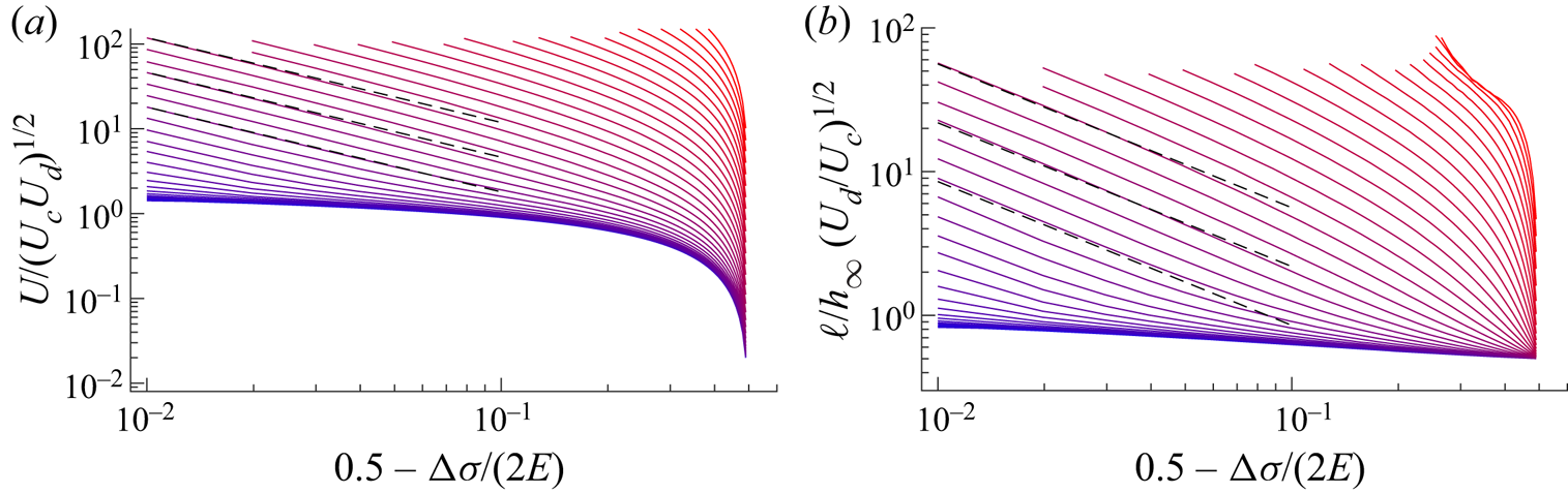
The main results of this paper are the following: (i) the films are shown to be governed by a perfectly reversible elastic law, with no influence of the shear or extensional interface viscosities. This proves that the viscoelastic response of the interface is not, as often assumed, the origin of the foam dissipation; (ii) we measure the relationship between the interface transfer velocity, from one film to its neighbour, and the tension difference between these films. We evidence a generic geometrical frustration at the meniscus: as it prevents the free transfer of the interface, this frustration is the origin of the largest part of the dissipation; (iii) we predict that this dominant dissipation is localized in a small part of the films that is close to the meniscus and that is sheared. In this domain, a well-controlled scale separation is used to simplify the hydrodynamics and transport equations, which become easily numerically solvable. One important prediction of our model is the scaling law for the length  $\ell$ of this sheared part of the film, as a function of the physico-chemical properties of the foaming solution. This length increases when the surfactant solubility decreases and is typically of the order of 100
 $\mathrm {\mu }$m. Importantly, it defines a boundary between the foams having bubbles smaller than
 $\ell$, in which the whole film should be sheared, and the foams having bubbles larger than
 $\ell$, in which the main film deformation should be an extension/compression. This reconciles the various classes of model, based either on extension or on shear, found in the literature.
On these bases, we built a model of foam viscosity for the large bubble regime and/or high surfactant solubility, e.g. for a bubble radius larger than  $\ell$. It reproduces the variations of the foam loss modulus as the square root of the frequency, and as the inverse of the bubble size, which are observed for a large class of foams (Krishan et al. Reference Krishan, Helal, Höhler and Cohen-Addad2010; Costa et al. Reference Costa, Höhler and Cohen-Addad2013b), and predicts the prefactor as a function of well-defined measurable, physico-chemical properties.
The paper is organized as follows. We first introduce the dedicated experimental set-up in § 2 and then describe the measurement of the relevant kinematic quantities in § 3. In § 4, we describe the technique used to measure the evolution of the tension of the five different films. In §§ 5 and 6 we build the constitutive relationships of the thin film and of the meniscus, respectively. In § 7, we unravel and model the dominant dissipation mechanism associated with the film/meniscus exchange and compare our model to the experiments in § 8. Finally in § 9 we discuss the relevance of our findings in a foam context and in § 10 we offer conclusions.
2. Experimental set-up and foaming solution
The same experimental set-up has been used previously in Bussonnière et al. (Reference Bussonnière, Shabalina, Ah-Thon, Le Fur and Cantat2020), and the measure of the kinematic properties of the film (velocity, extension) has already been presented in this former article for a restricted range of the control parameters. We recall here the main features and describe the physico-chemical properties of the solution.
2.1. Mechanical device
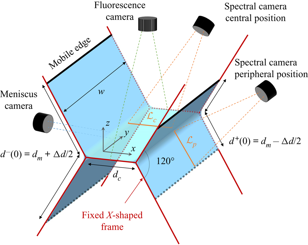
The film assembly is made of five foam films held by two metallic X-shaped pieces, as shown in figure 1. The central horizontal film has a width  $d_c=6$ mm and a length
 $W=41.5$ mm. The length has been chosen such that
 $W\gg d_c$, so the middle part of the central film is not influenced by the boundary effects on the solid frame. The short edges of the central film form menisci with the metallic frames (the supported menisci) while its long edges are menisci connected to the four peripheral films at an angle of 120
 $^{\circ }$ (the free menisci). The external edges of the peripheral films are connected to metallic pieces of length
 $W$ (black pieces in figure 1) which can translate along the lateral arms of the X-shape pieces. The mobile edge positions are controlled by four linear piezo motors (PI U-521.23). This geometry ensures that each film remains flat and stays in the same plane whatever the position of the motor, if the films are at mechanical equilibrium. Unless otherwise specified, an invariance in the
 $y$ direction will be assumed for all quantities. They are expressed as a function of the curvilinear abscissa
 $s$, defined for each film as the position along a line in the
 $(x,z)$ plane.
Schematic of the experimental set-up showing the mechanical device controlling film deformation and the different optical devices used to monitor the film motion.

As in Bussonnière et al. (Reference Bussonnière, Shabalina, Ah-Thon, Le Fur and Cantat2020), the deformation studied consists of a compression of the left peripheral films from an initial length  $d^{-}(0)=d_m+{\rm \Delta} d/2$ to
 $d^{-}=d_m-{\rm \Delta} d/2$ and a simultaneous symmetric extension of the right films from
 $d^{+}(0)=d_m-{\rm \Delta} d/2$ to
 $d^{+}=d_m+{\rm \Delta} d/2$ at a constant velocity
 $V$. In this study, we explore the influence of the motor velocity
 $V$, of the deformation amplitude
 ${\rm \Delta} d$ and of the mean position
 $d_m$.
2.2. Optical device
Three cameras are used to monitor the dynamics induced by the film deformations, as shown in figure 1. The meniscus camera records the size and vertical position of one free meniscus. It is magnified with a telecentric lens (Edmund Optics SilverTL × 4) and illuminated with a collimated white LED. The free menisci position in the  $(x,y)$ plane and the gross thickness variations of the central film are recorded with the fluorescence camera located on the top of the set-up. The fluorescein added in the foaming solution is excited with a 488 nm laser (Oxxius LBX 200 mW) and its emission is filtered using a band-pass filter. Finally, more precise thickness profiles
 $h$ are monitored along the line
 ${\mathcal {L}}_c$ in the central film or
 ${\mathcal {L}}_p$ in a peripheral film with a hyperspectral camera (Resonon Pika L). This camera, described in Bussonnière et al. (Reference Bussonnière, Shabalina, Ah-Thon, Le Fur and Cantat2020), measures the interfered spectrum intensity
 $I(\lambda )$ of the light emitted by a halogen lamp and reflected by the thin film. The thickness is extracted using the relation (Born & Wolf Reference Born and Wolf1999)
 \begin{equation} I(\lambda) \propto 1 - \cos\left(\frac{4{\rm \pi} h n}{\lambda} \left(1-\frac{\sin^{2}{\theta}}{n^{2}}\right)^{1/2}\right), \end{equation}
where  $n=1.33$ is the film refractive index,
 $\lambda$ the wavelength and
 $\theta$ the light incident angle. In our set-up,
 $\theta$ is
 $45^{\circ }$ for the central camera position and
 $58.5^{\circ }$ for the peripheral one.
2.3. Physico-chemical properties of the foaming solution
The foaming solution is a mixture of sodium dodecyl sulphate and dodecanol, that we chose to optimize the film rheological response. Some glycerol is added to improve the film stability and fluorescein is used to visualize the thickness patterns. To prepare the solution, the sodium dodecyl sulphate (SDS) ( $c_{{{SDS}}} =5.6$ g l
 $^{-1}$), the dodecanol (DOH) (
 $c_{{{DOH}}} =0.05$ g l
 $^{-1}$) and the fluorescein (
 $c_{{fluo}}=0.8$ g l
 $^{-1}$) are dissolved in a solution of distilled water–glycerol (15 % by volume). The equilibrium surface tension was measured at
 $\gamma _{0}= 33\pm 1$ mN m
 $^{-1}$ using the pendant drop method and the viscosity is
 $\eta = 1.5$ mPa s. Four needles located on the top mobile edges of the peripheral films can be used to supply solution to the film assembly during the entire experiment. Two sets of experiments have been performed, one where the foaming solution is injected at a rate of 0.2 ml min
 $^{-1}$ (0.05 ml min
 $^{-1}$ per needle) and one without injection.
Such a mixture has been extensively studied for its relevance in foam science and is thus well documented (see the review by Lu, Thomas & Penfold Reference Lu, Thomas and Penfold2000). However, its physico-chemical properties remain difficult to model due to the strong interactions between the anionic surfactant and the non-ionic alcohol, which can lead to the formation of a complex (Lu et al. Reference Lu, Purcell, Lee, Simister, Thomas, Rennie and Penfold1995; Nguyen & Nguyen Reference Nguyen and Nguyen2019; Vollhardt & Emrich Reference Vollhardt and Emrich2000; Kralchevsky et al. Reference Kralchevsky, Danov, Kolev, Broze and Mehreteab2003). Moreover, above the critical micelle concentration ( $\hbox{CMC}=2.33$ g l
 $^{-1}$ for pure SDS), DOH molecules can be solubilized in SDS micelles. These interactions lead to co-adsorption processes and mixed diffusion (Fang & Joos Reference Fang and Joos1992). As the chemistry has not been varied in this study, the potentially complex equation of state of the interface, adsorption and transport laws, taking into account the different species, cannot be addressed by our experimental results. We thus choose to keep our thermodynamic model of interface as simple as possible by linearizing the different laws.
Surface tension of pure SDS remains almost constant above the critical micelle concentration (Elworthy & Mysels Reference Elworthy and Mysels1966). The significant variations observed in our experiments are therefore assumed to be associated with the DOH only. At thermodynamic equilibrium, the surface tension  $\gamma _{th}$ is related to the DOH surface excess
 $\varGamma$ by
 \begin{equation} \gamma_{th}=\gamma_0+\left. \frac{\partial \gamma_{th}}{\partial \varGamma}\right|_{\varGamma_0}(\varGamma-\varGamma_0)=\gamma_0-E \frac{\varGamma-\varGamma_0}{\varGamma_0}, \end{equation}
with  $\gamma _0$ the surface tension of the foaming solution,
 $\varGamma _0$ the corresponding surface excess and
 $E=-({\partial \gamma _{th}}/{\partial \varGamma })|_{\varGamma _0}\varGamma _0$ the so called Gibbs–Marangoni elasticity. This elasticity can be estimated using the Langmuir model of DOH/micellar SDS solution proposed in Fang & Joos (Reference Fang and Joos1992) which leads to
 $E\approx 10$ mN m
 $^{-1}$ (see Appendix A).
The adsorption of DOH at the interface is characterized by
 \begin{equation} \varGamma=\varGamma_0+\left.\frac{\partial \varGamma}{\partial c}\right|_{c_0}(c-c_0)=\varGamma_0+h_{\varGamma}(c-c_0), \end{equation}
where  $c$ is the local dodecanol bulk concentration,
 $c_0$ the initial concentration and
 $h_{\varGamma }=({\partial \varGamma }/{\partial c})|_{c_0}$, hereafter called the reservoir length. Based on Fang & Joos (Reference Fang and Joos1992), we estimated
 $h_\varGamma \approx 5.4\ \mathrm {\mu }$m (see Appendix A). For processes faster than the micellization (Patist, Axelberd & Shah Reference Patist, Axelberd and Shah1998), we need to consider instead the equilibrium between the surface excess and the concentration
 $c^{m}$ of DOH in its monomer form, involving the parameter
 $h^{m}_\varGamma =({\partial \varGamma }/{\partial c^{m}})|_{c^{m}_0}\approx 370\ \mathrm {\mu }$m (see Appendix A).
The disjoining pressure as a function of the film thickness is also an important physico-chemical property of the system. However, it is negligible in our study as the films are always larger than 100 nm.
Finally, on each interface, we define  $\gamma (s)$ as the full interfacial stress which includes the surface tension
 $\gamma _{th}(\varGamma )$ as well as the potential contributions associated with the surface extensional and shear interfacial viscosities, respectively
 $\eta _s$ and
 $\kappa _s$. Note that the interfacial stress is thus a priori of tensorial nature, and
 $\gamma (s)$ represents its projection in the direction orthogonal to the direction of invariance
 $y$. For the thin films, we also define the film tension
 $\sigma$ that takes into account the contribution of both interfaces and of the film bulk (see § 4.2).
2.4. Control parameters and experimental protocol
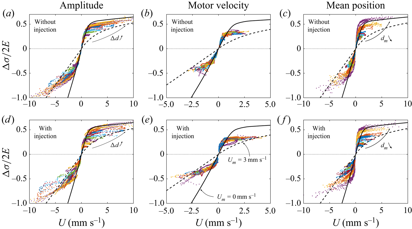
In this study we explored the influence of the deformation parameters on the film assembly dynamic by performing around 480 experiments.
A first experimental campaign was performed with the fluorescence camera used at a frame rate of 130 f.p.s., for  ${\rm \Delta} d$ varying between 2 and 12 mm,
 $V$ between 1 and 100 mm s
 $^{-1}$ and
 $d_m$ between 7 and 17 mm. Each set of parameters has been repeated at least 3 times with and without solution injection representing a total of 186 experiments. For some parameter values, the measurements have been refined in a second campaign, by increasing the frame rate to 300 f.p.s., increasing the number of experiments and/or using the spectral camera in the peripheral position, instead of the central position only.
The experimental protocol is as follows: a bucket full of foaming solution is placed on a motorized translation stage below the set-up. We first move the bucket up until the deformable frame is entirely immersed, then we move it down to produce the five films. This process leads to reproducible out of equilibrium films, rapidly draining under gravity. We let them evolve during 15 s before deforming the frame. The frame deformation is synchronized with the different cameras which record the film assembly dynamics during 30 s for the first campaign and 10 s for the second. Note that after the initial 15 s delay, the films are still out of equilibrium, but evolve on a time scale larger than the duration of the investigated deformation and relaxation. Moreover central (respectively peripheral) film remains thicker than 400 nm (respectively 1.5  $\mathrm {\mu }$m) during the entire experiment so the disjoining pressure is negligible in this study.
3. Determination of the kinematic quantities
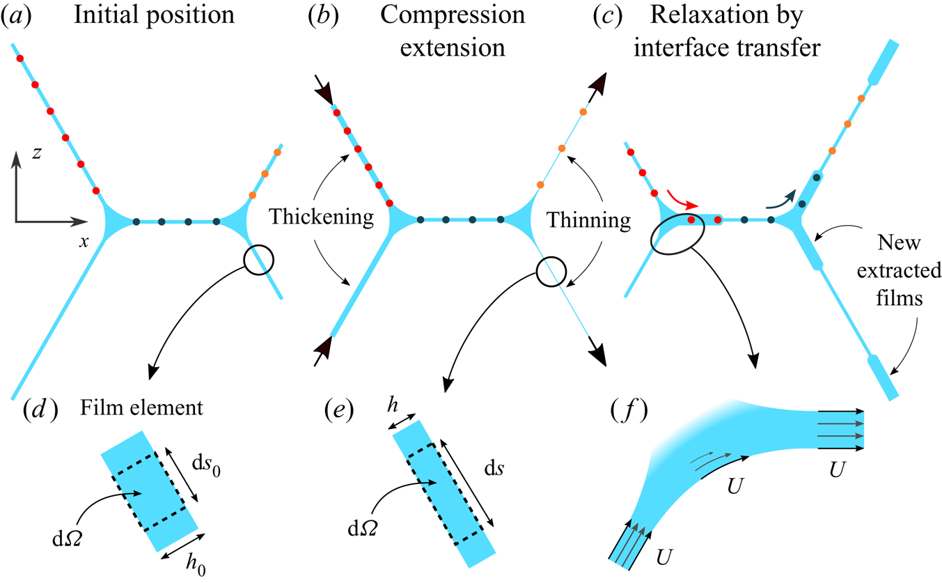
As shown in our previous study (Bussonnière et al. Reference Bussonnière, Shabalina, Ah-Thon, Le Fur and Cantat2020) and summarized in figure 2, the typical dynamics is composed of an extension of the peripheral films on the stretched side, and a compression of the peripheral films on the pushed side, at the first instants (figure 2b). The imposed deformation then relaxes through interface transfers between adjacent films (figure 2c). A visible signature of this transfer is the appearance of thick films, extracted from the menisci, in the central and stretched films.
(a–c) Schematic of the typical dynamics of the foam assembly. The coloured dots represent elementary material systems at the interface which are followed along their trajectories, thus illustrating film compression/extension as well as interface transfers from one film to the other. Films thicknesses evolve because of the compression/extension and because of the extraction of thick film from the menisci, associated with the interface transfers. (d,e) Zoom on a film element of volume  ${\rm d} \varOmega$ before and during the deformation. (f) Zoom on a meniscus showing the interface transfer dynamics, at velocity
 $U$.

3.1. Definition of the kinematic quantities
The extension of the films and the transfer velocity at the menisci are the two relevant kinematic quantities of the problem and they will be related to the film tensions through constitutive relationships in §§ 5 and 6. To properly define and measure the extensions and the transfer velocities we first clarify here different assumptions.
In the films, the relative velocity of the bulk phase with respect to the interfaces is a Poiseuille flow governed by the gravity forces and by the Laplace pressure gradients. As quantitatively discussed in § 6.2, these relative velocities are negligible far enough from the menisci, and the velocity can be assumed to be constant across the film (figure 2f). In the central part of each film, we can therefore define a film element  ${\mathcal {S}}$ as an elementary material system of volume
 $\textrm {d}\varOmega = h \, {\textrm {d}}S = h \,{\textrm {d} y} \, {\textrm {d}}s$ (see figure 2d,e) spanning the film from one interface to the other. It is a closed system which can be followed along its trajectory and which is entirely determined by the shape and position of its interface. The invariance in the
 $y$ direction imposes that
 ${\textrm {d} y}$ is constant. However, stretching or compression modifies
 ${\textrm {d}}s$. In such a film element, the film extension, or equivalently the interface extension, can be defined as
 \begin{equation} \varepsilon(t)=\frac{{\textrm{d}}s(t)}{{\textrm{d}}s_0} -1 = \frac{h_0}{h(t)}-1,\end{equation}
with  $h_0$ and
 $ds_0$ the initial characteristic of the film element, before deformation. The second equality is deduced from the volume conservation of the system, which imposes
 $h(t) \, {\textrm {d}}s(t)\, \textrm {d} y = h_0 \, {\textrm {d}}s_0 \,\textrm {d} y$. With this definition
 $\varepsilon > 0$ for an extension and
 $\varepsilon < 0$ for a compression.
The transfer velocity is a dynamical property associated with each free meniscus. In Bussonnière et al. (Reference Bussonnière, Shabalina, Ah-Thon, Le Fur and Cantat2020) we experimentally checked that, for the imposed deformation, when some film is extracted from one side of a free meniscus, a similar amount of film is absorbed on the other side, at the same rate, as schematized in figure 2(f). The surfactant monolayer slides on the meniscus interface, from one film to its neighbour, with negligible deformation. This allows us to define the transfer velocity  $U$ as, indifferently, the velocity of the film entering the meniscus at one side, the velocity of the film extracted on the other side or the velocity of the surfactant monolayer at the meniscus interface connecting both films. Experimentally,
 $U$ is measured in the central film. The model of § 7 goes beyond this first-order description and provides a prediction for the interface velocity difference between both sides of the free menisci, thus refining this first definition of the transfer velocity.
3.2. Measure of the transfer velocity
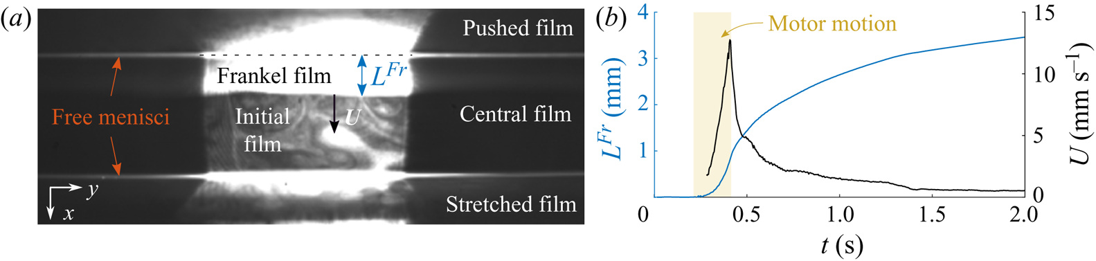
An image of the central film is shown in figure 3(a). In this film, the relaxation of the peripheral film deformation by interface transfer results in an extraction of a new film from the free meniscus on the compressed side (see figure 3a) and in a film entry in the free meniscus on the stretched side. The film extraction is governed by Frankel's theory (Mysels, Shinoda & Frankel Reference Mysels, Shinoda and Frankel1959; Bussonnière et al. Reference Bussonnière, Shabalina, Ah-Thon, Le Fur and Cantat2020) and the new film, called hereafter Frankel's film, is thicker than the remaining part of the film, which is the film initially present (denoted the initial film hereafter). Frankel's film therefore appears bright on the fluorescence camera, with a very well defined boundary at a distance  $L^{Fr}(t)$ from the pushed meniscus. The extraction begins as soon as the motors start and accelerates until the motors stop. The velocity is maximum at this time (figure 3b) and then the extraction slows down over a characteristic time scale of 1 s.
(a) Image of the fluorescence camera (top view) after the deformation showing the Frankel film extraction. This Frankel film is invariant in the  $y$ direction and the black parts on both sides are due to the fact that the illuminated domain size is smaller than
 $W$. (b) Typical Frankel film length
 $L^{Fr}$ (blue) and velocity
 $U= {\textrm {d}}L^{Fr}/ {\textrm {d}}t$ (black) evolution with time for
 ${\rm \Delta} d=10$ mm,
 $V=50$ mm s
 $^{-1}$ and
 $d_m=12$ mm. Yellow shaded area indicates when the motors move.

This motion occurs without compression or extension of the central film, which simply translates in the  $x$ direction (Bussonnière et al. Reference Bussonnière, Shabalina, Ah-Thon, Le Fur and Cantat2020). The central film dynamics is thus fully resolved by tracking the position
 $L^{Fr}(t)$ of Frankel's film boundary, with respect to the pushed meniscus position. For experiments recorded at a high frame rate (300 f.p.s.), the central film velocity is computed by smoothing the time derivative of
 $L^{Fr}$. For longer experiments with slower frame rate (130 f.p.s.), this velocity is extracted by first fitting the evolution of
 $L^{Fr}$ with a fourth-order polynomial during motor motion and a logarithm function after the motor stops. This uniform central film velocity is our experimental definition of the transfer velocity
 $U$, which happens to be identical at both free menisci, for the deformation we impose.
3.3. Measure of the film extension
The fact that the films may be absorbed by or extracted from the menisci implies that each individual film cannot be considered as a closed material system. Consequently, the distance  $d$ between the menisci on both sides of a film does not provide a measure of its extension
 $\varepsilon$.
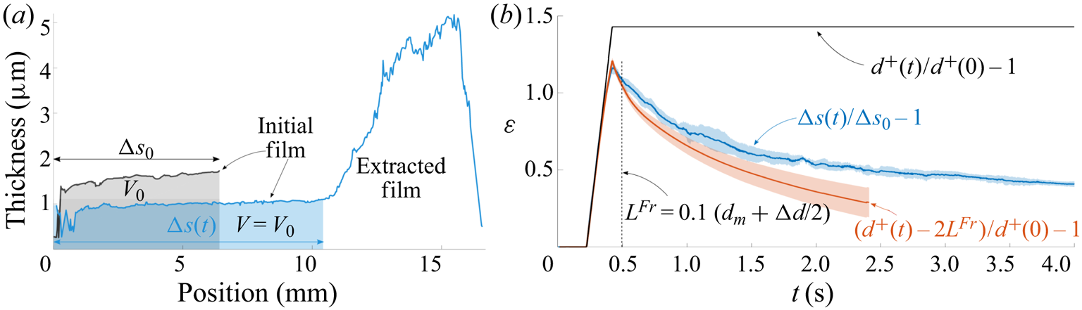
A first method to determine  $\varepsilon$ is based on thickness measurements. A film thickness profile in the stretched film, measured with the spectral camera, is shown in figure 4(a). After deformation we can see a thin part, corresponding to the initial film, in contact with a thicker part, corresponding to a newly extracted Frankel film, with a sharp transition between both. As shown in Bussonnière et al. (Reference Bussonnière, Shabalina, Ah-Thon, Le Fur and Cantat2020), a Frankel film is extracted both at the free meniscus (at the origin position in figure 4a) and at the supported meniscus, on the bottom right moving edge. However, gravity imposes a stratification of the non-horizontal films, and both Frankel films merge at the film bottom (Shabalina et al. Reference Shabalina, Bérut, Cavelier, Saint-Jalmes and Cantat2019), thus explaining the film profile. The key point here is that the initial film is a well-identified material system, which does not leave or enter the film during the experiment, and which is well separated from the Frankel film by a measurable boundary.
(a) Thickness profiles of the stretched bottom film at the initial time (black) and after the deformation (blue), as measured with the spectral camera between the right free meniscus (at the origin position) and the meniscus on the bottom right moving edge. The shaded areas correspond to the initial volume of the film (per unit length). (b) Extension as a function of time. Blue: film extension based on the thickness (see (3.2)); red: approximated film extension obtained from the transfer length  $L^{Fr}$ (see (3.3)); black: geometrical extension imposed by the motor positions. Averages (solid line) and standard deviations (shaded area) are calculated over 5 experiments for the thickness definition and 50 for the transfer length definition. The control parameters are
 ${\rm \Delta} d=10$ mm,
 $V=50$ mm s
 $^{-1}$ and
 $d_m=12$ mm. The dashed line delimits the validity range of the extension based on the transfer length.

To follow this material system, we proceed as follows: the volume  $V_0$ (per unit length in the
 $y$ direction) of the initial film is calculated by integrating the thickness profile at
 $t=0$ over the total length
 $d^{+}(0)={\rm \Delta} s_0$ of the film. During the dynamics, its length
 ${\rm \Delta} s(t)$ is deduced from the volume conservation: the thickness profile is integrated from the free meniscus at
 $s=0$ to the position
 ${\rm \Delta} s(t)$ at which the integral equals
 $V_0$. Note that, consistently,
 ${\rm \Delta} s(t)$ coincides with the position of the thickness transition, which is, however, known with a smaller precision.
As discussed in § 5.1, the extension is uniform in the film, thus allowing us to integrate (3.1) over the whole initial film to obtain
 \begin{equation} \varepsilon(t)=\frac{{\rm \Delta} s(t)}{{\rm \Delta} s_0} -1,\end{equation}
which is plotted in figure 4(b) as a function of time.
On the compressed side, the initial film is absorbed by the meniscus and the previous method unfortunately fails. Moreover, marginal regeneration plumes form at the bottom meniscus, move upward and merge with the film, draining the compressed film much faster than the other ones and making the extension measure based on (3.1) impossible. In that case, the actual size of the monolayer initially covering the film is estimated as  $d^{-}(t) + L^{Fr}_1(t) + L^{Fr}_2(t)$, with
 $d^{-}(t)$ the imposed film length at time
 $t$ and
 $L^{Fr}_1$ and
 $L^{Fr}_2$ the monolayer areas (per unit length in the
 $y$ direction) that have been lost by the compressed film respectively at the free meniscus and at the supported meniscus. As previously discussed, it is shown in Bussonnière et al. (Reference Bussonnière, Shabalina, Ah-Thon, Le Fur and Cantat2020) that
 $L^{Fr}_1 \sim L^{Fr}(t)$; at short times, we also observed that
 $L^{Fr}_2 \sim L^{Fr}(t)$. The same assumptions can be made for the stretched film to take into account the gain of area on both film sides. The extension can finally be estimated by, using the appropriate sign for each case,
 \begin{equation} \varepsilon(t)=\frac{d^{{\pm}}(t) \mp 2 L^{Fr}(t)}{d^{{\pm}}(0)} -1.\end{equation}
The values of  $\varepsilon$ in the stretched films, obtained using both definitions ((3.2) and (3.3)), are plotted in figure 4(b) for one series. As expected an excellent agreement is obtained at short times, but the two curves become different at longer times. Based on this comparison, we define a cutoff length
 $L_c= 0.1 (d_m+{\rm \Delta} d/2)$, represented by the dashed line in figure 4(b): for
 $L^{Fr}(t) < L_c$, the extension can be calculated using (3.3). Then
 $L^{Fr}_1$ and
 $L^{Fr}_2$ begin to significantly differ from
 $L^{Fr}$ and (3.3) becomes invalid.
In the following, the extension is computed for one parameter set using (3.2), in the stretched film and for the whole time range. For the other cases, extension and compression are computed with (3.3), at short times only, for  $L^{Fr}(t) < 0.1(d_m+{\rm \Delta} d/2)$. As this measure is much faster, it allows us to scan a large set of deformation parameters.
4. Determination of the film tensions
The set-up is designed so that, as long as the film structure is at equilibrium, the two free menisci stay at a constant position whatever the motor position. A meniscus motion is therefore the signature of some dynamical forces (Besson & Debrégeas Reference Besson and Debrégeas2007). We demonstrate in this section that the dominant forces are the tension differences between the films, which can therefore be modelled by a minimal surface of vanishing mean curvature during the dynamics. The position and shape of the free menisci, that we have extracted over time, can thus be used to measure the film tensions.
4.1. Meniscus motion
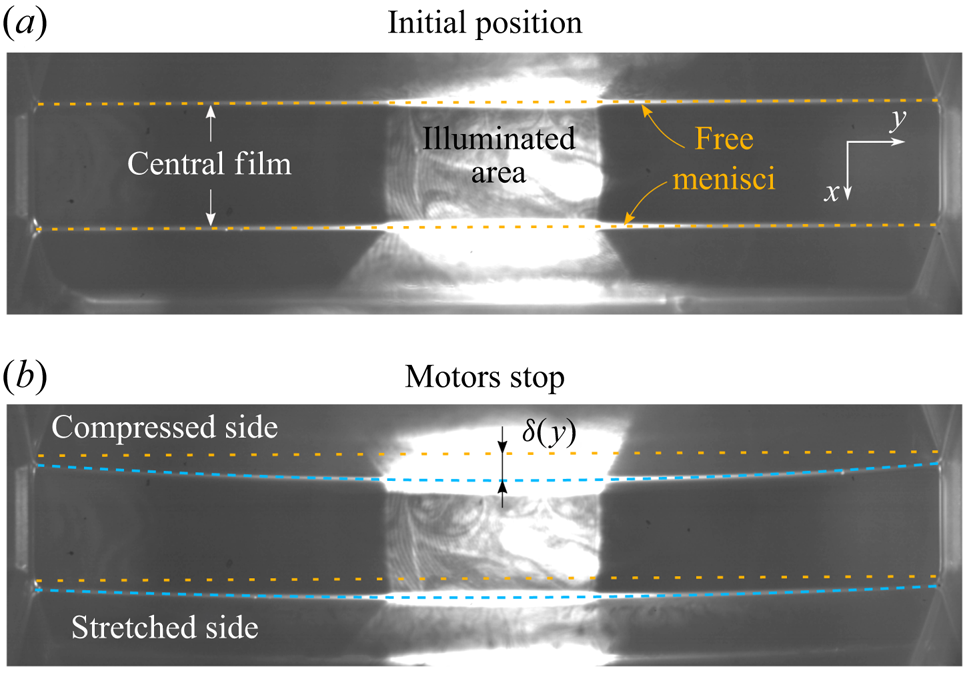
During the dynamics, both free menisci delimiting the central film move in the  $(x,y)$ plane toward the stretched side. As shown in figure 5, the meniscus ends slide on the solid frame and the whole meniscus curves in the direction of motion. The displacement
 $\delta ^{\pm }(y)$ of each free meniscus (the symbols
 $-$ and
 $+$ refer to the compressed and stretched sides, respectively) can be fitted at each time by a second-order polynomial, from which we deduce the sliding motion (the constant term
 $\delta _1^{\pm }$) and the meniscus curvature (from the quadratic term
 $\delta _2^{\pm }(y)$)
 \begin{equation} \delta^{{\pm}}(y)= \delta_1^{{\pm}} + \delta_2^{{\pm}}(y) = \delta_1^{{\pm}} + \delta_2^{{\pm}}(0) \left(1- \frac{2y}{W}\right)^{2} . \end{equation}
In this expression  $y=0$ is chosen in the middle of the film. The motion in the
 $z$ direction is measured with the meniscus camera (see figure 1) and is negligible.
(a) Fluorescence image of the central film at the initial state showing the position of the free menisci (yellow dashed line). (b) Fluorescence image at the end of the motor motion. New positions of the menisci are highlighted by dashed blue lines.

4.2. Estimation of the tangential forces and film tension definition
To estimate the value of the external forces acting on the films, we use the following orders of magnitude, corresponding to our observations: the film in-plane velocity scales as the transfer velocity  $U \sim 10^{-2}$ m s
 $^{-1}$, the film normal velocity scales as the meniscus velocity
 $U_m\sim 10^{-3}$ m s
 $^{-1}$, the film extension is up to
 $|\varepsilon | \sim 1$ and the fastest deformation time scale is
 $T \sim 10^{-1}$ s, corresponding to an extension rate
 $\dot {\varepsilon } \sim 10$ s
 $^{-1}$. Finally, we anticipate that the film tension differences between the different films
 ${\rm \Delta} \sigma$, that is deduced from the meniscus shape in § 4.5, are of the order of
 $10^{-3}$ N m
 $^{-1}$.
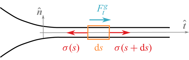
As shown in figure 6, we use on each thin film the normal and tangential unit vectors  ${\hat {\boldsymbol {n}}}$ and
 ${\hat {\boldsymbol {t}}}$, along the thin film profile (in the
 $(x,z)$ plane), associated with the spatial variables
 $\zeta$ and
 $s$, respectively. We define the film tension
 $\sigma (s) {\hat {\boldsymbol {t}}}$ as the force exerted by the film at an abscissa larger than
 $s$ on the film at an abscissa smaller than
 $s$. This quantity takes into account the interfacial stress
 $\gamma$ on both interfaces, and the contribution of the pressure in the liquid bulk, governed by the Laplace pressure (the latter term being negligible in the central part of each film). The tangential force balance on the piece of film located between
 $s$ and
 $s+ {\textrm {d}}s$ is
 \begin{equation} \rho \left( \frac{ \partial (h \langle u \rangle)}{\partial t} + \frac{\partial (h \langle u^{2} \rangle) }{\partial s} \right) = \frac{\partial \sigma}{\partial s} + \rho g_s h + F_t^{g} ,\end{equation}
with  $\rho$ the solution density,
 $g_s$ the gravity component along
 ${\hat {\boldsymbol {t}}}$,
 $\langle u \rangle$ the tangential velocity averaged in the normal direction, scaling as
 $U$, and
 $F_t^{g}$ the tangential stress due to the gas phase at both interfaces.
Schematic of a thin film with the tangential forces. The variable  $s$ in used along the direction
 $\hat {t}$ and the variable
 $\zeta$ along
 $\hat {n}$.

The first inertial term scales as  $\rho h U/T \sim 10^{-4}$ Pa, the weight as
 $\rho g_s h \sim 10^{-2}$ Pa (for the peripheral films) and the airborne stress as
 $F_t^{g} \sim \eta _g U/\delta _{bl}$, with
 $\delta _{bl}$ the thickness of the Blasius visco-inertial boundary layer,
 $\eta _g \sim 10^{-5}$ Pa s the gas shear viscosity and
 $\rho _g \sim 1$ kg m
 $^{-3}$ the gas density (Rutgers et al. Reference Rutgers, Wu, Bhagavatula, Petersen and Goldburg1996). The value of
 $\delta _{bl}$ is of the order of
 $\sqrt {\eta _g T/\rho _g} \sim 10^{-3}$ m (or
 $\sqrt {\eta _g d/(U \rho _g)}$ of similar order) and thus
 $F_t^{g} \sim 10^{-4}$ Pa. The convection term arises from the fact that we considered an open system and scales as
 $\rho h U^{2} /d \sim 10^{-5}$ Pa.
In the horizontal film, it results from these orders of magnitude that the Marangoni term  $\partial \sigma /\partial s$, also appearing in (4.2), cannot be larger than
 $10^{-4}$ Pa. Its variation between both ends of the film is thus below
 $10^{-6}$ N m
 $^{-1}$, which is much smaller than
 ${\rm \Delta} \sigma$. The surface tension variation induced by the gravity in each peripheral film simply balances its weight and is easily determined as
 ${\rm \Delta} \sigma ^{grav} \sim \rho g_s h d \sim 10^{-4}$ N m
 $^{-1}$, which is negligible too (and could be easily taken into account if needed).
One important consequence is that, in the parameter range we explored, the film tension is necessarily uniform on each thin film, whatever its physico-chemical properties (Durand & Stone Reference Durand and Stone2006). We thus define the film tension  $\sigma ^{-}$ in the two compressed peripheral films (top and bottom films are identical by symmetry, as gravity is negligible),
 $\sigma ^{+}$ in the two stretched peripheral films, and
 $\sigma ^{c}$ in the central film.
The contribution of both interfaces and of the film bulk to this film tension will be discussed in § 7. Note that, as tensions and extensions are related to each other, the tension uniformity validates the assumption of uniform extension in each given film made in § 3.3.
4.3. Estimation of the normal forces
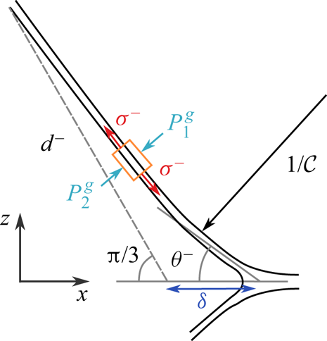
We now consider the normal motion of the peripheral films in order to show that they keep a negligible mean curvature during the deformation. Disregarding gravity effects (as discussed in § 4.2), the  $(x,y)$ plane is a symmetry plane, so the central film remains flat and stay in the
 $(x,y)$ plane. As shown in figure 7, the normal velocity of a piece of peripheral film is of the order of the meniscus velocity
 $U_m$. The Newton law in the normal direction applied to this system involves thus an inertial term (per unit film area) scaling as
 $I_f= h \rho U_m/T \sim 10^{-5}$ Pa. The normal forces are the gas pressures on both sides and the Laplace pressure, i.e. the normal component of the film tension contribution (Salkin et al. Reference Salkin, Schmit, Panizza and Courbin2016). The convection term is, as for the tangential projection, negligible.
Schematic of the pushed film with the normal forces applied.

In our set-up, the gas constitutes a continuous phase and the pressure variations are thus of dynamical origin only. The inertial gas pressure scales as  $P^{{g}}= \rho _g U_m^{2} \sim 10^{-6}\ \textrm {Pa} \ll I_f$. The gas phase can thus be assumed to be at rest. In the following, the atmospheric pressure is chosen as pressure reference and all the pressures defined in the liquid phase are the actual pressure minus this uniform atmospheric pressure.
The force balance thus only involves the film inertia  $I_f$ and the Laplace pressure
 $\sigma {\mathcal {C}}$. This provides a scaling law for the film mean curvature
 ${\mathcal {C}}$
 \begin{equation} {\mathcal{C}} \sim \frac{h \rho U_m}{\sigma T} \sim 10^{{-}3} \mbox{ m}^{{-}1}.\end{equation}
This mean curvature is much smaller than the observed curvature in the  $(x,y)$ plane, of the order of 20 m
 $^{-1}$ (see figure 5) and is therefore negligible. The peripheral films remain thus minimal surfaces of vanishing mean curvature, even during the motor motion, and their entire shape can be deduced from the position of their boundaries, i.e. from the position and shape of the free menisci.
4.4. Determination of the angles between the films
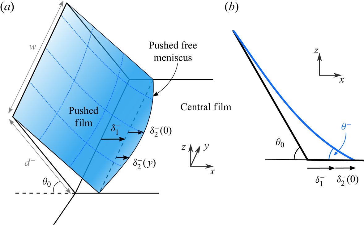
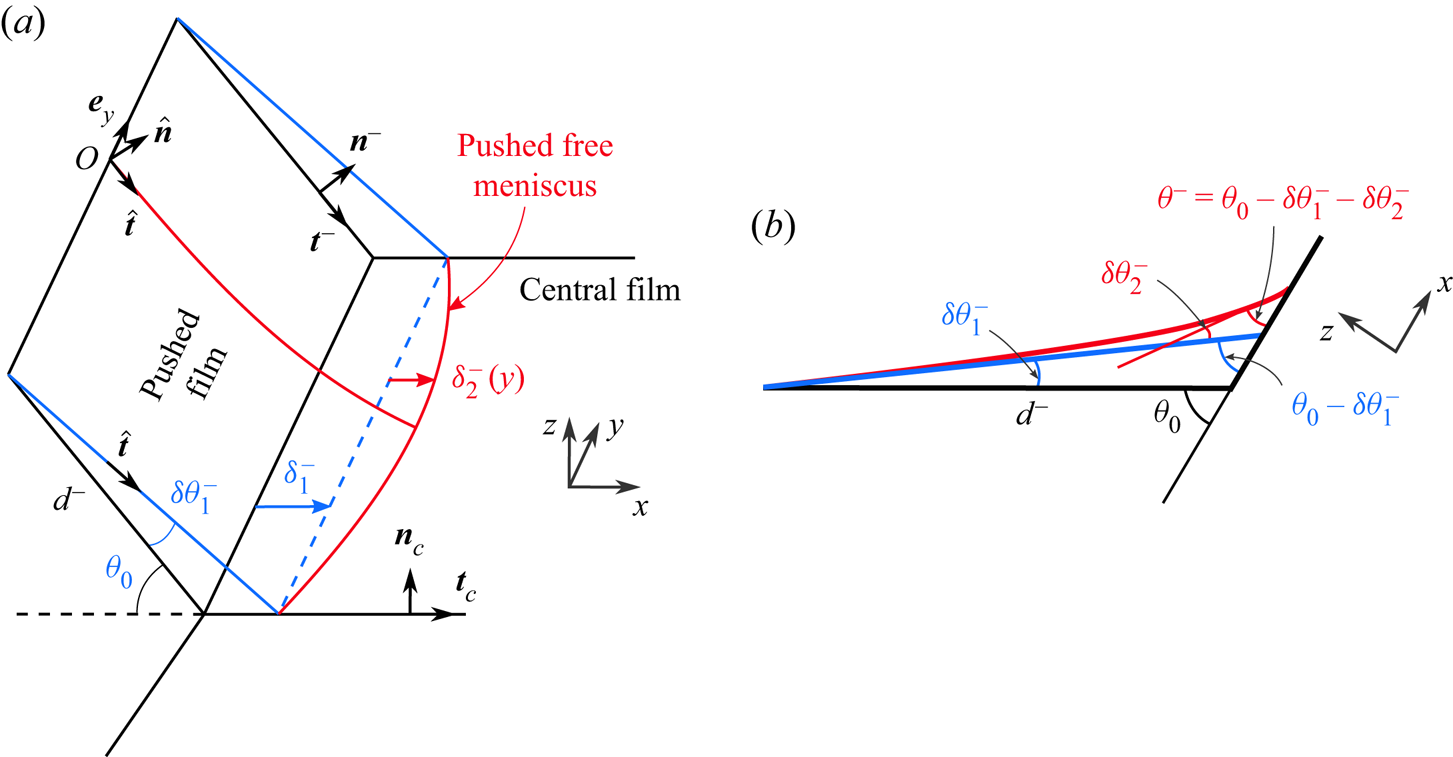
Figure 8 shows the scheme of the pushed film shape ensuring vanishing mean curvature and geometrical constrains (see also Embley & Grassia Reference Embley and Grassia2007). The relevant geometrical quantity is the angle  $2 \theta ^{-}$ (respectively
 $2 \theta ^{+}$) between the tangent vectors of the top and bottom pushed (respectively stretched) film, measured at the free meniscus position, in the
 $y=0$ plane (i.e. in the middle of the film). Its expression as a function of the free meniscus shape in the
 $(x,y)$ plane (figure 8) is derived in Appendix B and is given by
 \begin{equation} \theta^{{\pm}}=\tan^{{-}1}\left(\frac{d^{{\pm}}\sin\theta_0}{d^{{\pm}}\cos\theta_0+ \delta_1^{{\pm}}}\right)-\frac{\delta_2^{{\pm}}(0)}{w}\frac{{\rm \pi}\sin\theta_0}{\tanh \left(\dfrac{{\rm \pi} d^{{\pm}}}{w} \right)}. \end{equation}
The first term on the right-hand side is due to the meniscus sliding displacement ( $\delta _1$) and the second term is a correction induced by the meniscus curvature (
 $\delta _2$), as defined in (4.1). Note that, free menisci translate (displacement
 $\delta _1$) due to the finite frame thickness (1 mm) which allows peripheral films to accommodate such deformation. The initial equilibrium angle is
 $\theta _0={\rm \pi} /3$.
(a) Three-dimensional schematic of the pushed film shape ensuring zero mean curvature. (b) Cutting scheme of the pushed film at the middle of the film.

4.5. Determination of the film tensions
The film tensions  $\sigma ^{+}$,
 $\sigma ^{-}$ and
 $\sigma _c$ in the stretched, compressed and central films can now be obtained from the force balance on the meniscus. As the film tensions are uniform, they can be measured at any arbitrary point: we write the force balance on the elementary piece of free meniscus located around
 $y=0$ (middle of the film). Importantly, at this point, the plane
 $y=0$ is normal to the meniscus, so the tension forces acting on the system are in this plane. After a projection in the
 $x$ direction we get
 \begin{equation} \rho \alpha_{men} r_m^{2} \frac{{\textrm{d}}^{2} \delta^{{\pm}}(0,t)}{{\textrm{d}}t^{2}} ={\pm} ( 2 \sigma^{{\pm}} \cos \theta^{{\pm}} - \sigma_c ) , \end{equation}
with  $\alpha _{men} r_m^{2}$ the section area of the meniscus. The meniscus inertia scales as
 $\rho r_m^{2} U_m/T \sim 10^{-6}$ N m
 $^{-1}$ and is much smaller than
 ${\rm \Delta} \sigma$. We thus obtained the sought relationship
 \begin{equation} \sigma^{{\pm}} = \frac{\sigma_c}{2 \cos \theta^{{\pm}}},\end{equation}
with  $\theta ^{-}$ and
 $\theta ^{+}$ expressed as a function of the meniscus displacement in (4.4).
We show in the next section that any variation of film tension is associated with a film extension  $\varepsilon$. As the central film is never stretched or compressed, we can assume
 $\sigma _c = \sigma _0 = 2\gamma _0$. The film tension variations in the stretched and compressed peripheral films, with respect to their equilibrium values, are thus given by
 \begin{equation} \frac{{\rm \Delta} \sigma^{{\pm}}}{ \sigma_0} = \frac{1}{2 \cos \theta^{{\pm}}}-1. \end{equation}
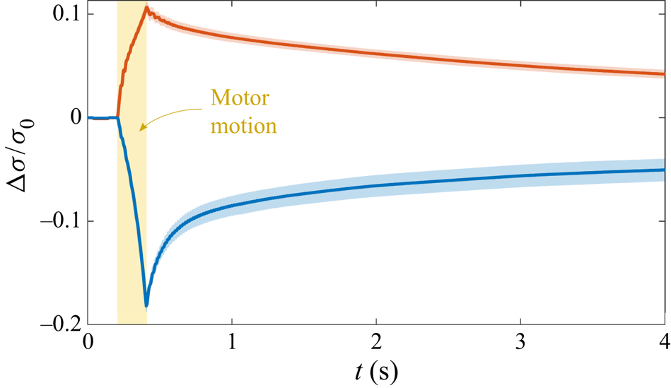
An example of film tension variation is shown in figure 9 as a function of time. We find, as anticipated, an order of magnitude of a few mN m $^{-1}$ for
 ${\rm \Delta} \sigma$. As soon as the motors start, the film tension begins to deviate from its equilibrium value. It reaches a maximum/minimum when the motors stop and then relaxes.
Typical time evolution of the film tension variation of the stretched (in red) and compressed (in blue) sides for  ${\rm \Delta} d=10$ mm,
 $V=50$ mm s
 $^{-1}$ and
 $d_m=12$ mm. Solid lines (respectively shaded areas) represents the average (respectively the standard deviation) over 50 experiments. These values are deduced from the meniscus displacement using (4.4) and (4.6).

Note that, by symmetry, the final state reached by the system is identical to its initial state. The total amount of dissipated energy  ${\mathcal {D}}$ (per unit length) is therefore the total work provided by the motor to the system
 \begin{equation} {\mathcal{D}} = V \int_0^{t_m} 2 (\sigma^{+} - \sigma^{-}) \, {\textrm{d}}t ,\end{equation}
with  $V$ the motor velocity and
 $[0-t_m]$ the duration of the motor motion. The tension difference between the stretched and compressed films is thus a direct signature of the system dissipation.
5. Constitutive relation for the film
In the previous sections we determined the tension and the extension of the different films, which now allows us to build the film experimental constitutive relation, i.e. the relationship between the two quantities.
5.1. Experimental results
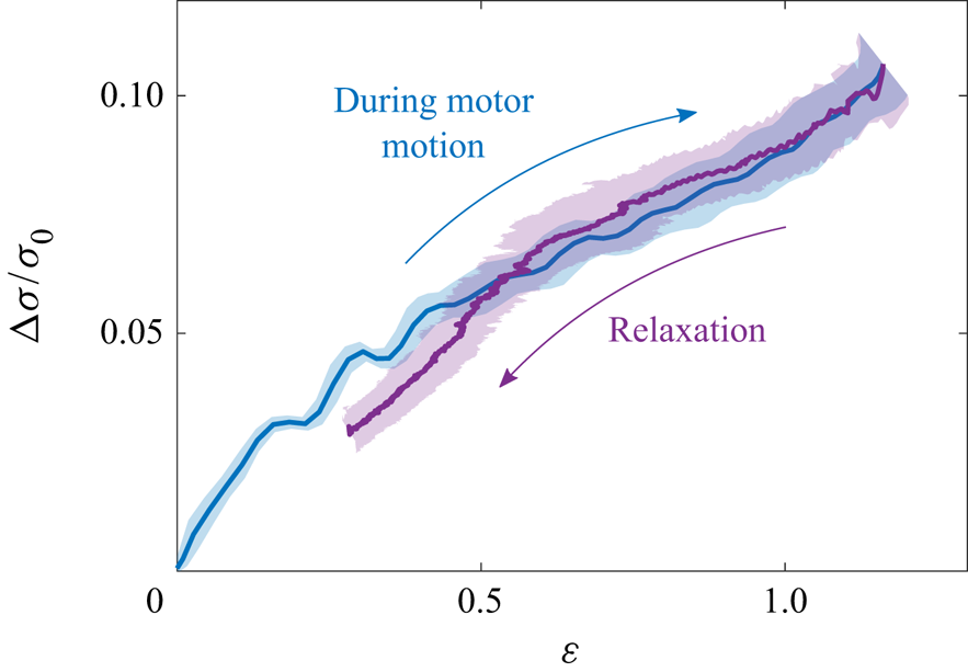
We first plot, in figure 10, the tension variation in term of the film extension for the experiments where the extension has been deduced from the thickness measurements in stretched films. This allows us to monitor the relationship over the entire experiment, during 10 s. The film is first stretched (blue data) and then relaxes toward its initial length (purple data). The most noticeable result of the paper is that the two parts of the curve are perfectly superimposed, thus proving unambiguously the purely elastic behaviour of the film.
Film tension relative variation as a function of  $\varepsilon$ deduced from the film thickness (using (3.2)) during the motor motion (blue) and after motor stops (purple) for
 ${\rm \Delta} d=10$ mm,
 $V=50$ mm s
 $^{-1}$ and
 $d_m=12$ mm. The solid lines (shaded areas) represent the averages (standard deviations).

To investigate further the role of the extension rate, we varied the motor motion parameters in a large range. The amount of data was too large to use the definition (3.2) of the extension (which requires manual check during the data processing) and we used the definition (3.3) instead, for the stretched and compressed films, at short times (i.e. during motor motion and just after).
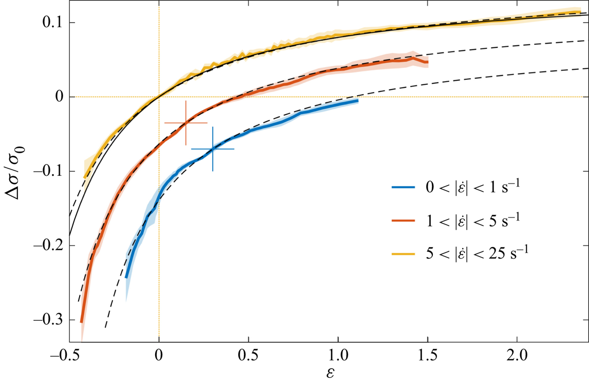
At each time, for each experiment and each film, we measure the data set ( $\varepsilon , \dot {\varepsilon }, \sigma$). All data points are then considered together, whatever the values of the control parameters. They are binned by extension rate
 $|\dot {\varepsilon }|$, and averaged. The bins have been chosen to show the whole range of extension rate while keeping a significant number of points in each bin. Most of the points are associated with a small
 $|\dot {\varepsilon }|$, but there are still 8500 data points for the
 $[5 ; 25]$ s
 $^{-1}$ bin.
The obtained results are shown in figure 11. Negative  $\varepsilon$ corresponds to a compression and positive
 $\varepsilon$ to an extension. Note that to provide a better readability of the data, we shifted the
 $x$ and
 $y$ axis of the two lowest extension rates. The three curves would otherwise be perfectly superimposed, as indicated by the theoretical law (dashed black lines) plotted on each graph, which is each time the same curve. For the investigated parameters, i.e.
 $|\dot {\varepsilon }|$ in the range
 $[0 ; 25]$ s
 $^{-1}$ and
 $\varepsilon$ in the range
 $[-0.5 ; 2]$, the film tension is thus a function of the extension only. The relationship between both quantities is discussed in the next section, on the basis of the classical models.
Film tension relative variation as a function of the local film extension  $\varepsilon$. Each colour corresponds to the average over all the data having an extension rate in a given range. The 3 curves are perfectly superimposed and the red and blue curves have been shifted for the sake of visibility: the corresponding axis origins are the cross of the same colour. The error bar (shaded area) is the standard deviation and is less than
 $10\,\%$ on average. The dashed lines are 3 copies of the same curve: the theoretical prediction of (5.5), with the relative elasticity
 $E/\gamma _0=0.16$. The solid line corresponds to the nonlinear model using Langmuir adsorption of reference (Fang & Joos Reference Fang and Joos1992), derived in Appendix C, with an initial DOH concentration of
 $0.6 c_0$.

5.2. Gibbs–Marangoni elasticity
The full interfacial stress  $\gamma$ of an interface involves the thermodynamic definition of the surface tension
 $\gamma _{th}$ which depends solely on the local surfactant interfacial excess (
 $\varGamma$) and the intrinsic surface extensional and shear viscosities, respectively
 $\kappa _s$ and
 $\eta _s$. In our
 $y$-invariant geometry, similar to a Langmuir trough geometry, this stress is (Edwards, Brenner & Wasan Reference Edwards, Brenner and Wasan1991; Stone Reference Stone2010)
 \begin{equation} \gamma = \gamma_{th}(\varGamma(s)) + (\eta_s + \kappa_s) \dot{\varepsilon} .\end{equation}
The local surface excess might deviate from its initial equilibrium value and depends on the surfactant transport processes. In the general case, the surfactant advection–diffusion and the exchanges between the bulk and the interface result in an elastic and an apparent viscous behaviour due to, respectively, the in-phase and out-of-phase (delayed) response of the surface excess with the deformation.
Here, the diffusion time scales of the surfactants in the directions parallel or transverse to a thin film scale as  $\tau ^{p} \sim d^{2}/D \sim 10^{6}$ s and
 $\tau ^{t} \sim h^{2}/D \sim 10^{-2}$ s, respectively, whereas the experimental time scale is of the order of 1 s. This scale separation allows us to assume that (i) there is no diffusive transport along the film; (ii) at a given location
 $s$ in the film, the equilibrium between the bulk concentration and the interface excess is immediately reached. From these assumptions, and following Prins, Arcuri & Van Den Tempel (Reference Prins, Arcuri and Van Den Tempel1967) and Couder, Chomaz & Rabaud (Reference Couder, Chomaz and Rabaud1989), we can deduce the relation between the surface excess and the film extension.
As established in § 4, the film tension  $\sigma$ is homogeneous in each film. However, some important dynamical processes, discussed in § 7, occur close to the meniscus and lead to variations of the interface tension
 $\gamma$ on both film interfaces, while keeping the resulting film tension constant. Here, we focus on the central part of the films, where the bulk pressure is the reference pressure, both interface tensions are identical and the velocity field across the film is homogeneous (see § 6.2 for more details). In this domain we thus simply have
 $\sigma = 2 \gamma$. Moreover, the interface
 ${\textrm {d}}S(t)$ of a film element
 $\mathcal{S}$ of volume
 $d\varOmega = h(t) \, {\textrm {d}}S(t)$ is always in contact with the same liquid bulk. At our experimental time scale
 $\tau ^{t} \ll T \ll \tau ^{p}$, we can thus assume that (i) the film element
 ${\mathcal {S}}$ is a closed system (both for the liquid phase and for the surfactants); (ii) the bulk concentration
 $c$ has a homogeneous value
 $c_0+ {\rm \Delta} c$ in
 $d\varOmega$ and is at equilibrium with the interface concentration, so that
 $\varGamma =\varGamma _0+h_\varGamma {\rm \Delta} c$ (see (2.3)). The surfactant mass conservation leads to (Prins et al. Reference Prins, Arcuri and Van Den Tempel1967; Couder et al. Reference Couder, Chomaz and Rabaud1989)
 \begin{equation} \varGamma= \varGamma_0 \frac{1 + h_0/(2 h_\varGamma)}{1+\varepsilon + h_0/(2 h_\varGamma)}. \end{equation}
The surface tension  $\gamma _{th}$ is related to the local surface concentration through (2.2) and, using (5.2), the interfacial stress in (5.1) becomes
 \begin{equation} \gamma = \gamma_0 + E \frac{\varepsilon}{1+\varepsilon + h_0/(2 h_\varGamma)}+(\eta_s + \kappa_s) \dot{\varepsilon}. \end{equation}
Finally, the relative film tension variation is predicted to be
 \begin{equation} \frac{{\rm \Delta}\sigma}{\sigma_0} =\frac{\sigma^{{\pm}}-\sigma_c}{\sigma_c} = \frac{E}{\gamma_0}\ \frac{\varepsilon}{1+\varepsilon + h_0/(2 h_\varGamma)}+\frac{(\eta_s + \kappa_s)}{\gamma_0}\ \dot{\varepsilon}.\end{equation}
This prediction is plotted in figure 11, using  $\kappa _s+\eta _s=0$,
 $h_0/h_\varGamma =0$ and
 $E/\gamma _0=0.16$ as fitting parameters. The agreement with experimental data is excellent for the whole range of deformation and deformation rate explored, and the constitutive relation for the films is thus
 \begin{equation} \sigma= \sigma_0 + 2 E \frac{\varepsilon}{1+\varepsilon}.\end{equation}
A first important consequence of this agreement with the experiments is that the films do not exhibit any measurable viscous behaviour, neither intrinsic nor effective. The potential viscous contribution is actually hidden by the experimental error estimated at approximately 0.5 mN m $^{-1}$. The viscous term is thus below 0.5 mN m
 $^{-1}$ for extension rates reaching
 $\dot {\varepsilon }\approx 10$ s
 $^{-1}$, which provides the upper limit for the surface viscosities
 $\kappa _s+\eta _s\le 5 \times 10^{-5}$ kg s
 $^{-1}$. This result is consistent with different measurements reported in the literature (Wantke, Fruhner & Örtegren Reference Wantke, Fruhner and Örtegren2003; Drenckhan et al. Reference Drenckhan, Ritacco, Saint-Jalmes, Saugey, McGuinness, Van der Net, Langevin and Weaire2007; Zell et al. Reference Zell, Nowbahar, Mansard, Leal, Deshmukh, Mecca, Tucker and Squires2014). Therefore, the dissipation observed in our experiments cannot be attributed to the viscosity of the interface.
A good fit of the experimental results by (5.4) is obtained for a large range of  $h_\varGamma$ (
 $5\ \mathrm {\mu }$m
 $< h_{\varGamma }<\infty$) while the relative elasticity remains in a narrow range
 $0.16< E/\gamma _0<0.18$ corresponding to an elasticity
 $E\approx 5\text {--}6$ mN m
 $^{-1}$. This indicates that the film tension variation arises from insoluble surfactants (significant
 $h_\varGamma$) and validates our assumption that the DOH is at the origin of the observed tension variations. SDS molecules are mainly passive to the deformation due to the high bulk concentration as well as the fast adsorption/desorption dynamic of the order of
 $1\ \textrm {ms} \ll T$ (Chang & Franses Reference Chang and Franses1992).
The elasticity  $E$ extracted from the experiments is close to the one estimated by using the physico-chemical model of Fang & Joos (Reference Fang and Joos1992) (
 $E^{th}= 10.6$ mN m
 $^{-1}$, see Appendix A). However,
 $E$ is slightly lower than this estimated value. This deviation may be due to the fact that the DOH is depleted during the film formation. Such a DOH depletion would indeed results in a decrease of the elasticity, in agreement with the experimental trend.
A refined model based on the nonlinear Langmuir adsorption (see Appendix C) gives also a good fit of the experiment, assuming depletion of DOH from  $c_0$ to
 $0.6 c_0$ during the initial film formation, as shown by the solid line in figure 11. At the present, it is not possible to discriminate between the different models of adsorption isotherms, nor to determine
 $h_\varGamma$. In the following, for the sake of simplicity, we choose the simplest linear model with
 $E/\gamma _0=0.16$ obtained in the limit
 $h_\varGamma \rightarrow \infty$. Note that this choice introduces only a small error on
 $E$, as
 $h_\varGamma$ is much larger than
 $h_0$ and thus has little influence on the fit.
6. Flow properties in the meniscus and around
As shown in the previous section, the thin films far from menisci confer a pure elastic behaviour to the foam assembly. In this section, we show that the viscous, dissipative, behaviour arises from a generic geometrical frustration at the meniscus.
6.1. Experimental relationship between the transfer velocity and the tensions
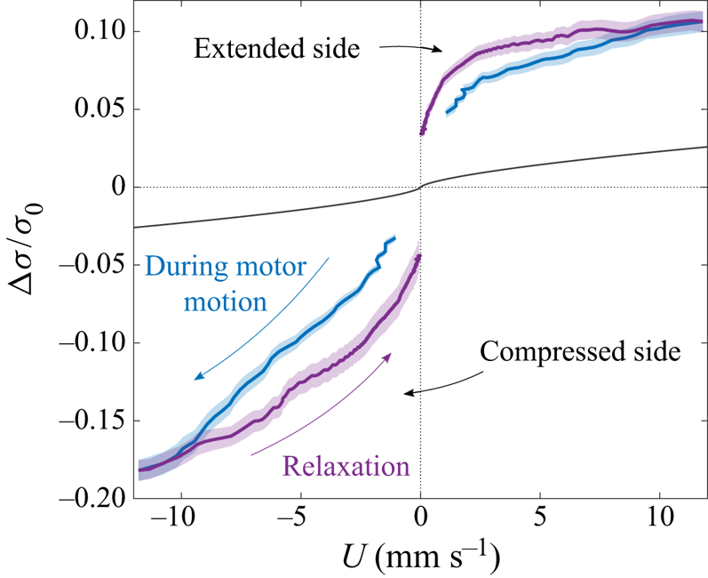
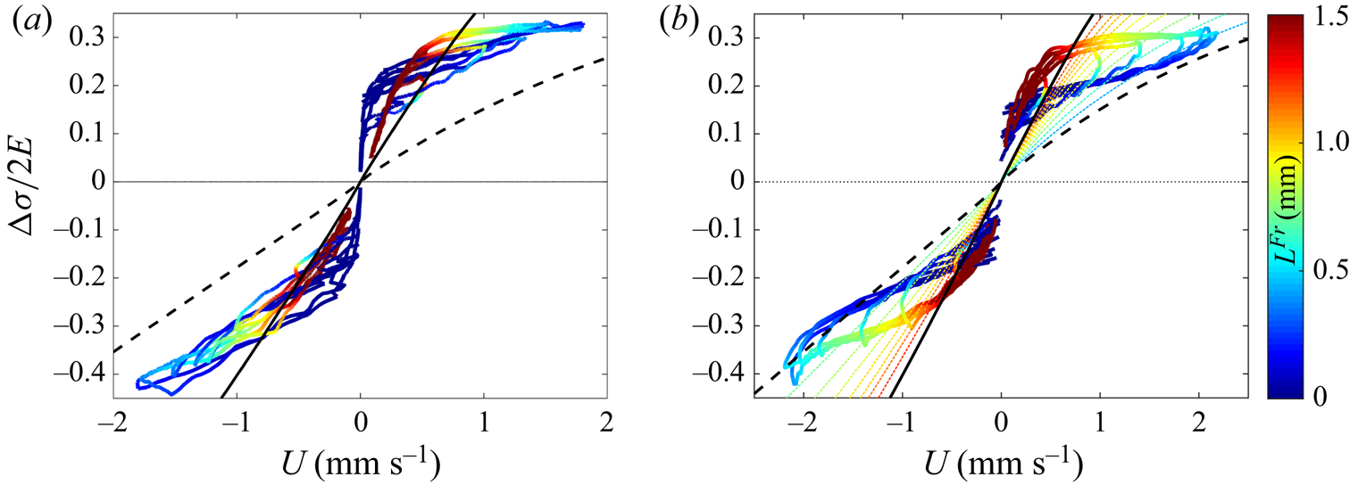
A surface tension difference between films arises from the extension/compression of the peripheral films at short times, and this tension difference tends to relax through interface transfer from one film to its neighbour at later times. Figure 12 shows the experimental relationship between the tension difference and the transfer velocity, i.e. the observed viscous response of the film assembly. By convention, the velocity  $U$ is positive on the stretched side, and negative on the compressed one.
Relative film tension variation in term of the transfer velocity  $U$ for
 ${\rm \Delta} d =10$ mm,
 $V=50$ mm s
 $^{-1}$ and
 $d_m=12$ mm. Solid lines (shaded areas) represent the averages (standard deviations) over 50 experiments, respectively in blue and purple for the short times (during the motor motion) and the long times (after the motors stop). The black line is the theoretical tension relative variation associated with a Frankel film extraction at velocity
 $U$, given by (6.6).

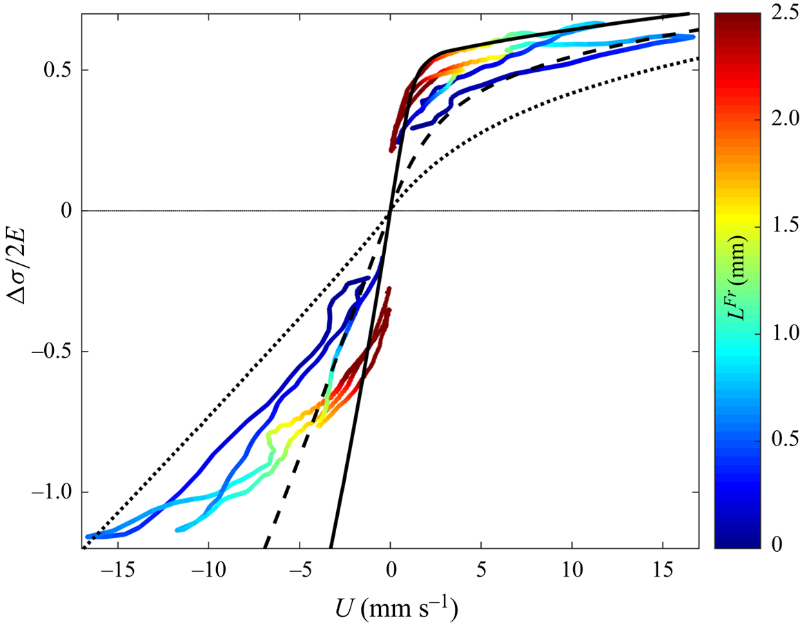
The surface tension evolution is asymmetric between the compressed and stretched sides: on the stretched side, surface tension rises rapidly with the transfer velocity and seems to reach a plateau at  ${\rm \Delta} \sigma /\sigma _0\approx 0.1$; on the compressed side, tension keeps decreasing at higher velocity. The curves obtained during the motor motion and afterwards, are qualitatively the same. Similar plots are obtained for our whole parameter set (see § 8). So, in a first approximation, there is a relationship between
 ${\rm \Delta} \sigma$ and
 $U$, which plays the role of a constitutive relation for the meniscus.
However, the tensions (in absolute value, and for a given velocity) are significantly smaller during the motor motion than during the relaxation, for both sides, and  $U$ does not depend uniquely on
 ${\rm \Delta} \sigma$. Anticipating the results of the model of § 7, this feature can be explained by a transition between two regimes: at short times the menisci are good surfactant reservoirs and limit the surfactant concentration variations at the interfaces; then the bulk concentration departs from its initial value in the meniscus subphase (meniscus saturation or depletion), allowing for larger concentration gradients at the interface and thus for larger tension differences. This is at the origin of the hysteresis observed in figure 12. The precise localization in the film/meniscus structure of these tension gradients is governed by the complex coupling between the hydrodynamics and transport processes described in § 7.
Note that, as the interface transfer is the process allowing the relaxation of the elastic energy stored in the peripheral films, it is a dissipative process. The only dissipative features in the system are the viscous and diffusive transports, the first contribution scaling as the square of the velocity gradients, and the second as the square of the concentration gradients. The dissipative processes in the central part of the peripheral films have been shown to be negligible in the § 5: the interface and bulk viscosities do not contribute to the dynamics, and the diffusion in the films is either to fast or to slow to induce a significant dissipation. The dissipation is thus localized in the menisci or in their vicinity, as shown below.
6.2. Meniscus frustration – domain definitions
The prediction of the relationship between the velocity transfer and the tension difference between adjacent films first requires us to analyse where the tension gradients are located. This is performed using specific approximations in the different domains defined in this section.
The surface tension variation along an interface is related to the bulk velocity  $v(s,\zeta )$ beneath it through the continuity of the tangential stress. We showed in § 4.2 that air drag is negligible and the stress continuity thus simplifies into the Marangoni relation
 \begin{equation} \frac{\partial \gamma}{\partial s}={\pm} \eta\frac{\partial v}{\partial \zeta}. \end{equation}
respectively for the interface at  $\zeta >0$ and for the one at
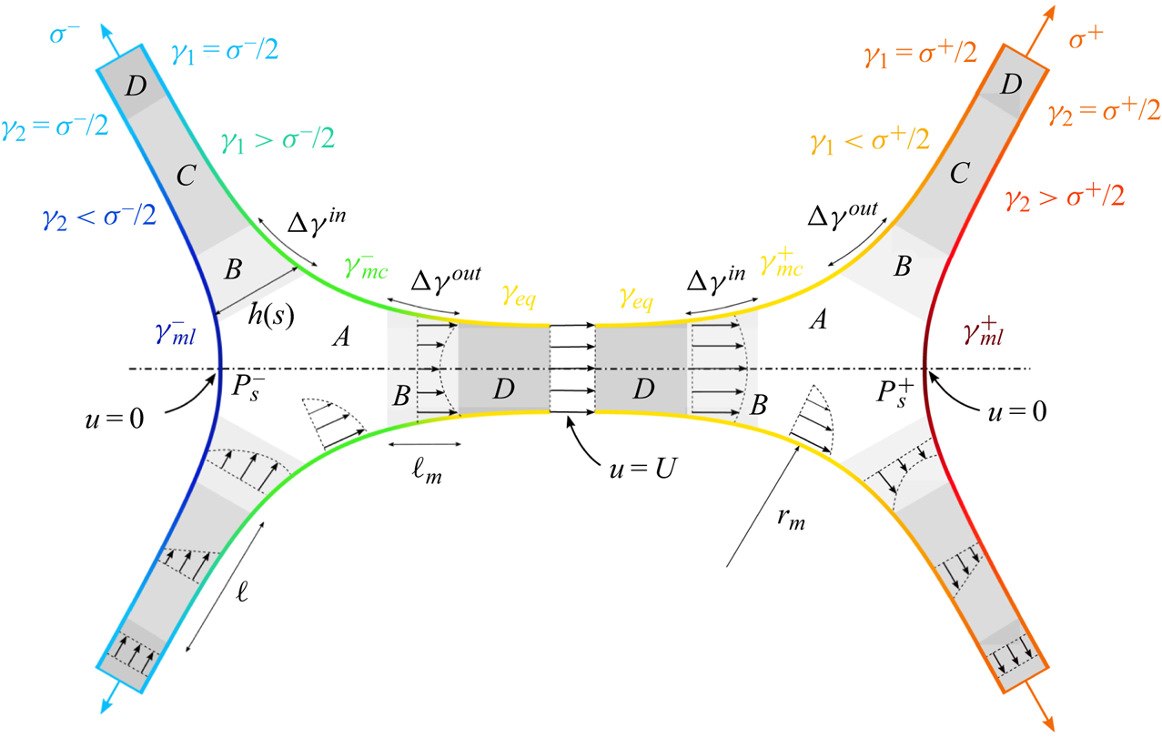
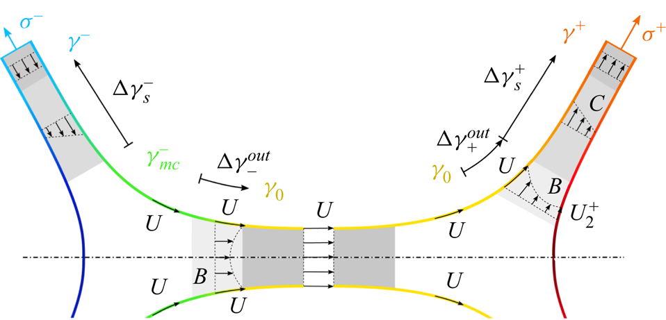
 $\zeta <0$ (see the notation convention in figure 6). The variation of the surface tension is thus coupled to the flow profile which depends on the liquid confinement. Figure 13 represents the different domains and their corresponding flow profiles. Note that the schematic is not to scale for clarity and that the central film size, the meniscus radius of curvature and the film thickness verify
 $d_c \gg r_m \gg h$.
Schematic of the velocity profiles and of the different domains. The interface colour codes for the surface tension: the lower value is  $\gamma _{ml}^{-}$ in dark blue and the higher value is
 $\gamma _{ml}^{+}$ in dark red.

The domain A is usually called the static meniscus, in which the curvature remains close to the equilibrium one. Elsewhere, the liquid is confined in thin films characterized by a thickness profile  $h(s)$, in which
 $\partial _s h \ll 1$ so that the classical lubrication approximations apply. One important consequence is that the pressure in the films does not depend on
 $\zeta$ and is only controlled by the Laplace pressure
 \begin{equation} P(s)={-} \frac{\gamma_0}{2} \partial_{ss}h,\end{equation}
with  $\partial _{ss}h/2$ the curvature of each interface. The reference surface tension
 $\gamma _0$ is used in this expression as tension variations would lead to higher-order corrections. The film tension
 $\sigma$, defined in figure 6, is the sum of both film interface tensions
 $\gamma _1(s)$ and
 $\gamma _2(s)$, and of the action of the pressure,
 $-P(s) = (\gamma_0/2) \partial_{ss} h$, integrated over the film thickness
 $h(s)$
 \begin{equation} \sigma(s) = \gamma_1(s) + \gamma_2(s) + \frac{\gamma_0}{2} h(s) \partial_{ss}h .\end{equation}
The domain B, usually called the dynamical meniscus, of extension  $\ell _m$, is defined as the part of the films in which the Laplace pressure is non-negligible. It connects the static meniscus at low pressure to the films at reference pressure. A Poiseuille flow results from the Laplace pressure gradient, which controls the volume exchanges between the films and the meniscus.
The domain D is the central part of the film, where the only degree of freedom is a stretching/compression deformation. The tensions satisfy  $\gamma _1=\gamma _2=\sigma /2$ and the velocity field is a plug flow. The film elements used in the previous section can only be defined in this domain.
The novelty of our approach is to define the domain C, of length  $\ell$, between the domains B and D, in which the Laplace pressure is negligible, but the tensions on both film sides are different. The tensions
 $\gamma _1(s)$ and
 $\gamma _2(s)$ are equal by symmetry in the central film but may indeed differ in the peripheral films.
These domains are called the sheared film in the following. They arise from a mismatch of surface velocity appearing on the peripheral films in the vicinity of the meniscus, due to a geometrical frustration. On the stretched side for example, the interface coming from the central film slips almost freely over the meniscus whereas, on the other interface, the velocity must vanish on the symmetry plane (at the point  $P_s^{+}$ in figure 13). This results in the shearing of the thin film close to the meniscus and in a tension difference between both interfaces. This domain C is far enough from the meniscus for the Laplace pressure to be negligible, but close enough from it so that the boundary condition difference on both interfaces is not screened. Such behaviour has already been observed and quantified for a meniscus in contact with a solid wall (Cantat Reference Cantat2011; Reichert, Cantat & Jullien Reference Reichert, Cantat and Jullien2019), and was conjectured in Petit (Reference Petit2014) for a free meniscus.
Note that this geometrical frustration is not specific to our deformation, and is a generic feature for any meniscus connected to three (or any odd number of) films: it is not possible to impose a uniform velocity on each of the three meniscus interfaces without getting a velocity difference between both interfaces in at least one film.
The sizes of each domain are solution of the hydrodynamical problem and a priori depend on the physico-chemical properties of the solution. However, from our experimental observations, we assume that the sheared film length is much larger than the dynamical meniscus length, and much smaller than the peripheral film size, thus leading to the condition  $d^{\pm } \gg \ell \gg \ell _m$, which allows us to separate the regions
 $B$,
 $C$ and
 $D$. These conditions will be discussed and verified in § 7. The approximations relevant for each domain are discussed below.
6.3. Tension in the static menisci – domain A
On each of the three interfaces of the static meniscus, the surface tension variation is given by the flow profile in the bulk through (6.1). The length over which the bulk velocity  $v$ varies in the normal direction is a priori unknown, and can be much smaller than the meniscus size
 $r_m$, thus potentially leading to high velocity gradients. In that case, this length should be the viscous boundary layer thickness
 $\ell _{vbl}$ given by
 \begin{equation} \ell_{vbl}^{st}=\sqrt{\frac{\eta r_m}{\rho U}} \ \mbox{or} \ \ell_{vbl}^{tr}=\sqrt{\eta T/\rho} , \end{equation}
respectively for the steady case and the transient case with  $T$ the fastest experimental variation time scale. Both lengths are of the order of 0.1 mm, which is comparable to the meniscus size. Consequently, the bulk flow is a recirculation extending over the whole meniscus and
 $r_m$ is the relevant length scale for velocity gradient as well as for tension variation along the interface. The corresponding interfacial stress difference between the point in contact with the peripheral film and the point in contact with the central film scales as
 ${\rm \Delta} \gamma \sim \eta U \sim 10^{-5}$ N m
 $^{-1}$, which is much smaller than the tension difference observed in our experiments between the peripheral and the central films (
 ${\rm \Delta} \sigma \sim 10^{-3}$ N m
 $^{-1}$).
We can thus conclude that the meniscus has a uniform tension on each of its 3 interfaces,  $\gamma _{ml}^{\pm }$ on the lateral sides, and
 $\gamma _{mc}^{\pm }$ on the interfaces connected to the central film.
6.4. Tension in the dynamical menisci – domain B
This part of the film has been extensively studied for films having the same velocity and the same tension on both interfaces. For incompressible interfaces moving at the velocity  $U$ toward the thin film, the asymptotic thickness is given by Frankel's law (Mysels et al. Reference Mysels, Shinoda and Frankel1959)
 \begin{equation} h^{Fr}= 2.66 r_m \left(\frac{\eta U}{\gamma_0} \right)^{2/3}.\end{equation}
The associated surface tension difference between the film and the meniscus is
 \begin{equation} {\rm \Delta} \gamma^{out}= 3.84 \gamma_0 \left(\frac{\eta U}{\gamma_0} \right)^{2/3}.\end{equation}
These results are valid in the limit of an infinitely large elasticity (incompressible interfaces). Some corrections have been obtained for a finite interface elasticity  $E$ (Seiwert, Dollet & Cantat Reference Seiwert, Dollet and Cantat2014; Champougny et al. Reference Champougny, Scheid, Restagno, Vermant and Rio2015). These corrections are negligible if
 \begin{equation} \frac{E}{\gamma_0} \gg \left(\frac{\eta U}{\gamma_0} \right)^{2/3} ,\end{equation}
which is always the case in our experiments.
When the film is pushed toward the meniscus at the velocity  $U$, a steady solution also exists but the tension difference between the film and the meniscus not only depends on the capillary number
 $Ca=\eta U/\gamma _0$ but also on the asymptotic thickness in the film
 $h_\infty$, through the non-dimensional parameter
 $\alpha _{Fr} = (h_\infty /r_m) (3 Ca)^{-2/3}$. For
 $\alpha _{Fr}$ in the range
 $[1 , 5]$, the result is well fitted by Mysels et al. (Reference Mysels, Shinoda and Frankel1959)
 \begin{equation} {\rm \Delta} \gamma^{in} = \gamma_0 (3 Ca)^{2/3} (2.55 \alpha_{Fr}^{1/3} - 2.68 ).\end{equation}
A steady solution has been observed in the Landau–Levich geometry, showing a quantitative agreement between the theoretical and experimental film thickness profiles (Denkov et al. Reference Denkov, Tcholakova, Golemanov, Subramanian and Lips2006; Cantat Reference Cantat2013). However, we recently evidenced that this solution is unstable for suspended film, and that the invariance in the  $y$ direction is spontaneously broken. We show in Gros et al. (Reference Gros, Bussonnière, Nath and Cantat2021) that the tension difference
 ${\rm \Delta} \gamma ^{in}$ between the film and the meniscus is positive even when
 $U$ is oriented toward the meniscus, and that
 ${\rm \Delta} \gamma ^{in} \ll {\rm \Delta} \gamma ^{out}$ at a given capillary number. The tension jump associated with a film motion toward the meniscus will thus be neglected.
Consequently, the tension difference between the peripheral films and the central one arising from the dynamical meniscus is given by (6.6). This viscous response of the dynamical menisci is plotted in figure 12, and it clearly appears that this contribution is not large enough to explain our experimental results: a given transfer velocity  $U$ requires a higher tension difference than the one predicted by Mysels's theory.
Note that, in our case, the interface velocities on each side will be shown to be different in the peripheral films. We show in Appendix D that the prediction of (6.6) still holds if the velocity  $U$ is replaced by the mean velocity
 $(U_1+U_2)/2$,
 $U_1$ and
 $U_2$ being the velocities on both interfaces in the dynamical meniscus. As this mean velocity is lower than the transfer velocity measured in the central film (see § 7.4.4), this reinforces the conclusion that the observed tension difference between adjacent films cannot be explained by this contribution only. The tension variations in our foam assembly, and equivalently its dissipation, must originate from the domains C where thin films are sheared. The prediction of this flow and of the induced dissipation is the aim of the next section.
7. Constitutive relation for the meniscus
It results from the previous analysis that the main dissipation should be localized in the sheared films, in the peripheral films, close to the free menisci. In this section, the surfactant and liquid transports are modelled in order to predict the relationship between the transfer velocity and the tension difference between adjacent films. This relationship, coupling a velocity and a force, rationalizes the effective viscosity of the system and constitutes the constitutive relation for the meniscus.
7.1. Equation set
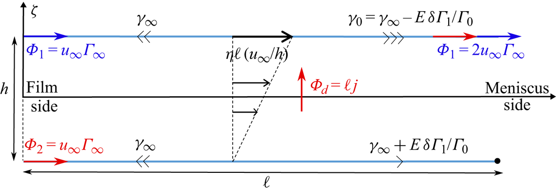
The key fact at the origin of the dissipation is the dead-end role played by the lateral side of the free meniscus. In the top left film in figure 13, for example, the top interface can slide over the meniscus and be transferred to the central film, whereas the lateral one encounters the interface coming from the bottom left peripheral film. The meniscus cannot instantaneously absorb the surfactant flux and the lateral interface must slow down when reaching the meniscus. This breaks the symmetry between both interfaces and shears the film.
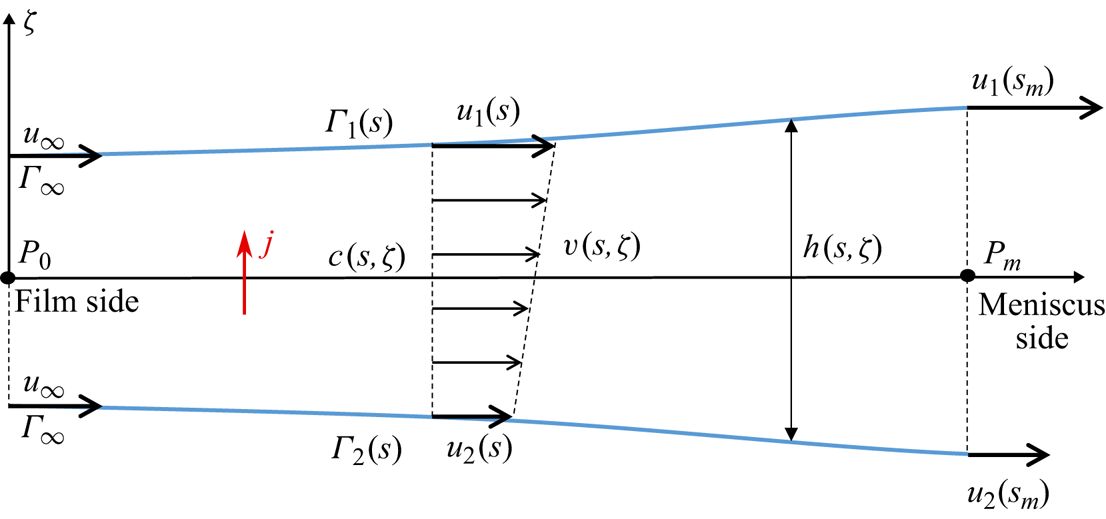
The model quantifies this mechanism by solving the coupled Stokes and surfactant transport equations in the appropriate limits. With this aim, we consider the piece of peripheral film shown in figure 14. The abscissa  $s$ and the film tangent
 ${\hat {\boldsymbol {t}}}$ are oriented from the peripheral film to the free meniscus, and the indices 1 and 2 indicate, respectively, the interface connected to the central film and the interface connected to the other peripheral film. The normal to the film is
 ${\hat {\boldsymbol {n}}}$, oriented from the interface 2 to the interface 1 and the corresponding variable is
 $\zeta$, with an origin in the middle of the film. The film thickness is
 $h(s)$, the bulk velocity is
 $v(s,\zeta ) {\hat {\boldsymbol {t}}}$, the interface velocities are
 $u_1(s)$ and
 $u_2(s)$ and the surface coverages are
 $\varGamma _1(s)$ and
 $\varGamma _2(s)$. The notation
 $\partial _x$ indicates the partial derivative with respect to any variable
 $x$.
Scheme of the sheared film (domain C in figure 13) and notations used in the text. The peripheral film is on the left side of the figure ( $s<0$) and the free meniscus on the right side (
 $s>s_m$). The interface (2) is connected to the interface of the symmetric peripheral film, whereas the interface (1) is connected to the central film. The case
 $u_\infty >0$ represented here corresponds to the compression case.

For the sake of simplicity, and in an attempt to build a relationship between the transfer velocity and the film tension at a given time, independently of the film history, we assume that the liquid and surfactant transports are stationary. This requires that the transient regime is shorter than the experimental time scale.
We start from the lubrication theory and neglect the Laplace pressure. The velocity field is therefore governed by  $\partial _{\zeta \zeta } v=0$, and the velocity profile is equal to, with
 $u_m=(u_1+u_2)/2$ and
 $\varDelta ^{f} u= u_1-u_2$
 \begin{equation} v(s,\zeta)=\frac{\varDelta^{f} u}{h} \zeta +u_m .\end{equation}
The flow rate at the position  $s$ is
 \begin{equation} Q=\int_{{-}h/2}^{h/2} v \, {\textrm{d}} \zeta=u_m h, \end{equation}
and, from the mass conservation, we find
 \begin{equation} h_{\infty}u_\infty=\frac{h}{2}(u_1+u_2), \end{equation}
with  $h_{\infty }$ and
 $u_\infty$ the thickness and velocity in the central part of the peripheral film, where both interfaces are identical.
The shear flow in the film imposes a viscous stress at the interface, coupled to a surface tension gradient by the Marangoni law
 \begin{equation} \eta\frac{\varDelta^{f} u}{h}=\partial_s\gamma_1 \quad \mbox{and} \quad \partial_s\gamma_2={-}\partial_s\gamma_1.\end{equation}
The surface tension is related to surface coverage  $\varGamma$ using (2.2) leading to
 \begin{equation} -\frac{E}{\varGamma_0} \partial_s\varGamma_1=\eta\frac{\varDelta^{f} u}{h} \quad \mbox{and} \quad \partial_s\varGamma_2={-}\partial_s\varGamma_1.\end{equation}
As already discussed in § 5.2, surfactant diffusion along the film is slower than the convection, and surfactant diffusion across the film is faster than the convection. The convection diffusion equation thus simplifies into  $\partial _{\zeta \zeta }c = 0$. We assume a fast adsorption process (no adsorption barrier) so that the equilibrium relation between the interface and the bulk, (2.3), can be used. The boundary conditions at the interfaces are thus
 $c_i=c_0+(\varGamma _i-\varGamma _0)/h_\varGamma$ (with
 $i=1$ or 2) and the bulk concentration is
 \begin{equation} c(s,\zeta)=c_0+\frac{\varGamma_1-\varGamma_2}{h h_{\varGamma}} \zeta +\frac{\varGamma_1+\varGamma_2}{2 h_{\varGamma}}-\frac{\varGamma_0}{h_\varGamma}. \end{equation}
Using this profile and neglecting surface diffusion, the surfactant conservation on each interface gives, with  $j$ the diffusive flux coming from the bulk to interface 1,
 $$\begin{gather} \partial_s(\varGamma_1 u_1)=j={-}D\frac{\varGamma_1-\varGamma_2}{hh_{\varGamma}}, \end{gather}$$
 $$\begin{gather}\partial_s(\varGamma_1 u_1)={-}\partial_s(\varGamma_2 u_2). \end{gather}$$
Equations (7.5b) and (7.8) imply that the two quantities  $\varGamma _1+\varGamma _2$ and
 $\varGamma _1u_1+\varGamma _2u_2$ are conserved along the film so
 $$\begin{gather} \varGamma_1+\varGamma_2=2 \varGamma_{\infty} , \end{gather}$$
 $$\begin{gather}\varGamma_1u_1+\varGamma_2u_2=2 \varGamma_{\infty}u_\infty , \end{gather}$$
leading to
 $$\begin{gather} \varGamma_2=2 \varGamma_{\infty}-\varGamma_1 , \end{gather}$$
 $$\begin{gather}u_2=\frac{2 \varGamma_{\infty}u_{\infty}}{2 \varGamma_{\infty}-\varGamma_1}-\frac{u_1\varGamma_1}{2\varGamma_{\infty} -\varGamma_1}. \end{gather}$$
The whole dynamics is finally controlled by a set of two coupled differential equations, deduced respectively from the Marangoni law and from the surfactant mass balance at interface 1
 $$\begin{gather} \partial_s \varGamma_1={-}\frac{\eta\varGamma_0}{E} \frac{\varDelta^{f} u}{h}, \end{gather}$$
 $$\begin{gather}\partial_s(\varGamma_1 u_1)={-}2D\frac{\varGamma_1- \varGamma_{\infty}}{hh_{\varGamma}}, \end{gather}$$
where
 $$\begin{gather} \varDelta^{f} u=u_1-u_2 =(u_1-u_{\infty})\frac{2\varGamma_{\infty}}{2\varGamma_{\infty}- \varGamma_1} , \end{gather}$$
 $$\begin{gather}h=\frac{2h_{\infty}u_{\infty}}{u_1+u_2} =\frac{h_{\infty}u_{\infty}(2\varGamma_{\infty}- \varGamma_1)}{\varGamma_{\infty}u_{\infty} +u_1(\varGamma_{\infty}-\varGamma_1)} . \end{gather}$$
7.2. Boundary conditions
The model applies only in the sheared film defined in § 6.2 and depicted as the domain C in figure 13. The problem is thus solved between the point  $P_0$, chosen as the abscissa origin
 $s=0$, at the boundary between this domain and the central part of the peripheral film (domain D), and the point
 $P_m$ at
 $s=s_m$ at its boundary with the dynamical meniscus (domain B).
By definition, the conditions at  $s<0$ are
 $u_1 = u_{\infty }$ and
 $\varGamma _1= \varGamma _{\infty }$ imposed in the central part of the peripheral film (see figure 14). If the peripheral film is compressed
 $\varGamma _{\infty } > \varGamma _0$ and
 $u_{\infty }>0$; the signs are opposite if the film is stretched.
These boundary conditions are sufficient to solve the system ((7.13) and (7.14)). However, the aim of the solution is to determine the relationship between the surface coverage  $\varGamma _{\infty }$ (related to the tension in the peripheral film) and the film velocity
 $u_\infty$ (related to its transfer velocity). In the following,
 $\varGamma _{\infty }$ will thus be considered as our control parameter, and
 $u_\infty$ as an unknown quantity. As expected, the problem should thus be closed with additional conditions, at the meniscus. These conditions quantify the dead-end role of the meniscus for the interface 2 and thus provides the sought relationship between
 $u_\infty$ and
 $\varGamma _{\infty }$.
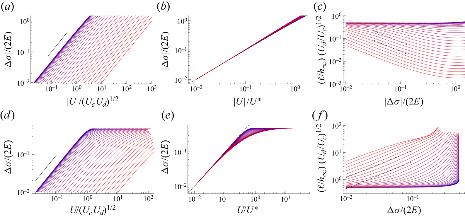
For large values of  $s$, the meniscus is reached and the assumption of vanishing Laplace pressure fails. The boundary conditions must therefore be imposed at the boundary
 $P_m$ shown in figure 14, where the used approximations are satisfied, and not in the central film (for interface 1) nor in the symmetry plane
 $z=0$ (for interface 2, at the point
 $P_s$ of the meniscus lateral interface shown in figure 13). We thus need to make additional assumptions.
For interface 1, the tension in the central film is the equilibrium tension, and does not vary much along the static meniscus interface, nor along the dynamical meniscus interface, as shown in §§ 6.3 and 6.4. We therefore impose the condition  $\varGamma _1(s_m) = \varGamma _0$, which determines
 $s_m$.
On interface 2, the velocity vanishes at the point  $P_s$ by symmetry. This information must be used to build the condition at the required point
 $P_m$. The surfactant mass balance made on the piece of interface between
 $P_m$ and
 $P_s$ imposes
 \begin{equation} \varGamma_2(s_m) u_2(s_m) + j_m = 0 , \end{equation}
with  $j_m$ the amount of surfactant adsorbed from the bulk along the meniscus interface, per unit time, between
 $P_m$ and
 $P_s$. This quantity is difficult to predict and its modelling would require a better control of the solution transport along the axis of the meniscus (i.e. in the
 $y$ direction). In our model, we use the simplest phenomenological relationship
 \begin{equation} j_m ={-} \frac{r_m}{\tau} ( \varGamma_2(s_m) - \varGamma_0 ), \end{equation}
with  $\tau$ the characteristic adsorption time of the surfactants, from the meniscus bulk at the reference concentration
 $c_0$ to the interface 2 at a concentration
 $\varGamma _2(s_m)$. For a purely diffusive case, this flux would be
 $j_m= - r_m D (\varGamma _2(s_m) - \varGamma _{0})/(h_\varGamma \ell _{mbl})$, with
 $\ell _{mbl} \sim \sqrt {D t}$ the thickness of the mass boundary layer, of the order of 10
 $\mathrm {\mu }$m after one second. This leads to
 $\tau _{diff} \sim h_\varGamma \ell _{mbl} / D \sim h_\varGamma \sqrt {t/D} \sim 1$ s and
 $U_m^{diff}=r_m/\tau ^{diff} \sim 5 \times 10^{-4}$ m s
 $^{-1}$. However, convection and recirculation are important in the meniscus, and a faster transport can a priori be achieved. The comparison with the experimental results of figure 19 will evidence a posteriori that
 $U_m = r_m/\tau$ evolves during the dynamical process. It is larger than
 $U^{diff}$ at short time and becomes negligible afterwards.
The boundary condition at  $s_m$ for the interface 2, which closes the model, is thus finally
 \begin{equation} \varGamma_2(s_m) u_2(s_m) = \frac{r_m}{\tau} ( \varGamma_2(s_m) - \varGamma_{0} ). \end{equation}
In order to perform a numerical solution, the asymptotic conditions  $u_1 = u_{\infty }$ and
 $\varGamma _1= \varGamma _{\infty }$ at
 $s \to - \infty$ need to be replaced by a condition at
 $s=0$. As shown below,
 $\varGamma _1$ converges exponentially to
 $\varGamma _{\infty }$ when
 $s \to -\infty$. We thus define the position origin
 $s=0$ as the point satisfying
 \begin{equation} \varGamma_1 (0) =\varGamma_{\infty} + \alpha ( \varGamma_0 - \varGamma_{\infty}) , \end{equation}
with  $\alpha$ a small parameter. The corresponding value
 $u_1(0)$ is determined in § 7.4.2 by linearization of the equation set. Numerically, the problem is solved with
 $\alpha =0.05$, without loss of generality. The length
 $s_m$, used in the numerical solution, then depends on the arbitrary choice of
 $\alpha$. To correctly characterize the sheared film length we therefore introduced the characteristic length
 $\ell$ extracted a posteriori from an exponential fit of the numerical solution.
The system ((7.13) and (7.14)), with the boundary conditions both in the thin film and in the meniscus constitutes a closed problem, with  $\varGamma _\infty$,
 $h_\infty$ and the physico-chemical constants as known parameters and
 $u_\infty$ and the length
 $s_m$ (or
 $\ell$) of the sheared film as solutions.
7.3. Scaling laws
Before performing the whole numerical solution, some scaling laws can be anticipated. In the following, we use the notation  $\delta$ for a difference
 $X(s_m)- X(0)$ for any variable
 $X$, in order to estimate the spatial derivative of
 $X$. In contrast the notation
 ${\rm \Delta}$ indicates a variation from the equilibrium value. Finally
 $\varDelta ^{f}$ indicates a difference between the interfaces 1 and 2 across the film, close to the meniscus. We thus define
 $\delta \varGamma _1 =\varGamma _1(s_m) - \varGamma _\infty = \varGamma _0 - \varGamma _\infty$ and
 $\delta u_1 = u_1(s_m) - u_\infty$. Note that (7.11) imposes that
 $\varGamma _1(s_m) - \varGamma _2(s_m) = 2 \delta \varGamma _1$ so the same scaling and the same sign hold for both
 $\delta \varGamma _1$ and
 $\varDelta ^{f} \varGamma$, representing respectively the concentration variation along the interface 1 and the concentration difference between both interfaces. Similarly, (7.15) imposes that
 $\varDelta ^{f} u$ between both interfaces is of the same order as
 $\delta u_1$, as long as
 $\delta \varGamma _1 \ll \varGamma _0$.
With these definitions, we have  $u_\infty >0$,
 $\delta \varGamma _1 <0$,
 $\delta u_1 > 0$ for the pushing case, and the opposite for the pulling case. The different scaling laws obtained below are built on three characteristic velocities, the capillary velocity
 $U_c$, the diffusion velocity
 $U_d$ and the reservoir velocity associated with the meniscus
 $U_m$ defined as
 \begin{equation} U_c=\frac{E}{\eta} , \quad U_d=\frac{D}{h_\varGamma} ,\quad U_m=\frac{r_m}{\tau}. \end{equation}
The orders of magnitude established in § 8 lead to  $U_c \sim 3$ m s
 $^{-1}$ and
 $U_d\sim 5 \times 10^{-7}$ m s
 $^{-1}$. The film thickness always remains close to its asymptotic value (see figure 16c). Scaling laws for
 $\ell$ and for
 $U= - u_1(s_m)$ (given our conventions these two velocities are defined with an opposite sign, see figure 14), are proposed below, in the three different regimes that we identified.
7.3.1. Vanishing flux at the meniscus
We first assume that the meniscus does not play any reservoir role, the flux  $j_m$ thus being negligible in (7.17). This limit, which can be reached either because of a vanishing velocity or because of a vanishing DOH surface excess at the meniscus on interface 2, is explored first in the compression case, and then in the stretching case.
In compression, the surface excess  $\varGamma _2(s_m)$ is larger than its equilibrium value and cannot vanish. It is, however, usually observed that the velocity may vanish in such cases, this effect being known as the stagnant cap limit (Cuenot, Magnaudet & Spennato Reference Cuenot, Magnaudet and Spennato1997; Cantat Reference Cantat2011; Reichert et al. Reference Reichert, Cantat and Jullien2019). In this limit, and in steady state, the whole flux
 $\varPhi _2= u_\infty \varGamma _\infty$ advected on interface 2 must diffuse to interface 1, which imposes
 $\varGamma _\infty u_\infty \sim \ell j \sim - D \ell \delta \varGamma _1 / (h_\infty h_\varGamma )$ (as depicted in figure 15). The length
 $\ell$ of the sheared film can thus be seen as an exchange length, which must be large enough for the whole flux
 $\varPhi _2$ to reach the interface 1 by diffusion, before reaching the stagnant cap at the meniscus. Then, on the interface 1, the flux at the meniscus must be twice the flux advected on the interface at the peripheral film side. As
 $\varGamma$ remains of the order of
 $\varGamma _0$, the velocity
 $u_1(s_m)$ is of the order of
 $2 u_\infty$ ((7.10)), which leads to
 $\delta u_1 \sim u_\infty$. The viscous force between both interfaces is thus of the order of
 $\eta u_\infty \ell /h$. A second coupling between the unknown quantities
 $\ell$ and
 $u_\infty$ is given by the Marangoni law
 $-E \delta \varGamma _1/\varGamma _\infty \sim \eta u_\infty \ell /h_\infty$.
Scheme of the dynamics in the limit of vanishing velocity at the meniscus on interface 2 (bottom interface). Interface 1 (top interface) is connected to the peripheral film (on the left) and to the central film (on the right) through the free meniscus. For the compression, the surfactant excess is lower in the central film than in the peripheral film, so  $\delta \varGamma _1 <0$ and
 $u_\infty >0$. The signs are opposite for the stretching. Surfactant fluxes initially coming from interfaces 1 and 2 are illustrated by the blue and red arrows, respectively. Black arrows illustrate the tension and the viscous forces.

Combining both relationships, we get the following scaling laws:
 $$\begin{gather} \frac{\delta \varGamma_1}{\varGamma_0}\sim{-}\frac{u_1(s_m)}{\sqrt{U_c U_d}}\mbox{ so } \frac{{\rm \Delta}\sigma}{2E} \sim \frac{U}{\sqrt{U_c U_d}}, \end{gather}$$
 $$\begin{gather}\ell \sim h_\infty \left(\frac{E h_\varGamma}{\eta D} \right)^{1/2} \sim h_\infty \sqrt{\frac{U_c}{U_d}} . \end{gather}$$
In this regime, the relevant velocity scale is  $\sqrt {U_c \, U_d} \sim 10^{-3}$ m s
 $^{-1}$. Using the experimental order of magnitude
 ${\rm \Delta} \sigma / E \sim 1$, the scaling (7.22) predicts a transfer velocity of the order of
 $10^{-3}$ m s
 $^{-1}$, as expected. The length
 $\ell$ of the sheared film is independent of the tension and its order of magnitude is
 $10^{3} h_\infty \sim 1$ mm. This validates the different assumptions made:
 $\ell \ll d$ ensuring that the film is not entirely sheared and
 $\ell \gg h_\infty$ ensuring that the lubrication approximation can be used. Moreover,
 $\ell > \ell _m \sim 100\ \mathrm {\mu }$m, the extension of the dynamical meniscus, so that Laplace is negligible in the sheared film. However, these two length scales may become similar for different solutions and the coupling between the sheared film and the dynamical meniscus should probably be considered in a more refined model.
In the stretching case, we need to consider two situations: the flux at the meniscus may vanish because (i) the velocity vanishes or because (ii) the concentration vanishes. In the limit of small tension in the film ( ${\rm \Delta} \sigma \ll E$), the surface excess satisfies the condition
 $\delta \varGamma _1 \ll \varGamma$, and only the first case needs to be considered. It leads to the same scaling as in the compression case: (7.22) and (7.23), with
 $\delta \varGamma _1 > 0$ and
 $u_1(s_m)< 0$.
However, at some critical tension, the surface excess vanishes on interface 2, at the meniscus, and the stretching dynamics strongly differs from the compression dynamics: the tension does not vary linearly with the transfer velocity anymore and saturates at an upper limit, whatever the value of the transfer velocity. From (7.11) we deduce, as the surface excess  $\varGamma _2(s_m)$ must remain positive, that this critical case occurs for
 $\varGamma _1 (s_m) = 2 \varGamma _\infty$, i.e.
 $\varGamma _\infty = 0.5 \varGamma _0$. This corresponds to
 ${\rm \Delta} \sigma /(2E)=0.5$, which constitutes an upper limit for this control parameter. From (5.5), the corresponding upper limit for the deformation is
 $\varepsilon ^{max} = 1$. The divergences associated with this particular regime are investigated in § 7.3.3.
In summary, when the meniscus cannot supply or adsorb any surfactant flux (small  $U_m$) the dynamics induced by a meniscus can be described by a well-defined constitutive law: the tension difference
 ${\rm \Delta} \sigma$ varies linearly with the transfer velocity; in the extension case, this tension saturates at
 ${\rm \Delta} \sigma =E$, and does not depend on the velocity at larger velocity values.
7.3.2. Fast meniscus transport
Here, we consider the limit  $U_m \gg \sqrt {U_c U_d}$, in which the meniscus plays the role of a reservoir for the surfactants and almost entirely absorbs (or provides in the stretching case) the flux
 $\varPhi = \varGamma _\infty u_\infty$ advected on the interface 2. In that case,
 $u_1(s_m) \sim u_2(s_m)$ and (7.19) directly provides the relationship between the velocity at the meniscus and the surface excess
 \begin{equation} u_1(s_m) \sim u_\infty \sim{-} \frac{\delta \varGamma_1}{\varGamma_0} U_m \mbox{ so } \frac{{\rm \Delta}\sigma}{2E} \sim \frac{U}{U_m} .\end{equation}
The scaling for  $\ell$ can be deduced from the flux conservation (7.14) leading to
 $u_\infty \delta \varGamma _1 + \varGamma _0 \delta u_1 \sim - \ell D \delta \varGamma _1 /(h_\infty h_\varGamma )$. Coupled to the Marangoni law
 $\eta \ell \delta u_1 / h_\infty \sim - E \delta \varGamma _1 /\varGamma _0$ it simplifies into
 \begin{equation} u_\infty - U_c \frac{h_\infty}{\ell} \sim{-} U_d \frac{\ell }{h_\infty}.\end{equation}
The various limits discussed below each corresponds to one of these three terms within (7.25) being negligible. The term  $u_\infty$ is the smallest in the limit
 $U_m |\delta \varGamma _1|/\varGamma _0 \ll \sqrt {U_c U_d}$. In that case, the scaling is the one of (7.23). The two other cases are discussed below, and depend on the sign of
 $u_\infty$. In the pushing case,
 $u_\infty$ is positive and can thus only balance
 $U_c h_\infty /\ell$. Physically, it means that the diffusive transport between both interfaces is negligible. This limit is consistent with the mechanical constraints because (i) the interface flows from the peripheral film at large surface excess to the central film at equilibrium coverage so
 $\delta \varGamma _1< 0$, (ii) on the other hand,
 $\delta u_1> 0$, leading to an increase of the area on interface 1, and thus a decrease of the surfactant excess
 $\varGamma _1$ along the sheared film. A consistent solution can thus be reached without any diffusion, the convection and the interface deformation providing the required Marangoni stress. The scaling obtained in the limit of large
 $U_m$, in compression, is thus
 \begin{equation} \ell \sim h_\infty \left( \frac{-\delta \varGamma_1}{\varGamma_\infty} \right)^{{-}1} \frac{U_c}{U_m} . \end{equation}
The length  $\ell$ diverges at small
 $\delta \varGamma _1$, which may seem surprising. However, in this limit the velocity difference between both interfaces decreases, and the shear, even if spread over a large part of the film, is very small.
The dynamics is entirely different in the stretching case, as both terms of the left-hand side of (7.25) have the same sign. Indeed, as  $|u_\infty | < |u_1(s_m)|$, the interface 1 is surprisingly compressed during its transport through the sheared film. However, the positive tension associated with the film stretching imposes
 $\delta \varGamma _1 > 0$. This can only be achieved with a non-negligible diffusion from the interface 2. In the limit
 $U_m \gg \sqrt {U_c U_d}$, the obtained scaling for the stretching case is
 \begin{equation} \ell \sim h_\infty \frac{\delta \varGamma_1}{\varGamma_\infty} \frac{U_m}{U_d}, \end{equation}
whereas the scaling of (7.23) is recovered in the other limit.
It should be noted that  $\ell$ becomes large for large
 $U_m$. As for the small
 $\delta \varGamma _1$ limit in compression, the velocity difference between both interfaces decreases and the dissipation induced by the meniscus frustration becomes negligible.
In this second regime, governed by the meniscus, the tension difference increases linearly with the transfer velocity, with a prefactor  $2 E/ U_m$. As in this regime
 $U_m \gg \sqrt {U_c U_d}$, this prefactor is smaller than the prefactor
 $2 E/ \sqrt {U_c U_d}$ obtained in the first regime (see (7.22)). The meniscus acts as a reservoir for the surfactants, and attenuates the film shear. A strong asymmetry arises for the exchange lengths: in the compression case, the surface excess gradients establish on each interface with a negligible diffusion from one interface to the other, and the sheared film length vanishes at large
 $U_m$. In contrast, these gradients require a large exchange between interfaces in the stretching case, and
 $\ell$ increases with
 $U_m$.
7.3.3. Diverging behaviour in the stretching case
In this last regime, observed at large  $\delta \varGamma _1$, the tension in the stretched film becomes independent of the velocity and saturates at
 ${\rm \Delta} \sigma = E$. The assumption
 $\delta \varGamma _1 \ll \varGamma _0$ used in the previous section is not valid anymore and a different scaling applies.
We define  $\varGamma _\infty = (\varGamma _0/2) (1 +\hat {\varepsilon })$, with
 $\hat {\varepsilon }$ a small parameter, so that the concentration at the meniscus is
 $\varGamma _2(s_m)/\varGamma _0 = \hat {\varepsilon }$. At large
 $U_m$, the velocities in the stretched film are much higher than their gradients and
 $u_2(s_m) \sim u_\infty$. The condition (7.19) thus becomes
 \begin{equation} u_\infty \sim{-} \frac{U_m}{\hat{\varepsilon}}.\end{equation}
The sheared film extension is obtained from (7.25), in which the term proportional to  $U_c$ can be neglected. This leads to
 \begin{equation} \ell \sim \frac{h_\infty}{\hat{\varepsilon}} \frac{U_m}{U_d}.\end{equation}
All the scalings obtained in this section are obtained numerically in the following section.
7.4. Numerical solution
7.4.1. Non-dimensionalization
In order to reduce the number of parameters to explore, we now build a dimensionless form of the problem using  $u_1=|u_\infty |\bar {u}$,
 $\varGamma _1=\varGamma _{\infty }\bar {\varGamma }$,
 $h=h_{\infty }\bar {h}$ and
 $s=({Eh_{\infty }}/{\eta |u_\infty |})\bar {s}$. The scaling chosen for
 $s$ comes form (7.13). In the dimensionless form, and combining (7.13) and (7.14), the new system writes
 $$\begin{gather} \partial_{\bar{s}}\bar{\varGamma}={-}\frac{1}{\chi_{\infty}}\frac{\varDelta^{f} \bar{u}}{\bar{h}} , \end{gather}$$
 $$\begin{gather}\partial_{\bar{s}}\bar{u}=\frac{1}{\chi_{\infty}}\frac{\bar{u}\varDelta^{f} \bar{u}}{\bar{\varGamma}\bar{h}}-2 A \frac{\bar{\varGamma}-1}{\bar{\varGamma}\bar{h}} , \end{gather}$$
with  $\chi _{\infty }=\varGamma _{\infty }/\varGamma _0$,
 $A=DE/(\eta u_\infty ^{2}h_{\varGamma })= U_c U_d / u_\infty ^{2}$ and
 $$\begin{gather} \varDelta^{f} \bar{u}=\frac{2}{2-\bar{\varGamma}} ( \bar{u} - \bar{u}_\infty ) , \end{gather}$$
 $$\begin{gather}\bar{h}=\bar{u}_\infty \frac{2-\bar{\varGamma}}{\bar{u}_\infty+ \bar{u}(1-\bar{\varGamma})}. \end{gather}$$
The asymptotic velocity in the film at small  $s$ is
 $\bar {u}_\infty =1$ if the film is pushed toward the meniscus; in that case, the condition
 $\chi _\infty >1$ must be fulfilled to ensure the existence of solutions. If the film is pulled, we have
 $\bar {u}_\infty =-1$ and
 $\chi _\infty <1$. In both cases the asymptotic concentration in the film is
 $\bar {\varGamma } = 1$. Note that
 $A$, more precisely
 $1/\sqrt {A}$, is a dimensionless velocity comparing the peripheral film velocity
 $u_\infty$ and the intrinsic physico-chemical velocity
 $\sqrt {U_cU_d}$ as identify in § 7.3.1.
The conditions at the meniscus become
 $$\begin{gather} \bar{\varGamma}(\bar{s}_m) = \frac{1}{\chi_\infty} , \end{gather}$$
 $$\begin{gather}( \bar{u} - \varDelta^{f}\bar{u})(\bar{s}_m) = K \sqrt{A} \frac{\chi_\infty -1}{2\chi_\infty -1} , \end{gather}$$
with
 \begin{equation} K= \frac{2 r_m}{\tau}\sqrt{\frac{\eta h_\varGamma}{DE}} = \frac{ 2 U_m}{\sqrt{U_c U_d}} , \end{equation}
which compares the reservoir velocity to the physico-chemical velocity. For  $K \gg 1$ meniscus behaves as a reservoir as analysed in the fast meniscus transport case in § 7.3.2 while for
 $K\ll 1$ the dynamics is governed by the physico-chemical process as described in § 7.3.1.
Equations (7.30) and (7.31) are dimensionless analogues of the system (7.13) and (7.14) and (7.34) and (7.35) are the dimensionless boundary condition defined in (7.19) and (7.20). Finally, the limit discussed in § 7.3.3 is obtained in the stretching case, for  $\chi _\infty \to 1/2$.
7.4.2. Linearization and boundary conditions at  $\bar {s}=0$

To solve the system (7.30) and (7.31), one needs to impose compatible boundary conditions at  $\bar {s}=0$, which we obtain by linearizing the equations. We introduce
 $\bar {u}=\bar {u}_\infty +\varepsilon _u$ and
 $\bar {\varGamma }=1+\varepsilon _\varGamma$ with
 $\varepsilon _u,\varepsilon _\varGamma \ll 1$. At first order in these small parameters, we get
 $\varDelta ^{f} \bar {u}= 2 \varepsilon _u$,
 $\bar {h}=1$,
 $\partial _{\bar {s}} \varepsilon _\varGamma =- ({2}/{\chi _{\infty }})\varepsilon _u$ and
 $\partial _{\bar {s}}\varepsilon _u=({2 \bar {u}_\infty }/{\chi _{\infty }})\varepsilon _u - 2A\varepsilon _\varGamma$, having the solutions
 $\varepsilon _\varGamma =a_\varGamma {e}^{ks}$ and
 $\varepsilon _u=a_u {e}^{ks}$. Using the convention chosen in (7.20) to define the origin of
 $s$, this imposes
 $a_\varGamma =\alpha (1 - \chi _\infty )/\chi _\infty$ where
 $\alpha =0.05$ is a small arbitrary constant involved in the numerical solution. Injecting these solutions in the linearized equations gives
 $$\begin{gather} a_\varGamma k + a_u \frac{2}{\chi_{\infty}} = 0 , \end{gather}$$
 $$\begin{gather}2 A a_\varGamma + a_u \left(k -\frac{2 \bar{u}_\infty}{\chi_{\infty}} \right) = 0 , \end{gather}$$
which characteristic equation is
 \begin{equation} k^{2} - 2\frac{\bar{u}_\infty}{\chi_{\infty}}k-\frac{4A}{\chi_{\infty}}=0 . \end{equation}
Since  $A>0$,
 $\chi _{\infty }>0$ and
 $\bar {u}_\infty = 1$ for the pushing case and
 $\bar {u}_\infty = -1$ for the pulling case, the only positive solution, compatible with the asymptotic behaviour at
 $s \to - \infty$, is in both cases
 \begin{equation} k=\frac{1}{\chi_{\infty}}(\sqrt{1+4A\chi_{\infty}}+ \bar{u}_\infty), \end{equation}
leading to the initial conditions
 $$\begin{gather} \bar{\varGamma}(0)=1+ \alpha \frac{1 - \chi_\infty}{\chi_\infty}, \end{gather}$$
 $$\begin{gather}\bar{u}(0)=\bar{u}_\infty - \alpha \frac{1 - \chi_\infty}{2 \chi_\infty} (\sqrt{1+4A\chi_{\infty}}+ \bar{u}_\infty ). \end{gather}$$
7.4.3. Definition of the relevant numerical quantities
The nonlinear coupled equations (7.30) and (7.31) are first solved with the Matlab solver ode45 with the initial conditions (7.41), (7.42), for a given value of  $\chi _\infty$,
 $K$ and
 $A$. The upper
 $s$ value
 $s_m$ is determined with (7.34). This solution is performed with different values of the parameter
 $A$ until the condition (7.35) is satisfied too, for the specific value
 $A^{*}( K,\chi _{\infty })$. The obtained parameter
 $A^{*}(K,\chi _\infty )$ eventually provides the film velocity as a function of its asymptotic film tension, by simply using the definition of
 $A$ in (7.31)
 \begin{equation} |u_\infty| = \frac{\sqrt{U_c U_d}}{\sqrt{A^{*}(K,\varGamma_\infty/\varGamma_{eq})}} . \end{equation}
Note that the sign of  $u_\infty$ must be prescribed a priori, as
 $\bar {u}$ reaches
 $\bar {u}_\infty = \pm 1$, in the pushing and pulling cases respectively, at large negative
 $s$. Figure 16 shows the typical spatial evolution in the sheared domain of the surface coverages, velocities of both interfaces and of the film thicknesses for both the extension and compression cases.
Evolution of the dimensionless surface concentrations (a), surface velocities (b) and film thicknesses (c) in terms of the dimensionless coordinate ( $s/h_{\infty }\sqrt {U_d/U_c}$) for
 $|\delta \varGamma |/\varGamma _0=0.2$ and
 $K=10^{-3}$ (solid lines) and
 $K=0.39$ (dashed lines). The extension case is represented in blue and the compression in red. The curves stop at different
 $s=s_m$ since
 $s_m$ depends on
 $K$ and
 $\delta \varGamma$. The
 $K=10^{-3}$ example is representative of the small
 $K$ regime discussed in § 7.3.1, whereas the
 $K=0.39$ case is a generic example, in which all effects compete.

From  $A^{*}(K,\chi _\infty )$ we can now predict the quantities experimentally measured in figure 12. The film tension difference
 ${\rm \Delta} \sigma$ between the peripheral film and the central film can be expressed as a function of the Gibbs elasticity and the numerical parameter
 $\chi _\infty$ with the relation
 \begin{equation} \frac{{\rm \Delta} \sigma}{2 E}=\frac{\delta \varGamma_1}{\varGamma_0}= 1 - \chi_\infty . \end{equation}
The velocity in the central film  $U$, defined as negative for the compression and positive for the extension, is identified with
 $-u_1(s_m)$, the velocity being assumed to be constant along the meniscus side (on interface 1). This velocity is thus expressed as
 \begin{equation} \frac{U}{\sqrt{U_c U_d}} ={-}\frac{ |u_\infty|}{\sqrt{U_c U_d}} \bar{u}_1(\bar{s}_m) ={-} \frac{\bar{u}_1(\bar{s}_m)}{\sqrt{A^{*}}} . \end{equation}
The other significant dynamical quantity is the length  $\ell$ of the sheared film. Its non-dimensional value
 $\bar {\ell }$ is obtained by fitting the evolution of
 $\bar {\varGamma }(\bar {s})$ with an exponential function. Then we get
 \begin{equation} \frac{\ell}{h_\infty}\sqrt{\frac{U_d}{U_c}}=\frac{\bar{\ell} h_\infty U_c}{h_\infty |u_\infty|}\sqrt{\frac{U_d}{U_c}}=\bar{\ell}\sqrt{A^{*}} . \end{equation}
7.4.4. Numerical results
The numerical results for compression and extension are shown in figure 17. The relationship between the tension difference and the transfer velocity is shown in (a) for the compression. For all the values of the parameter  $K= 2 U_m/\sqrt {U_c U_d}$ the tension is proportional to the velocity. As expected from the scaling laws analysis, the prefactor is constant at small
 $K$ ((7.22)) and decreases with
 $K$ at large
 $K$ ((7.24)). As shown in figure 17(b), all numerical data fall on a single master curve
 \begin{equation} \frac{{\rm \Delta} \sigma}{2 E } = \frac{U}{U^{*}},\end{equation}
if the velocity is rescaled by
 \begin{equation} U^{*} = \sqrt{U_c U_d} (2+ K)= 2 (\sqrt{U_c U_d} + U_m),\end{equation}
which nicely interpolates between the asymptotic behaviours at small and large  $K$. This is the sought constitutive relation for the meniscus, based on the microscopic physico-chemical properties of the system. This prediction nevertheless relies on the linearized (2.2), which fails at large compression, as will be discussed in § 8.6.
Numerical solutions for the compression (top) and the extension (bottom). The control parameter  $K= 2 U_m/\sqrt {U_c U_d}$ has been varied logarithmically from
 $10^{-3}$(blue curves) to
 $10^{3}$ (red curves). (a), (d) Film tension difference
 ${\rm \Delta} \sigma$ between the peripheral film and the central film, rescaled by the film elasticity
 $2 E$, as a function of the transfer velocity
 $U$ in the central film, rescaled by
 $\sqrt {U_c U_d}$. The slope of the black lines corresponds to a linear law. For the compression,
 ${\rm \Delta} \sigma$ and
 $U$ are negative and we plotted their absolute values. (b), (e) Same data, with the velocity rescaled by
 $U^{*} = 2.0 \sqrt (U_d U_c) + 2.0 \times U_m$, which provides the best fit of the numerical data and smoothly interpolates between the scalings 7.22 and 7.24. The dashed line corresponds to
 ${\rm \Delta} \sigma /(2 E)= U/U^{*}$ and the horizontal dashed line in (e) is
 ${\rm \Delta} \sigma /(2 E)= 0.5$. (c), (f) Length
 $\ell$ of the sheared film, rescaled by
 $h_\infty \sqrt {U_c/U_d}$, as a function of the tension rescaled by
 $2 E$. The black dashed lines in (c) corresponds to
 $\ell /(h_\infty \sqrt {U_c/U_d})= 0.57 /( K {\rm \Delta} \sigma /(2 E))$, for two values of
 $K$, corresponding to the closest curve (
 $K = 81$ and
 $208$). This is the scaling of (7.26), with a fitted prefactor. Similarly, in (f) they correspond to
 $\ell /(h_\infty \sqrt {U_c/U_d})= 0.57 K {\rm \Delta} \sigma /(2 E)$, for the same
 $K$ values (scaling of (7.27)).

The same behaviour is recovered for the extension case (figure 17d,e) at small tension. The master curve of (7.47) is still obtained, which is consistent with a linear relationship between  $U$ and
 ${\rm \Delta} \sigma$, expected in the limit of vanishing
 ${\rm \Delta} \sigma$. However, at larger tension, the saturation at
 ${\rm \Delta} \sigma /(2 E) = 0.5$ breaks the symmetry between stretching and compression. It corresponds to a vanishing interface concentration at the meniscus, on the lateral side (interface 2). The tension reaches a plateau and the velocity diverges, as discussed in § 7.3.3 and in Appendix E.
The sheared film length  $\ell$ is plotted in figure 17(c) as a function of the film tension difference for the compression case. It is independent of the tension at small
 $K$ value and it decreases with
 ${\rm \Delta} \sigma$ at large
 $K$, as expected from (7.23) and (7.26). Its upper bound is
 $h_\infty \sqrt {U_c/U_d} \sim 10^{-3}$ m, much smaller than the film size, as a priori assumed by the model. At large
 $U_m$,
 $\ell$ can becomes of the order of the dynamical meniscus length
 $\ell _m$. In that case, some corrections related to the Laplace pressure are expected in the sheared film domain. Finally, for significant tension variations the length reaches another constant value, which depends on
 $U_m$ and is not captured by our scaling analysis.
For the extension case, figure 17(f), the sheared length at small  $K$ (
 $2 U_m \ll \sqrt {U_c U_d}$) is constant and is the same as in compression. A significant difference with the compression appears at large
 $K$ where
 $\ell$ increases with
 ${\rm \Delta} \sigma$ as predicted by (7.27). Moreover, the sheared length diverges close the tension saturation
 ${\rm \Delta} \sigma /(2E)=0.5$ with a scaling law predicted in (7.29) and verified in Appendix E. When
 $\ell$ becomes significant, the sheared film invades the entire peripheral film and our model breaks down as the domain D represented in figure 13 entirely disappears.
On the basis of these numerical results, we can now refine our description of the transfer velocity. Its value  $U$ is defined here as the velocity of the central part of the central film. The velocity
 $U_p$ of the central part of the peripheral films has been assumed to be close to
 $U$ in § 3.1, on the basis of the observations reported in Bussonnière et al. (Reference Bussonnière, Shabalina, Ah-Thon, Le Fur and Cantat2020). The corresponding numerical quantities are
 $U= - u_1(s_m)$ and
 $U_p= - u_\infty$, which actually differ from each other. Indeed, using (7.11) and (7.19) at
 $s=s_m$ we get
 \begin{equation} u_2(s_m)= 2 U_m \frac{\varGamma_\infty - \varGamma_0}{2 \varGamma_\infty - \varGamma_0} , \end{equation}
so from (7.12) and (7.47) we deduce
 \begin{equation} U = \frac{-2 u_\infty}{1+ 2\dfrac{U_m}{U^{*}} - 2 \dfrac{u_\infty}{U^{*}} } =U_p \frac{ 2 \sqrt{U_c U_d} + 2 U_m}{U_p + \sqrt{U_c U_d} + 2 U_m } . \end{equation}
At small tension ( $U$ and
 $U_p$ much smaller than
 $U^{*}$), we thus find
 $U \sim 2 U_p$ if
 $U_m \ll \sqrt {U_c\, U_d}$ and
 $U \sim U_p$ in the opposite limit. Physically, if
 $2 U_m \ll \sqrt {U_c U_d}$, the top interface, sliding at velocity
 $U$ toward the central film, must carry the total flux coming from both interfaces of the peripheral film. At small tension, the flux variations along the interfaces are only due to velocity variations and not to surface excess variations (see § 7.3.1), so
 $U\sim 2 U_p$. In contrast, in the case
 $2 U_m \gg \sqrt {U_c U_d}$, the flux on the external interface of the peripheral film is entirely absorbed/provided by the meniscus, and the top interface carries the same flux all along the sheared zone, so
 $U\sim U_p$. Note that figure 4 of Bussonnière et al. (Reference Bussonnière, Shabalina, Ah-Thon, Le Fur and Cantat2020) shows that both velocities
 $U$ and
 $U_p$ are of comparable value but does not allow us to make a quantitative comparison.
8. Comparison with experimental data
In this section, all the experiments performed at different deformation amplitudes ( ${\rm \Delta} d$), motor velocity (
 $V$) and mean position (
 $d_m$) are compared to the model developed in the previous section.
8.1. Compared quantities
The model developed in § 7 predicts the tension field on both interfaces in the sheared film, i.e. in the domain C of the figure 18. The film tension difference  ${\rm \Delta} \sigma$ (=
 $2{\rm \Delta} \gamma _s$) discussed in this section is thus only the film tension difference between the central part of the peripheral film and its boundary with the dynamical meniscus. It represents the dominant contribution to the film tension difference between the peripheral film and the central film. However, the tension jump in the dynamical meniscus, associated with the film extraction, is not entirely negligible and will be added as a correction. As shown in figure 18, this correction
 ${\rm \Delta} \gamma ^{out}$ is located in the peripheral film for the stretched side, and in the central film for the compressed side. Its value is given by (6.6) (Mysels et al. Reference Mysels, Shinoda and Frankel1959).
Localization of the different surface tension gradient in the experiments. Here, the symbol  ${\rm \Delta}$ corresponds to the difference between the two ends of the associated arrows;
 ${\rm \Delta} \gamma _\pm ^{out}$ are the tension differences induced by the Frankel film extraction (domain B, (6.6));
 ${\rm \Delta} \gamma _s^{\pm }=\frac {1}{2}{\rm \Delta} \sigma ^{\pm }$ are the tension differences predicted in § 7 for the sheared film (domain C). The transfer velocity
 $U$ is by convention positive on the stretched side and negative on the compressed side.

Following the scheme of the surface tension distribution along the interfaces (figure 18), we get the full theoretical prediction for the tension in the compressed film as
 \begin{equation} \frac{{\rm \Delta}\sigma_{th}^{-}}{2E}=\frac{2\gamma^{-}-2\gamma_0}{2E}= \frac{2{\rm \Delta}\gamma_s^{-}-2{\rm \Delta}\gamma_-^{out}}{2E}= \frac{{\rm \Delta}\sigma^{-}}{2E}-3.84\frac{\gamma_0}{E}\left(\frac{\eta |U|}{\gamma_0}\right)^{2/3},\end{equation}
with  ${\rm \Delta} \sigma ^{-}$ the film tension associated with the sheared film and predicted as a function of
 $U= -u_1 (s_m)$ by the model of § 7 (see figure 17). It should be noted that the tension of the meniscus interface connected to the central film is
 $\gamma _{mc}^{-}=\gamma _0-{\rm \Delta} \gamma ^{out}$ as shown in figure 18, and thus differs from the boundary condition
 $\gamma _0$ imposed in the shear model. However, this correction would only provide a second-order correction while greatly complicating the numerical solution.
The extension case is similar, but the tension jumps associated with the Frankel film extractions are located in the peripheral films. The extraction velocity is thus not identical on both interfaces: it is  $U= - u_1(s_m)$ on the top interface of the stretched film, and
 $U_2^{+} = -u_2(s_m)$, on the external interface (figure 18). In that case, we show in Appendix D that (6.6) remains valid if the averaged velocity is used.
The total film tension difference is finally given by
 \begin{equation} \frac{{\rm \Delta}\sigma_{th}^{+}}{2E}=\frac{2\gamma^{+}-2\gamma_0}{2E}= \frac{2{\rm \Delta}\gamma_s^{+}+2{\rm \Delta}\gamma_+^{out}}{2E}= \frac{{\rm \Delta}\sigma^{+}}{2E}+3.84\frac{\gamma_0}{E} \left(\frac{\eta (U+U_2^{+})}{2\gamma_0}\right)^{2/3} ,\end{equation}
with  ${\rm \Delta} \sigma ^{+}$ the film tension associated with the sheared film.
Note that, in both cases, the absolute value of  ${\rm \Delta} \sigma$ is increased by the additional term.
8.2. Time evolution and fitting procedure
The data associated with the experiments of the first campaign are plotted in figure 19. The time resolution of this campaign is not good enough to compute the transfer velocity  $U$ during the motor motion and only the relaxation phase (i.e. after the motors stop) is shown. A good reproducibility is observed for each set of parameters (each colour) but the relationship between
 ${\rm \Delta} \sigma$ and
 $U$ differs from one parameter value to the other, especially when
 ${\rm \Delta} d$ and
 $d_m$ vary, at early time (i.e. for large velocities). Moreover, at early time, experiments with injection consistently exhibit higher transfer velocities than the ones without injection which suggest that the velocity
 $U_m$ plays an important role in this regime. At later time, i.e. for smaller velocity, all the experiments remarkably converge toward a single master curve.
Comparison between the experimental and the theoretical viscous responses of an elementary foam. The solid lines and dashed lines are the predictions of (8.1) and (8.2), based on the numerical results shown in figure 17, with  $U_c = 3$ m s
 $^{-1}$,
 $U_d=5 \times 10^{-7}$ m s
 $^{-1}$ and, respectively
 $U_m\rightarrow 0$ mm s
 $^{-1}$ and
 $U_m=3$ mm s
 $^{-1}$. Experimental points correspond to the relaxation phase only (after the motor stops) and the large velocities thus correspond to the small times. Three control parameters were independently varied: the amplitude
 ${\rm \Delta} d$ in (a,d) with
 $d_m=12$ mm and
 $V=50$ mm s
 $^{-1}$; the motor velocity
 $V$ in (b,e) with
 ${\rm \Delta} d=6$ mm and
 $d_m=12$ mm; and the mean position
 $d_m$ in (c,f) with
 ${\rm \Delta} d=5$ mm and
 $V=50$ mm s
 $^{-1}$. Each colour corresponds to one set of parameters. Experiments represented on the top (a–c) were performed without injection while liquid was supplied to the foam for the bottom experiments (d–f).

The model is built on the three parameters  $U_c= E/\eta$,
 $U_d= D/h_\varGamma$ and
 $U_m= r_m/\tau$ (see § 7.3). The capillary velocity
 $U_c = 3$ m s
 $^{-1}$ has been precisely determined from the experimental results of § 5. The diffusion velocity
 $U_d$ is also a well-defined constant quantity. However,
 $h_\varGamma$ cannot be deduced from our measurements in § 5 and different theoretical definitions may be relevant, leading to different possible values, as discussed in § 2.3. It is thus kept as an adjustable parameter, assumed to be the same for all the data sets. Finally, the velocity
 $U_m$ has been introduced as a phenomenological parameter, to quantify the ability of the meniscus to provide or absorb surfactants. This quantity can vary with time, the meniscus being a priori a more efficient reservoir at the beginning of the deformation. As shown in figure 17(a) and (d) all curves collapse on a single master curve at small
 $U_m$, this master curve being an upper limit for
 ${\rm \Delta} \sigma$. We thus interpret the superposition of the different curves in figure 19 at long times as the limit
 $U_m=0$ m s
 $^{-1}$.
On the basis of this assumption, we thus fit the late relaxation phase, when menisci are potentially depleted/saturated, using  $U_m=0$ mm s
 $^{-1}$ and
 $U_d$ as a fitting parameter. We use the numerical predictions shown in figure 17, with the corrections given by (8.1) and (8.2). The best fit is obtained for
 $U_d = 5 \times 10^{-7}$ m s
 $^{-1}$ and the resulting law is the solid line shown in the six graphs of figure 19. As expected from the model, all data points are close or below this limiting case. The dashed line corresponds to the prediction obtained with
 $U_m= 3$ mm s
 $^{-1}$ while keeping
 $U_d$ and
 $U_c$ fixed. This law is a lower boundary for all data points, thus indicating that
 $U_m= 3$ mm s
 $^{-1}$ is the maximal reservoir velocity reached by the system, when menisci can supply/adsorb a large quantity of surfactant. A more detailed discussion of the agreement between theory and observations and of the fitted
 $U_d$ value is made below.
8.3. Small velocity – long time regime
First, experiments are compared to the model when velocity (and tension difference) is small ( $|U|<1$ mm s
 $^{-1}$) which corresponds to the late time relaxation. In this regime, the results shown in figure 19 are well captured by our model for all the motor parameters with
 $U_d=5 \times 10^{-7}$ m s
 $^{-1}$ and
 $U_m\rightarrow 0$ m s
 $^{-1}$ excepting the experiments with the shortest film lengths (small
 $d_m$ in figure 19c–f). For these extreme deformations we suspect that the shear length becomes of the same order as the film length (
 $d\sim 5$ mm), thus breaking down the assumptions of the model. For all other experiments, the velocity transfer is well captured by the simple law (from (7.47) and (7.48), with
 $U_m=0$ m s
 $^{-1}$)
 \begin{equation} U= 2 \sqrt{\frac{E D }{\eta h_\varGamma }} \frac{{\rm \Delta} \sigma}{2 E} .\end{equation}
Note that the corrections associated with the Frankel film extractions ((8.1) and (8.2)) are sublinear and should thus be dominant below a critical velocity  $\tilde {U}$. In the regime where
 ${\rm \Delta} \sigma ^{-}/(2E) \sim U/\sqrt {U_c U_d}$ we get, from (8.1) and neglecting any prefactor,
 \begin{equation} \tilde{U} \sim \frac{\gamma_0}{E} U_c^{{-}1/2} U_d^{3/2} \sim 10^{{-}9}\ \textrm{m}\ \textrm{s}^{{-}1}. \end{equation}
This regime is thus never observed. The correction is actually non-negligible only when the tension in the stretched film saturates at high velocity, and it can be omitted in (8.3).
The fitted parameter  $U_d=D/h_\varGamma =5 \times 10^{-7}$ m s
 $^{-1}$ can be discussed on the basis of the transport properties of the DOH given in § 2.3. A part of the DOH is solubilized in SDS micelles and the other part is in the monomeric form which leads two possible diffusion velocities: (i) if the transport is dominated by the micelles of 1.8 nm (Duplatre, Ferreira Marques & da Graça Miguel Reference Duplatre, Ferreira Marques and da Graça Miguel1996), the Stokes–Einstein formula imposes
 $D_M\approx 8 \times 10^{-11}$ m
 $^{2}$ s
 $^{-1}$ and, using
 $h_\varGamma \approx 5.4\ \mathrm {\mu }$m, we get
 $U_d^{M}=D_M/h_\varGamma \approx 1.5\times 10^{-5}$ m s
 $^{-1}$; (ii) if only the monomers participate in the dynamics,
 $D_m=5\times 10^{-10}$ m
 $^{2}$ s
 $^{-1}$,
 $h_\varGamma ^{m} \approx 370\ \mathrm {\mu }$m and
 $U_d^{m}=D_m/h_\varGamma ^{m}\approx 10^{-6}$ m s
 $^{-1}$, closer to the fitted value. This suggests that the Marangoni stress induced by the shear flow is controlled by the diffusion of DOH monomers only.
This result might seem surprising as the majority of DOH is solubilized in SDS micelles. However, micelle-assisted transport for significant concentration variation (large film deformation) is limited by the micelle formation/disintegration step (Patist et al. Reference Patist, Kanicky, Shukla and Shah2002; Colegate & Bain Reference Colegate and Bain2005) which has a characteristic time scale of  ${\sim}200$ ms for SDS/DOH mixture (Patist et al. Reference Patist, Axelberd and Shah1998). This time is much longer than the monomer diffusion time scale across the film:
 $\tau _d^{m}\approx h^{2}/D_m\approx 2$ ms, which may explain that only monomers are involved in the diffusion process across the films.
8.4. High velocity – short time regime
At early time (still after the motors stop), experiments systematically deviate from the prediction associated with  $U_m\rightarrow 0$ mm s
 $^{-1}$, and the tension observed are smaller than this prediction. These deviations are reproducible and depend on the imposed deformation. This can be qualitatively rationalized if we consider that the meniscus interface behaves as a reservoir at the beginning of the experiments and get saturated or depleted over time. Indeed, as qualitatively discussed in § 6.1 , and summarized by (7.47), the tension decreases with
 $U_m$, when other parameters are kept constant. Apart from extreme deformations (small
 $d_m$), all the experimental data are bounded by the model predictions obtained with
 $U_m\rightarrow 0$ and
 $U_m=3$ mm s
 $^{-1}$ (respectively the solid and dashed lines in figure 19). This suggests that the system response is governed by the surfactant transport in the meniscus at early times and by the transport in the films at later times. This scenario is corroborated by the difference between experiments with and without injection: for a given transfer velocity, a smaller tension is observed in the first case, in which the menisci are potentially less depleted, thus having a larger
 $U_m$ value.
Importantly, a key experimental feature is captured by the model: a clear asymmetry is observed between the extension and compression at high velocity: for a given  $U$, the tension difference reached in the compressed films is higher than in the stretched films. As shown in figure 19, their ratio reaches a factor around two at the highest velocities. This symmetry breaking is predicted by the shear model. Moreover, the highest tensions obtained in extension (at large deformation and at large film size) are in excellent agreement with the saturation predicted in the sheared film. With the correction of the (8.2), the upper bound
 ${\rm \Delta} \sigma ^{+}/(2E) = 0.5$ becomes
 \begin{equation} {\rm \Delta} \sigma^{+,max}_{th}= E + 7.68 \gamma_0\left(\frac{\eta (U+U_2^{+})}{2\gamma_0}\right)^{2/3} \approx E + 7.68 \gamma_0 \left(\frac{\eta U}{\gamma_0}\right)^{2/3} . \end{equation}
It corresponds to the high velocity limit of the numerical solution (the black solid line in figure 19). As this limit does not depend on  $U_d$ or on
 $U_m$, it is predicted without any free parameter and its quantitative observation during the relaxation process is thus an important validation of the model.
Nonetheless, note that this limit is exceeded at the beginning of the most extreme experiments, before the motors stop. Indeed, the predicted limit corresponds to a maximal deformation  $\varepsilon ^{max} = 1$ (see § 7.3.1) and some data points in figure 11 show a higher deformation. These points correspond to the first instants of the deformation, for
 ${\rm \Delta} d>10$ mm and
 $V>50$ mm s
 $^{-1}$. In these transient conditions, our steady model cannot correctly predict the viscous behaviour. A transient time is required to deplete the meniscus interfaces and reach a vanishing dodecanol concentration at the lateral meniscus interface.
8.5. Influence of the reservoir velocity $U_m$ of the meniscus

Predicting the evolution of  $U_m$ with time would require a model of the flow inside the menisci (along the menisci and in the cross-section), involving especially the uncontrolled drainage flow along the solid parts of the set-up, and is out of the scope of this study. However, if we assume that resupplying (or discharge) of surfactants by flow along the menisci is slow compared with the experiment time, menisci depletion (saturation) depends on the amount of surfactant delivered (absorbed) since the start of the experiment. In the limit of large
 $U_m$ this latter quantity is characterized by the interface transfer length
 $L^{Fr}$ defined in § 3.2 as the width of the Frankel film in the central film. Consistently with the experimental definition of
 $U$,
 $L^{Fr}= \int _0^{t} U(t) \, {\textrm {d}}t$.
In order to test qualitatively the correlation between this length  $L^{Fr}$ and the reservoir velocity
 $U_m$, the data of figure 19(b,e) have been replotted in figure 20 using a different colour code: for each data point, the colour represents the actual value of the transfer length. We only kept the data series with
 $V<20$ mm s
 $^{-1}$ to have enough data points during motor motion, so that both the behaviours during motor motion and during the relaxation are measurable. No definitive conclusion can be deduced from this representation, but it nevertheless provides some hints, that may serve as a basis for future improvements of the model.
Evolution of the film tension variation, without (a) and with injection (b), as a function of the transfer velocity for  $d_m=12$ mm,
 ${\rm \Delta} d=6$ mm and
 $V$ ranging from
 $1$ to
 $12.5$ mm s
 $^{-1}$. The colour represents the transfer length
 $L^{Fr}$ (between
 $0$ and
 $1.5$ mm). Curves are averaged over 3 experiments. The solid and dashed black lines are the numerical predictions obtained for
 $U_d=5\times10^{-7}$ m s
 $^{-1}$, and, respectively
 $U\rightarrow 0$ mm s
 $^{-1}$ and
 $U_m=3$ mm s
 $^{-1}$. Coloured dashed lines in (b) correspond to model predictions for different
 $U_m$ ranging between
 $0$ and
 $3$ mm s
 $^{-1}$.

The data shown in this figure are still comparatively far from the saturation regime in extension so the model predicts a linear relationship between  $U$ and
 ${\rm \Delta} \sigma$, with a slope controlled by
 $U_m$ only. If
 $U_m$ were a function of
 $L^{Fr}$ only, all points sharing the same colour (so same
 $L^{Fr}$) should be on the same line (passing through the origin). These lines are represented in figure 20(b).
Some correlation between  $U_m$ and
 $L^{Fr}$ appears, but only for
 $L^{Fr}> 0.4$ mm. This is more visible for the experiments with injection (figure 20b). Indeed points sharing the same colour (same
 $L^{Fr}$) roughly fall onto the same theoretical line, corresponding to a given
 $U_m$. For
 $L^{Fr} = 0.4$ mm, we find
 $U_m\approx 3$ mm s
 $^{-1}$ and, as
 $L^{Fr}$ increases,
 $U_m$ decreases, and reaches the saturation
 $U_m=0$ for
 $L^{Fr} \sim 1.5$ mm. These observations consolidate our hypothesis that
 $U_m$ decreases with
 $L^{Fr}$, as the meniscus is less and less able to play its role of reservoir.
The extraction velocity observed at the beginning of the experiment (dark blue part of the curves) is, however, in contradiction with this interpretation: the extraction velocity is lower than predicted, and even the expected hysteretic loop shown in figure 12, observed for most series, is not observed at the shorter times for the series shown in figure 20. There seems to be a time delay between tension variation and transfer length, which is more pronounced when meniscus radius are smaller, i.e. for foams without injection shown in figure 20(a). This phenomenon might be ascribed to unsteady effects either in the film extraction dynamics, or in the sheared film dynamics, which have been modelled in a steady regime. Such effects prevent a proper comparison with our model at early time.
To summarize, the decreasing reservoir role of the menisci is able to rationalize the largest part of our experiments. The hysteretic loop shown in figure 12, and observed for most series, is captured by this decrease of  $U_m$. The reservoir velocity
 $U_m$ shows some correlation with the transfer length at large transfer length.
8.6. Nonlinearities in compression
As shown in figure 21, under significant deformations the viscous response in compression of the films assembly greatly deviates from the model with  $U_m\rightarrow 0$ mm s
 $^{-1}$. We previously discussed the possible influence of
 $U_m$ on these behaviours. However, for the more extreme deformations,
 $U_m$ needs to increase from
 $3$ to
 $8$ mm s
 $^{-1}$ in order to capture the early dynamic which is inconsistent with surfactant transport and accumulation in the menisci, and with the observations in extension.
Evolution of the tension variation in term of the transfer velocity for experiments with  $d_m=12$ mm,
 ${\rm \Delta} d=10$ mm and different motor velocities:
 $V=10$ mm s
 $^{-1}$,
 $V=50$ mm s
 $^{-1}$ and
 $V=100$ mm s
 $^{-1}$. Coloured dots correspond to the average over 50 experiments. The colour represents the transfer length
 $L^{Fr}$ (between
 $0$ and
 $2.5$ mm). The model is represented in black for
 $U_m\rightarrow 0$ mm s
 $^{-1}$ (solid line),
 $U_m=3$ mm s
 $^{-1}$ (dashed line) and
 $U_m=8$ mm s
 $^{-1}$ (dotted line).

Similar discrepancies are observed in figure 19 where experiments consistently deviate from the linear behaviour in compression at high tension difference ( ${\rm \Delta} \sigma /(2E) > 0.5$). These deviations may arise from the large compaction of the surfactant monolayer which is limited by the maximum surface coverage. This limit corresponds to the parameter
 $\varGamma _m$ of the Langmuir adsorption isotherm in Appendix A and is not captured by the model, as the physico-chemistry equations have been linearized. Some trends on the influence of these nonlinearities can be anticipated from the evaluation of
 $E$ and
 $h_\varGamma ^{m}$ at larger
 $\varGamma$ using the (nonlinearized) (A5) and (A7): one can see that the elasticity diverges close to the maximum surface coverage. However, the reservoir length decreases faster, and the product
 $E h^{m}_\varGamma$ tends to 0. Simply substituting these quantities
 $E(\varGamma )$ and
 $h^{m}_\varGamma (\varGamma )$ in the law
 ${\rm \Delta} \sigma \sim (E/\sqrt {U_cU_d}) U=(\sqrt {\eta E h_\varGamma ^{m}/D_m}) U$ obtained with the linearized model shows that the slope of the viscous relation
 ${\rm \Delta} \sigma (U)$ should decreases when
 ${\rm \Delta} \sigma$ increases, which is consistent with the experimental trend. Note that in extension a decrease of the slope is also expected as
 $E\rightarrow 0$ while
 $h_\varGamma ^{m}$ tends to a constant value. However, this effect is hidden by the saturation predicted in the linear case. Incorporation of the full nonlinear physico-chemistry in the model is needed to better capture viscous behaviour at high tension variations.
Another possible failure of the model in compression at large velocity is the marginal regeneration instability, which has been shown to be triggered by a compression in Gros et al. (Reference Gros, Bussonnière, Nath and Cantat2021). This instability breaks the invariance along the meniscus and may modify the relationship between the tension difference and the velocity.
9. Relevance for the foam rheology
The aim of this last section is to discuss the relevancy of the local constitutive laws, obtained in § 5 for the film and in § 7 for the meniscus, to set the bases of a consistent dissipative model for a foam, which can be seen as a complex network of films and menisci. The geometry of the deformations in a sheared three-dimensional foam obviously differs from the specific one we impose to our five-film sample; characteristic time and length scales are also different. For these reasons, only scaling properties are discussed at the foam sample scale and, for the sake of the simplicity, we will only keep the most salient features of our model and discuss their robustness with regard to scale modifications.
9.1. A closed dynamical model for the film assembly
Before extrapolating our conclusions to three-dimensional foam samples, a first step is to show that the two constitutive laws are sufficient to build a closed set of equations governing the dynamics of the five-film assembly, able to predict, for example, the time behaviour shown in figure 9.
The systems we use are the compressed, central and stretched films, respectively of lengths  $L^{-}$,
 $L^{c}$ and
 $L^{+}$ (equal to the set-up dimensions
 $d^{-}$,
 $d^{c}$ and
 $d^{+}$). Their lengths at rest (i.e. the length of the material that is currently on each film, back when the system was at rest) are denoted
 $L_0^{-}$,
 $L_0^{c}$ and
 $L_0^{+}$ and, for each system
 $\varepsilon = (L-L_0)/L_0$. As the systems are open systems, exchanging interface with each other, their rest length vary with time with the rules
 $$\begin{gather} \frac{{\textrm{d}}L_0^{-}}{{\textrm{d}}t} ={-} U^{-} \frac{1}{1+ \varepsilon^{-}} , \end{gather}$$
 $$\begin{gather}\frac{{\textrm{d}}L_0^{c}}{{\textrm{d}}t} = U^{-} - U^{+} , \end{gather}$$
 $$\begin{gather}\frac{{\textrm{d}}L_0^{+}}{{\textrm{d}}t} = U^{+} \frac{1}{1+ \varepsilon^{+}} , \end{gather}$$
and the evolution of total film lengths obeys, for each film,
 \begin{equation} \frac{{\textrm{d}}L}{{\textrm{d}}t} = (1+ \varepsilon) \frac{{\textrm{d}}L_0}{{\textrm{d}}t} + L_0 \dot{\varepsilon} . \end{equation}
Finally, the film lengths are controlled by the motor motions and  ${\textrm {d}}L/ {\textrm {d}}t = 0$,
 $-V_m(t)$ and
 $V_m(t)$ respectively for the central, compressed and stretched films. The motor velocity
 $V_m$ is
 $V$ during the time
 $[0 \ t_m]$ and
 $0$ otherwise.
These kinematic laws are coupled to the constitutive equations. Restricting the model to small deformations, we only keep terms of first order in  $\varepsilon$ and we get
 ${\rm \Delta} \sigma = \sigma - \sigma _0 = 2 E \varepsilon$ from (5.5) and, from (7.47) and the definition of
 $U^{*}$ in (7.48),
 $$\begin{gather} U^{-} = \frac{U^{*}}{2 E} (\sigma^{c}- \sigma^{-}) , \end{gather}$$
 $$\begin{gather}U^{+} = \frac{U^{*}}{2 E} (\sigma^{+}- \sigma^{c}) . \end{gather}$$
Building a quantitative prediction would require us to propose a physical law for the time evolution of  $U^{*}$, which is controlled either by
 $\sqrt {U_d\, U_d}$ or by
 $U_m$ (see (7.48)). At long times
 $U_m$ tends to 0 so
 $U^{*} = 2\sqrt {D E/(h_\varGamma \eta )} \sim 2 \times 10^{-3}$ m s
 $^{-1}$, and at short times
 $U^{*}= 2 U_m$, which upper bound has been found experimentally to be of the order of
 $6 \times 10^{-3}$ m s
 $^{-1}$. However, the transition from one value to the other is not predicted by our model.
In order to build a simple and illustrative analytical solution, we thus assume a constant value for  $U^{*}$, and we obtain a closed set of coupled equations, governing the five-film dynamics
 $$\begin{gather} - V_m = \frac{U^{*}}{2E} \sigma^{-} - \frac{U^{*}}{2E} \sigma^{c} + \frac{L_0^{-}}{2E} \dot{\sigma}^{-} , \end{gather}$$
 $$\begin{gather}0 ={-}\frac{U^{*}}{2E} \sigma^{-} - \frac{U^{*}}{2E} \sigma^{+} + 2 \frac{U^{*}}{2E} \sigma^{c} + \frac{L_0^{c}}{2E} \dot{\sigma}^{c} , \end{gather}$$
 $$\begin{gather}V_m = \frac{U^{*}}{2E} \sigma^{+} - \frac{U^{*}}{2E} \sigma^{c} + \frac{L_0^{+}}{2E} \dot{\sigma}^{+} . \end{gather}$$
Simplifying further the problem by assuming the same initial length  $d$ for each film, and linearizing the last terms, we obtain a symmetrical situation in which
 ${\rm \Delta} \sigma ^{c}=0$ and
 ${\rm \Delta} \sigma ^{-} = - {\rm \Delta} \sigma ^{+}$. The system becomes, with
 $\eta _e= 2E/U^{*}$ and
 $k_e= 2 E/d$,
 \begin{equation} V_m = \frac{{\rm \Delta} \sigma^{+}}{\eta_e} + \frac{\dot{{\rm \Delta} \sigma}^{+}}{k_e} ,\end{equation}
which is the equation governing a Maxwell viscoselastic fluid. The solution is
 $$\begin{gather} {\rm \Delta} \sigma^{+}= \eta_e V (1 - e^{{-}t/\tau^{*}} ) \quad \mbox{for } t< t_m , \end{gather}$$
 $$\begin{gather}{\rm \Delta} \sigma^{+}= \eta_e V (e^{(t_m-t)/\tau^{*} } - e^{{-}t/\tau^{*}}) \quad \mbox{for } t> t_m , \end{gather}$$
where the characteristic time of the system is  $\tau ^{*} = \eta _e/k_e= {\textrm {d}} /U^{*}$.
This solution captures the most important properties of the dynamical behaviour observed in figure 9 and it especially brings out the dissipative role of the parameter  $\eta _e= 2E/U^{*}$, which has the dimension of a bulk viscosity. The possibility of an upscaling of the local laws at the scale of a foam sample will be discussed on the simple basis of (9.10).
9.2. From a few films to a foam sample
Most of the foam effective viscosity measurements are obtained either under steady shear at the rate  $\dot {\varepsilon }$ or in an oscillatory regime at the pulsation
 $\omega$. The foam viscosity
 $\eta _f$ is defined from the expression of the stress
 $T^{f}$: in the first case,
 $T^{f} = T^{p} + \eta _f( \dot {\varepsilon }) \dot {\varepsilon }$ with
 $T^{p}$ the quasistatic plastic threshold; in the second case
 $T^{f} = G'(\omega ) \varepsilon + \eta _f(\omega ) \dot {\varepsilon }$ (with
 $\eta _f(\omega ) = G''(\omega )/\omega$).
The link between the local and global scales is a central question in the rheology of complex systems. In steady regime, the relationship between the viscous stress  $\eta _f \dot {\varepsilon }$ and the film tension differences in the foam involves both a direct influence of the tension difference, and a nonlinear variation of the plastic threshold
 $T^{p}$ with this tension difference (Cantat Reference Cantat2011; Grassia et al. Reference Grassia, Embley and Oguey2012). This last contribution greatly complicates the upscaling of local laws to steady experiments and therefore is out of the scope of this section.
In the oscillatory regime, on the other hand, the geometrical effects are a priori simpler, as the plastic threshold is never reached. At low frequency, the foam loss modulus  $G''(\omega )$ is governed by the coarsening-induced plasticity, which is entirely decoupled from the local dissipative modes of the system and has its own time scale (Cohen-Addad, Höhler & Khidas Reference Cohen-Addad, Höhler and Khidas2004). At higher frequency (usually above a few Hz), foam exhibits an anomalous dissipation with a loss modulus scaling as
 $\sqrt {\omega }$ (Gopal & Durian Reference Gopal and Durian2003; Krishan et al. Reference Krishan, Helal, Höhler and Cohen-Addad2010). The origin of this peculiar behaviour is still a matter of debate. As assumed in Liu et al. (Reference Liu, Ramaswamy, Mason, Gang and Weitz1996), this scaling might arise from the effect of the disorder and the local scalings may be entirely screened at the sample scale. In this case, the internal time scale of the foam sample differs from the local internal time scale, and is governed by weak domains, close to the yield stress. However, this generic scaling predicted by the weak plane region model does not hold for solution with large interface ‘rigidity’ (Costa et al. Reference Costa, Höhler and Cohen-Addad2013b). Moreover, experiments in ordered foam exhibit a similar anomalous dissipation, suggesting a different origin (Costa Reference Costa2012).
In the frame of this paper, we thus choose to restrict the discussion to the behaviour under oscillatory stress of a foam without an internal dynamics, and far enough, everywhere in the sample, from its local yield stress. In that case, we deduce three-dimensional scalings from our local scalings and we reveal in § 9.3 a new possible origin for the  $\sqrt {\omega }$ scaling of the foam dissipation.
During a simple shear deformation of the foam, thin films experience compression, extension and simple in-plane shear (at a constant film area). Although meniscus constitutive law has been built in the case of a specific imposed deformation, the meniscus frustration avoiding free film relaxation by interface transfer has been shown to be generic. The associated scaling laws (9.6) are thus expected to hold for any generic deformation leading to film area variations. Dissipation associated with the simple film shear has been studied in Costa et al. (Reference Costa, Cohen-Addad, Salonen and Höhler2013a) but has been shown to be negligible in our case (see § 5) and is thus neglected in the following.
During foam shearing, the film size varies at the characteristic velocity  $\dot {\varepsilon } d$, with
 $d$ the bubble diameter and
 $\dot {\varepsilon }$ the strain rate imposed at the sample scale (Cantat et al. Reference Cantat, Cohen-Addad, Elias, Graner, Höhler, Pitois, Rouyer and Saint-Jalmes2013). In (9.10), the motor velocity
 $V= {\textrm {d}}L^{+}/ {\textrm {d}}t$ should thus be replaced by
 $\dot {\varepsilon } d$. Similarly, for dimensional reasons, the film tension difference is the origin of a stress
 $T^{f}$ scaling as
 ${\rm \Delta} \sigma /d$. Once extrapolated at the foam scale, equation (9.10) governing the five-film sample thus leads to a viscous stress
 $T_{visc} \sim \eta _e \dot {\varepsilon }$, allowing us to identify
 $\eta _f= \eta _e$ as the effective foam viscosity.
9.3. Predicting three-dimensional foam viscosity?
In our experiment, the effective viscosity is  $\eta _e = 2E/U^{*}$. The parameter
 $U^{*}$ depends on the solution physico-chemical properties and on the film length scales and should thus be reconsidered using typical foam parameters. Especially, the bubble size is usually smaller in a three-dimensional foam than our millimetric films. The orders of magnitude of the various quantities will be built using a liquid fraction
 $\phi = 5\,\%$, a bubble size
 $d \sim 10^{-4}$m and a meniscus size
 $r_m \sim d \sqrt {\phi } \approx 20 \ \mathrm {\mu }$m (Cantat et al. Reference Cantat, Cohen-Addad, Elias, Graner, Höhler, Pitois, Rouyer and Saint-Jalmes2013).
The average film thickness may also strongly differ. It is not precisely known in a three-dimensional foam. However, assuming that the capillary suction is high enough to drain the films toward their equilibrium thickness faster than the dynamical time scales, the parameter  $h_\infty$ would be governed by the disjoining pressure and be of the order of a few dozen of nanometres. Importantly, this length scale does not appear in the constitutive relationship governing the meniscus, which should therefore not be modified significantly if the disjoining pressure effects were included in the model. The length of the sheared domain would in contrast be affected and will be discussed at the end of the section.
The physico-chemical properties greatly differ from one experiment to another, and are not always easy to evaluate quantitatively. Here, we first consider the values obtained with our foaming solution and we then discuss qualitatively the influence of the different physico-chemical parameters.
The velocity  $U^{*}$ is equal to the largest value between the two possible characteristic velocities
 $2 \sqrt {U_c U_d}$ and
 $2 U_m$. The first one,
 $\sqrt {U_c U_d} = \sqrt {D E/(h_\varGamma \eta )} \sim 10^{-3}$ m s
 $^{-1}$, depends on the foaming solution but not on the foam geometry. Using simple Langmuir adsorption, its value is expected to decrease for more insoluble surfactant.
The velocity  $U_m$ is discussed in § 7.2. In the purely diffusive case, it scales as
 $(r_m/h_\varGamma ) \sqrt {D \omega }$ and thus depends on the bubble size through
 $r_m$. Note that, here,
 $h_\varGamma$ and
 $D$ correspond to the combined transport of monomeric and micellar form of DOH (defined in Appendix A) as both forms are expected to contribute to the menisci exchange. In the case of our millimetric foam, this prediction leads to a value for
 $U_m$ smaller than the observed one, the transport being potentially dominated by the convection. However, we expect the diffusive processes to become dominant at smaller scale. Using
 $U_m \sim (d/h_\varGamma ) \sqrt {\phi D \omega }$, we get
 $U_m \sim 10^{-4}$ m s
 $^{-1}$ at 1 Hz and
 $U_m \sim 10^{-3}$ m s
 $^{-1}$ at 100 Hz. These velocities are of the same order as
 $\sqrt {U_c U_d}$, so the dominant term is difficult to determine a priori, and may vary from one foaming solution to the other.
In the regime  $U_m < \sqrt {U_c U_d}$, the scaling for the loss modulus
 $G''= \omega \eta _e$ is
 \begin{equation} G'' \sim \omega \sqrt{\frac{\eta E h_\varGamma}{D}} , \end{equation}
whereas if  $U_m > \sqrt {U_c U_d}$,
 \begin{equation} G'' \sim \omega \frac{E}{U_m} \sim \frac{E h_\varGamma}{d \sqrt{\phi D}} \sqrt{\omega} .\end{equation}
Using our physico-chemical parameters  $E= 5\times 10^{-3}$ N m
 $^{-1}$,
 $h_\varGamma = 5.4 \times 10^{-6}$m and
 $D= 8\times 10^{-11}$m
 $^{2}$ s
 $^{-1}$ and for a bubble size of 100
 $\mathrm {\mu }$m at 100 Hz, the second law (9.14) leads to
 $G'' \sim 1000$ Pa which is the order of magnitude found for usual foams. More importantly, it recovers the scaling
 $G'' \propto \sqrt {\omega }/d$ found in Krishan et al. (Reference Krishan, Helal, Höhler and Cohen-Addad2010), Costa et al. (Reference Costa, Höhler and Cohen-Addad2013b), which clearly indicates that the local laws established in this paper may be the origin of the foam anomalous dissipation scaling.
Our dissipative model is based on the coexistence of a symmetrical part at the centre of the films, and a sheared domain close to the meniscus, of size  $\ell$. The local scalings we predict are thus valid only if
 $\ell < d$, with
 $d$ the bubble size. For small tension values, we have
 $\ell \sim h_\infty (U_c/U_d)^{1/2} \sim 10^{3} h_\infty$ (see (7.23) and figure 17). Assuming an average film thickness of 50 nm in the foam, our model should thus be relevant for bubbles larger than 50
 $\mathrm {\mu }$m, which corresponds to most of the usual foam samples. Note that, if the Frankel film extractions, induced by large deformations, increase the average film thickness to a larger value, despite the large capillary suction present in the foam, the lower bubble size limit would be more restrictive. For bubbles smaller than this lower limit, the whole film should be sheared, and leading to some coupling between the neighbouring menisci, as assumed in Denkov et al. (Reference Denkov, Tcholakova, Golemanov, Ananthapadmanabhan and Lips2008) and Bérut & Cantat (Reference Bérut and Cantat2019). The induced dissipation is expected to be qualitatively different in this regime.
Such a transition between film extension and film shear can also be observed at constant bubble size, when the foaming solution varies (Titta et al. Reference Titta, Le Merrer, Detcheverry, Spelt and Biance2018). Indeed, the product  $E h_\varGamma$ appearing in
 $\ell$ (in (7.23)) can vary over several orders of magnitude with the solubility of the chemical species at the origin of the tension variations, leading to large
 $\ell$ values at poor solubilities. For a given bubble size, poorly soluble species would lead to entirely sheared films, whereas more soluble ones would obey the laws established in this paper.
10. Conclusion
In this paper, we demonstrate that, at the millimetric scale and for the investigated foaming solution, the main part of a foam film has a perfectly reversible elastic behaviour, with a negligible viscous contribution. The main part of the dissipation is, in contrast, localized in a small domain of the film, close to the meniscus, which is predicted to be sheared. This local shearing is the direct consequence of a generic geometrical frustration occurring at the meniscus, which forbids the free transfer of interface from one film to its neighbour. A model where the Marangoni stress induced by the shear is coupled to surfactant transport across the film is developed to capture this shear dissipation. The numerical solutions reproduce the experimental relationship between the transfer velocity and the tension difference between the adjacent films and confirms the scaling laws that we establish.
Our model also predicts the length  $\ell$ of the sheared region which is determined by the physico-chemical properties of the foaming solution. This length sets a transition between films shorter than
 $\ell$ where the whole film is sheared, as usually assumed in rheological models of foam, and films longer than
 $\ell$ where the sheared regions coexist with a film extension/compression, as observed in millimetric film experiments. This reconciles the different classes of model proposed in the literature and rationalizes the different experimental observations.
For foams with a bubble size larger than  $\ell$, our local constitutive laws are upscaled and a new possible origin of the foam anomalous dissipation is proposed. The scaling obtained also qualitatively captures the order of magnitude and the dependency with the bubble size of the foam loss modulus. Nonetheless, efforts are still needed to develop a complete model of foam dissipation. In particular, it will be required (i) to extend our shear model to bubble smaller than
 $\ell$; (ii) to take into account the foam disorder and the influence of the weak regions; (iii) to build a more quantitative constitutive law for the meniscus surfactant exchange velocity (
 $U_m$). The resulting model will have to be quantitatively compared to foam experiments with different well calibrated solutions, with known physico-chemical properties.
Acknowledgements
We thank A. Saint-Jalmes for fruitful discussions, E. Schaub, M. Le Fur and P. Chasle for technical support and A. Carrère and X. Ah-Thon for experimental support. We are grateful to Reviewer 1 for his/her particularly attentive proofreading and for his/her constructive remarks which greatly improve the manuscript.
Funding
This project has received funding from the European Research Council (ERC) under the European Union's Horizon 2020 research and innovation program (grant agreement no. 725094).
Declaration of interests
The authors report no conflict of interest.
Appendix A. Estimation of $E$ and $h_\varGamma$


The co-adsorption of DOH and SDS in a micellar SDS/DOH solution has been modelled using a generalized Langmuir–Von Szyszkowski equation in Fang & Joos (Reference Fang and Joos1992), leading to the following results:
 \begin{equation} \gamma_{th}=\gamma_{{{SDS}}}-RT\varGamma_{m}\ln{\left(1+\frac{c^{m}}{a}\right)}, \end{equation}
with  $\gamma _{{{SDS}}}=40.5$ mN m
 $^{-1}$ the surface tension of pure SDS,
 $R$ the ideal gas constant,
 $T$ the temperature,
 $\varGamma _{m}=6\times 10^{-6}$ mol m
 $^{-2}$ the maximum surface coverage,
 $c^{m}$ the DOH concentration in the monomer form and
 $a=5.55 \times 10^{-3}$ mol m
 $^{-3}$ the adsorption equilibrium constant. Here, only the concentration of monomer influences the surface tension as DOH molecules solubilized in SDS micelles are not surface active. The partition coefficient
 $\beta =c^{M}/c^{m}$, with
 $c^{M}$ the concentration of DOH solubilized in micelles, depends linearly on the SDS micelle concentration. It has been measured in Fang & Joos (Reference Fang and Joos1992), and for our solution, with
 $c_{{{SDS}}}=19.4$ mol m
 $^{-3}$, we obtained
 $\beta =67.2$ indicating that almost all the DOH is solubilized in micelles. The monomer concentration can be expressed in term of the total DOH concentration
 $c$,
 $c^{m}=c/(1+\beta )$ and (A1) becomes
 \begin{equation} \gamma_{th}=\gamma_{{{SDS}}}-RT\varGamma_{m}\ln{\left(1+\frac{c}{(1+\beta)a}\right)}. \end{equation}
The corresponding DOH surface coverage is given by a Langmuir-type adsorption
 \begin{equation} \varGamma=\varGamma_{m}\frac{c^{m}}{a+c^{m}}=\varGamma_{m}\frac{c}{a(1+\beta)+c}. \end{equation}
The surface tension can then be expressed in term of surface coverage
 \begin{equation} \gamma_{th}=\gamma_{{{SDS}}}+RT\varGamma_{m}\ln{\left(1-\frac{\varGamma}{\varGamma_{m}}\right)}, \end{equation}
and the Gibbs–Marangoni elasticity is estimated by linearizing (A4) around the equilibrium state, at  $c_0=0.27$ mol m
 $^{-3}$, the initial bulk DOH concentration
 \begin{equation} E={-}\left.\frac{\partial\gamma_{th}}{\partial\varGamma} \right|_{\varGamma_0}\varGamma_0=\frac{RT\varGamma_0\varGamma_{m}}{\varGamma_{m}- \varGamma_0}=RT\varGamma_{m}\frac{c_0}{(1+\beta)a}, \end{equation}
which gives  $E=10.6$ mN m
 $^{-1}$. The reservoir length
 $h_\varGamma = \partial \varGamma /\partial c$ characterizing the adsorption is given by
 \begin{equation} h_\varGamma= \varGamma_{m}\frac{a(1+\beta)}{(a(1+\beta)+c_0)^{2}} = \frac{\varGamma_{m}}{a(1+\beta)} \left( \frac{\varGamma_{m}-\varGamma_0}{\varGamma_{m}} \right)^{2} , \end{equation}
leading to  $h_\varGamma =5.4\ \mathrm {\mu }$m. This length assumes an equilibrium between the monomer and the solubilized DOH concentrations. If the monomer transport is faster than the exchange time with SDS micelles (Patist et al. Reference Patist, Axelberd and Shah1998), as discussed in § 8, DOH transport only involves monomers and the reservoir length becomes
 \begin{equation} h_\varGamma^{m}=\left.\frac{\partial\varGamma}{\partial c^{m}}\right|_{c_0}=\varGamma_{m}\frac{a}{(a+c_0^{m})^{2}}= \varGamma_{m}\frac{a(1+\beta)^{2}}{(a(1+\beta)+c_0)^{2}}, \end{equation}
and  $h_\varGamma ^{m}=(1+\beta )h_\varGamma \approx 370\ \mathrm {\mu }$m.
Appendix B. Film shape and calculation of the angles
The upper pushed film is initially in the plane ( ${\boldsymbol t}^{-} , {\boldsymbol e}_y$), and the pushed free meniscus is at the intersection between this plane and the plane (
 ${\boldsymbol t}_c, {\boldsymbol e}_y$) of the central film (see figure 22). After deformation, the meniscus stays in the plane (
 ${\boldsymbol t}_c, {\boldsymbol e}_y$) (by top/bottom symmetry) and is at the distance
 $s_c^{m}(y) = \delta _1^{-} + \delta _2^{-}(y)$ from its initial position, with
 $\delta _1^{-}$ the displacement of both ends of the meniscus,
 $\delta _2^{-}(y)$ the variable part of the displacement and
 $s_c$ the coordinate along
 ${\boldsymbol t}_c$ (with an origin at the initial meniscus position).
Scheme of the pushed film deformation. (a) Black lines: equilibrium plane of the pushed film (denoted by  $^{-}$) and of the central film (denoted by
 $c$). Blue lines: shape of the compressed film obtained for a uniform displacement
 $\delta _1^{-}$ of the free meniscus. The actual free meniscus displacement is
 $\delta _1^{-}$ only on the boundary (blue arrow) and an additional displacement
 $\delta _2(y)^{-}$ (red arrow) leads to a curved free meniscus (red line). (b) View in the
 $y=0$ plane of the same system showing the angle
 $\delta \theta _1^{-}$ and
 $\delta \theta _2^{-}$ induced by the respective displacements (same colour code) and the resulting angle
 $\theta ^{-}$.

We define the intermediate plane ( ${\hat {\boldsymbol t}}, {\boldsymbol e}_y$) as the plane containing the moving solid frame, at the position
 $s^{-} = d^{-}$ in the plane (
 ${\boldsymbol t}^{-} , {\boldsymbol e}_y$) and the line
 $s_c = \delta _1^{-}$ in the (
 ${\boldsymbol t}_c , {\boldsymbol e}_y$) plane (in blue in figure 22). Without the variable part of the displacement, the upper left film would be in this plane after deformation.
The tilt angle  $\delta \theta _1^{-}$ satisfies, from simple geometry
 \begin{equation} \tan (\theta_0- \delta \theta_1^{-}) = \frac {d^{-} \sin \theta_0}{ d^{-} \cos \theta_0 + \delta_1^{-} } , \end{equation}
with  $\theta _0= {\rm \pi}/3$.
We now address the three-dimensional shape of the deformed film, using the variables  $(\hat {s}, y, \hat {z})$ in the (
 ${\hat {\boldsymbol t}}, {\boldsymbol e}_y, {\hat {\boldsymbol n}}$) reference frame. For convenience, the origin of
 $\hat {s}$ is now chosen at the external edge, with a positive direction toward the deformed film. We characterize the film shape by the equation
 $\hat {z} = f (\hat {s}, y)$. Its curvature, at the linear order is simply the Laplacian of
 $f$ so the vanishing curvature condition becomes
 \begin{equation} \frac{\partial^{2} f }{\partial \hat{s}^{2}} + \frac{\partial^{2} f }{\partial y^{2}} =0. \end{equation}
The free meniscus is the red line in figure 22(a) parameterized by  $(\hat {s}^{m}(y),\hat {z}^{m}(y))$ with
 $\hat {s}^{m}(y) = d^{-}$ (at order 0) and
 $\hat {z}^{m}(y)=\delta _2^{-}(y) \sin (\theta _0)$ (at order 1).
At linear order in  $\delta _1^{-}$ and
 $\delta _2^{-}$, the boundary condition at this meniscus is thus
 \begin{equation} f(d^{-},y) = \delta_2^{-}(y) \sin (\theta_0). \end{equation}
The meniscus position along the solid frames cannot be measured. The meniscus can slide on the frame, thus explaining the non-vanishing value of  $\delta _1^{-}$, but this sliding motion is limited by uncontrolled viscous or geometrical stresses, which explain the free meniscus curvature and the non-vanishing value of
 $\delta _1^{-}$. However, we know that the displacement of the menisci at
 $y=\pm w/2$ varies from 0 at the external edge to
 $\delta _1^{-}$ at the free meniscus (with respect to the undeformed shape in the (
 ${\boldsymbol t}^{-} , {\boldsymbol e}_y$) plane), with a smooth variation along the whole film. We thus simply assume a linear increase of this displacement, which corresponds to the condition
 \begin{equation} f(\hat{s} ,\pm w/2) = 0 \quad \mbox{and} \quad f(0, y) =0 . \end{equation}
The film shape is entirely determined by these boundary conditions. A simple analytical solution is obtained by fitting the free meniscus motion by  $\delta _2^{-}(y)= \delta _2^{-}(0) \cos ( {{\rm \pi} y}/{w} )$ and its equation is
 \begin{equation} f(\hat{s} , y) = \delta_2^{-}(0) \sin (\theta_0) \frac{\sinh\left( \dfrac{{\rm \pi} \hat{s}}{w} \right)}{\sinh\left( \dfrac{{\rm \pi} d^{-}}{w} \right)} \cos \left( \frac{{\rm \pi} y}{w} \right) . \end{equation}
The angle  $\delta \theta _2^{-}$ satisfies
 \begin{equation} \delta \theta_2^{-}= \frac{\partial f}{\partial \hat{s}} (d^{-}, 0) = \frac{ \delta_2^{-}(0)}{w} \frac{{\rm \pi} \sin (\theta_0) }{\tanh\left( \dfrac{{\rm \pi} d^{-}}{w} \right)}. \end{equation}
The angle  $\theta ^{-}$ needed to compute the tension differences is eventually
 \begin{equation} \theta^{-} = \theta_0 - (\delta \theta_1^{-} + \delta \theta_2^{-}), \end{equation}
with  $\delta \theta _1^{-}$ and
 $\delta \theta _2^{-}$ functions of
 $\delta _1^{-}$ and
 $\delta _2^{-}(0)$ given by (B1) and (B6). The expressions are valid for positive or negative displacement of the meniscus and are thus identical for the right side.
Appendix C. Nonlinear Langmuir film elasticity
The derivation of the nonlinear film elastic behaviour relies on the same assumptions as the ones made in § 5.2, but the Langmuir equation is used instead of its linearized form. The surfactant mass balance is
 \begin{equation} 2\varGamma_0+c_0h_0=2(1+\varepsilon)\varGamma+ch_0, \end{equation}
which can be expressed in term of  $\varGamma$ only, using (A3)
 \begin{equation} 2\varGamma_0+\frac{(1+\beta)a\varGamma_0h_0}{\varGamma_m-\varGamma_0}= 2(1+\varepsilon)\varGamma+\frac{(1+\beta)a\varGamma h_0}{\varGamma_m-\varGamma}. \end{equation}
This equation can be reorganized into a second-order polynomial using  ${\hat \chi }=\varGamma /\varGamma _m$
 \begin{equation} 2(1+\varepsilon) {\hat \chi}^{2}-\left(2(1+\varepsilon)+2{\hat \chi}_0+\frac{(1+\beta)ah_0}{\varGamma_m(1-{\hat \chi}_0)}\right){\hat \chi}+2{\hat \chi}_0+\frac{(1+\beta)ah_0}{\varGamma_m(1-{\hat \chi}_0)}=0, \end{equation}
and its roots provide the required relation between the surface coverage  $\varGamma$ and the extension. Finally, (A4) gives the surface tension evolution with
 $\varepsilon$ shown in figure 11 associated with a nonlinear elasticity.
Appendix D. Frankel law's for different interface velocities
The extraction of a liquid film from a meniscus at a velocity  $U$ is a classical problem, and imposing different velocities
 $U_1$ and
 $U_2$ on both interfaces only leads to straightforward modifications of the usual equations (see the review Cantat Reference Cantat2013). In the lubrication regime (
 $\partial _sh\ll 1$), the Stokes equation becomes
 \begin{equation} \frac{\partial^{2}v}{\partial\zeta^{2}}=\frac{1}{\eta}\frac{\partial p}{\partial s}={-}\frac{\gamma_0}{2\eta}h''', \end{equation}
with  $h'=\partial _sh$. The interface velocity
 $v$ is assumed to be constant over the dynamical meniscus (which is equivalent to
 $\ell \gg \ell _m$), and
 $v(s,h/2)=U_1$ and
 $v(s,-h/2)=U_2$. Integrating two times (D1) over
 $\zeta$ gives the velocity field
 \begin{equation} v(s,\zeta)={-}\frac{\gamma_0}{4\eta}h'''\left(\zeta^{2}-\frac{h^{2}}{4}\right) +\frac{U_1-U_2}{h}\zeta+\frac{U_1+U_2}{2}. \end{equation}
The flow rate in the dynamical meniscus is
 \begin{equation} Q=\int_{{-}h/2}^{h/2}v \, {\textrm{d}} \zeta=\frac{\gamma_0}{24\eta}h'''h^{3}+\frac{U_1+U_2}{2}h, \end{equation}
and must equate the outgoing flux  $Q=(U_1+U_2)h_\infty ^{f}/2$ with
 $h_\infty ^{f}$ the film thickness leaving the dynamical meniscus (that differs from the thickness at the end of the sheared film
 $h_\infty$). Then, mass conservation leads to
 \begin{equation} h'''h^{3}=12\frac{\eta}{\gamma_0}(U_1+U_2)(h_\infty^{f}-h)=24Ca(h_\infty^{f}-h), \end{equation}
with  $Ca=\eta (U_1+U_2)/(2\gamma _0)$ the capillary number based on the averaged velocity. Equation (D4) is the well-known Landau–Levich–Derjaguin equation in which the interface velocity
 $U$ has been replaced by
 $(U_1+U_2)/2$. The surface tension difference between the meniscus and the film is calculated by integrating the Marangoni relation
 \begin{align} {\rm \Delta}\gamma&=\int_{men}\frac{\partial\gamma}{\partial s}\, {\textrm{d}}s=\int_{men}\eta\frac{\partial v}{\partial\zeta}(s,h/2)\, {\textrm{d}}s \end{align}
 \begin{align} &={-}\int_{men}\frac{\gamma_0}{4}h'''h\, {\textrm{d}}s+\int_{men}\eta\frac{U_1-U_2}{h}\, {\textrm{d}}s. \end{align}
The second term on the right-hand side is the dissipation induced by the shear flow. It has been taken into account in our model of the sheared film and is disregarded here to avoid counting it twice. The first term is the classical term in the Frankel problem which can be found in Cantat (Reference Cantat2013). Finally we obtained
 \begin{equation} {\rm \Delta}\gamma^{out}=3.84\gamma_0\left(\frac{\eta(U_1+U_2)}{2\gamma_0}\right)^{2/3}. \end{equation}
Appendix E. Divergence
For the extension case, the velocity diverges in the limit  ${\rm \Delta} \sigma /(2 E)=0.5$, as shown in figure 23. The scaling predicted in (7.28) is recovered, as emphasized by the dashed lines. Similar behaviour is observed for the shear length
 $\ell$ which divergence follows the expected scaling law (7.29).
(a) Velocity  $U$ at the meniscus, rescaled by
 $\sqrt {U_c U_d}$, as a function of the concentration in the film,
 $\hat {\varepsilon } = 0.5 - \delta \varGamma /\varGamma _{0}= 0.5 - {\rm \Delta} \sigma /(2 E)$, for the pulling case. The parameter
 $K= 2U_m/\sqrt {U_c U_d}$ has been varied logarithmically from
 $10^{-3}$ (blue curves) to
 $10^{3}$ (red curves). The black lines correspond to
 $U/\sqrt {U_c U_d} \sim 0.25 K/\hat {\varepsilon }$, for three values of
 $K$, corresponding to the closed curve (
 $K=0.73 ; 1.87 ; 4.8$ from bottom to top) (see the scaling of (7.28)). (b) Similar plot for
 $\ell$, with the dashed black lines corresponding to
 $\ell /(h_\infty \sqrt {U_c/U_d})= 0.12 K/\hat {\varepsilon }$, as predicted by (7.29).